
Submitted:
03 May 2025
Posted:
05 May 2025
You are already at the latest version
Abstract
Maxwell–Lodge effect is the observed electric field (or electromotive force) outside a long solenoid, where the magnetic field is essentially zero. Proposed explanations for the Maxwell–Lodge effect include non-local induction (the magnetic field inside the solenoid generating an electric field outside), the magnetic vector potential acting as a physical quantity that produces the electric field outside the solenoid, or Weber’s force resulting from moving electrons. In this paper, we calculate the electric fields of a solenoid using the electric field theory of Weber’s electrodynamics. We show that the solenoid not only generates the conventional magnetic field inside the solenoid but also produces velocity- and acceleration-related electric fields both inside and outside the solenoid. This explanation, based on the electric field theory of Weber’s electrodynamics, is simpler and more straightforward.
Keywords:
Maxwell-Lodge effect
; Electric field
; Weber’s force
; Field theory
; Solenoid
1. Introduction
The Maxwell–Lodge effect [1,2] refers to the observed electric field outside a long solenoid with a slowly varying current. According to classical electromagnetism, the Coulomb electric field inside and outside a non-resistive solenoid is zero because there is no net charge. For a resistive solenoid, there exists a non-zero charge distribution along the solenoid, and thus a non-zero electric field [3]. However, this electric field is small and should be very similar for both constant and slowly varying currents. Therefore, the detected electric field in the case of a slowly varying current—but not for a constant current—must be due to induction.
For a long solenoid with constant current, the magnetic field inside the solenoid is uniform, while the magnetic field just outside is nearly zero. However, when the current varies slowly, the assumption of a zero magnetic field outside leads to inconsistencies in Maxwell’s equations (as well as in extended electrodynamics) [4,5]. Solutions to Maxwell’s equations under these conditions reveal both an induced electric field and a very small magnetic field outside the solenoid [6]. It is generally accepted that these fields can be treated as quasi-stationary, with negligible electromagnetic radiation.
According to Maxwell’s equations [7], a changing magnetic field generates an electric field, and by the principle of locality in physics, this must occur locally. In the case of a slowly varying current, the magnetic field inside the solenoid changes, while the magnetic field outside remains essentially zero. This makes it difficult for classical electromagnetism to explain the detected electric field outside the solenoid unless one assumes a non-local effect, i.e., the varying magnetic field inside somehow causes the electric field outside [8].
Even though the magnetic field outside is zero, the magnetic vector potential is not [9]. Since the time-varying magnetic vector potential contributes to the electric field, it is proposed that the observed field outside is caused by this variation. While this explanation seems to uphold the locality principle, it assumes that the magnetic vector potential is physically real—a point still debated in classical theory [2]. Many studies [2,9,10,11,12] support the physical reality of magnetic vector potential, though the traditional view treats it as merely a mathematical construct.
A pioneering study explained the induced electromotive force outside a long solenoid using Weber’s force [13], avoiding the controversial reality assumption of a physical vector potential. In this paper, we continue along this path, using the field theory of Weber’s electrodynamics [14] to derive the electric fields of a solenoid. We demonstrate that electron motion in the current produces magnetic and electric fields both inside and outside the solenoid.
2. Electric Fields of Weber’s Electrodynamics
In the electric field theory of Weber’s electrodynamics [14], the force that a charge exerts on another charge can be written in the following form (equation 1) for any given reference frame. Let have velocity and acceleration , and have velocity and acceleration . The distance between the two charges is , and is the unit vector pointing from charge to charge . Here, is the vacuum permittivity and is the speed of light.
Where:
In this formulation:
- is the classical Coulomb electric field,
- is equivalent to the magnetic field,
- is the electric field due to the charge (source) velocity,
- is the electric field due to the charge (source) acceleration,
- is the electric field acting on the charge (receiver) velocity,
- is the electric field acting on the charge (receiver) acceleration.
To obtain the total field from multiple source charges, we sum the contributions of each individual charge. To compute the force on a single receiver charge, we apply Equation (1) using its properties (charge, velocity, and acceleration) and the total electric field resulting from the superposition of all source charges.
3. Long Solenoid with Constant Current
In this section, we analyze a circular electric current in a solenoid centered at the origin, as shown in Figure 1a. Our goal is to calculate the electric fields at point A on the x-axis, as depicted in Figure 1b,c.
Assume that the current is constant. The positive charges in the solenoid are stationary, while the negative charges (electrons) move with a velocity along the circular path, experiencing an acceleration that points towards the z-axis (Figure 1b).
Given the coexistence of positive and negative charges in the solenoid, the terms , , and will be zero due to the cancellation of the positive and negative charge contributions. Therefore, we focus on calculating the terms , , and from the moving negative charges in the solenoid.
Let’s begin by describing the current segment , where is the angle around the solenoid’s circular path. The vector is pointing from the segment to point A, with a unit vector . The surface density of negative charge is , where is the electron charge density.
The vector , its magnitude and unit vector are given by:
Next, the differential Coulomb electric field due to the current segment is:
The velocity and acceleration components of the moving negative charges (electron) are given by:
Using the above expressions for and , we proceed to calculate the magnetic field and electric field components resulting from these moving electrons. From Equations (2, 3, 4, 5), the differential magnetic field contribution from the current segment is:
Where the components are given by the following expressions:
We integrate the components along the solenoid, and then we obtain :
In this equation, all other components become zero due to symmetry, except for and , for which we perform numerical integration. The parameters for the numerical integration are predefined as follows: the solenoid radius ; the solenoid length is 10 m; the electron surface density ; the electron charge is ; the electron drift velocity is ; the speed of light ; and the vacuum permittivity .
The result of the integration is plotted in Figure 2a. Inside the solenoid, the and components are uniform. Outside the solenoid, the and components are zero. This outcome is consistent with the magnetic field predicted by classical electromagnetism.
Similarly, from equations (2,3,4,5), we can derive differential electric field :
Where:
We integrate these components along the solenoid to obtain . Due to symmetry, all components become zero except for , which is computed through numerical integration.
Again, from equation (2,3,4,5), we can derive differential electric field :
Where:
We integrate these components along the solenoid to obtain . Due to symmetry, all components become zero except for , which is computed using numerical integration.
The integrated and components are plotted in Figure 2b. Inside the solenoid, is zero, while is non-zero and increases with radius. Outside the solenoid, both and are non-zero; however, their sum is zero.
For a charge located at point A, with velocity and acceleration , the force exerted on it can be calculated using equation (1):
The force term is consistent with the Lorentz force derived from classical magnetic theory. However, the terms and can only be obtained from the field theory of Weber’s electrodynamics.
4. Long Solenoid with Slowly Varying Current
Here, we consider a solenoid with a slowly varying current (Figure 3a). The solenoid has the same geometry and parameters as the one in Section 3 (Figure 1), except that it has an acceleration component in the tangential direction. We will not repeat the analysis of the electric fields due to the current itself. Instead, we will only analyze the electric field contributed by this tangential acceleration component.
From equation (2,3,4,16), we can calculate differential electric field due to this tangential acceleration component:
Where:
We integrate them along the solenoid, resulting in . Here, all other components become zero due to symmetry except for , for which we perform numerical integration.
The parameters we used are the same as those in Section 3, with the addition that . This represents the maximum acceleration of a sinusoidal current at 1 Hz, assuming a maximum current of . The integration outcome is plotted in Figure 3b. Inside the solenoid, increases linearly with radius. Outside the solenoid, decreases with radius. This outcome is consistent with the electric field derived from classical electromagnetism, assuming an infinitely long solenoid.
5. Short Solenoid with Constant Current
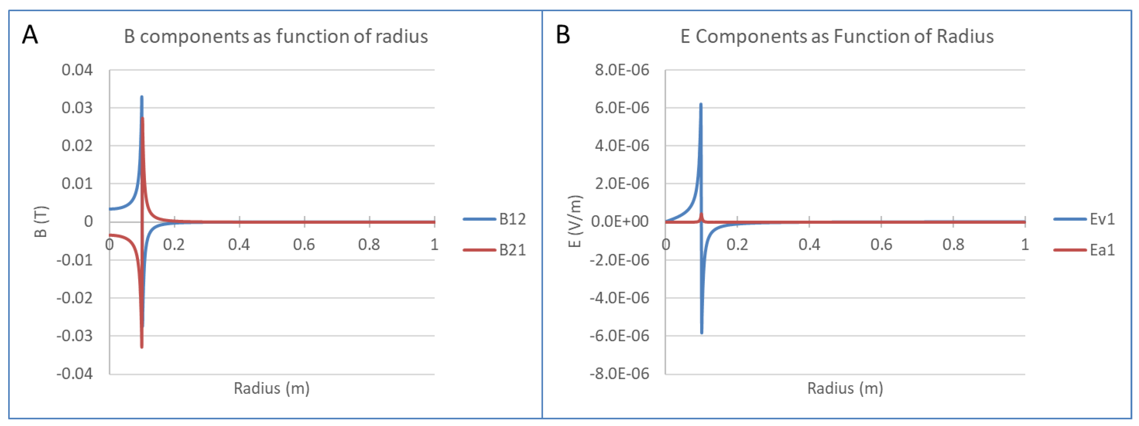
Here, we consider a scenario in which the solenoid is short and the current is constant. The solenoid length is reduced to 0.01 m, and all other parameters are the same as those in Section 3. The calculated and components are plotted in Figure 4.
The components are no longer uniform inside the solenoid. Outside the solenoid, the components reverse polarity and gradually decrease with radius (Figure 4a). This behavior is consistent with classical electromagnetism. However, classical electromagnetism predicts a zero electric field both inside and outside the solenoid. In contrast, the field theory of Weber’s electrodynamics predicts non-zero components. Compared with the long solenoid case, the components are dominated by the velocity-related component . The acceleration-related component is relatively small (Figure 4b), and the two components do not cancel each other outside the solenoid.
6. Discussion
In classical electromagnetism, a time-varying electric field generates a magnetic field, and a time-varying magnetic field generates an electric field. The electric and magnetic potentials are typically not regarded as physical quantities, but rather as mathematical tools for calculating electric and magnetic fields. Furthermore, under the principle of locality, field generation must occur locally.
However, in the case of a long solenoid with a slowly varying current, this conventional understanding faces challenges. The magnetic field outside the solenoid is essentially zero, while the magnetic vector potential remains non-zero. To explain the induced tangential electric field outside the solenoid, one must either abandon the principle of locality or assume that the magnetic vector potential is a physical entity. Yet, there is no consensus on which interpretation is correct. Moreover, the explanation based on the magnetic vector potential raises a further question: what generates the magnetic vector potential outside the solenoid? If it is generated by the magnetic field inside the solenoid, this again implies non-locality.
In contrast, the explanation provided by the field theory of Weber’s electrodynamics is simpler and more direct. The solenoid wire contains stationary positive charges and moving electrons (negative charges). The combined effects of these charges produce electric fields, which can have six components. Since the positive and negative charges are balanced, three of these components are zero. The remaining three non-zero components include the component (equivalent to the magnetic field), a velocity-dependent component, and an acceleration-dependent component. Unlike in classical electromagnetism, these components are independent of each other. The electric field is not generated by the magnetic field; rather, all components are generated directly by the motion of electrons in the solenoid.
The electric fields in Weber’s electrodynamics are non-local, similar to the Coulomb field produced by a stationary charge. The apparent contradiction between non-locality ("action at a distance") and the principle of locality can be reconciled, as discussed in detail in a previous paper [15]. Essentially, the electric fields in Weber’s electrodynamics can form waves due to the presence of virtual charges (many-body effects) in a polarizable vacuum [16,17].
In this paper, the current variation is slow (1 Hz), so radiative effects can be neglected. However, when the frequency of current variation is high (>6 kHz), observed electromotive force (emf) deviates from the linear Weber force prediction [13]. Explaining this deviation may require incorporating radiation effects.
For a long solenoid, the velocity-related and acceleration-related electric fields cancel each other outside the solenoid. This may be one reason why previous experiments failed to detect the velocity-related electric field [18]. In the case of a short solenoid, the velocity-related electric field is not canceled by the acceleration-related component. However, this field is quite weak and may be difficult to detect.
7. Conclusions
In this paper, we provided a simple and straightforward explanation of the Maxwell-Lodge effect using the electric field theory of Weber’s electrodynamics. The tangential electric field is generated directly by the moving electrons in the solenoid, rather than being induced by the magnetic field or magnetic vector potential. Additionally, we demonstrated the different components of the electric field both inside and outside long and short solenoids, highlighting their similarities and differences compared to classical electromagnetism.
Acknowledgments
We thank Andre Koch Torres Assis for his constructive feedback.
References
- Oliver Lodge (1889). "On an Electrostatic Field produced by varying Magnetic Induction". The Philosophical Magazine. 27 (1): 469–479.
- G. Rousseaux, R. Kofman, O. Minazzoli (2008). "The Maxwell-Lodge effect: significance of electromagnetic potentials in the classical theory". The European Physical Journal D. 49 (2): 249–256.
- Assis, Andre & Hernandes, Julio. (2007). The Electric Force of a Current: Weber and the Surface Charges of Resistive Conductors Carrying Steady Currents.
- Kühn, Steffen & Gray, Robert. (2019). Proof of the inconsistency of the full set of Maxwell’s equations with the Maxwell-Lodge experiment. [CrossRef]
- Gray, Robert. (2019). Experimental Disproof of Maxwell and Related Theories of Classical Electrodynamics. Available online: https://www.researchgate.net/publication/335777516.
- Kühn, Steffen. (2020). The Exact Solution of the Maxwell Equations for an Infinitely Long Solenoid. [CrossRef]
- J. C. Maxwell (1873). "A treatise on electricity and magnetism". II. Oxford: Clarendon press: 27–28.
- Heras, José & Heras, Ricardo. (2021). Can classical electrodynamics predict nonlocal effects?. The European Physical Journal Plus. 136. [CrossRef]
- Shoji, Y. & Daibo, M.. (2023). Differential behavior of magnetic field and magnetic vector potential in an optically pumped Rb atomic magnetometer. AIP Advances. 13. 025127. [CrossRef]
- Giuliani, Giuseppe. (2023). Electromagnetic induction: How the “flux rule” has superseded Maxwell’s general law. American Journal of Physics. 91. 278-287. [CrossRef]
- Reed, Donald & Hively, Lee. (2020). Implications of Gauge-Free Extended Electrodynamics. Symmetry. 12. 2110. [CrossRef]
- Vladimir, Leus & T., Smith & Maher, Simon. (2013). The Physical Entity of Vector Potential in Electromagnetism. Applied Physics Research. 5. 56-56. [CrossRef]
- Smith, Ray & Taylor, S. & Maher, Simon. (2014). Modelling electromagnetic induction via accelerated electron motion. Canadian Journal of Physics. 93. 802-806. [CrossRef]
- Li, Qingsong (2021) Electric Field Theory Based on Weber’s Electrodynamics. Int J Magnetics Electromagnetism 7:039.
- Li, Q., Smith, R. T., & Maher, S. (2024). Instantaneous action at a distance and the principle of locality: A new proposal about their possible connection. Preprints, 2024041741.
- Li, Q., & Maher, S. (2023). Deriving an electric wave equation from Weber’s electrodynamics. Foundations, 3(2), 323-334.
- Li, Q. (2025). Transverse wave equation from Weber’s electrodynamics. Preprints, 2025020649.
- D.K. Lemon, W.F. Edwards, C.S. Kenyon, Electric potentials associated with steady currents in superconducting coils. Physics Letters A. 162 (2): 105–114. 1992.
Figure 1.
A) Schematic diagram of the solenoid; B) Top-down view of the solenoid with radius ; C) Side view of the solenoid, showing the electrical action at point A (located at ,,) due to a current segment .
Figure 1.
A) Schematic diagram of the solenoid; B) Top-down view of the solenoid with radius ; C) Side view of the solenoid, showing the electrical action at point A (located at ,,) due to a current segment .
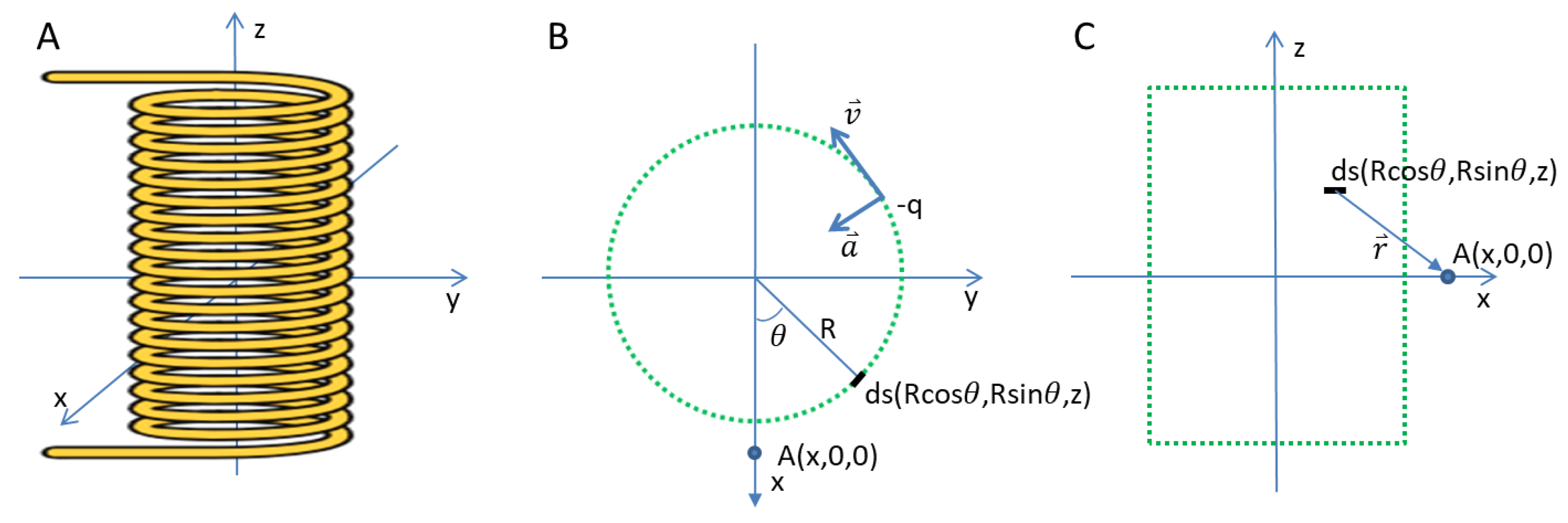
Figure 2.
A) components (, ) and the magnetic field from classical electromagnetism as a function of radius; B) components (Ev1), (Ea1), and their summation (Ev1 + Ea1) as a function of radius.
Figure 2.
A) components (, ) and the magnetic field from classical electromagnetism as a function of radius; B) components (Ev1), (Ea1), and their summation (Ev1 + Ea1) as a function of radius.
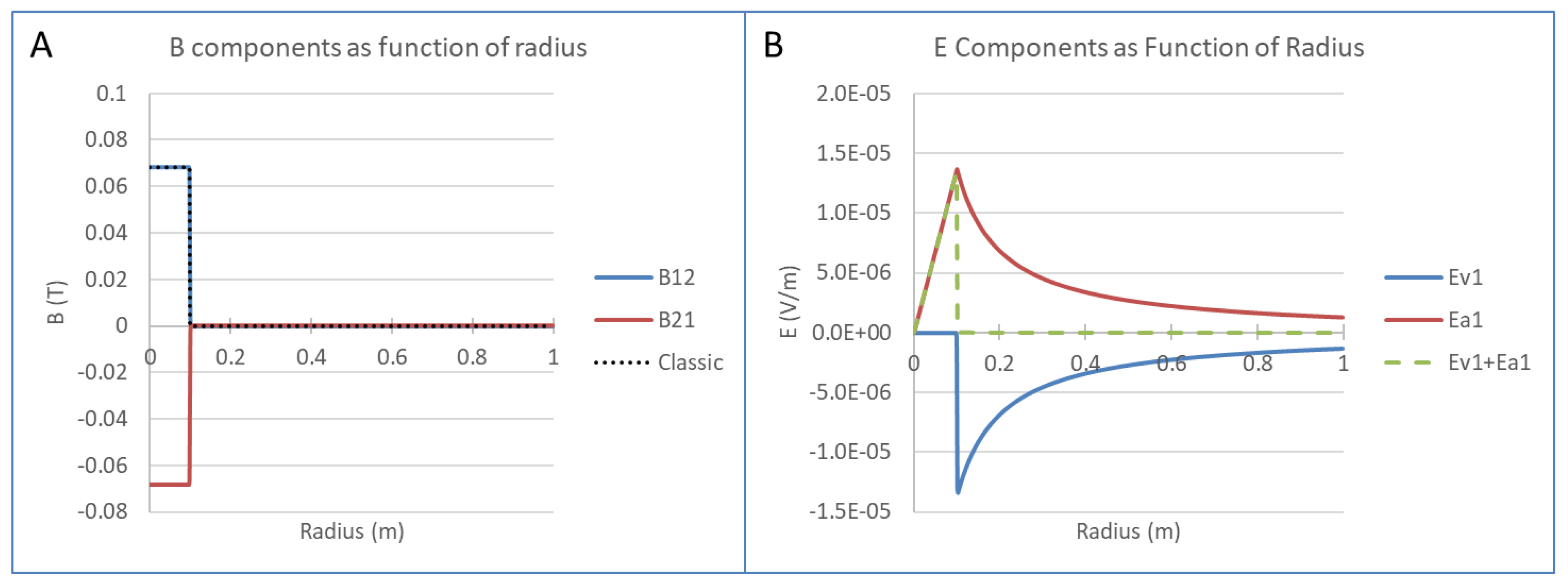
Figure 3.
A) Top-down view of the solenoid with radius ; B) component (Ea2) and the electric field from classical electromagnetism as a function of radius.
Figure 3.
A) Top-down view of the solenoid with radius ; B) component (Ea2) and the electric field from classical electromagnetism as a function of radius.
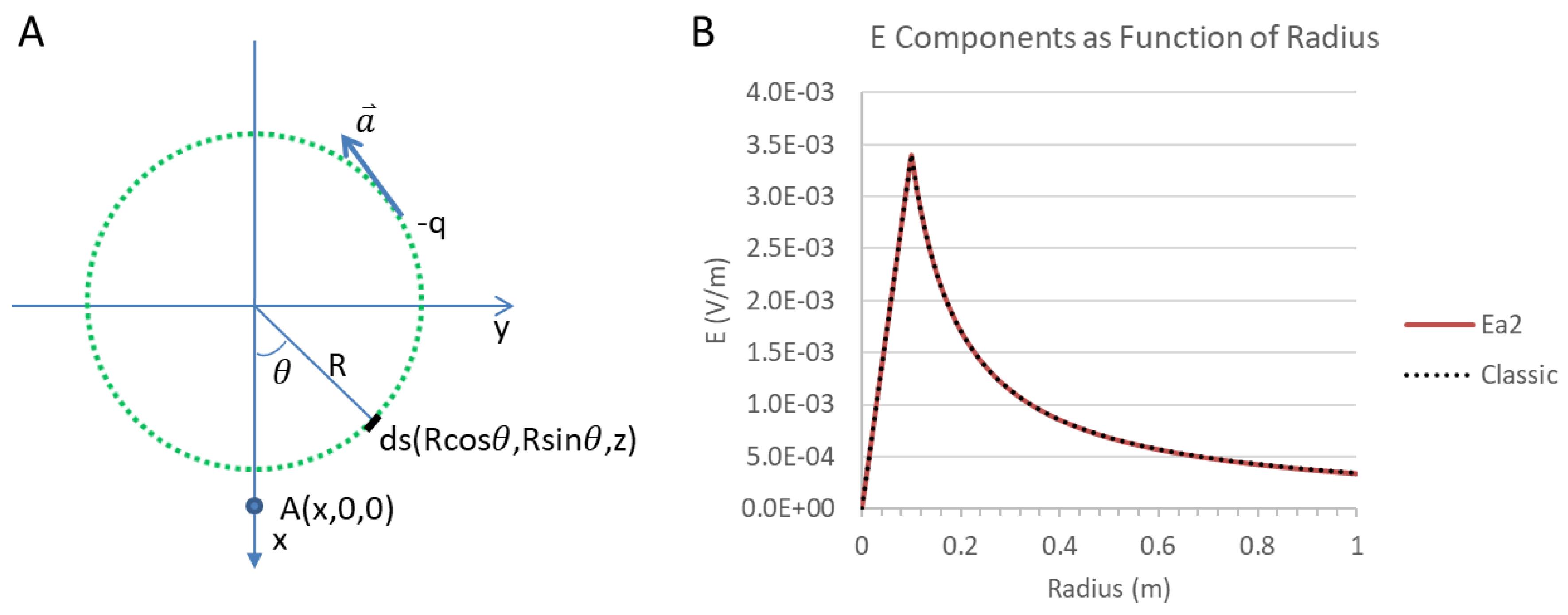
Figure 4.
A) components (, ) as a function of radius; B) components (Ev1), (Ea1) as a function of radius.
Figure 4.
A) components (, ) as a function of radius; B) components (Ev1), (Ea1) as a function of radius.
Disclaimer/Publisher’s Note: The statements, opinions and data contained in all publications are solely those of the individual author(s) and contributor(s) and not of MDPI and/or the editor(s). MDPI and/or the editor(s) disclaim responsibility for any injury to people or property resulting from any ideas, methods, instructions or products referred to in the content. |
© 2025 by the authors. Licensee MDPI, Basel, Switzerland. This article is an open access article distributed under the terms and conditions of the Creative Commons Attribution (CC BY) license (http://creativecommons.org/licenses/by/4.0/).
Copyright: This open access article is published under a Creative Commons CC BY 4.0 license, which permit the free download, distribution, and reuse, provided that the author and preprint are cited in any reuse.


