
Submitted:
21 April 2025
Posted:
22 April 2025
You are already at the latest version
Abstract
Urban vulnerability creates structural imbalances, leading to unsafe conditions and urban decline. One of the key root causes of urban vulnerability is significant changes in urban morphology. This study aims to examine the morphological structural factors that influenced physical vulnerability, with a focus on commercial buildings, which were affected by morphological structures at the global, local, and community levels, depending on their location; these factors contributed to spatial vulnerability in varying degrees.This study applied the indicator-based quantitative research methodology, constructing a Physical Vulnerability Index (PVI) by using Principal Component Analysis (PCA) to create new factors or components and compare physical vulnerability levels across different areas. The research findings found that the most influential morphological structural factor on physical vulnerability was micro-level morphology, primarily due to the relationship between the configuration of space and the level of usage popularity. The second most influential factor is macro-level morphology, resulting from the relationship between the accessibility potential of urban-level and neighborhood-level transportation networks.
Keywords:
urban morphology
; urban vulnerability
; physical vulnerability
; space syntax theory
; Principal Component Analysis (PCA)
1. Introduction
Urban vulnerability is considered a dynamic pressure stemming from root causes of susceptibility within the urban system, encompassing physical, economic, and social aspects. It affects the exposure to and accumulation of negative externalities, creating structural imbalances that lead to unsafe conditions in cities [1,2,3,4,5,6,7].
Urban vulnerability varies depending on spatial context [2,3,8], so-called “place-based approaches” [9]. One of the key root causes of urban vulnerability is significant transformations in urban morphology, which lead to urban decline. This can be observed through completely empty streets, abandoned buildings, and underutilized infrastructure, resulting in the slow degradation of urban spatial configuration. This gradual deterioration diminishes the vibrancy of the city and contributes to the loss of its central role in attracting visitors and economic activities [10].
Currently, space syntax theory—an important theoretical approach focused on studying the characteristics of urban morphology to maintain the centrality of cities—supports the principle that urban morphology, derived from the street network, influences the potential for accessibility. This theory can be used to predict the popularity of public space usage, patterns of pedestrian and vehicular movement, and the distribution of land use and density based on movement patterns, in order to assess the growth and decline of cities both in the present and future [11,12,13,14,15,16,17,18].
Therefore, studying the characteristics of urban morphology can help identify the root causes or factors influencing urban vulnerability. However, there is still a lack of research that can empirically and systematically explain the morphological factors at the global, local, and community levels that influence physical vulnerability in urban areas. This gap in the research is the basis for the study's objective: to examine the morphological factors that influence physical vulnerability, while the research question is: “Which morphological factor has the greatest influence on physical vulnerability?”
In this study, the focus is on commercial buildings, which are influenced by morphological structures at different spatial levels—global, local, and community—that, in turn, affect spatial vulnerability according to space syntax theory. The research methodology applies a quantitative, indicator-based approach by developing a Physical Vulnerability Index (PVI) to enable comparisons of physical vulnerability levels between different areas or units of analysis based on varying morphological characteristics. The findings of this study can lead to the identification of root causes and a deeper understanding of the morphological factors in urban areas that cause spatial vulnerability and unsafe urban environments.
2. Research Area
Given that the characteristics of vulnerability vary according to spatial context or the unit of analysis [2,9], this study defines the unit of analysis as a group of 60 commercial building areas connected to the main road‒Pattanakarn Kukwang Road‒which is considered the central area of Nakhon Si Thammarat City in southern Thailand. The city center and main roads, identified through space syntax analysis, are represented by red axial lines. These lines were computed high global integration and local integration values, as shown in Figure 1.
Each group of commercial buildings is influenced by the morphological structure of the transportation network at different levels. Therefore, the selected study area and unit of analysis can theoretically represent and be used to analyze the morphological factors influencing physical vulnerability.
3. Literature Review
This indicator-based quantitative study defines research variables by developing a Physical Vulnerability Index (PVI) based on literature review. Grounded on the literature review, the following morphological characteristics that influence physical vulnerability are identified:
3.1. Urban Street Networks
According to the space syntax theory, the morphological structure of urban street networks determines accessibility potential at both the global and local levels, affecting human behavior in spatial organization and resulting in different spatial characteristics [11,12,17]. A densely interconnected street network at the global level, with a grid system and small street blocks, offers a morphological structure that enhances accessibility, offers diverse travel options, supports economic activities, and creates a vibrant urban environment with high pedestrian activity, contributing to a “live center” [11,15]. Additionally, local street networks that effectively integrate into the city-wide transportation system can benefit from “natural movements” on account of the city’s vitality [11,17,19].
3.2. Public Space Connectivity Patterns
Hillier and Hanson (1984), proposed that the structure of street networks within communities directly affects connectivity and the arrangement of public spaces within cities, as well as changes in building density, land use, and building utilization. Street network structures can be categorized into two types as follows [12]:
1) Beady ring structure: A distributed system where public spaces are well-connected to main roads, facilitating convenient city travel. This includes grid and ring/loop street patterns.
2) Tree-like structure: A non-distributed system where public spaces are not well-connected, with most roads leading to dead ends or cul-de-sacs. Movement within the city with this pattern requires returning to the main road each time [20].
New Urbanism Theory supports permeable grid street layouts over cul-de-sac designs. Cul-de-sac layouts, which prioritize car traffic, are less friendly to pedestrians and can encourage crime, whereas grid layouts rely less on cars, promote walkability, and reduce crime [21], enhancing natural surveillance and “eyes on the street” [22].
3.3. Transportation Networks Sustained by Natural Movement of People and Economic Activities
Jacob (1961) stated that streets and sidewalks sustained by the passage of people are indicators of urban quality, creating “eyes on the street” that foster social interaction and the vitality of the city [12,17,23]. This aligns with Jan Gehl’s (2011) concept, which asserts that streets and public spaces must accommodate people and activities at various times, including social and alternative activities, to make the city meaningful and attractive [24].
Furthermore, increasing “eyes on the street” enhances urban safety through the natural surveillance provided by passing pedestrians. This has a positive impact on perceptions of safety and effectively reduces crime [25]. This is consistent with Oscar Newman’s “defensible space” concept, which suggests that designing buildings and communities to support diversity of use and highly used pedestrian streets fosters natural surveillance by residents, which is crucial for crime prevention [26]. The Crime Prevention Through Environmental Design (CPTED) approach also emphasizes designing environments that promote natural surveillance to influence human behavior, reduce fear, and lower the likelihood of crime [27,28].
3.4. Visibility
A transportation network or public space with high visibility or a wide isovist field facilitates pedestrian activity among various groups of people [29,30]. Thus, visibility is an important dimension that determines accessibility and route choice [31].
Moreover, visibility is a key factor behind surveillance, affecting perceptions of safety by increasing the number of “eyes on the street”[32], which is a significant factor affecting fear of crime in the environmental contexts [33,34]. Buildings located deep from main streets or behind gated communities affect perceptions of safety due to lower visibility, resulting in fewer passersby [35].
Areas with dense building utilization, where buildings have numerous doors opening directly onto the street, are known as active frontages. This mechanism creates “eyes on the street” [23] and motivates walking, and the use of public spaces [24]. It also enhances the visibility of buildings to the street, referred to as “street intervisibility,” which influences social control and the degree of liveliness on the street [36].
Based on the literature review, a total of 9 urban morphology variables influencing physical vulnerability are identified in Table 1.
4. Research Methodology
The development of the Physical Vulnerability Index (PVI) involved quantitative research based on an indicator-based approach to enable comparison between areas or analytical units. This approach was adapted from Cutter’s et al. (2003), Social Vulnerability Index (SoVI) [7,37], as demonstrated in the following steps:
4.1. Data Preparation for Developing the Physical Vulnerability Index (PVI)
4.1.1. Preliminary Agreement Analysis
To conduct Principal Component Analysis (PCA) through factor analysis, the data must meet the following preliminary conditions. First, the number of units of analysis should exceed 30 units. Second, the number of variables used to create the Physical Vulnerability Index should have a ratio of at least 3 units of analysis per 1 variable.
In this study, the units of analysis were 60 commercial building locations (more than 30 units), with a total of 9 variables, resulting in a ratio of 6.6 units of analysis per variable, which is deemed suitable for performing Principal Component Analysis (PCA).
4.1.2. Data Collection Methods for Each Variable
The data selected for the component analysis must consist of continuous variables or those on an interval scale and ratio scale to construct the Physical Vulnerability Index, are presented in Table 2.
According to the table, the data collection methods for variables affecting physical vulnerability include:
4.1.2.1. Space Syntax Methods
Urban morphology analysis known as “space syntax methods” is a physical model, in the form of a set of mathematical formulas, that can be empirically measured [12,38,39]. It allows for the analysis of the level of accessibility of urban street networks through the “Depthmap” program [40].
The analysis of urban street networks using space syntax methods demonstrates the following values:
1) Integration value
The Integration Value refers to the degree of spatial aggregation or dispersion between any given space and other spaces. The higher the value, the greater the accessibility potential. Integration value is divided into two levels:
- Global integration value (Rn, n-step): This measures the connectivity of the selected street with all other streets in the system, known as the integration values of axial lines at an infinite radius or “radius n.” This represents the overall relationship, showing the main streets at the global level [13].
- Local integration value (R3, 3 steps): This measures the connectivity of the selected street with the two adjacent connected streets and extends only to the next street in the sequence, without considering the entire system. This is referred to as “radius 3” and shows specific local relationships. Thus, this measurement indicates which streets are most commonly used at the neighborhood level [13].
2) Mean depth (MD)
Mean Depth (MD) can be calculated by creating a justified graph or J-graph, which allows for urban morphology analysis, such as dead-end streets and grid/loop streets. This can predict movement behavior and influence land use and building patterns [13].
Mean Depth is determined by assigning a depth value to each space based on its distance from the original space. The total of these depth values is then summed and divided by the number of spaces in the system minus one (excluding the original space) [12,41,42]. The formula used for calculation is:
where k = the number of spaces in the system.
Mean Depth (MD) = sum total depth (TD) / (k - 1)
A lower Mean Depth (MD) indicates easier accessibility, with higher pedestrian flow, while a higher Mean Depth (MD) indicates more difficult accessibility and lower pedestrian flow [13].
3) Relative Asymmetry (RA)
Relative asymmetry assesses the depth of a system from a specific point by comparing it to its theoretical maximum and minimum depths. The minimum depth occurs when all spaces are directly connected to the original point, while the maximum depth is reached when the spaces are arranged in a linear sequence, with each additional space adding an extra level of depth. This comparison provides a theoretical normalization of the total depth [12,42]. The formula used for calculation is:
where MD = Mean Depth and k = the number of spaces in the system.
Relative Asymmetry (RA) = 2 (MD - 1) / (k - 2)
The calculated value indicates that if RA approaches 1, the transportation network is a non-distributed system with a linear pattern, such as a dead-end or cul-de-sac street system. Conversely, if RA approaches 0, the transportation network is a distributed system with a bush-like pattern, such as a grid street system [12,42].
4.1.2.2. Degree of Street Intervisibility
The method for analyzing the degree of street intervisibility, adapted from previous studies [36,43,44,45], involves the following steps:
(1) The registration of the number of building entrances and adjacent windows facing public areas shows how building entrances connect directly to streets and public spaces in the city. The interaction between the building façade and the sidewalk and street (building-street interfaces) can be classified into three types as follows:
Type 1: 71-100% Building façades with doors and windows facing the street directly, where the ground floor is visible and accessible to people, are considered active frontages and are given a value of 1.
Type 2: 31-70% Building façades with doors and windows facing the street directly, where the ground floor is semi visible to people, are considered semi-active frontages and are given a value of 0.5.
Type 3: 0-30% Building façades with doors and windows facing the street directly, with no direct interaction with the street, where people cannot see activities inside the building due to closed doors or windows, are considered non-active frontages and are given a value of 0
(2) The Measurement of the degrees of street intervisibility for each location involves the following variables:
where AF = the total active frontages value of each building in the street segment. NB = the total number of buildings in the street segment
Degrees of street intervisibility = AF/NB
4.1.2.3. Gate Count
The gate count method involves surveying by photographing, measuring, recording, and setting up counting points to determine the level of natural movement based on the movement ratio. This is calculated by counting the number of vehicles and people passing through the street network during a specified time period.
In this study, a total of 60 counting points were established at locations along the commercial building areas connected to main streets. Counting and recording of vehicle movements were conducted on weekdays (Monday, Wednesday, Friday) and weekends (Saturday). Each day was divided into four time-intervals for data collection: Interval 1 (8:00‒11:00), Interval 2 (11:00‒14:00), Interval 3 (14:00‒17:00), and Interval 4 (17:00‒20:00). During each interval, vehicle counts were recorded every 10 minutes at each counting point.
4.2. Principal Component Analysis (PCA)
Principal Component Analysis (PCA), a method of factor analysis, involves the following steps:
4.2.1. Variable Standardization
Standardize all variables using Z-score normalization, which converts the data to a common scale with a mean of 0 and a standard deviation of 1.
4.2.2. Correlation Matrix
Determine the relationships between all variables using a correlation matrix. This matrix contains the correlation coefficients of the variables, which should be greater than 0.3. Additionally, the Kaiser-Meyer-Olkin (KMO) measure is used to assess the suitability of the data for factor analysis. The KMO value ranges from 0 to 1, with a value greater than 0.6 indicating adequate sampling for PCA.
4.2.3. Factor Extraction
Extract factors using PCA to reduce data complexity by identifying the smallest number of factors that can explain the majority of the variance in the data. This involves calculating communalities for each indicator. Variables with high communalities (greater than 0.5) are considered suitable for inclusion in the extracted factors.
4.2.4. Factor Rotation
Rotate the factors using orthogonal rotation techniques, such as Varimax, to enhance interpretability. This process adjusts the factor loadings and the percentage of variance explained by each new factor. After rotation, variables are grouped based on their factor loadings, with a focus on those with loadings between 0.5 and 1, or -0.5 and -1.
4.2.5. Interpretation and Factor Analysis
Analyze the results of PCA to group related variables into new factors, which can be named based on their influence on physical vulnerability. Factors are interpreted and ranked according to their variance contribution, creating a new factor called “structural factors influencing physical vulnerability.”
4.3. Physical Vulnerability Index (PVI)
The Physical Vulnerability Index (PVI) is calculated by aggregating the scores of selected components to compare vulnerability levels between units of analysis—in this case, commercial buildings in various locations. The calculation is based on the following formula [46]:
PVI j = 
Physical Vulnerability Index (PVI) = physical vulnerability value
Variance = proportion of variance explained by the indicator group (expressed as a percentage)
Factor loading = weight or correlation of the component with the indicator
Z-Score = score of the factor used in the calculation
i = sequence of the indicator group derived from the analysis
j = sequence of the study area
n = sequence of the final number
The Physical Vulnerability Index PVI) calculated will be standardized by transforming the component scores into a common scale, with a mean of 0 and a standard deviation of 1. This transformation results in a standardized value equivalent to the original variables, and the final result is referred to as the “Physical Vulnerability Score.”
5. Research Results
5.1. Descriptive Statistics
Based on the data preparation for developing the Physical Vulnerability Index (PVI), the descriptive statistics of 9 variables from the data of 60 spatial units are illustrated in Table 3.
5.2. Principal Component Analysis (PCA)
The development of indicators involved standardizing all data using Z-score normalization, leading to the development of the Physical Vulnerability Index through Principal Component Analysis (PCA) in factor analysis. The results are presented as follows:
5.2.1. Correlation matrix
1) The results of the KMO and Bartlett's Test for reliability analysis and checking the suitability of the dataset for Principal Component Analysis (PCA) [47], are presented in Table 4.
As shown in the KMO and Bartlett's Test Results table, the analysis of the correlation matrix showed that the KMO (Kaiser-Meyer-Olkin) value was 0.817, which was greater than 0.6. This indicates that the variables were suitable for component analysis, and a value greater than 0.8 suggested the dataset was highly appropriate for component analysis.
2) When examining the variance of each variable, considering the anti-image correlation values displayed along the diagonal of the anti-image matrices, it was found that all variables had values greater than 0.5, indicating suitability for component analysis.
3) Checking the communalities from the factor extraction revealed that the communalities of each variable were greater than 0.5 and close to 1, making them suitable for grouping into components.
5.2.2. Factor extraction
The Rotated Component Matrix showed that all 9 variables could be reorganized into two different componential categories, are presented in Table 5. This categorization was based on the variables in the vertical rows that had a factor loading greater than 0.5 and close to 1. The factor loadings of each variable were used in the next step to calculate the Physical Vulnerability Index (PVI).
5.2.3. Factor rotation
The Total Variance Explained table can be interpreted as follows:
1) The Component column indicates that 2 components were extracted from the 9 variables related to physical vulnerability.
2) The Rotation sums of squared loadings column refers to the eigenvalues of each variable after component extraction and orthogonal rotation using the Varimax method. Only variables with an initial eigenvalue greater than 1 were considered. The components consisted of:
- Component 1 included 7 variables: Vacancy Rate, Degree of Street Intervisibility, Utilization Rate of Commercial Buildings, Mean Depth (MD), Degree of Natural Movement, Connectivity of the location to the main road, and Visibility potential from the street to the building. These variables, ordered by their factor loading (from most to least influential), explain 55.399% of the total variance.
- Component 2 included 2 variables: Global Integration and Local Integration. These variables, also ordered by their factor loading, account for 26.184% of the total variance.
Therefore, according to the rotated component matrix and the Total Variance Explained table, the variables could be grouped into 2 new components. For each new component, the factor loadings of the variables and the percentage of variance explained by the component are summarized in Table 6.
Table 7 shows the characteristics of variables that exhibited positive or negative correlations, which were used for calculating the Physical Vulnerability Index (PVI), as explained below:
Component 1 was divided into two subgroups: negative variables and positive variables.
- The negative variables subgroup included three variables: building vacancy rate, connectivity of the location to the main road, and depth of the location relative to the main road. This means that as the values of the negative variables increase, the level of physical vulnerability also increases.
- The positive variables subgroup included four variables: degree of street intervisibility, utilization rate of commercial buildings, degree of natural movement, and visibility from the road to the building. This means that as the values of the positive variables increase, the level of physical vulnerability decreases.
The relationship between these two subgroups indicated an inverse relationship: as the values of the negative variables increased, the values of the positive variables decreased.
On the other hand, Component 2 consisted of two positive variables that correlated in the same direction, meaning that as the values of these positive variables increased, the level of physical vulnerability decreased.
5.2.4. Component analysis and interpretation
Based on the Principal Component Analysis (PCA) of the factor analysis, variables with similar relationships were grouped together to form new factors termed “factors affecting physical vulnerability.” These factors can be interpreted and ranked in order of importance based on the variance of the variable sets within them.
First, Component 1 Micro-level Morphological Structure, this refers to the relationship between the “configuration of space” and the “characteristics and popularity of space usage.” The configuration of space refers to the physical attributes, including shapes, forms, and spaces of the project's location, the connectivity of the location to the main road, and the depth of the location relative to the main road. Additionally, the characteristics and popularity of space usage refer to the activities that occur both inside and outside the project, which include building utilization, the degree of natural movement of people, and visibility that shows the interaction between people, streets, and buildings. Therefore, the relationship between the configuration of space and the characteristics and popularity of space usage turns the space of the location into vibrant places.
Second, Component 2 Macro-level Morphological Structure, this refers to the relationship between the location and the urban street networks at the global and local levels, which influence the accessibility potential at both levels. This impacts the attraction of natural movement of people, economic activities, and land use according to the principles of the movement economy. Thus, the location of a project influenced by the morphological structure of the global and local street networks will benefit from a higher level of natural movement. As a result, commercial buildings are more likely to benefit from increased opportunities for passing traffic.
5.3. Physical Vulnerability Index (PVI) Development
The development of the Physical Vulnerability Index (PVI) involved combining selected component scores and ranking the physical vulnerability index to enable comparisons between the units of commercial buildings. The data was then standardized using Z-score normalization, setting the mean to 0 and the standard deviation to 1. This standardization process allowed the components to be transformed into a linear combination similar to the original variables.
The resulting value, known as the “Physical Vulnerability Score (PVScore),” was used to categorize the Physical Vulnerability Index (PVI) into four levels: low, moderately low, moderately high, and high.
The analysis results of the Physical Vulnerability Index (PVI) for 60 commercial building areas revealed that 11 areas had a low level of physical vulnerability, 15 areas had a slightly below-average level, 26 areas had a slightly above-average level, and 8 areas had a high level of physical vulnerability. The results are illustrated in the descriptive statistics in Table 8, Table 9, Table 10 and Table 11, and the physical characteristics of the commercial building areas according to their level of physical vulnerability are presented in Figure 3, Figure 4, Figure 5 and Figure 6. Additionally, the analysis results were used to create a map positioning the commercial building areas, known as the “Physical Vulnerability Index (PVI) Map,” which allowed for the comparison of physical vulnerability levels between areas and showed the distribution of physical vulnerability varying according to the characteristics of urban morphology, as depicted in Figure 2.
6. Discussion
The results from the analysis of the Physical Vulnerability Index (PVI) led to the development of two new components: Component 1 Micro-level Morphological Structure and Component 2 Macro-level Morphological Structure.
The study results showed that Component 1 (micro-level morphological structure) had 2.11 times more influence on physical vulnerability compared to Component 2 (macro-level morphological structure). This conclusion was based on the percentage of variance (% of Variance) of the new component groups, as illustrated in Table 12 below.
The components and factors related to the spatial morphology affecting physical vulnerability are summarized below:
First, the concept of “Component 1 Micro-level Spatial Structure” align with the study by Hillier and Hanson (1984), which indicates that the structural characteristics of the internal circulation within communities directly impact the connectivity network and the arrangement of public space within cities, influencing land use and buildings in surrounding areas [12]. It is also consistent with Nes & López (2007), who noted that the micro-scale spatial level affects the vibrancy of urban areas [41]. This research shows that Component 1, the micro-scale spatial structure, resulting from the relationship between the configuration of space and the characteristics and levels of space usage, had a higher influence on physical vulnerability than macro-scale spatial structures. This component consisted of two major factors as follows:
6.1. Configuration of Space
According to the Physical Vulnerability Index (PVI), it was found that the areas or locations of commercial buildings with the highest levels of vulnerability consisted of 8 units with the following common spatial characteristics.
6.1.1. The connectivity of the location to main roads was low
This is demonstrated by 4 out of the 8 units having a Relative Asymmetry (RA) value of 1, indicating that these 4 units had road networks characterized as non-distributed systems, such as dead-end streets or cul-de-sacs.
6.1.2. The depth between the location and main roads was high
This is evidenced by 4 out of the 8 units having an average Mean Depth (MD) value of 2.125, compared to the overall average Mean Depth (MD) value of 1.3148. This shows that these 4 units were located deeper and were harder to access, resulting in fewer opportunities for pedestrian traffic, even though the road networks may be distributed systems, such as grid or ring/loop patterns.
6.1.3. The visibility from the street to the building was low
This is shown by the 8 high-vulnerability units having an average Street Width of 6.25 meters, compared to an average Street Width of 10.77 meters for all units. This indicates that these 8 units had relatively narrow isovist fields, affecting accessibility and route choice.
6.2. Characteristics and Levels of Usage
The characteristics and levels of usage of the areas, as shown by the 8 units with the highest levels of vulnerability, can be summarized as follows:
6.2.1. The rate of building vacancy was high
This is demonstrated by the 8 high-vulnerability units having an average vacancy rate of 73.71%, while the average vacancy rate for all units was 32.41%. This indicates that the 8 units had a significant number of vacant and abandoned buildings.
6.2.2. The visibility of buildings from the street was low
This is evidenced by the 8 high-vulnerability units having an average degree of street intervisibility of 0.16, compared to an average degree of street intervisibility of 0.61 for all units. This suggests that the 8 units had a high proportion of non-active frontages, lacking interaction between buildings and streets.
6.2.3. The utilization rate of commercial buildings was low
This is shown by the 8 high-vulnerability units having an average commercial building utilization rate of 12.04%, while the average rate for all units was 56.16%. This indicates that the 8 units had low utilization rates, consistent with the intended purpose of the buildings.
6.2.4. The level of natural movement was low
This is illustrated by the 8 high-vulnerability units having an average vehicle movement ratio of 5.48 vehicles per hour, while the average vehicle movement ratio for all units was 50.63 vehicles per hour. This indicates that the 8 units had a low capacity to attract pedestrian traffic.
Second, Component 2 Macro-level Morphology is considered a secondary factor influencing physical vulnerability. It reflects the relationship between urban and neighborhood street networks. This aligns with space syntax theory, which states that the structure of urban street networks determines accessibility at both global and local levels, affecting pedestrian movement and attracting economic activity, thereby creating “live centers” [11,15]. In contrast, street networks with low accessibility at both urban and neighborhood levels are not sustained by natural movement over time. This creates negative attractors and reduces pedestrian traffic [17], leading to lacunas in the natural movement system and urban decay, respectively [19].
This study shows that Component 2 resulted from the relationship between urban and neighborhood street networks, contributing to physical vulnerability. The 8 units with the highest physical vulnerability shared the following characteristics of macro-scale morphology:
1) The urban accessibility potential was low. Among the 8 high-vulnerability units, 3 units had Global Integration values lower than 0.7197, the average for all units. These units were located deep from main roads, resulting in low accessibility and insufficient natural movement.
The remaining 5 units had Global Integration values higher than the average, indicating high accessibility potential. However, these 5 units still had high physical vulnerability due to the influence of micro-scale morphology, which had a greater effect on physical vulnerability than macro-scale morphology. Component 1 accounted for 55.399% of the variance, whereas Component 2 made up 26.184% of the variance, which was 2.116 times less.
2) The neighborhood accessibility potential was low. Among the 8 high-vulnerability units, 6 had Local Integration values lower than 1.9640, the average for all units. This indicates low accessibility potential in the neighborhood street network.
The remaining 2 units, although having Local Integration values higher than the average, were in dead-end street networks, as indicated by a Relative Asymmetry (RA) value of 1. This affected the integration of neighborhood street networks into the urban network, a crucial factor in determining neighborhood accessibility potential.
7. Conclusions
The analysis of the Physical Vulnerability Index (PVI) revealed that the variables identified from the literature review could be grouped into two new components influencing physical vulnerability. On one hand, Component 1 Micro-level Morphology was identified as the most significant factor affecting physical vulnerability. This component results from the relationship between the configuration of space and the level of land use. On the other hand, Component 2 Macro-level Morphology was the secondary factor, derived from the relationship between the accessibility potential of urban and neighborhood street networks.
Additionally, within the first component, there were three specific spatial characteristics significantly affecting physical vulnerability. First, the spatial morphology exhibited a non-distributed system pattern, such as dead ends or cul-de-sacs. This pattern indicated street networks that did not connect to other networks, limiting accessibility. Second, the depth of the location from the main road was high, making access difficult and causing fewer opportunities for pedestrian traffic. Third, low visibility from the street to buildings resulted in narrow isovist fields, which affected accessibility and route selection. These three spatial characteristics were associated with the level of activity and land use rate. They led to vacant buildings, underutilized spaces, reduced pedestrian traffic, and diminished interaction between buildings and streets.
The second component showed that the influence of global urban street networks was a crucial factor in determining accessibility. Buildings directly connected to main roads benefited from natural movement and attracted high economic activity, resulting in lower physical vulnerability. Additionally, commercial buildings that were not directly connected to main roads but had strong connections to local street networks could also benefit from natural movement due to their integration into the global urban network. Therefore, macro-scale morphology resulted from the interaction between global and local street networks, which mutually influenced each other and are significant in determining spatial physical vulnerability.
This study of morphological factors affecting physical vulnerability in commercial buildings demonstrates a systematic quantitative measurement at the local scale. This research fills knowledge gaps in urban morphology theory and highlights the importance of both micro- and macro-scale urban structures, providing a more detailed spatial explanation of urban morphology's impact on physical vulnerability.
The findings underscore the importance of micro-scale morphology, which is often overlooked by urban planners who tend to focus on macro-scale spatial analysis. Development of micro-scale morphology is typically seen as the responsibility of real estate developers. Thus, this study indicates that urban planners and real estate developers need to collaborate to integrate both micro- and macro-scale spatial structures to mitigate negative externalities and reduce urban vulnerability.
Author Contributions
Conceptualization, R.T.; Methodology, R.T.; Software, R.T.; Validation, R.T. and B.C.; Formal analysis, R.T.; Investigation, R.T.; Resources, R.T. and B.C.; Data curation, R.T. and B.C.; Writing—original draft preparation, R.T. and B.C.; Writing—review and editing, R.T. and B.C.; Visualization, R.T. and I.T.; Supervision, R.T.; Project administration, R.T.; Funding acquisition, R.T. and B.C.
Funding
This research was funded by Center of Excellence in Logistics and Business Analytics, School of Management, Walailak University, Nakhon Si Thammarat, Thailand.
Institutional Review Board Statement
Not applicable.
Informed Consent Statement
Not applicable.
Conflicts of Interest
The authors declare no conflicts of interest.
References
- Blaikie, P., Cannon, T., Davis, I., Wisner, B. At risk: natural hazards, people's vulnerability and disasters. Psychology Press, 2004.
- Birkmann, J.; Birkmann, J. Measuring vulnerability to natural hazards: Towards disaster resilient societies. United Nations University Press, 2006.
- Cutter, S.L. Vulnerability to environmental hazards. Prog. Hum. Geog. 1996, 20(4), 529−539. [CrossRef]
- Adger, W.N. Vulnerability. Global Environ. Change 2006, 16(3), 268−281. [CrossRef]
- Fekete, A. Validation of a social vulnerability index in context to river-floods in Germany. Nat. Hazard. Earth Sys. Sci. 2009, 9(2), 393−403. [CrossRef]
- Wisner, B.; Blaikie, P.; Cannon, T.; Davis, I. At risk: Natural hazards, people's vulnerability and disasters. Routledge, 2014. [CrossRef]
- Cutter, S.L.; Boruff, B.J.; Shirley, W.L. Social vulnerability to environmental hazards. Soc. Sci. Quart. 2003, 84(2), 242−261. [CrossRef]
- Fekete, A., Brach, K. Assessment of social vulnerability river floods in Germany: United Nations University, Institute for Environment and Human Security (UNU-EHS), 2010.
- Zakour, M.J.; Gillespie, D.F. Community disaster vulnerability (pp. 978−1001). Springer, New York, 2013. [CrossRef]
- Laursen, L.L.H. Shrinking cities or urban transformation. Institut for Arkitekturog Medieteknologi, 2009.
- Hillier, B. Centrality as a process: Accounting for attraction inequalities in deformed grids. Urban Design Int. 1999, 4(3−4), 107−127. [CrossRef]
- Hillier, B.; Hanson, J. The social logic of space. Cambridge: Press Syndicate of the University of Cambridge, 1984. [CrossRef]
- Hillier, B. Space is the machine: A configurational theory of architecture. Space Syntax, 2007.
- Hillier, B.; Sahbaz, O. An evidence based approach to crime and urban design: Or, can we have vitality, sustainability and security all at once (pp. 1−28). Bartlett School of Graduates Studies University College London, 2008.
- Hillier, B. Cities as movement economies. Urban Design Int. 1996, 1(1), 41−60. [CrossRef]
- Hillier, B.; Sahbaz, O. High resolution analysis of crime patterns in urban street networks: An initial statistical sketch from an ongoing study of a London borough. In Proceedings of the 5th International Symposium Space Syntax, Delft, 2005.
- Hillier, B.; Penn, A.; Hanson, J.; Grajewski, T.; Xu, J. Natural movement: Or, configuration and attraction in urban pedestrian movement. Environ. Plann. B 1993; 20(1), 29−66. [CrossRef]
- Turner, A.; Penn, A. Encoding natural movement as an agent-based system: An investigation into human pedestrian behaviour in the built environment. Environ. Plann. B 2002, 29(4), 473−490. [CrossRef]
- Hillier, B. Space is the machine UK. Cambridge University Press, 1996.
- Carmona, M. Public places, urban spaces: The dimensions of urban design. Routledge, 2010.
- Cozens, P.; Hillier, D. The shape of things to come: New urbanism, the grid and the cul-de-sac. Int. Plann. Stud. 2008, 13(1), 51−73. [CrossRef]
- Hillier, W.; Shu, S. Crime and urban layout: The need for evidence (pp. 224−248). In Ballintyne, S.; Pease, K.; McLaren, V. (Eds.). Secure Foundations: Key Issues in Crime Prevention. London: Crime Reduction and Community Safety, Institute of Public Policy Research, 1999.
- Jacobs, J. The Death and Life of Great American Cities. England. Penguin Books, 1961.
- Gehl, J. Life between Buildings: Using Public Space. Island Press, Washington, DC, 2011.
- Ceccato, V.; Nalla, M.K. Crime and fear in public places: Towards safe, inclusive and sustainable cities. Taylor & Francis, 2020. [CrossRef]
- Newman, O. Defensible space. Macmillan, New York, 1972.
- Crowe, T. Crime prevention through environmental design. Butterworth-Heinemann, 2000.
- Cozens, P. Planning, crime and urban sustainability. WIT Trans. Ecol. Environ. 2007, 102, 10. [CrossRef]
- Benedikt, M.L. To take hold of space: Isovists and isovist fields. Environ. Plann. B 1979, 6(1), 47−65. [CrossRef]
- Batty, M. Exploring isovist fields: Space and shape in architectural and urban morphology. Environ. Plann. B 2001, 28(1), 123−150. [CrossRef]
- Pain, R.H. Social geographies of women’s fear of crime. Trans. Ins. Brit. Geogr. 1997, 22, 231−244.
- Turner, A.; Penn, A. Making isovists syntactic: Isovist integration analysis. In Proceedings of the 2nd International Symposium on Space Syntax, Brasilia, 1999.
- Lee, S.; Ha, M. The duality of visibility: Does visibility increase or decrease the fear of crime in Schools’ Exterior Environments? J. Asian Archit. Build. Eng. 2015, 14(1), 145−152. [CrossRef]
- Lee, S.; Ha, M. The effects of visibility on fear of crime in schools’ interior environments. J. Asian Archit. Build. Eng. 2016, 15(3), 527−534. [CrossRef]
- Lee, J.S.; Park, S.; Jung, S. Effect of crime prevention through environmental design (CPTED) measures on active living and fear of crime. Sustainability 2016, 8(9), 872. [CrossRef]
- Nes, A.V.; López, M.J.J. Macro and micro scale spatial variables and the distribution of residential burglaries and theft from cars: An investigation of space and crime in the Dutch cities of Alkmaar and Gouda. J. Space Syntax 2010, 1(2), 314.
- Schmidtlein, M.C.; Deutsch, R.C.; Piegorsch, W.W.; Cutter, S.L. A sensitivity analysis of the social vulnerability index. Risk Anal. 2008, 28(4), 1099−1114. [CrossRef]
- Karimi, K. A configurational approach to analytical urban design: ‘Space syntax’ methodology. Urban Design Int. 2012, 17(4), 297−318. [CrossRef]
- Yamu, C.; Nes, A.V.; Garau, C.J.S. Bill Hillier’s legacy: Space syntax-A synopsis of basic concepts, measures, and empirical application. Sustainability 2021, 13(6), 3394. [CrossRef]
- Turner, A. Depthmap 4: A researcher's handbook. Bartlett School of Graduate Studies, UCL, London, 2004.
- Nes, A.V.; López, M.J. Micro scale spatial relationships in urban studies: The relationship between private and public space and its impact on street life. In Proceedings of the 6th Space Syntax Symposium, Istanbul, Turkiye, 2007.
- Nes, A.V.; Yamu, C. Introduction to space syntax in urban studies. Springer Nature, 2021.
- Shu, C.F. Housing layout and crime vulnerability. University of London, University College London, 2000.
- Nes, A.V. The Burglar’s Perception of His Own Neighbourhood. In Proceedings of the 5th International Space Syntax Symposium, TU Delft, 2005.
- López, M.; Nes, A.V. Space and crime in Dutch built environments. In Proceedings of the 6th International Symposium on Space Syntax, 2007.
- Thinnakorn, R. Mono-Economy and Urban Vulnerability: A Case Study of Pak Phanang Municipality in Nakhon Si Thammarat Province. NAKHARA: J. Environ. Design Plann. 2019, 17(1), 111−134. [CrossRef]
- Tabatchnick, B.G.; Fidell, L.S. Using multivariate statistics. Allyn and Bacon, 2001.
Figure 1.
Locations of 60 Commercial Building Clusters Connected to Main Roads with High Global Integration and Local Integration Values.
Figure 1.
Locations of 60 Commercial Building Clusters Connected to Main Roads with High Global Integration and Local Integration Values.
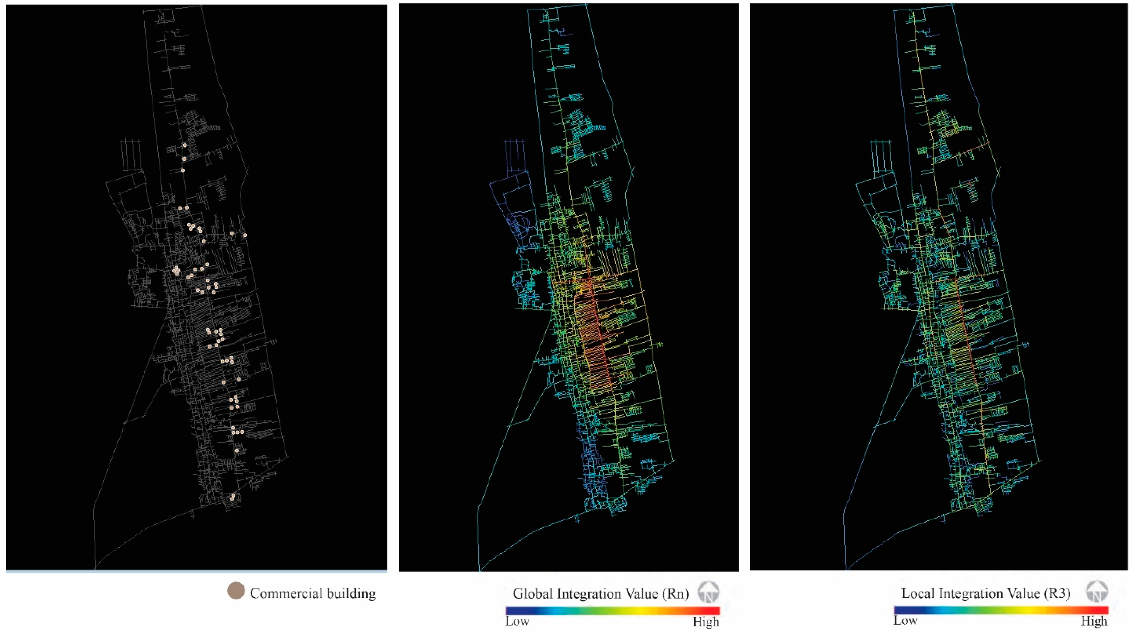
Figure 2.
Physical Vulnerability Index (PVI) Map.
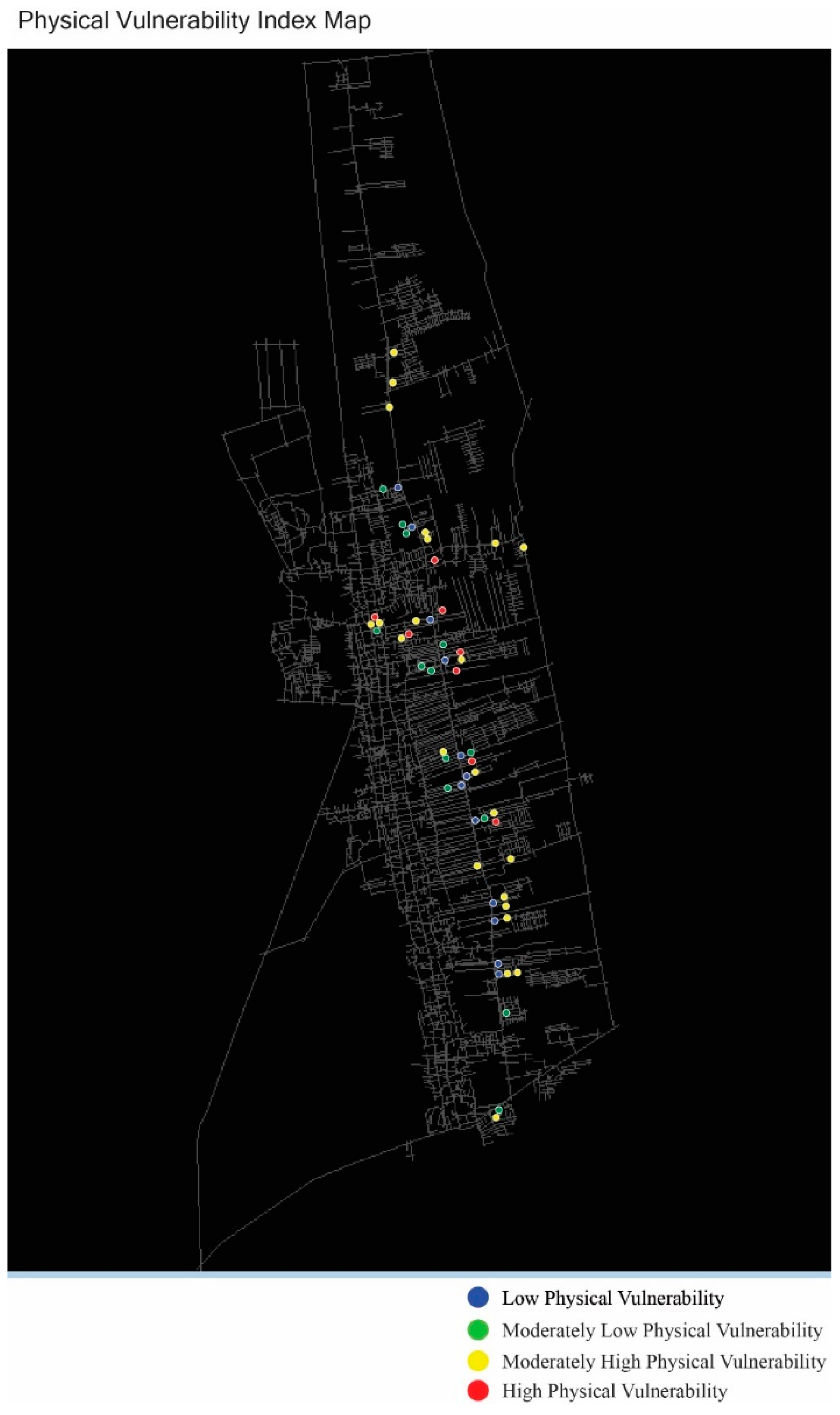
Figure 3.
Physical Vulnerability Index (PVI) at the Low Level.
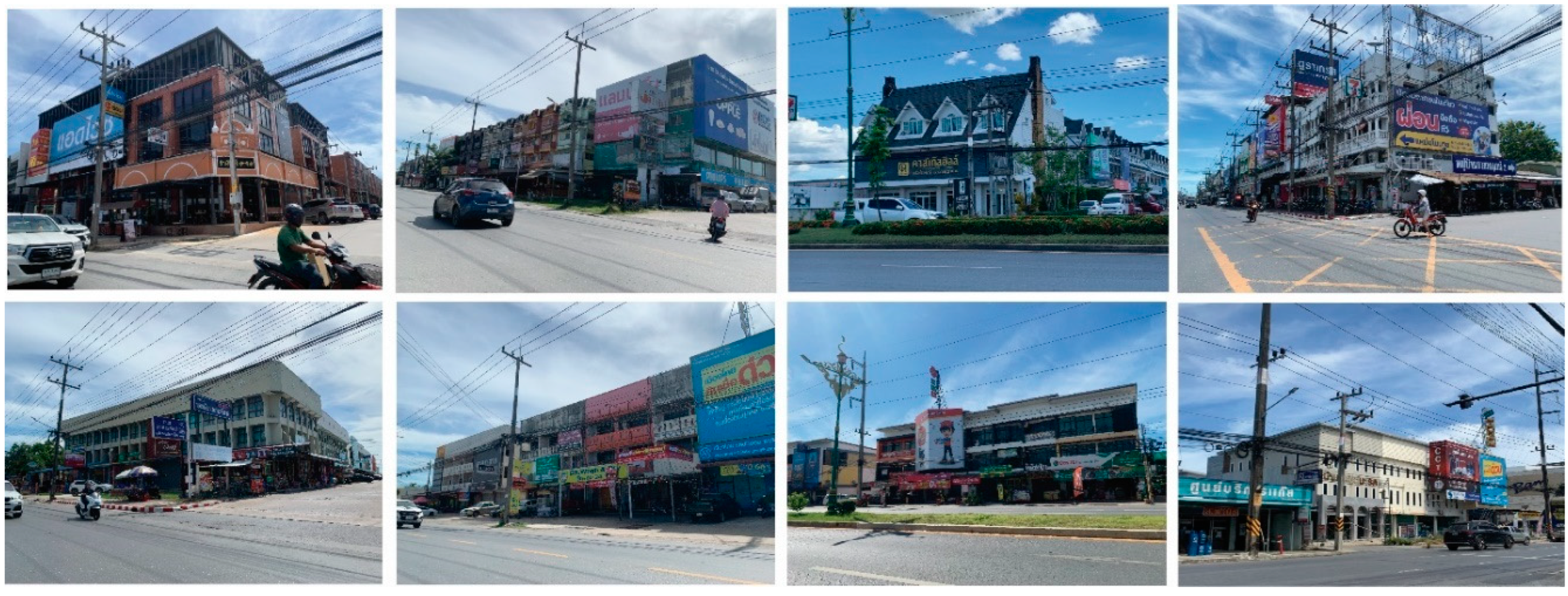
Figure 4.
Physical Vulnerability Index (PVI) at the Moderately Low Level.
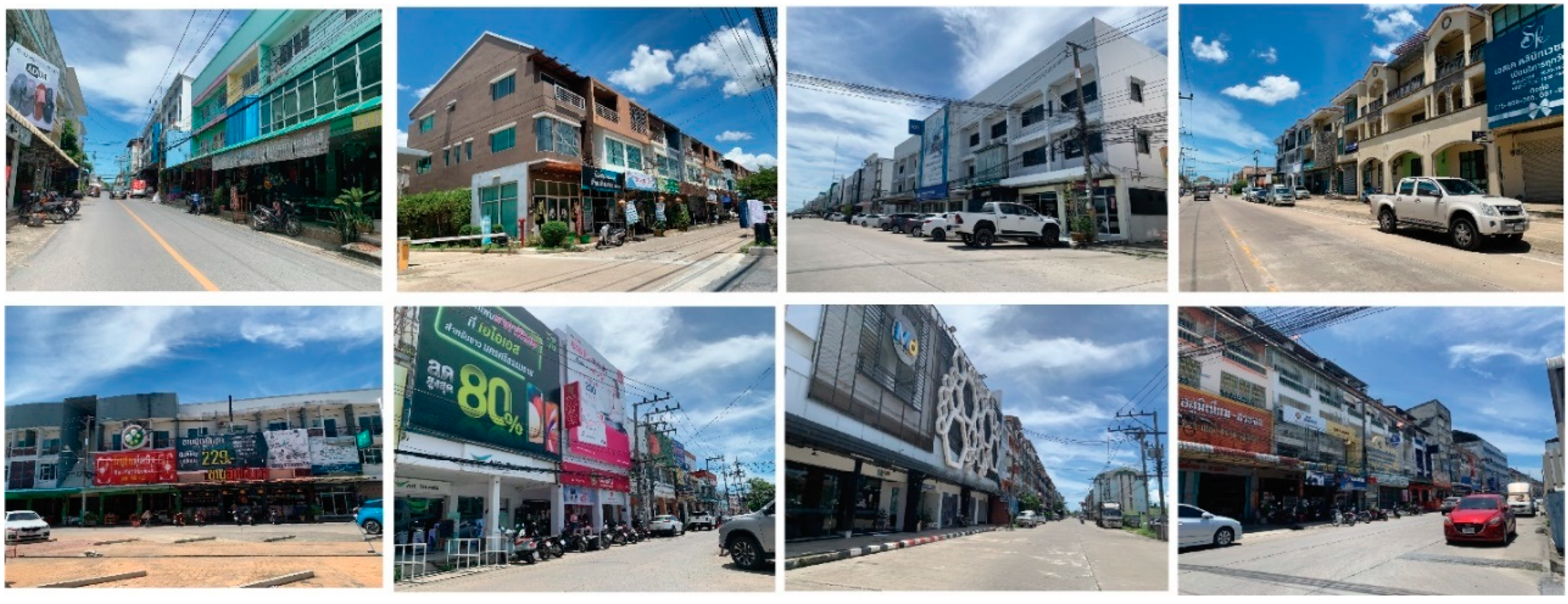
Figure 5.
Physical Vulnerability Index (PVI) at the Moderately High Level.
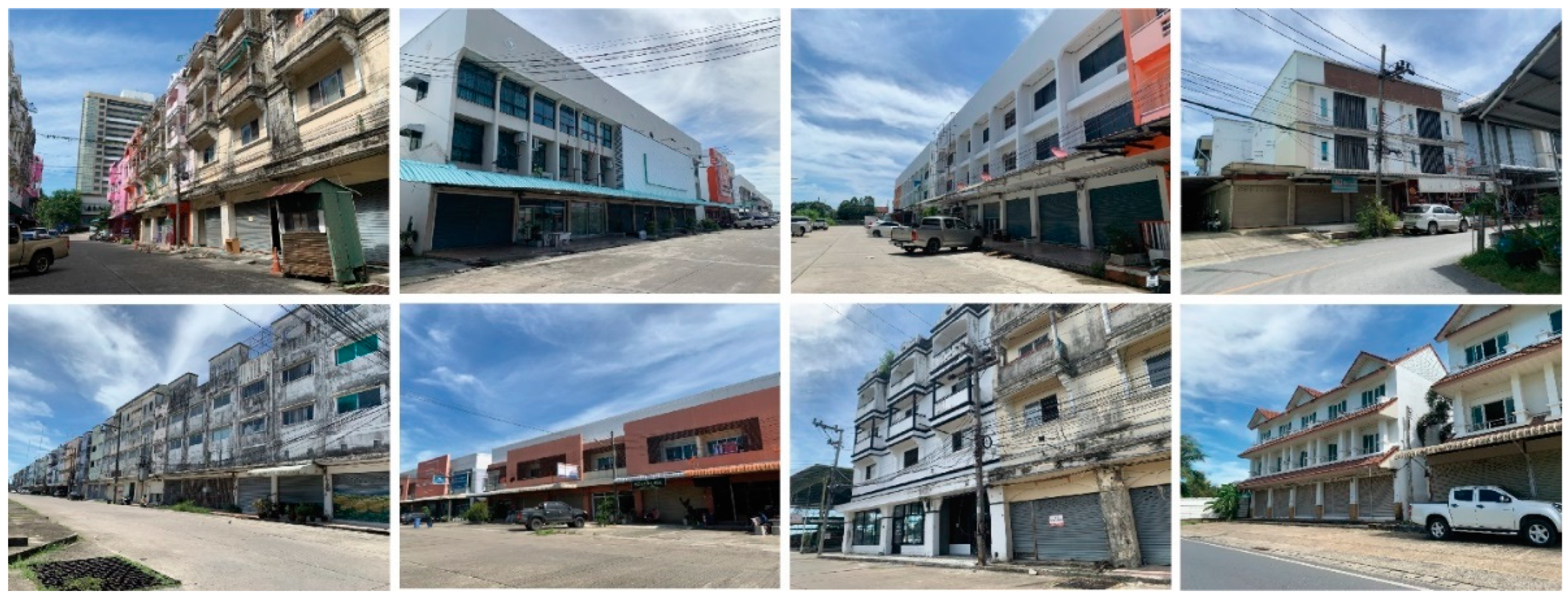
Figure 6.
Physical Vulnerability Index (PVI) at the High Level.
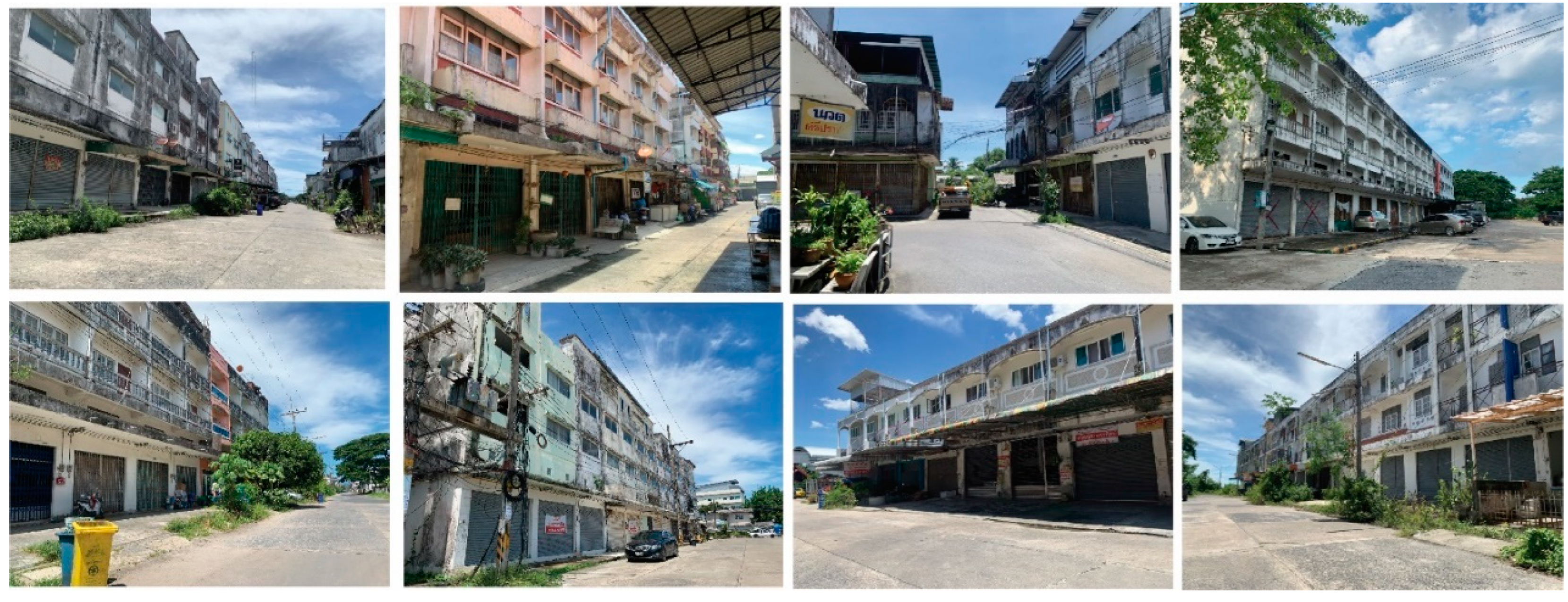

Table 1.
Urban Morphology Variables Determining Physical Vulnerability.
| Urban morphology variables | Variables | Related urban morphology concepts and theories |
|---|---|---|
| 1. Urban Street Networks | 1. Accessibility of Global-level Transportation Projects | Space Syntax Theory, New Urbanism Theory, Eyes on the Street Theory, CPTED Theory, Defensible Space Theory, Space Syntax Theory, Isovist Field Theory |
| 2. Accessibility of Neighborhood-level Transportation Networks | ||
| 2. Public Space Connectivity Patterns | 3. Degree of Depth between the Location and Main Streets | |
| 4. Connectivity of the Location to Main Streets | ||
| 3. Transportation Networks Sustained by Natural Movement of People and Economic Activities | 5. Level of Natural Movement | |
| 6. Commercial Building Usage Rate | ||
| 7. Building Vacancy Rate | ||
| 4. Visibility | 8. Degree of Street Intervisibility | |
| 9. Visibility Potential between the Street and the Building |
Table 2.
Data Collection Methods for Variables Affecting Physical Vulnerability.
| No. | Variables | Values used for analysis | Data collection methods |
|---|---|---|---|
| 1 | Accessibility of Global-level Transportation Networks | Global Integration | Space Syntax Methods: Depthmap Analysis |
| 2 | Accessibility of Neighborhood-level Transportation Networks | Local Integration | Space Syntax Methods: Depthmap Analysis |
| 3 | Degree of Depth between the Location and Main Streets | Mean Depth | Space Syntax Methods: Manual Survey and Calculation |
| 4 | Connectivity of the Location to Main Streets | Relative Asymmetry (RA) | Space Syntax Methods: Manual Survey and Calculation |
| 5 | Level of Natural Movement | Degree of Natural Movement | Gate Count |
| 6 | Commercial Building Usage Rate | Utilization Rate of Commercial Buildings | Survey |
| 7 | Building Vacancy Rate | Vacancy Rate of Commercial Buildings | Survey |
| 8 | Degree of Street Intervisibility | Degree of Street Intervisibility | Manual Survey and Calculation |
| 9 | Visibility Potential between the Street and the Building | Street Width | Survey |
Table 3.
Descriptive Statistics of Variables Affecting Physical Vulnerability.
| NO. | Values used for analysis | N | Minimum | Maximum | Mean | Std. Deviation |
|---|---|---|---|---|---|---|
| 1 | Global Integration | 60 | 0.5343 | 0.9198 | 0.7197 | 0.0956 |
| 2 | Local Integration | 60 | 0.6269 | 3.4588 | 1.9639 | 0.7710 |
| 3 | Mean depth | 60 | 0.0000 | 2.3300 | 1.3148 | 0.6605 |
| 4 | Relative Asymmetry (RA) | 60 | 0.0000 | 1.0000 | 0.3345 | 0.2833 |
| 5 | Degree of Natural Movement | 60 | 2.4800 | 140.6900 | 50.6298 | 37.3138 |
| 6 | Utilization Rate of Commercial Buildings | 60 | 4.0000 | 100.0000 | 56.1610 | 29.9662 |
| 7 | Vacancy Rate of Commercial Buildings | 60 | 0.0000 | 93.7500 | 32.4083 | 25.3156 |
| 8 | Degree of Street Intervisibility | 60 | 0.0600 | 1.0000 | 0.6083 | 0.2845 |
| 9 | Street Width | 60 | 4.0000 | 28.0000 | 10.7666 | 5.3752 |
Table 4.
KMO and Bartlett's Test Results.
| Kaiser-Meyer-Olkin measure of sampling adequacy | 0.817 | |
| Bartlett's test of sphericity | Approx. Chi-Square | 740.130 |
| df | 36.000 | |
| Sig. | 0.000 | |
Table 5.
Rotated Component Matrix (Grouping of Variables Derived from Factor Extraction).
| No. | Variable | Factor Loading | |
|---|---|---|---|
| Component 1 | Component 2 | ||
| 1 | Vacancy Rate | -0.925 | |
| 2 | Degree of Street Intervisibility | 0.924 | |
| 3 | Utilization Rate of Commercial Buildings | 0.898 | |
| 4 | Relative Asymmetry (RA) | -0.847 | |
| 5 | Degree of Natural Movement | 0.817 | |
| 6 | Mean Depth (MD) | -0.657 | |
| 7 | Street Width | 0.634 | |
| 8 | Global Integration | 0.926 | |
| 9 | Local Integration | 0.778 | |
Extraction Method: Principal Component Analysis.
Table 6.
Total Variance Explained.
| Initial eigenvalues | Extraction sums of squared loadings |
Rotation sums of squared loadings |
|||||||
|---|---|---|---|---|---|---|---|---|---|
| Component | Total | % of Variance |
Cumulative % | Total | % of Variance |
Cumulative % | Total | % of Variance |
Cumulative % |
| 1 | 6.230 | 69.227 | 69.227 | 6.230 | 69.227 | 69.227 | 4.986 | 55.399 | 55.399 |
| 2 | 1.112 | 12.356 | 81.583 | 1.112 | 12.356 | 81.583 | 2.357 | 26.184 | 81.583 |
Extraction Method: Principal Component Analysis.
Table 7.
Summary of Variable Grouping Results.
| Component | Variable | Factor loading | Positive/Negative correlation | % of Variance |
|---|---|---|---|---|
| Component 1 |
Vacancy Rate | - 0.925 | Negative | 55.399 |
| Degree of Street Intervisibility | 0.924 | Positive | ||
| Utilization Rate of Commercial Buildings | 0.898 | Positive | ||
| Relative Asymmetry (RA) | - 0.847 | Negative | ||
| Degree of Natural Movement | 0.817 | Positive | ||
| Mean Depth | -0.657 | Negative | ||
| Visibility | 0.634 | Positive | ||
| Component 2 |
Global Integration | 0.926 | Positive | 26.184 |
| Local Integration | 0.778 | Positive |
Table 8.
Descriptive Statistics of Physical Vulnerability Index (PVI) at the Low Level.
| Descriptive Statistics | N | Minimum | Maximum | Mean | Std. Deviation | Ranking |
|---|---|---|---|---|---|---|
| PVScore: Component 1 | 11 | 3.7402 | 4.9321 | 4.523918 | 0.2900815 | Low Physical Vulnerability |
| PVScore: Component 2 | 11 | 0.2482 | 0.9020 | 0.543727 | 0.2645573 | |
| PVI | 11 | 3.9884 | 5.8340 | 5.067664 | 0.4988304 | |
| Z-score_PVI | 11 | 1.3046 | 1.9083 | 1.657636 | 0.1631639 |
Table 9.
Descriptive Statistics of Physical Vulnerability Index (PVI) at the Moderately Low Level.
| Descriptive Statistics | N | Minimum | Maximum | Mean | Std. Deviation | Ranking |
|---|---|---|---|---|---|---|
| PVScore: Component 1 | 15 | 0.2938 | 3.2840 | 1.170807 | 0.8130417 | Moderately Low Physical Vulnerability |
| PVScore: Component 2 | 15 | -0.4213 | 0.4371 | 0.049280 | 0.3035649 | |
| PVI | 15 | 0.0923 | 3.0425 | 1.220100 | 0.9317773 | |
| Z-score_PVI | 15 | 0.0302 | 0.9952 | 0.399113 | 0.3047823 |
Table 10.
Descriptive Statistics of Physical Vulnerability Index (PVI) at the Moderately High Level.
Table 10.
Descriptive Statistics of Physical Vulnerability Index (PVI) at the Moderately High Level.
| Descriptive Statistics | N | Minimum | Maximum | Mean | Std. Deviation | Ranking |
|---|---|---|---|---|---|---|
| PVScore: Component 1 | 26 | -2.7492 | 0.2913 | -1.294754 | 0.8885008 | Moderately High Physical Vulnerability |
| PVScore: Component 2 | 26 | -0.6550 | 0.4247 | -0.228285 | 0.2954769 | |
| PVI | 26 | -2.9462 | -0.0439 | -1.523054 | 0.9485837 | |
| Z-score_PVI | 26 | -0.9637 | -0.0144 | -0.498196 | 0.3102872 |
Table 11.
Descriptive Statistics of Physical Vulnerability Index (PVI) at the High Level.
| Descriptive Statistics | N | Minimum | Maximum | Mean | Std. Deviation | Ranking |
|---|---|---|---|---|---|---|
| PVScore: Component 1 | 8 | -4.9637 | -3.6678 | -4.207662 | 0.5200152 | High Physical Vulnerability |
| PVScore: Component 2 | 8 | -0.5668 | 0.3562 | -0.098150 | 0.3544636 | |
| PVI | 8 | -4.8788 | -3.8826 | -4.305812 | 0.3453469 | |
| Z-score_PVI | 8 | -1.5959 | -1.2700 | -1.408437 | 0.1129653 |
Table 12.
Summary of Components and Spatial Factors Affecting Physical Vulnerability.
| Component | Factor | Characteristics of Physical Vulnerability |
|---|---|---|
| Component 1 Micro-level Morphological Structure | 1. Configuration of Space | Non-distributed street network; dead-end or cul-de-sac streets |
| High depth between the location and main roads | ||
| Low street intervisibility | ||
| 2. Characteristics and Rate of Space Utilization | High building vacancy rate | |
| Low street intervisibility | ||
| Low level of natural movement | ||
| Component 2 Macro-level Morphological Structure | 1. Accessibility of Global-level Transportation Networks | Low accessibility of global-level transportation networks |
| 2. Accessibility of Neighborhood-level Transportation Networks | Low accessibility of neighborhood-level transportation networks |
Disclaimer/Publisher’s Note: The statements, opinions and data contained in all publications are solely those of the individual author(s) and contributor(s) and not of MDPI and/or the editor(s). MDPI and/or the editor(s) disclaim responsibility for any injury to people or property resulting from any ideas, methods, instructions or products referred to in the content. |
© 2025 by the authors. Licensee MDPI, Basel, Switzerland. This article is an open access article distributed under the terms and conditions of the Creative Commons Attribution (CC BY) license (http://creativecommons.org/licenses/by/4.0/).
Copyright: This open access article is published under a Creative Commons CC BY 4.0 license, which permit the free download, distribution, and reuse, provided that the author and preprint are cited in any reuse.


