Submitted:
18 April 2025
Posted:
21 April 2025
You are already at the latest version
Abstract
We propose a unified geometric framework in which space and time emerge as observer-dependent projections of quantum correlations embedded in the universal wavefunction. In this approach, we formulate six axioms (including a duality between entanglement and time) that establish a correspondence between correlation structures and effective spacetime geometry. We introduce the "correlationhedron", a convex geometric object representing the set of all permissible correlation vectors of a given state, and show how different observer "slicings" (modeled by projection maps) yield distinct emergent spacetimes from this object. An emergent metric is defined on each observer's spacetime via the second derivative of a correlation density (analogous to a Fisher information metric), linking gradients in quantum entanglement to curvature. This paper establishes the conceptual foundations of this approach as the first in a planned series of investigations. We illustrate the framework with conceptual and quantitative examples, including an explicit calculation of the emergent geometry for a two- qubit system in both separable and entangled states. Connections to holography (AdS/CFT) (Maldacena1998, Ryu2006), tensor networks (Swingle2012), and relational quantum approaches (Rovelli1996) are discussed, along with experimental signatures (such as curvature variations with entanglement) that could support the theory. Finally, we outline the limitations of the framework, particularly regarding dynamics and observer-dependent causality, to guide future investigations. This kinematic framework establishes the conceptual skeleton of emergent spacetime; detailed constructions, proofs of smoothness, and dynamical laws will appear in forthcoming work.
Keywords:
Quantum correlations
; Emergent spacetime
; Correlationhedron
; Entanglement-time duality
; Quantum geometry
; Observer-dependent reality
; Information geometry
; Holographic principle
; Tensor networks
; Quantum foundations
1. Introduction
1.1. Motivation and Overview
The nature of space and time remains one of the central puzzles in modern physics. In the prevailing paradigm, general relativity treats spacetime as a dynamical continuum curved by energy and momentum, whereas quantum mechanics relies on the wavefunction to describe probabilistic outcomes of measurements. An emerging perspective—fueled by insights from quantum gravity and quantum information—posits that space and time are not fundamental but instead emerge from deeper quantum correlations[5]. In this work, we propose that the universal wavefunction contains a high-dimensional web of quantum correlations, and classical space and time arise as observer- dependent projections of this underlying structure. This paper presents the foundational framework and conceptual machinery for this approach, establishing a program for further investigation that we intend to develop in subsequent work. We introduce the concept of a correlationhedron (denoted ): a convex set encompassing all physically consistent correlation vectors derivable from . We show how different “slicings” of —corresponding to different observers or reference frames—recover familiar aspects of spacetime geometry (such as locality and curvature). This observer-dependent perspective is reminiscent of the Heisenberg cut in quantum mechanics – the notional boundary between the observer and the system. In our context, each choice of observer effectively places such a cut, isolating a subset of the universal correlations as that observer’s experienced spacetime. Drawing parallels with ideas from information geometry and entanglement renormalization, our aim is to unify quantum mechanical and gravitational phenomena under a common, correlation-centric framework.
Notably, while our correlationhedron shares a geometric spirit with concepts like the entanglement polytope from quantum information theory, it differs significantly in scope, structure, and applicability. The entanglement polytope (e.g., [6]) describes the set of possible one-body marginal eigenvalues (entanglement spectra) achievable by states within a given entanglement class, whereas captures the full range of correlation patterns (including multi-partite and temporal correlations) for a fixed state . In other words, is a state-specific, high-dimensional object encompassing much richer information than the limited local marginals summarized by entanglement polytopes. Moreover, is utilized here to derive an emergent spacetime geometry for each observer. This is an application beyond the purview of entanglement polytopes, which have primarily been used to classify entanglement types. This distinction underscores the novelty of the correlationhedron concept within our framework.
1.2. Recent Developments
Our proposal builds on a variety of modern approaches linking geometry and quantum correlations. For instance, the AdS/CFT correspondence1[1] demonstrates how entanglement entropy can be used to reconstruct higher-dimensional geometry[2,7]. Tensor-network descriptions like MERA2[8,9] highlight how renormalization-group flow encodes emergent spatial structure. Notably, Van Raamsdonk has argued that progressively increasing entanglement between two halves of a divided quantum system causes their dual spacetime regions to join together, whereas removing entanglement can tear spacetime apart – a dramatic illustration that entanglement is the “glue” of spacetime[10,11]. At a more combinatorial level, geometric objects such as the amplituhedron provide striking examples of how scattering amplitudes can be organized in a purely geometric fashion[12].
It remains an intriguing open question whether the amplituhedron itself can be realized as a state-specific correlationhedron. Concretely, one would seek a quantum state (for instance, the planar SYM vacuum) and a set of operators whose two-point or higher correlators furnish precisely the momentum-twistor data of the amplituhedron. If the allowed region of these correlators coincided with the amplituhedron and the push-forward of the natural volume on reproduced the canonical form of the amplituhedron, then scattering amplitudes would emerge directly from quantum-state correlations. We view this as a promising direction for future work.
Finally, studies of entanglement area laws in many-body systems[13] and relational quantum gravity models[14] lend support to the notion that classical spacetime can arise from underlying quantum informational degrees of freedom.
The framework presented in this paper should be understood as a conceptual foundation rather than a complete theory. We establish the basic mathematical structures and relationships while identifying the key questions that must be addressed in developing a full theory of emergent spacetime from quantum correlations. Subsequent work will focus on expanding the mathematical rigor, addressing dynamical aspects, and exploring more complex systems beyond the toy models presented here.
1.3. Completeness and Positivity
- Axiom A1 (Completeness): All physically realizable correlations of the universal wavefunction can be embedded in the correlationhedron . This echoes the holographic idea that every degree of freedom of the state is encoded in its correlation structure [15].
- Axiom A2 (Positivity): Quantum correlations are derived from positive semidefinite operators. For example, for any observables and ,which implies that the covariance matrix is positive semidefinite. This ensures that is a convex set [16].
1.4. Observer Slicability and Locality Emergence
- Axiom A3 (Observer Slicability): An observer, by choosing a set of measurements, projects onto a lower-dimensional manifold . This projection, denoted , is determined by the observer’s frame (e.g., their velocity or measurement basis) and is responsible for the emergence of effective spacetime [7].
- Axiom A4 (Locality Emergence): In sufficiently localized regions of , correlations cluster such that an approximate notion of locality arises. This is in accord with area-law behaviors observed in low- energy states [16].
1.5. Curvature from Gradients and Entanglement–Time Duality
- Axiom A5 (Curvature from Gradients): Variations in the quantum correlation density induce effective curvature in the emergent spacetime. Steep gradients in the correlation distribution act analogously to mass-energy in classical general relativity, curving the effective geometry (requires and bounded in local patches).
-
Axiom A6 (Entanglement–Time Duality): Temporal ordering and quantum entanglement are two complementary manifestations of the same underlying correlation structure (strictly holds when factorizes as ; see Page–Wootters [17]). For example, in the Page–Wootters mechanism3[17], entanglement between a clock and a system gives rise to time evolution. Here, the observer’s projection can turn entanglement into an emergent temporal ordering. For instance, consider a global state of the formAn observer with access only to the system (but not the clock) perceives the sequence as a time-ordered evolution. Thus transforms the clock-system entanglement into an emergent time coordinate t.
These axioms establish the idea that the full set of quantum correlations (encoded in ) can be partitioned by an observer into an emergent spacetime, where the structure and geometry are intimately tied to the state’s correlation patterns.
While this initial framework primarily addresses kinematic aspects, it provides the necessary foundation for exploring dynamical features in future developments. The axioms themselves suggest natural extensions to temporal evolution that will be explored in subsequent work.
2. Mathematical Framework
In this section we translate the axioms into a concrete mathematical construction. We define the correlationhedron more formally, describe how an observer’s projection produces an effective spacetime manifold, and derive an emergent metric on that manifold.
To formalize this slicing process, we introduce the notion of an observer projection:
Definition 2.1
(Observer Projection). An observer projection is a smooth map from the full correlation structure to a lower-dimensional manifold , representing the effective spacetime experienced by an observer . Formally,
This map selects the subset of observable correlations accessible to the observer, typically by restricting to a subalgebra . The image inherits coordinates corresponding to expectation values of observables in , and geometric structure is induced via correlation densities on .
2.1. Correlationhedron Definition and Convexity
Let be the Hilbert space of a closed quantum system described by the wavefunction (or a density matrix for a pure state, generalizable to mixed states). We define the correlation space as the space of all possible correlation vectors that can be constructed from expectation values of products of observables on the system. Each is of the form:
for some choice of N observable pairs (these could be, for example, all distinct pairs of a chosen operator basis on ). Not all vectors in are allowed; only those obeying quantum constraints (linearity, positivity, etc.) correspond to a physical state.
For a specific state (or ), we define the correlationhedron:
In words, is the set of all correlation vectors attainable by the system when it is in the state (allowing variation over different measurement contexts or decompositions but not over different states) [18]. By construction, each arises from a positive semi-definite (Axiom A2), hence is a convex set [19].
This convexity follows directly from the linearity of expectation values in . For any two states and ,
so any convex combination of correlation vectors remains in .
In this paper, for concreteness, we restrict correlation vectors to include all two-point correlators drawn from a chosen operator basis on . Extensions to higher-order and temporal correlations, while straightforward in principle, are deferred to future work.
The term “hedron” highlights that is a geometric object (indeed, typically a convex polytope or a curved convex body) in the high-dimensional space of correlations. This construction is reminiscent of the amplituhedron in particle physics [20], which is a convex geometric object encoding scattering amplitudes. Likewise, encodes quantum correlation data in a single geometric entity.
can be thought of as living in a high-dimensional space, whose dimensionality is determined by the number of independent correlation components one considers. In practice, symmetries or selection of particular observable sets can reduce this dimensionality. For example, for a system of many qubits, one might consider the set of all two-point correlators (with labeling qubits and Pauli components). The collection of these for all gives a correlation vector. The set of all such vectors physically achievable by a given would form . By Axiom A1, is assumed to capture all relevant correlations of the state.
Concretely, given an observer whose accessible observables are , the projection map acts by selecting the subvector
where indexes the observables available to that observer. Thus
is the restriction of correlation vectors to the observer’s measurement subspace.
This construction may be viewed as a vast generalization of the classical correlation polytope studied in quantum foundations. In particular, Pitowsky’s Bell-scenario polytope characterizes the set of all joint probability assignments compatible with local hidden–variable models [21], and the Tsirelson bounds constrain its quantum-mechanical analogue by imposing operator-positivity and commutation relations [22]. By contrast, the correlationhedron encompasses all two-point—and, in principle, higher-order and temporal—correlations arising from a single global state . Whereas the Bell polytope is carved out by linear constraints on measurement outcomes in a fixed spacelike configuration, is defined by the full family of operator covariance relations,
and is automatically convex by positive-semidefiniteness of the density operator. Moreover, by allowing to come from different times—as in temporal correlations à la Leggett–Garg—this framework extends beyond the purely spatial scenarios of Bell tests, yielding a unified geometric object for arbitrary observables and spacetime orderings.
In the following sections, we first explore how an observer’s projection gives rise to an emergent spacetime (Section 2.2), then formalize the mathematical structure and admissibility conditions of these projections (Section 2.3), and finally derive how such projections yield a geometric structure (Section 2.4–2.6).
2.2. Examples and Intuition for Observer Projections
While represents the totality of correlations in the quantum state, an observer can only access a subset of this information. We model the perspective of a given observer by an observer projection mapping
which takes the full correlationhedron and produces a lower-dimensional “shadow” of it on an effective manifold [12]. Here is a manifold (with dimension d typically much smaller than that of ) that the observer interprets as their physical space and time. We furthermore assume (three spatial coordinates plus one time coordinate). In practice, Axiom A4 (locality emergence) and Axiom A6 (entanglement–time duality) guide the choice of observables so that can be interpreted as a classical 3+1-dimensional spacetime for the observer. The parameter denotes the observer’s state (for example, could encode the observer’s velocity, orientation, choice of measurement basis, or other contextual information).
If the observer’s subalgebra has a nondegenerate reduced state and its expectation values vary smoothly with the global state , then there exists a smooth projection map
whose Jacobian has full rank almost everywhere on .
In general, will be a many-to-one map (different points in may look identical to a given observer if they cannot be distinguished by that observer’s measurements). A simple example of a projection is to marginalize over (i.e. ignore) certain correlation components. For instance, an observer might be sensitive only to two-point correlations among a subset of particles, and blind to higher-order correlations or correlations involving other distant particles. In that case, could be a linear projection picking out those two-point correlators from the full vector . Another example: if the observer moves at high velocity, their notion of simultaneity changes (relativistic time dilation), which in this framework could correspond to a different slicing through correlation time-orderings in .
Importantly, should be chosen such that the image inherits meaningful coordinates interpretable as space and time for the observer. (One might need additional structure to define a metric or geometry on , but we address that shortly.) There may not be a unique way to choose — indeed, there are many possible ways to define an observer’s slice[23]. However, Axiom A3 demands that some consistent projection exists for any valid observer.
Clarification (Examples of ): To build intuition, consider two extreme cases of projections. At one extreme, an “ideal” observer with access to all degrees of freedom would have as the identity on , recovering the full structure (and thus presumably a high-dimensional, highly curved space). At the other extreme, a very limited observer who can only measure one variable might map to a 1D manifold (just the expectation value of that variable), losing most of the structure. Realistic observers lie in between, projecting out some but not all information. The choice of can be dynamic — for instance, an accelerating observer might effectively change their projection over time.
While multiple distinct projections can map to observationally equivalent spacetimes, any physically relevant distinction must be empirically accessible through measurement outcomes.
2.3. Mathematical Structure of Observer Projections
Let be the Hilbert space of the quantum system with global state (or pure state ). Let be the full observable algebra on , and let be the subalgebra accessible to an observer labeled by parameter .
Define the space of two-point correlators:
Define the correlationhedron for a fixed state as:
We model an observer’s emergent spacetime via a projection map:
where selects a subvector of correlators for some finite index set .
Definition (Admissible Projection): A projection is admissible if it satisfies:
1. Positivity Preservation: is positive semidefinite. 2. Smoothness: is at least smooth on , i.e., all derivatives up to second order exist. 3. Full Rank: The Jacobian of has full rank almost everywhere.
Proposition: If is a -smooth density operator and is finite-dimensional with smooth matrix elements, then is admissible.
2.4. Emergent Metrics from Correlation Densities
Given a particular observer’s projected manifold , we must define how this manifold inherits a notion of distance or metric from . A natural approach is to introduce a correlation density on that captures how densely correlations from map to different regions of .
Note that
so one may equivalently write the metric as
See Appendix A.2 for a detailed discussion of this sign convention. By construction, the emergent metric is positive-definite, thus defining a Riemannian metric on . This guarantees all observer-defined distances are real; the conditions for the emergence of a Lorentzian signature (with light-cone structure) will be sketched below. The emergent metric encodes the curvature of the effective spacetime manifold through variations in the density of correlations. Regions of steep changes in correlation density correspond to higher curvature. Here is the density induced on by projecting the natural volume on through , so that equals the volume of its preimage in .
This coincides with the Fisher information metric on the statistical manifold defined by (see Appendix A.2 for derivation).
Intuitively, if a particular region of corresponds to many distinct points in (i.e., many different underlying correlation configurations look the same to the observer), then in that region is high. Conversely, if very few configurations project to a region, is low.
From , we can recover the emergent metric tensor on ((see Eq. (2)), which is analogous to the Hessian of the negative log density [24]. Equivalently, is the Fisher-information metric tensor if we treat as defining a statistical manifold. This choice ensures several desirable properties:
- It is manifestly observer-dependent. Different yield different and thus different metrics. This aligns with the idea that geometry is not absolute but tied to the observer’s slicing of correlations.
- It is positive-definite (so long as in the neighborhood, ensuring no singular behavior in the log-density). This means distances computed from are real.
- It responds to correlation gradients: regions where changes rapidly will have a large curvature (as second derivatives are large), while flat regions of give flat geometry.
A key requirement for to serve as a Riemannian metric is that it be nondegenerate (invertible) everywhere on . This will be true if is smooth and nowhere vanishing on (or more precisely, may approach zero but not be identically zero in a patch, so that is well-behaved). In practice, might be very small or zero in some regions if certain correlation configurations are impossible or extremely unlikely for a given . In those cases, the metric may become singular, signaling an “edge” to the observer’s spacetime (beyond which no points from map). Physically, this could correspond to horizons or singularities from the observer’s perspective, beyond which their measurements cannot probe.
This emergent metric encapsulates how the observer perceives distances in their space in terms of underlying correlation configurations. If is uniform, is zero (flat space) – meaning the observer sees no curvature, as every region of their space corresponds to equally many underlying configurations. If is sharply peaked in one area and shallow in another, will vary across , indicating curvature (the observer might interpret that as a gravitational field or tidal force in their space). In essence, areas of high correlation density act like “mass” – they pull the geometry tight (high curvature), whereas sparse regions act like voids (flat or even effectively negative curvature in a relative sense if we allowed an analogy to negative mass).
2.5. Conditions for Lorentzian Signature
While this emergent metric is initially Riemannian (positive-definite), the structure naturally generalizes to include time-like directions and causal ordering. In particular, a Lorentzian signature may arise by partitioning correlation density into temporal and spatial components. This provides a bridge between statistical curvature and relativistic geometry. To obtain a pseudo-Riemannian metric with one time-like direction, one can split the projection into clock and spatial pieces:
then define:
This yields a signature (when and satisfy differentiability and positivity conditions), consistent with the standard Lorentzian structure of spacetime, while the underlying correlation space remains positive-definite. The negative sign associated with the temporal derivative reflects the causal distinction between time-like and space-like directions, ensuring that the emergent geometry preserves conventional causal structure. We leave the explicit construction of such a projection to future work.
In practice, identifying and depends on the observer’s clock–system decomposition or symmetry properties of the state, as discussed in relation to Axiom A6 and the Page–Wootters construction. This decomposition presumes that observer-accessible correlations can be naturally partitioned into temporal and spatial sectors, such as when the clock–system factorization is approximately valid or when the state exhibits symmetry under time translations. In principle, regions where the sign of the log-derivative flips could signal transitions between Riemannian and Lorentzian character—an idea reminiscent of signature change in certain quantum cosmological models.
2.6. Curvature and Observers’ Perspectives
How does this formal emergent curvature relate back to known physics? If is indeed to be interpreted as an observer’s spacetime, then variations in should mimic gravitational effects for that observer. In our construction, steep gradients in play the role of energy density in general relativity, curving . For example, if has a pronounced peak (indicating a cluster of correlations concentrated in one region of ), the Hessian will be large there, meaning a strong curvature. An observer might interpret that as a massive object creating gravitational attraction in that region. Conversely, if is nearly flat, is nearly flat.
We emphasize that this metric is emergent and state-dependent. Change the quantum state , and changes, changes, and thus the geometry on changes. This provides a concrete implementation of the idea that spacetime (and its curvature) is not fundamental, but arises from the quantum state’s correlations.
To draw a parallel, consider how in the AdS/CFT correspondence entanglement entropy in the boundary theory relates to the geometry of the bulk spacetime (via the Ryu–Takayanagi formula). In our framework, is a more fine- grained object than entropy – it’s a distribution capturing the full spectrum of correlations, not just the entropy. Yet it plays a somewhat analogous role, dictating the emergent geometry. Where AdS/CFT uses minimal surfaces to probe bulk geometry (with areas corresponding to entropies), here we use correlation densities to directly shape the metric. Importantly, our approach does not assume any pre-existing spacetime such as AdS; it applies to an arbitrary state .
Finally, one might wonder: do all choices of lead to a reasonable geometry? Perhaps not. Some projections might yield a highly singular or otherwise pathological metric. In such cases, the resulting fails to be a well-defined differentiable manifold. This is not unexpected – not every arbitrary slicing of correlations will correspond to a semi-classical spacetime. The hope, however, is that for “natural” choices of observables (the kind an actual physical observer might have access to), will be well-behaved. In the Appendix A.1, we discuss some conditions for the existence and smoothness of and how to handle cases where the emergent metric might become degenerate or singular.
In summary, the emergent metric on provides the observer’s “gravitational field”: it tells them how their space stretches or compresses in different regions as a function of the underlying quantum state’s correlation distribution. Curvature in this space is directly tied to inhomogeneities in – which are, in turn, features of ’s correlation structure. Thus, in our approach, gravity is nothing but the second derivative of the log correlation density: a statement that is reminiscent of, but more general than, entropic gravity proposals.
We will next illustrate these ideas with simple toy models, to see explicitly how entanglement (or lack thereof) in leads to a particular and for an observer.
We now extend the static picture by considering how a time-evolving quantum state induces a trajectory through the correlation space , leading to a time-dependent emergent geometry for the observer.
2.7. State Trajectories and Time-Dependent Correlation Geometry
So far, we have focused on static correlations and emergent geometry from a fixed state. In this section, we explore how time-evolving quantum states induce dynamics on the emergent manifold.
Let the global state evolve unitarily:
for some Hamiltonian H. Then is a time-dependent convex set.
Let be the time-dependent correlation density on defined by:
where is a measure on and * denotes the pushforward.
Define the emergent metric at time t by:
Then the emergent Ricci tensor can be written as:
These curvature terms may include mixed partial derivatives or non-Hessian contributions, depending on the underlying geometry of .
We conjecture a dynamical law:
where is a functional of and its derivatives, acting as an effective energy-momentum tensor from quantum correlations.
3. Conceptual Toy Models
To build intuition, we examine a few toy models that illustrate how the abstract machinery of the correlationhedron and observer projections works in simple settings. These examples highlight how locality, curvature, and entanglement– time duality manifest in concrete quantum systems.
3.1. Single-Qubit Temporal Correlations
Our first toy model is a single qubit (two-level quantum system) observed over time. Even though a single qubit has no spatial extent, it can illustrate the entanglement–time duality (A6) in a trivial setting by considering correlations in time.
Consider a qubit initially prepared in state and then measured at two different times (by the same observer). The correlationhedron in this case could be taken as the set of all two-time correlation values for observables at times and . If the qubit’s Hamiltonian is H, its state evolves as . Suppose the observer measures at time and at time . We can talk about a correlation which will depend on the initial state and the time difference . In this simple case, might be one- dimensional (since essentially one parameter controls the correlation).
According to our framework, the observer (here implicitly at rest relative to the qubit) projects onto a 1D manifold which we can identify with the time axis itself.
The correlation density on this time axis could be related to how correlation varies with . For example:
- If is an eigenstate of , thenso is uniform (flat emergent time).
- If is a superposition, thengiving a peaked near that decays for larger . The emergent metric then varies, producing segments of different “length.’’
The main takeaway from the single-qubit example is that even temporal correlations of a single degree of freedom can be seen as defining an emergent time dimension. The entanglement–time duality is trivial here (no entanglement since one qubit, but the role of correlation in time is analogous to entanglement in space for larger systems). This sets the stage for considering space and time on equal footing as two ways of slicing correlation structures.
3.2. Two Qubits: Entangled vs. Separable
A more illuminating toy model is a two-qubit system, which we can use to explicitly demonstrate how entanglement generates curvature in the emergent geometry (A5) and how locality emerges (or fails to) depending on the state.
For our two qubits (call them A and B), consider two extreme initial states:
- A separable state, e.g. , which has no entanglement between qubits A and B.
- An entangled state, e.g. the Bell state , which possesses maximal entanglement between A and B.
We will examine each case through the lens of our framework, determining on an appropriate and the resulting curvature.
For simplicity, let us define our observer’s projection such that captures an effective one-dimensional “distance” between qubits A and B. Imagine the observer only measures two-qubit correlation functions that have a notion of spatial separation – for instance, they might look at correlators of the form , and we interpret the strength of correlation as an inverse distance.
One way to do this is to define a proxy for distance ℓ via the correlation between spins along a certain basis. Suppose our observer measures both z-z correlations and x-x correlations . Intuitively:
- If both z-z and x-x correlations are high (close to +1 or –1), it suggests the qubits are “locked together’’ in all measured orientations – we interpret this as the qubits being effectively at zero separation (a single combined object).
- If correlations are low or depend on orientation, the qubits behave more independently – we interpret this as some distance between them.
Let’s quantify an effective separation ℓ such that corresponds to maximal correlation in all bases, and larger ℓ corresponds to weaker or basis-dependent correlations. A brief sketch of the exact push-forward measure is as follows. Define
and set . Then
where is the natural volume on . We then adopt a Gaussian proxy
(see Eq. 4) for intuition.
For the separable state : - (since both spins are up in z). - Since the product state factorizes, one has
as each qubit in satisfies . So in one basis the qubits appear perfectly correlated, and in another they are uncorrelated. The observer would conclude that A and B are not one single object – there is some “distance” between them that allows them to behave independently in at least one measurement basis. for the separable state might be relatively broad, reflecting that the two qubits do not share a close locality in the emergent picture.
For the Bell state : - (since half the time both are up, half both are down). - as well (the Bell state is also an eigenstate of with eigenvalue +1). In fact, all corresponding two-qubit correlators in orthogonal bases are +1 for this Bell state. The observer sees A and B perfectly correlated in every way they check. The natural interpretation is that : the qubits are at the same “location’’ in the emergent space (or even considered a single entity). The correlation density would then be sharply peaked at .
We can illustrate the effective correlation density for the two cases:
A simple ansatz for the correlation density as a function of the effective separation ℓ is
Here, denotes the characteristic correlation length scale. Hence, from Eq. (2), and using the Gaussian ansatz in Eq. (4), the emergent metric component becomes
In summary, the two-qubit toy model shows that:
- When two systems are entangled, an observer’s emergent space will tend to place them close together with a non-trivial geometry (possibly high curvature or even effectively identifying them as a single point for maximal entanglement).
- When two systems are not entangled, it is possible for an observer to find a frame where they appear entirely uncorrelated (far apart, no direct influence), reinforcing the emergent locality.
This provides a concrete demonstration of both locality emergence and curvature-from-correlation using the simplest non-trivial quantum system.
3.3. Observer-Dependent Outlook
Finally, we emphasize the observer-dependent aspect using a slight variation of the two-qubit scenario. Imagine two observers looking at the same two- qubit entangled state , but choosing different measurement contexts:
- Observer Alice measures correlations.
- Observer Bob measures correlations (mixing bases between qubits).
Alice, as we saw, finds for the Bell state, and also (if she also measured x-x). So in Alice’s chosen basis set, A and B appear tightly bound with maximal correlation in both directions she checks.
Bob, however, measures A in z and B in x. For , what is ? One can compute this: for this state (because the Bell state is symmetric under simultaneous rotations, but if you measure different axes, correlations can cancel out). In fact, on A and on B anticommute on the state in a way that yields zero expectation. So Bob would observe no correlation in his chosen observable pair. To Bob, it might appear that the two qubits are not directly correlated (since whenever A is up or down, B is equally likely to be + or − in x). Thus, Bob’s emergent picture might place the qubits as more distant or even disconnected along the axis he’s examining.
This situation encapsulates the relativity of correlations: The “distance” or “connection” between two subsystems in the emergent space is not absolute, but depends on how the observer probes them. Alice’s projection yields a geometry where A and B are at zero separation (a single coupled system), whereas Bob’s projection —slicing differently—yields a geometry where A and B seem separated (at least in one direction of his space). Neither is wrong; they are simply different lower-dimensional views of the same . Of course, if an observer has access to all possible measurements (full tomography of the two-qubit state), they would reconstruct the full and recognize the state as entangled. But practical observers are limited, which is one reason different reference frames (or observers) can have different “slices” of reality.
To the extent that a shared consensus reality exists, it would emerge when observers compare notes and effectively combine their correlation data. But as long as they are looking at different cross-sections of , their personal geometries can differ — a nod to relational quantum mechanics interpretations where facts are observer-dependent.
From the two-qubit example and this observer-dependent twist, we see how the same quantum state can give rise to different emergent spacetimes for different observers. Entanglement (or the lack thereof) informs curvature, and the choice of measured observables informs the notion of distance and connection. This paves the way for exploring larger systems where these ideas might play out in more complex and rich ways, as we will discuss in the context of holography and other paradigms.
4. Connections to Existing Paradigms
4.1. Relation to AdS/CFT and Holography
One of the strongest pieces of evidence that spacetime geometry and quantum entanglement are closely related comes from the Anti-de Sitter/Conformal Field Theory (AdS/CFT) correspondence4[1]. In holographic duality, a -dimensional gravitational spacetime in AdS is dual to a d-dimensional quantum field theory on the boundary. Crucially, entanglement entropy in the boundary theory is connected to the area of extremal surfaces in the bulk spacetime via the Ryu–Takayanagi formula[2]. In other words, entanglement (a quantum information quantity) directly gives rise to a geometric object (an area) in a higher dimension. This has led to slogans like “Entanglement builds geometry’’[7].
Our correlationhedron framework is in harmony with these ideas. Here, the entire set of correlations plays a role reminiscent of the AdS bulk, and an observer’s spacetime is like a slice or patch of that bulk corresponding to a particular “code subspace’’ or perspective. A large entanglement between two parts of the boundary CFT (say two halves of the system) corresponds to those parts being connected in the bulk — potentially even by a wormhole if the entanglement is maximal (as conjectured in ER=EPR[10,11]). In our model, a maximally entangled pair of subsystems would appear as a single unified region in an observer’s , analogous to how two black hole boundaries connected by a wormhole represent one geometry. Van Raamsdonk’s thought experiment[7], where gradually reducing entanglement causes spacetime to “split’’ into two disconnected pieces, has a direct parallel: in the correlationhedron, if correlations between two sectors shrink, the projection for an observer can make those sectors drift apart in the emergent space (potentially becoming separate spacetimes if entanglement goes to zero).
Another point of contact is the idea of the entanglement wedge in holography. The entanglement structure of a region of the CFT determines a certain bulk region (its entanglement wedge). In our terms, picking a particular observer (who might correspond to having access to only a region of the full system’s degrees of freedom) will project onto a certain that might correspond only to that wedge. While our framework is more general (not relying on a pre-existing spacetime, and not limited to conformal or highly symmetric states), it is encouraging that it reproduces the qualitative dependence of geometry on entanglement seen in AdS/CFT[7,10].
In summary, the correlationhedron approach can be seen as a generalization of holographic ideas beyond AdS backgrounds: any quantum state has a “bulk’’ of correlations, and any observer provides a “boundary’’ description (with one lower dimension) that experiences a geometry. When the state in question happens to be one like those in AdS/CFT (highly entangled, obeying area laws, etc.), should mirror the known bulk geometry. For more general states, defines a perhaps unusual geometry, but the mechanism — entanglement pattern dictating geometry — is analogous.
4.2. Tensor Networks and MERA
Tensor network states, especially MERA5 and related holographic codes, provide explicit discrete models of emergent geometry from entanglement. A MERA tensor network for a 1D critical system, for example, has a structure that looks like a discrete hyperbolic (AdS) space; distances along the network correspond to length scales in the system, and entanglement between regions corresponds to connections through the network[3].
Our framework is conceptually aligned: one could imagine constructing the correlationhedron for a state that is represented by a tensor network. Because tensor networks encode which parts of the system are entangled (connected by bonds) and how strongly, would be highly structured — likely consisting of clusters of correlation vectors reflecting the network connectivity. The observer’s projection could act like “looking down the network’’ from the top, seeing an effective geometry. In fact, if one takes the continuum limit of a MERA, one might get a continuous manifold akin to our . The emergent metric we defined via correlation density is analogous to how one might define a continuum metric from a discrete network (where areas with denser tensor connections correspond to more curvature or shorter distances).
An interesting aspect is that in tensor networks, geometry is approximate and state-dependent. Similarly, our emergent geometries depend on and . This means if the quantum state changes (even without dynamics, just considering a different state), the geometry can change — which is expected in a fixed network if you change the entanglement pattern (you might have to change the network or bond strengths). This underscores that spacetime here is not a fixed stage but a state-specific construct, which resonates with the idea of It from qubit and other paradigms where spacetime arises from quantum degrees of freedom.
One can also consider more complex networks like random tensor networks or Quantum Error Correcting Codes (QECC) that have holographic properties. The correlationhedron of such states might naturally be very symmetric and convex, potentially easier to analyze. It would be fascinating to identify the correlationhedron with known polytopes or geometries for solvable cases (for example, the correlationhedron for a stabilizer code state might have facets corresponding to the stabilizer constraints, etc.). This could provide a new geometric understanding of holographic codes, where the code’s properties (like quantum error correction threshold) relate to the shape of .
In short, tensor networks provide concrete examples where entanglement structure → geometry mapping is realized, and our framework aims to provide a more general, analytical handle on that idea via the continuous geometry of . The correlationhedron approach shares the goal of MERA and related work: to make emergent space tangible and computable from entanglement data.
4.3. Relational and Quantum Reference Frame Theories
The notion that different observers may have different “slices’’ of reality has analogues in relational quantum mechanics and quantum reference frame transformations. In Carlo Rovelli’s relational quantum mechanics[4], the state of a system is always defined relative to another system (observer) and there is no global, observer-independent state of affairs. Likewise, here is essentially the state of spacetime as seen by observer . If one changes the observer (perhaps by entangling the original observer with a new system or by switching perspective to another subsystem considered as the reference), one effectively applies a transformation to .
Recent work on quantum reference frames suggests that one can transform the description of physical situations from one frame to another via certain symmetries (often entangling the original frame with the system) — a procedure that can mix what one observer calls space and another calls time[25]. This is evocative of Axiom A6: entanglement and time can swap roles depending on the frame. In a sense, switching reference frames in those formulations is akin to choosing a different way to project the underlying invariant quantum state’s correlations into “personal’’ space and time of the new frame.
Additionally, approaches like the Page-Wootters mechanism (which we cited in A6) and the idea of “evolving constants of motion’’ relate to the concept of an emergent time from correlations. In Page-Wootters, a static global state yields a perception of evolution to an internal observer who correlates with a clock. This is exactly an example of how one observer’s (that isolates the clock correlations) yields a time dimension, whereas another slice might not separate time at all.
Our framework can thus be seen as a concrete implementation of a relational idea: there is one quantum reality (the universal wavefunction’s correlation structure), and each observer “cuts’’ it into their space and time. The hope is that by formalizing , we could connect with these relational ideas mathematically and perhaps define how to transform between and (observers’ frames) by an operation on . While we have not delved into the transformation rules between different observers’ projections, the existence of as a containing structure hints at a possibility: a change of observer corresponds to some symmetry or linear transformation on the correlation vector space, which in turn induces a map between the emergent manifolds (could this be akin to a Lorentz transform or a diffeomorphism in the emergent setting? This remains to be fleshed out).
4.4. Experimental Outlook
A fundamental question is whether these ideas of emergent spacetime from quantum correlations can be tested or at least evidenced in laboratory systems. While directly “seeing’’ spacetime emerge is daunting, there are several potential experimental signatures:
- Entanglement-Dependent Geometry in Simulators: Quantum simulators (arrays of qubits, cold atoms in optical lattices, etc.) allow preparation of states with tunable entanglement patterns. For example, one can create a family of states ranging from product states to highly entangled states (like cluster states or GHZ states). If our framework is correct, certain geometric properties derived from correlation functions should change in predictable ways. One could attempt to measure an “emergent distance’’ between parts of the simulator by seeing how correlation strength decays with some notion of separation. For instance, in a 1D chain, a highly entangled state (e.g. critical ground state) should have shorter effective distances (or more curved correlation space) between distant sites than a gapped product-like state. Practically, one could measure multi-point correlation functions or mutual information between segments as a function of system parameters. A signature of emergent geometry might be that these data can be fitted to a smooth metric space model for the entangled state but not for a less entangled one.
- Curvature from Entanglement Distribution: Engineering states with varying degrees of entanglement and observing how an information-theoretic notion of curvature changes. For example, define an operational proxy for curvature: take three subsystems and measure correlation-based distances . If correlations embed into a geometric plane, distances will satisfy triangle inequalities etc., but if there’s curvature, one might detect a discrepancy (similar to how in general relativity one could detect curvature via geodesic deviation). By creating states where subsystem B is entangled differently with A and C, one might see an emergent triangle inequality violation that indicates curvature. This is speculative, but one could imagine plotting an “entanglement triangle’’ and measuring angles via correlations.
- Tomography of the Correlationhedron: With small systems (few qubits), full state tomography is possible. One could reconstruct the full set of correlation vectors for a given state. While exponentially hard in general, for say 3 or 4 qubits this is doable. Then one can analyze the geometry of : for example, find if it indeed forms a convex polytope in certain coordinates. One could attempt to directly apply the emergent metric formula. Although with so few qubits, speaking of “smooth geometry’’ is a stretch, one might discretely see that a maximally entangled 4-qubit state (like a 4-qubit GHZ or cluster) has a that is more “curved’’ (maybe more tetrahedron- like) than a product state whose might be more hyper-rectangular in shape.
- Quantum Gravity Analogues: There are proposals to test if gravity itself might arise from quantum entanglement by observing entanglement- induced forces between masses. For instance, if two micro-mass particles become entangled through gravitational interaction (as in proposed experiments by Bose et al. [26] and Marletto–Vedral[27]), it would indicate that gravity (spacetime geometry) can transmit quantum information. In our context, observing gravitationally mediated entanglement would support the idea that spacetime geometry (the gravitational field) is fundamentally linked to quantum correlations. While these experiments are extremely challenging, a positive result would strongly bolster frameworks like ours where geometry is not fundamental but emergent from quantum phenomena. In essence, it would show that when we “entangle” spacetime (via masses that cause curvature), it responds quantum mechanically, aligning with the notion that spacetime is made of the same stuff as quantum correlations.
- Tests of Entanglement–Time Duality: One could test the interchangeability of entanglement and time in a quantum clock setup. Prepare an entangled state between a clock qubit and a system qubit (à la Page-Wootters). Verify that the system’s dynamics (from the clock’s perspective) slow down or speed up as the entanglement between clock and system is varied. This would be like showing experimentally that what looks like a faster flow of time can be achieved by reducing entanglement and vice versa. Some recent experiments with entangled clocks and systems (or using an ancilla as a reference) could be interpreted in this light.
In practice, demonstrating an “emergent geometry’’ is subtle—it’s not as direct as photographing spacetime. But even observing patterns consistent with these ideas (for example, mutual information patterns that match what you’d expect if the system’s states were laid out on a curved space) would be intriguing. If a quantum simulator can realize states that correspond to, say, a 2D curved space, one might measure correlation functions that match those of a quantum field on a curved space, which would be evidence that the entanglement structure is geometric.
Overall, while direct experimental confirmation of spacetime emergence is far on the horizon, incremental evidence can be gathered by studying highly entangled quantum systems in the lab and checking for consistency with geometric descriptions. The rapid progress in quantum simulation and quantum information experiments makes us optimistic that at least some aspects of this correspondence can be tested in controlled systems in the future.
While experimental validation remains challenging, the framework presented here opens several promising theoretical avenues for further development.
4.5. Future Directions
Several key developments remain:
- Observer transformations: Construct explicit maps between different observer manifolds , and recover standard relativistic transformations in regimes where classical spacetime emerges. This could further clarify the relational nature of geometry and lead to a generalized notion of observer-dependent diffeomorphisms.
- Lorentzian signature and causality:Section 2.5 outlines how a Lorentzian signature can emerge by partitioning correlation density into temporal and spatial components. Future work will explore concrete models of such projections, and how causal relations between events may arise from correlation patterns in and be preserved across observers.
- Emergent dynamics and metric flow:Section 2.7 introduces how time-evolving quantum states induce trajectories on the emergent manifold, leading to a time-dependent geometry via . A key direction for future research is to formulate dynamical laws linking these metric flows to underlying unitary evolution—potentially yielding analogues of Einstein’s equations from quantum-informational principles.
- Emergent field equations: derive how Einstein-like field equations might emerge from the correlation structure. One approach would be to identify how correlation density gradients relate to energy-momentum distributions, potentially yielding equations of the form:where would be an effective energy-momentum tensor derived from correlation dynamics. The precise form of remains to be derived, and its structure may depend on the nature of the observer slicing, time-dependence of the state, and additional assumptions. This would complete the analogy with general relativity, showing how correlation patterns not only determine geometry but also govern its evolution according to physical principles.
We view this paper as establishing the conceptual groundwork upon which these questions can be systematically addressed in subsequent investigations.
5. Conclusions and Outlook
We have presented a framework in which spacetime is an emergent construct, arising from the rich structure of quantum correlations in a global wavefunction. By introducing the correlationhedron and a set of axioms, we showed how classical concepts — locality, dimensionality, curvature, and even the flow of time — can be interpreted as approximate, observer-dependent properties of an underlying quantum-correlation geometry.
In this revised formulation, we have clarified how the correlationhedron is defined as a convex set of correlation vectors obeying quantum constraints (Axiom A1 and A2), and how an observer’s choice (reference frame or measurement context) picks out a slice that functions as that observer’s spacetime (A3). We expanded on how locality emerges from clustering of correlations (A4) with concrete examples, and on the intriguing duality between entanglement and time (A6) that suggests observers may trade one for the other in their description of reality. A quantitative toy example with two qubits illustrated how an entangled state yields a strongly curved emergent metric, whereas a separable state yields a flat one, capturing the idea that entanglement creates the “close-knit” fabric of spacetime. We also included schematic figures to visualize these concepts: the shape of together with the action of observer projections (Figure 1), and the relationship between entanglement distribution and induced curvature (Figure 2) .
The connections drawn to AdS/CFT, tensor networks, and relational quantum theories situate this work in a broader context. Notably, the common theme is that information constructs reality: whether it be the entanglement entropy dictating minimal surfaces in AdS[2], tensor network entanglement patterns encoding a holographic metric[3], or the relational viewpoint that state is observer-dependent[4], all resonate with the idea that spacetime might be an effective description arising from deeper quantum structure[11]. Our framework contributes to this discourse by providing a set of principles and a scaffold to potentially unify these ideas and apply them to arbitrary quantum states (not just highly symmetric ones).
However, many open questions and limitations remain. Most significantly, this framework in its current form is largely kinematic. We have not derived the dynamical laws of emergent spacetime — there is no equivalent yet of Einstein’s equations or a mechanism for how back-reacts on when changes. In a fully realized theory, we would want to see how unitary evolution of the quantum state (or changes in entanglement due to, say, subsystem interactions) translates to dynamics in (perhaps emergent gravitational or cosmological behavior). Addressing this will likely require additional axioms or input, possibly relating changes in to energy- momentum constraints. For now, we can only speculate on the qualitative form of such emergent dynamics. If evolves in time (due to unitary dynamics or interactions), then itself deforms in correlation space, and consequently an observer’s and metric on will change with time. Intuitively, increasing entanglement in certain degrees of freedom should concentrate in the corresponding region of , deepening the curvature there (akin to how added mass-energy curves spacetime in general relativity), whereas a significant loss of entanglement would flatten out those regions or even cause the emergent spacetime to split into disjoint parts (consistent with the idea that extreme disentanglement can disconnect space[7]). One could envision an equation governing in terms of or other state parameters—analogous in spirit to Einstein’s field equations, but emerging from quantum dynamics rather than imposed as fundamental. While these ideas are admittedly speculative, they provide a glimpse of how a dynamical theory might be incorporated into our correlation-centric framework.
Another limitation is the issue of causality. If each observer has their own emergent time ordering (A6) from their slice of correlations, how do we ensure that different observers’ causal structures are compatible or agree where they overlap? We have an implicit assumption that when observers share information, there is a consistent translation between their spacetimes. This touches on the quantum reference frame transformations discussed in Section 4.3. A future extension of this work should formalize how to move between and — in the best case, recovering something analogous to Lorentz transformations or general coordinate transformations between emergent spacetimes. Until then, the framework has an observer-relativity that, while conceptually aligned with relational quantum mechanics, needs a dictionary to compare with our usual notion of a single objective spacetime that all observers inhabit.
The topology of emergent space is another subtle point (addressed briefly in Appendix A.3): depending on how is sliced, could have exotic topology (even discontinuous or fragmented). Not all such topologies may make physical sense. We might need additional constraints to exclude unphysical emergent worlds or to explain why we experience a connected, smooth 3+1 dimensional world and not, say, two disconnected 2+1 worlds. It is tantalizing to think that quantum constraints (like monogamy of entanglement or constraints from quantum error correction) might naturally enforce a reasonable topology for in realistic scenarios[23][3], but this remains speculative.
Despite these challenges, the possible payoffs are high. If successful, this line of research could provide a new lens on the quantum gravity problem: rather than quantizing geometry, it “geometrizes” quantum mechanics. It suggests that the mysteries of gravity and spacetime might be resolved not by tweaking general relativity or quantum field theory in isolation, but by understanding the information-theoretic substrate that underlies both. This framework is still in a preliminary form, but it aligns with a number of emerging threads in theoretical physics that hint we are on the right track – that spacetime and gravity are emergent from the quantum world’s fabric of correlations[14].
An intriguing implication of this framework is that gravitational effects typically attributed to dark matter could, in part, arise from the geometric imprint of entanglement. When two systems are strongly entangled, the induced correlation density — and thus the emergent curvature — is not necessarily localized on the systems themselves, but can be distributed across the region connecting them. If both entangled partners lie within the observer’s projection, this curvature appears as a spatial bridge or concentration between them, contributing normally to the perceived mass distribution. However, if one partner lies outside the observer’s accessible sector of , the associated curvature becomes delocalized: the observable system appears to curve space more weakly than expected, with the “missing” curvature effectively distributed into inaccessible regions. From the observer’s perspective, this manifests as a gravitational anomaly — curvature without corresponding visible matter — mimicking the presence of dark matter. In this view, then, certain dark matter effects might be reinterpreted as geometric artifacts of entanglement with degrees of freedom that are hidden, decohered, or beyond observational reach.
In closing, we reiterate the essential vision: spacetime is not fundamental, but an evolving mosaic pieced together by observers from the correlations within an all-encompassing quantum state.
This paper establishes the conceptual and mathematical foundations for this perspective, deliberately focusing on the static, structural aspects of the framework. The development of dynamics, explicit calculation methods for realistic systems, and refined connections to existing quantum gravity approaches represent natural extensions that we intend to address in forthcoming work. The correlationhedron framework introduced here should be viewed as a starting point for a broader research program rather than a fully realized theory.
What appears continuous and geometric is, at its core, an abstraction of quantum information links. By studying those links directly (the correlationhedron ) and understanding how different perspectives give rise to different slices of reality, we take steps toward a theory that does not just unify physics at a formal level, but conceptually explains why the world has the appearance it does to us, and how that appearance might change under extreme quantum conditions. Future work will aim to further develop the mathematical apparatus (e.g. to handle dynamical evolution and multiple observers rigorously) and to explore toy models (like quantum simulators or tabletop experiments) that could provide hints of these correlation-built spacetimes in action.
Appendix A. Mathematical Preliminaries
Appendix A.1. Existence and Uniqueness of the Projection
In constructing the map , we assumed that an observer’s perspective can always be represented as such a projection. Here we comment on conditions for the existence and some properties of . In general, an observer is characterized by a limited set of observables or measurement outcomes. Mathematically, this can be associated with a subalgebra of the full observable algebra of the system. The state (or ) restricted to is given by a reduced density operator (via partial trace over unobserved degrees of freedom). If this restriction yields a well-defined smooth manifold of expectation values, we identify that manifold with . In many cases, might be simply for some d, with coordinates corresponding to that the observer can measure. The projection is then essentially the map .
However, there is not a unique choice of for a given observer; different sets of observables could encode the same “view’’ of reality. Moreover, different mappings could potentially yield the same manifold structure up to diffeomorphism. In our framework, we do not fix uniquely, but demand that it satisfies:
- Positivity preservation: If comes from state , then any reconstructed state from on (for example, by maximum entropy extension) should be a valid quantum state. In practice, this means linear constraints like and no negative probabilities in the observer’s reduced description.
- Smoothness: should be a smooth map such that small changes in the state (or in ) result in small changes in . This ensures the emergent metric is well-defined. If were highly discontinuous or non-differentiable, an observer’s space would not appear geometric.
- Maximal information for given observer: should lose only the information that the observer truly cannot access. If an observer has access to certain observables, should include those correlations. In other words, should be “as large as possible” while still being a valid representation of the observer’s knowledge.
Existence of is essentially guaranteed by the fact that any quantum state can be reduced to an observer’s subalgebra (by partial trace). Uniqueness is not guaranteed; indeed, there could be many coordinate choices on . This is analogous to general relativity, where one can have many coordinate systems on the same manifold. We might identify a class of projections as equivalent if they are related by smooth transformations on . A deeper question is whether some natural choice of exists (e.g., perhaps the one that extremizes some entropy or information measure), but we leave this open. For our purposes, we assume an appropriate has been chosen for each observer and focus on the consequences.
Appendix A.2. Hessian-Based Metric
The emergent metric
has the form of a Fisher information metric on the space of correlation configurations (if we regard as defining a probability density). This connection to information geometry is not accidental: can be viewed as a kind of statistical manifold (the set of correlation vectors consistent with some state). Our choice of metric ensures that if is Gaussian in some coordinates, those coordinates are Cartesian (flat metric), and if is sharply peaked, geodesic distances shrink accordingly.
One might wonder about the sign convention: why rather than ? Both yield the same Hessian up to a minus sign (since an overall sign in the metric is immaterial for Riemannian geometry). We write to emphasize that peaks in correspond to wells (i.e., positive curvature) in the emergent geometry — reminiscent of how high energy density produces positive curvature in general relativity.
There are situations in information geometry where the Hessian of a log-density is flat (not curved) even for non-trivial distributions. For instance, exponential families yield a flat information metric under certain coordinates (known as the mixture or expectation parameters). In our context, if happened to belong to an exponential family under some parametrization, the observer’s coordinates might make the emergent space appear flat even though the distribution has structure. This is not a contradiction; it simply means those coordinates are natural for the information-geometric structure of . If an observer happens to pick such “lucky” observables that linearize , they’d see flat space.
The metric is by construction symmetric and (if is smooth and non-zero in a neighborhood) positive-definite as a matrix. It is also automatically compatible with the fact that is a probability density on (up to normalization) — is the Fisher metric, which is the only metric (up to scalar factor) that is invariant under mixture and reparameterization of distributions. These invariances correspond to a kind of gauge freedom: relabeling points in or redistributing probability under an exponential family transformation doesn’t change the geometry. This is analogous to coordinate invariance in general relativity.
Appendix A.3. Topological Considerations
Global topological properties of the emergent manifold depend on how the observer slices . Different projection choices may yield topologically distinct spaces. For instance, an observer could effectively “trace out’’ (ignore) certain modes or subsystems, causing what was a connected set of correlations to appear disconnected in .
Consider a situation where the universal state consists of two largely unentangled sectors (e.g., two groups of particles that have almost no correlations between them). An observer who has no access to correlations between the sectors might see two separate spacetimes, one for each sector. This would mean has two disconnected components. Another example: if the observer’s projection identifies (glues together) different regions of as equivalent (perhaps by a symmetry or degeneracy in their accessible data), then could have points that are actually the same “place” in , leading to identification of boundaries or a quotient topology (analogous to how identifying opposite edges of a square yields a torus topology).
In our framework, we have not deeply addressed topology, but we anticipate that:
- If the underlying is “simple” (contractible, etc.) and the observer’s projection is well-behaved, will likely be a single connected manifold (possibly or a single chart thereof).
- If has multiple prominent correlation clusters separated by correlation gaps (very weak correlation in between), an observer focusing on one cluster might get an that covers only that cluster’s effective space. In effect, parts of can act like separate universes if they’re not correlated at all.
- Situations analogous to wormholes: If has two distant parts that are nevertheless highly entangled (EPR pairs across two subsystems), an observer’s space might show them as adjacent or even identify them as one. This could be seen as a non-trivial topology where two distant regions are connected through a “bridge” in . Holographically, this is like the ER=EPR idea – a quantum entangled pair creates a handle/glue between what classically would be separate regions.
We note that these topological features are not arbitrary: the quantum state’s structure constrains them. For example, one cannot arbitrarily connect two regions in unless there are corresponding entanglements in . Additionally, certain approaches to quantum gravity (like spin foam models or causal dynamical triangulations) also face the challenge of how classical topology emerges from quantum configurations [14,23]. In those approaches, summing over topologies or having a superposition of different spacetime topologies is often considered. In our approach, is fixed for a given state, but different observers might effectively “see” different topology. We leave a detailed classification of emergent topologies for future work, but highlight that the possibility of emergent topology change in observer-space is a novel feature of our framework.
If can have multiple components, one might ask: can an observer experience those as separate worlds? If the observer has literally no access to correlations between them, then yes — they might as well be separate universes. However, if any bridging correlations are introduced, would become connected. This offers a perspective on how a multiverse-like scenario could be described in one wavefunction: truly disconnected correlation sectors yield effectively separate spacetimes for an observer. Monogamy of entanglement, which limits how entangled one subsystem can be with others, can impose a kind of cosmic speed limit on how connected different parts of can be.
These considerations are speculative but serve to show that the framework has room to explore questions usually reserved for quantum gravity: not just the shape of spacetime, but how many components it has, whether there are handles or loops, etc., all determined by the entanglement structure of and what the observer can see.
| 1 | Anti-de Sitter/Conformal Field Theory correspondence relating a gravitational bulk to a boundary quantum field theory. |
| 2 | Multiscale Entanglement Renormalization Ansatz, a tensor network whose hierarchical structure encodes a discrete hyperbolic geometry. |
| 3 | A scheme in which entanglement between a clock subsystem and the rest yields effective time evolution. |
| 4 | Anti-de Sitter/Conformal Field Theory correspondence relating a gravitational bulk to a boundary quantum field theory. |
| 5 | Multiscale Entanglement Renormalization Ansatz, a tensor network whose hierarchical structure encodes a discrete hyperbolic geometry. |
References
- Juan Maldacena. The large-n limit of superconformal field theories and supergravity. Advances in Theoretical and Mathematical Physics, 2:231–252, 1998. [CrossRef]
- Shinsei Ryu and Tadashi Takayanagi. Holographic derivation of entanglement entropy from the anti-de sitter space/conformal field theory correspondence. Physical Review Letters, 96(18):181602, 2006. [CrossRef]
- Brian Swingle. Entanglement renormalization and holography. Physical Review D, 86(6):065007, 2012. [CrossRef]
- Carlo Rovelli. Relational quantum mechanics. International Journal of Theoretical Physics, 35(8):1637–1678, 1996.
- Ted Jacobson. Thermodynamics of spacetime: The einstein equation of state. Physical Review Letters, 75:1260–1263, 1995. [CrossRef]
- Michael Walter, Brent Doran, David Gross, and Matthias Christandl. Entanglement polytopes: Multiparticle entanglement from single-particle information. Science, 340(6137):1205–1208, 2013. [CrossRef]
- Mark Van Raamsdonk. Building up spacetime with quantum entanglement. General Relativity and Gravitation, 42:2323–2329, 2010. [CrossRef]
- Idse Heemskerk and Joseph Polchinski. Holographic and wilsonian renormalization groups. Journal of High Energy Physics, 2011(6):31, 2011. [CrossRef]
- Hong Liu and S. Josephine Suh. Entanglement growth during thermalization in holographic systems. Physical Review D, 89(6):066012, 2014. [CrossRef]
- Juan Maldacena and Leonard Susskind. Cool horizons for entangled black holes. Fortschritte der Physik, 61(9):781–811, 2013. [CrossRef]
- Leonard Susskind. Dear qubitzers, gr=eqm. Fortschritte der Physik, 64(6-7):551–564, 2016.
- Nima Arkani-Hamed and Jaroslav Trnka. Into the amplituhedron. Journal of High Energy Physics, 2014(12):182, 2014.
- Patrick Hayden and John Preskill. Black holes as mirrors: quantum information in random subsystems. Journal of High Energy Physics, 2007(09):120, 2007. [CrossRef]
- Renate Loll. Quantum gravity from causal dynamical triangulations: A review. Classical and Quantum Gravity, 37(1):013002, 2019.
- Jan Ambjørn, Jerzy Jurkiewicz, and Renate Loll. The self-organized de sitter universe. International Journal of Modern Physics D, 17(13–14):2515–2520, 2008.
- Jens Eisert, Marcus Cramer, and Martin B. Plenio. Colloquium: Area laws for the entanglement entropy. Reviews of Modern Physics, 82(1):277–306, 2010. [CrossRef]
- Don N. Page and William K. Wootters. Evolution without evolution: Dynamics described by stationary observables. Physical Review D, 27(12):2885–2892, 1983. [CrossRef]
- Michał Horodecki, Paweł Horodecki, and Ryszard Horodecki. Separability of mixed states: Necessary and sufficient conditions. Physics Letters A, 223(1-2):1–8, 1996. [CrossRef]
- Géza Tóth and Dénes Petz. Extremal properties of the variance and the quantum fisher information. Physical Review A, 87(3):032324, 2013.
- Nima Arkani-Hamed and Jaroslav Trnka. The amplituhedron. Journal of High Energy Physics, 2014(10):30, 2014.
- Itamar Pitowsky. Quantum Probability—Quantum Logic. Springer, Berlin, 1991.
- B. S. Tsirelson. Quantum generalizations of bell’s inequality. Lett. Math. Phys., 4:93–100, 1980.
- Steven Carlip. Dimension and dimensional reduction in quantum gravity. Classical and Quantum Gravity, 34(19):193001, 2017. [CrossRef]
- Dorje C. Brody and Lane P. Hughston. Geometric quantum mechanics. Journal of Geometry and Physics, 38(1):19–53, 2001.
- Flaminia Giacomini, Esteban Castro-Ruiz, and Časlav Brukner. Quantum mechanics and the covariance of physical laws in quantum reference frames. Nature Communications, 10:494, 2019. [CrossRef]
- Sougato Bose, Anupam Mazumdar, Gavin W. Morley, Hendrik Ulbricht, Marko Toroš, Mauro Paternostro, Andrew A. Geraci, Peter F. Barker, M. S. Kim, and Gerard Milburn. Spin entanglement witness for quantum gravity. Physical Review Letters, 119(24):240401, 2017. [CrossRef]
- Chiara Marletto and Vlatko Vedral. Gravitationally induced entanglement between two massive particles is sufficient evidence of quantum effects in gravity. Physical Review Letters, 119(24):240402, 2017. [CrossRef]
Figure 1.
Schematic illustration of the correlationhedron (high- dimensional convex set of all correlation vectors for state ). An observer (characterized by parameters ) projects this structure via a map onto a lower-dimensional manifold which is interpreted as that observer’s emergent spacetime. Different choices of (observers) yield different slices or projections of , potentially resulting in very different effective spacetimes.
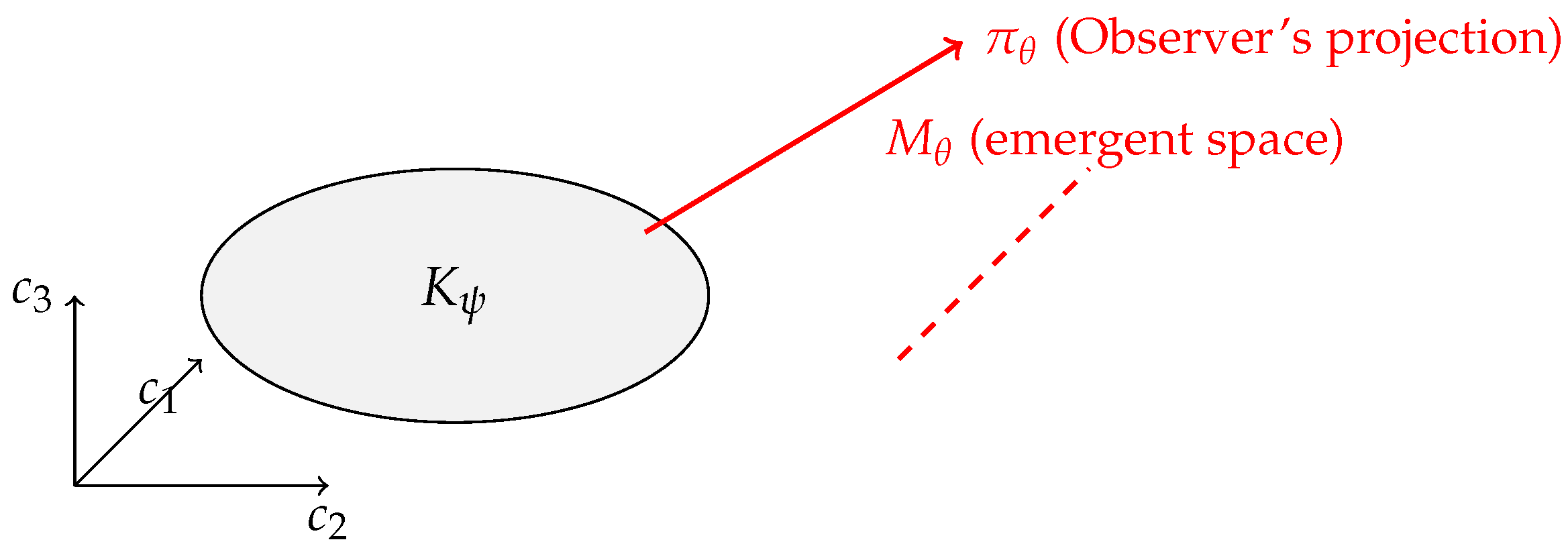
Figure 2.
Illustrative correlation density as a function of emergent separation ℓ for an entangled two-qubit state (blue) versus a separable state (red). The entangled state’s correlation density is sharply peaked at , indicating the two qubits are effectively at zero distance in the emergent space (strongly correlated in all bases). The separable state’s is broader and flatter, suggesting the qubits are far apart or disconnected in the emergent picture. The second derivative of (cf. Eq. (2) and Eq. (4)) (related to curvature) is large for the entangled case (tight peak) and nearly zero for the separable case (flat distribution), illustrating how entanglement generates curvature in the emergent geometry. Curvature is proportional to the second derivative of log .
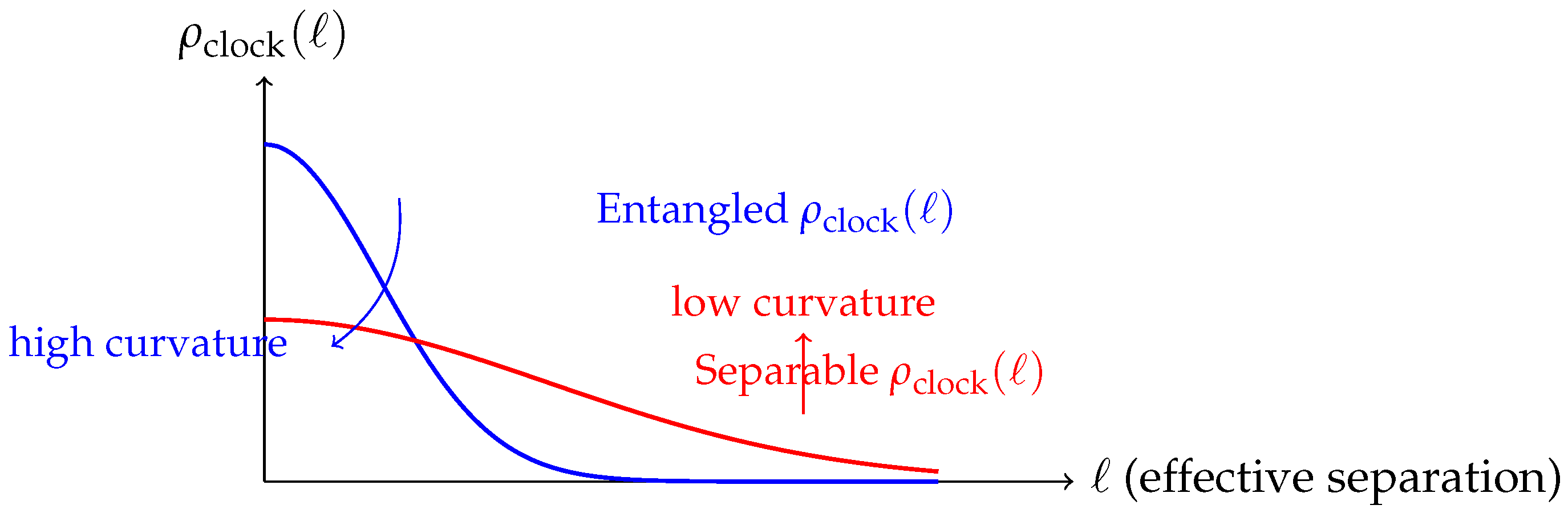
Disclaimer/Publisher’s Note: The statements, opinions and data contained in all publications are solely those of the individual author(s) and contributor(s) and not of MDPI and/or the editor(s). MDPI and/or the editor(s) disclaim responsibility for any injury to people or property resulting from any ideas, methods, instructions or products referred to in the content. |
© 2025 by the authors. Licensee MDPI, Basel, Switzerland. This article is an open access article distributed under the terms and conditions of the Creative Commons Attribution (CC BY) license (http://creativecommons.org/licenses/by/4.0/).
Copyright: This open access article is published under a Creative Commons CC BY 4.0 license, which permit the free download, distribution, and reuse, provided that the author and preprint are cited in any reuse.


