A Practical Guide to Spatial Transcriptomics: Lessons from over 1000 Samples

Eduard Porta-Pardo; Daniela Grases

doi:10.20944/preprints202504.1450.v1

Submitted:

16 April 2025

Posted:

17 April 2025

You are already at the latest version

Abstract

Spatial transcriptomics enables the in situ mapping of gene expression, revolutionizing our ability to study tissue organization and cellular interactions. However, as this technology is increasingly adopted across biological and clinical research, many groups struggle with practical barriers to implementation—including platform selection, sample quality, and experimental scalability.Here, we provide a comprehensive, practical guide to spatial transcriptomics, informed by the processing and analysis of over 1,000 spatial samples across Visium, Visium HD, and Xenium platforms. We outline best practices for experimental design, tissue handling, sequencing, and computational analysis, with special attention to clinical samples and high-throughput settings.Our goal is to translate hands-on experience into actionable recommendations that support robust, reproducible spatial workflows. This guide is designed to assist researchers at all levels—from those designing their first spatial experiment to groups aiming to integrate ST into translational pipelines and large-scale studies.

Keywords:

Spatial transcriptomics

;

visium

;

xenium

Subject:

Biology and Life Sciences - Biochemistry and Molecular Biology

Introduction

Spatial transcriptomics has rapidly transformed the way researchers explore gene expression within the context of tissue architecture[1,2,3,4]. As this technology continues to evolve at a breathtaking pace, it opens up new possibilities to understand complex cellular interactions in health and disease[5,6], as well as across organisms[7,8,9,10]. However, alongside its impressive advancements, there is a growing need for practical guidance[11] that helps scientists navigate the intricacies of the design, execution, and interpretation of spatial transcriptomics experiments.

The field of spatial transcriptomics is supported by a robust foundation of technical advancements[12,13,14,15] and rigorous benchmarking studies that have helped define key performance metrics across various platforms[16,17,18,19,20,21,22,23]. These studies have evaluated sensitivity, spatial resolution, and sequencing depth, among other technical parameters, offering a detailed snapshot of each system’s capabilities and providing key technical information that is critical in driving the field forward.

What remains missing is practical guidance: how to choose the right platform for a biological question, how to optimize sample handling and sequencing depth, and how to scale spatial experiments from pilot runs to translational pipelines involving dozens or hundreds of samples.

This guide aims to bridge that gap. Drawing from our experience processing over 1,000 spatial transcriptomics samples (Figure 1), mostly across Visium and Xenium platforms, we present a hands-on framework for designing and executing robust spatial workflows in both preclinical and clinical settings. Our recommendations are grounded in real-world scenarios: retrospective profiling of tumor samples from clinical trials, scaling up analysis pipelines for large tissue banks, and adapting protocols across tissue types and preservation methods.

While this guide draws heavily from cancer-focused applications, the principles and pitfalls we describe are broadly applicable to any lab seeking to integrate spatial transcriptomics into their research or core facility. By highlighting common challenges, critical decision points, and overlooked technical factors, we hope to support the next wave of researchers in making spatial a routine, reproducible, and scalable part of their experimental toolkit.

QuickStart: Five Lessons from 1,000+ Samples

Lesson 1: Build the right team early

Spatial transcriptomics is a multidisciplinary effort. Success depends on tight coordination between molecular biologists, pathologists, histotechnologists, and computational analysts. Involve all key players from the start.

Lesson 2: RNA quality matters, but it’s not everything

Metrics like DV200 and RIN are useful, but not definitive. We’ve recovered biologically meaningful data from below-threshold samples.

Lesson 3: Don’t skimp on sequencing

Under-sequencing is a common and costly mistake. For FFPE Visium experiments, the standard 25k reads/spot is rarely sufficient. Aim for 100k–120k reads to capture transcript diversity and support downstream analyses.

Lesson 4: Bigger gene panels can dilute your signal

With targeted imaging platforms like Xenium, more genes does not always mean better data. Larger panels often reduce per-gene sensitivity, especially for low-abundance transcripts.

Lesson 5: Batch effects are easier to prevent than to fix

Plan ahead: randomize samples, replicate where possible, and track all metadata from day one. Computational correction can help, but it’s never a full substitute for smart experimental design.

Step 1 - Defining the Research Question

The first and most critical step in any spatial transcriptomics (ST) experiment is determining whether the technology truly matches your scientific question. Not every study benefits from spatial resolution, and applying ST without a clear rationale can waste time and resources.

Begin by asking: Does the spatial organization of gene expression matter for the biological insight I’m seeking? For example, if your hypothesis involves understanding how cell–cell interactions shape the tumor microenvironment, or how specific cell states localize within a tissue, spatial context will be essential for capturing that complexity [24,25,26,27]. Conversely, if your study focuses on broad expression differences between conditions—where tissue architecture plays a minor role—bulk RNA-seq [28] or single-cell transcriptomics may be more appropriate. In addition to spatial relevance, consider the degree of cellular heterogeneity in your tissue, whether tissue structure or microanatomy is relevant, and the practical feasibility of obtaining and preserving high-quality material.

A central part of this process is deciding the spatial resolution required to answer your question. Do you need single-cell or subcellular information to study fine-grained features such as immune synapses or spatially restricted cell states? Or is a broader, spot-level overview sufficient to identify tissue-level domains, gradients, or large-scale architectural patterns [29]?

Spatial platforms span a wide range of resolutions (Figure 2), from ~55 µm (Visium), which captures multiple cells per spot, to subcellular (~2 µm) resolution in Visium-HD and imaging-based platforms such as Xenium, CosMx, and MERFISH. These high-resolution systems often offer exquisite spatial detail but typically rely on targeted gene panels. The trade-offs between resolution, gene coverage, and throughput are discussed in detail in Step 5 – Platform Selection.

You should also evaluate the required breadth of gene coverage. Discovery-driven studies may call for whole-transcriptome profiling (~18,000 genes) to identify novel markers or unexpected pathways. In contrast, hypothesis-driven questions might be addressed with mid-sized (5,000–6,000 genes) or focused (~500 genes) panels. Commercial offerings often target specific biological contexts (e.g., immuno-oncology, breast cancer), while some platforms support custom panels. For non-human species, whole-transcriptome methods are usually necessary due to limited probe availability.

Taken together, resolution, gene coverage, and platform compatibility should be viewed as interconnected decisions, grounded in the biological question. Starting with a clearly defined goal will help you avoid technical overkill—or worse, technical underperformance—and ensure your spatial transcriptomics experiment yields meaningful, interpretable insights.

Step 2 - Assemble the right team

Spatial transcriptomics is one of the most multidisciplinary workflows in molecular biology. It demands more than a solid hypothesis or a well-chosen platform—it requires a coordinated team capable of handling complex protocols, interpreting tissue morphology, and executing sophisticated data analysis.

Many ST failures are not caused by a single misstep, but from underestimating the need for early, aligned collaboration between wet lab, pathology, and computational domains (Figure 3). Involving the right people at the start is one of the most effective safeguards against wasted samples, poor data quality, or uninterpretable results.

1. Laboratory technician - Sample Preparation & Execution

Wet-lab execution is one of the most failure-prone—and often underappreciated—steps in spatial transcriptomics. These protocols are technically demanding and offer little room for recovery once errors occur. A successful experiment depends on precise sectioning, RNA-preserving workflows, and strict adherence to platform-specific protocols for permeabilization, hybridization, washing, or imaging.

Even minor deviations in section thickness, blade condition, temperature control, or reagent timing can severely impact RNA capture and spatial signal. Technicians must be comfortable not just with general molecular biology techniques, but with the specific demands of spatial workflows (e.g., Visium, Xenium, CosMx). Many platforms offer no chance to “rescue” a failed run.

Inconsistent tissue handling across samples introduces unwanted technical variation. We strongly recommend involving a dedicated spatial technician—or partnering with a specialized core facility—to ensure reproducibility. When possible, the same technician should handle all samples in a given study.

This role spans both tissue sectioning and molecular protocol execution. Sectioning requires control over thickness, orientation, and adhesion—especially for fragile, fatty, or calcified tissues (see Step 4). Importantly, the person preparing the sample must be in active communication with the broader team to align the biological question and region of interest (ROI) selection with the physical sample.

2. Pathology & Histological Input

Tissue morphology is central to interpreting spatial transcriptomics data. A trained pathologist provides critical input at multiple stages: assessing tissue quality, identifying viable and artifact-prone regions, and selecting biologically meaningful compartments such as tumor–stroma boundaries, immune infiltration zones, or anatomical landmarks.

ROIs that appear usable at low magnification may contain necrosis, fibrosis, or fixation artifacts that compromise RNA integrity or spatial interpretation. Pathologists help prevent these pitfalls, ensuring transcriptomic patterns align with biological structure rather than technical noise. In multi-sample or multi-patient studies, they also play a vital role in standardizing ROI selection, enhancing consistency and comparability across samples.

Pathologist involvement is especially important in clinical and retrospective settings, where tissue variability is high and sample quantity limited. In short: no spatial experiment should proceed without histological review. See Step 4 for detailed ROI and quality assessment strategies.

3. Bioinformatics & Data Interpretation

Spatial transcriptomics data is large, complex, and spatially structured. Bioinformaticians are essential for translating raw readouts into biological insight. Their responsibilities span multiple stages: from data preprocessing and spatial-aware normalization, to clustering, spatial domain detection, and identification of spatially variable genes.

In spot-based platforms like Visium, bioinformaticians apply deconvolution methods (e.g., RCTD, cell2location) to estimate underlying cell-type composition, while in imaging-based platforms, they manage segmentation, cell typing, and spatial modeling. They also address technical variability—such as batch effects or uneven sequencing depth—and determine when correction is necessary versus when it risks obscuring biology.

Beyond standard analysis, bioinformaticians often lead integration with other data types, including scRNA-seq, proteomics, or clinical metadata, to create a more holistic view of tissue architecture. As spatial datasets grow in scale and complexity, their role becomes even more critical for ensuring robust, reproducible interpretation. For more on computational workflows, see Step 8.

Coordination is Key

ST studies succeed when all these domains are engaged early and communicate continuously. Assigning clear responsibilities—from sectioning to interpretation—prevents downstream confusion and ensures that technical execution is aligned with biological goals. Whether in academic labs or clinical collaborations, a designated lead or coordinator helps ensure accountability, streamline decisions, and keep projects on track.

Step 3 - Experimental Design, Controls, and Statistical Power

Designing a robust spatial transcriptomics experiment requires careful planning to ensure adequate statistical power, minimize variability, and control for technical and biological confounders. Unlike bulk RNA-seq, which averages gene expression across large tissue areas, or single-cell RNA-seq, which represents an approximately random subset of the cells in a sample (unless preceded by cell sorting), spatial transcriptomics depends heavily on the precise selection of tissue sections and regions of interest. This introduces specific challenges related to sampling bias, tissue heterogeneity, and batch effects, which must be addressed through thoughtful experimental design.

A critical first step is determining how many biological replicates and ROIs are needed to detect meaningful spatial or transcriptional differences. Spatial transcriptomics experiments can be difficult to power adequately, especially when working with limited archival material[30]. In some cases, studies may analyze small tissue areas or too few samples, which limits the ability to capture intra- and inter-patient heterogeneity. To mitigate this, we recommend performing a power analysis[31,32,33,34] using pilot data to estimate the number of samples and ROIs needed to achieve statistical significance.

The choice between full tissue sections and tissue microarrays (TMAs) is another key design consideration. TMAs allow for efficient, parallel profiling of multiple samples on a single slide, reducing reagent costs and minimizing batch effects. However, the small area analyzed per sample limits detection of rare or spatially restricted features[30]. In contrast, full tissue sections provide continuous spatial context, ideal for studies of large-scale tissue architecture. Notably, reviewers often favor more biological replicates over increased spatial coverage per sample, making TMAs a useful option when working under cost or material constraints.

Batch effects can arise from differences in tissue processing, reagent batches, sequencing depth, imaging conditions, or even slide layout. These technical sources of variability can obscure biological signals if not properly addressed. To minimize batch effects, researchers should strive to standardize sample handling, randomize sample placement across slides or sequencing lanes, and process all samples under consistent conditions. Including positive and negative controls (see Box 1) further enhances interpretability and quality assurance. On the computational side, methods such as Harmony[35], Seurat[36], and Liger[37] can help align multi-sample spatial datasets, provided care is taken not to overcorrect and obscure meaningful biological variation (see Step 7).

Together, these strategies help ensure that spatial transcriptomics experiments are both technically sound and biologically interpretable—ultimately enabling confident discovery of spatial gene expression patterns and tissue organization.

Step 4 – Tissue Selection, Processing, and Quality Control

The success of spatial transcriptomics experiments depends heavily on careful tissue selection, optimal preservation, and rigorous quality control (Box 2). Variability introduced during sample handling can compromise RNA integrity, introduce technical biases, and affect data quality and interpretability. Ensuring that tissues are appropriately preserved, sectioned, and validated before proceeding to imaging detection with instrument or library preparation is therefore essential.

The first key decision is the preservation method, which may be dictated by whether the samples come from animal models or human patients. In preclinical studies, fresh-frozen tissue is often preferred due to its superior RNA integrity. However, clinical samples are typically obtained as formalin-fixed paraffin-embedded (FFPE) blocks, which are more compatible with hospital workflows and long-term storage but often contain degraded RNA due to crosslinking. Some spatial platforms, such as Visium CytAssist, Visium HD, and Xenium, now have optimized protocols for FFPE, but researchers should weigh the trade-off between tissue morphology and RNA quality based on their specific research goals.

Among the most common preservation types, fresh-frozen (FF) samples provide high RNA integrity but require ultra-low temperature storage, rapid handling, and careful cryosectioning to prevent tissue distortion from ice crystal formation. On the other hand, fixed-frozen samples allow some morphological preservation while maintaining reasonable RNA quality but are rarely used in spatial workflows. Finally, FFPE samples preserve tissue architecture well and are widely available, but the fixation process leads to RNA fragmentation. When working with FFPE blocks, we recommend storing them at 4ºC to slow further degradation.

Certain tissue types present additional challenges. Fatty tissues—such as breast, liver, or adipose-rich tumors—are notoriously difficult to section when embedded in OCT. In these cases, lowering the cryostat temperature to –30ºC and using thicker sections (>12 µm) can help produce flatter, more intact sections. FFPE-embedded fat is generally easier to cut, but care must still be taken to avoid disaggregation in the water bath; lowering the bath temperature from 42ºC to ~38ºC can help. Fatty tissues are also prone to slide detachment during processing, so we recommend using coated slides (e.g., poly-L-lysine, silane, or Superfrost Plus) and pipetting reagents slowly during the whole protocol to reduce mechanical stress. Calcified tissues—such as bone, atherosclerotic plaques, and ossified tumors—require gentle decalcification (e.g., EDTA-based methods) to improve sectioning while preserving RNA quality[38,39]. Specialized blades and low-temperature embedding can minimize fragmentation.

To reduce technical variability and improve reproducibility, we recommend standardizing section thickness whenever possible: 5 µm for FFPE tissues and 10 µm for OCT-embedded fresh-frozen samples. These dimensions have consistently produced reliable results across diverse tissue types and platforms in our experience.

Additionally, minimizing the time between sectioning and fixation or staining is critical to prevent RNA degradation, particularly for fresh-frozen samples. Prolonged exposure to room temperature—even during tissue transfer or alignment—can significantly reduce RNA quality. When working with multiple sections, organize the workflow to prioritize processing over batch cutting.

For highly heterogeneous tissues—including tumors, lymphoid organs, and developing embryos—the selection of ROIs is critical. Prior H&E staining, immunohistochemistry (IHC), DAPI staining or immunofluorescence on adjacent sections can help guide ROI selection.

RNA: RNA Quality Control

Assessing RNA integrity is a crucial step before proceeding with spatial transcriptomics. For fresh-frozen samples, a RIN (RNA Integrity Number) above 7 is generally recommended for Visium Manual protocols, though newer platforms like Visium CytAssist and Visium HD tolerate samples with RIN ≥ 4. For FFPE or fixed-frozen samples, DV200 is the more appropriate metric. This measures the percentage of RNA fragments longer than 200 nucleotides; values above 50% DV200 (Visium Manual) or 30% DV200 (Visium CytAssist and Visium HD) are typically considered acceptable. While measuring the DV200 of an FFPE block, be sure to avoid measuring fragments above 2000bp, as these often represent paraffin contamination or RNA fragments that are not likely to be amplified by the probes.

That said, in our experience, the relationship between DV200 and data quality is not perfect. For example, while Visium typically requires a DV200 ≥ 30% for optimal data quality, we have observed that data from Visium can still be informative even when DV200 is slightly lower (Figure 4). However, with platforms like Xenium, the correlation between DV200 and data quality seems somewhat stronger. This is particularly true for the Xenium Prime panel, which appears to be more sensitive to RNA degradation and may require higher DV200 values to achieve optimal data quality. In these cases, Xenium Prime may still produce robust data when samples approach the recommended DV200 threshold, but lower values can limit transcript sensitivity and gene detection. This indicates that while both platforms can handle varying levels of RNA degradation, careful consideration of DV200 and panel choice is essential to ensure the quality and reliability of the results (Figure 4).

Histological and Nuclear QC

Before beginning spatial workflows, an H&E-stained slide is indispensable for confirming tissue integrity, identifying regions of interest, and ruling out necrotic or artifact-prone areas. Hematoxylin stains nuclei blue-purple, while eosin highlights the cytoplasm and extracellular matrix in pink-red, providing a detailed view of tissue structure. This step is essential across all platforms and sample types.

For image-based methods such as Xenium and CosMx, we also recommend DAPI staining of an adjacent section to assess nuclear integrity. While DAPI is not strictly required, it can help identify unhealthy or necrotic samples before committing to high-cost assays. In our experience, good nuclear morphology correlates with improved assay success in imaging-based workflows, although it is not an absolute predictor.

Step 5 - Spatial Platform Selection

Selecting the optimal ST platform involves more than comparing technical specifications. Instead, it requires balancing scientific goals, resolution needs, sample availability, cost, and operational feasibility[40]. While several benchmarking studies and reviews have systematically compared ST technologies from a performance standpoint[16,17,18,19,20,21,22,23], here we emphasize often-overlooked practical considerations that impact experimental success (Table 1).

When Sample Quality Is a Limiting Factor

When working with low-quality FFPE or fresh-frozen samples — for example, those with DV200 < 20% or RIN < 4 — performance with whole-transcriptome platforms like Visium may be suboptimal, as degraded RNA significantly reduces transcript capture. In contrast, imaging-based platforms such as Xenium and CosMx often tolerate degraded samples better and can yield biologically meaningful data even from highly fragmented RNA. This makes them particularly attractive for archival samples or biobank material where preservation was not optimized for RNA integrity.

Whole-Transcriptome vs. Targeted Approaches

One of the most critical distinctions in spatial technologies is the scope of gene detection.

Whole-transcriptome platforms (e.g., Visium, Visium CytAssist, Visium-HD, Stereo-seq) offer broad, unbiased gene expression profiling. These are ideal for exploratory studies, identifying novel cell states, or capturing unanticipated spatial programs. However, they require high sequencing depth and often have lower spatial resolution unless using HD variants.
Targeted platforms (e.g., Xenium, CosMx, MERFISH) focus on a fixed set of genes and enable high spatial resolution, often at the single-cell or subcellular level. These approaches are well suited for hypothesis-driven studies focused on specific pathways or cell populations. The main limitation is that genes outside the panel are undetectable, limiting discovery potential.

Some platforms also support multi-modal profiling, allowing researchers to measure both RNA and proteins on the same slide. For instance, CosMx can simultaneously detect hundreds of transcripts and protein targets in a single tissue section, making it well suited for integrative phenotyping studies. Platforms like Nanostring DSP and certain MERFISH variants also enable protein co-detection, although with different limitations.

Panel Design and Sensitivity Trade-offs

In imaging-based platforms, panel size does not scale linearly with gene or transcript detection per cell. For example, when comparing the Xenium Multi-Tissue (377 genes) and Xenium Prime (5000 genes) panels, we observed that although more genes were measured in the larger panel, the median transcript count per gene dropped, indicating a trade-off between panel breadth and per-gene sensitivity (Figure 5). This nonlinear relationship suggests that larger panels dilute detection efficiency, especially for low-abundance transcripts, likely due to saturation of optical capacity or hybridization kinetics. As such, panel selection should carefully weigh the benefits of broader coverage against the loss in per-gene signal, particularly when quantitative comparisons are important.

Cross-Sample and Cross-Platform Comparability

Each platform comes with its specific biases in transcript detection, sensitivity, and resolution. Additionally, the same platform can produce divergent results depending on sample type or preservation method. For example, Visium FFPE and fresh-frozen protocols yield different transcript profiles, and datasets from these two protocols may not be directly comparable without batch correction. Similarly, while technical reproducibility within a given platform is high (especially for imaging-based technologies, Figure 5c), comparisons across panels or platforms require caution due to differences in probe design, and signal amplification.

Cost, Scalability, and Workflow Practicality

Beyond technical capabilities, real-world constraints such as cost and scalability often dictate platform choice:

Whole-transcriptome platforms typically require deeper sequencing, increasing per-sample costs and limiting scalability.
Imaging-based platforms can be more cost-effective for large-scale studies, especially when using TMAs, which allow multiple samples to be profiled on a single slide without sequencing.
Some platforms also offer higher sample multiplexing or simplified batch processing. For example, Xenium supports multiple slides per run, and CosMx allows parallel processing of RNA and protein targets, reducing the need for separate experiments.
Turnaround time is another consideration. Visium experiments can often be completed within a week (excluding sequencing), whereas CosMx and Xenium runs typically require longer, especially when imaging large tissue areas or running high-plex panels.
Workflow complexity also varies. Platforms like Visium, Visium-HD, Xenium, GeoMx and CosMx offer relatively streamlined protocols that are broadly compatible with diverse tissue types. In contrast, methods such as MERFISH or seqFISH demand specialized microscopy setups, significant user training, and often require protocol optimization for each tissue type.

Step 6 – Execution of the Experiment

Successfully executing a spatial transcriptomics experiment requires meticulous planning (Supplementary Note 1), standardized workflows, and careful real-time quality control. While platform protocols are often rigidly defined, small technical details, especially in tissue handling and reagent preparation, can be the difference between a high-quality dataset and a failed experiment. In the event of a failure during the experiment, don’t panic and contact your reagent supplier (Box 3)

Pre-experiment Setup

Before starting the experiment, it is critical to ensure that all reagents, materials, and tissues meet platform-specific quality requirements. Reagents should be freshly prepared, with strict attention to expiration dates, lot numbers, and storage conditions. Alcohols, xylene, enzymes, and buffers must be handled under recommended temperature conditions (RT, 4°C, –20°C, or –80°C, depending on the protocol). Protocol steps must be followed exactly: no improvising with microliters. Even minor deviations in reagent freshness, volumes, or incubation times can introduce inconsistencies that undermine data quality.

Tissue Sectioning and ROI Localization

Sectioning is one of the most critical and variable steps in spatial workflows. While most of the ST pipeline is highly standardized, tissue handling often allows some flexibility—and therefore introduces risk. Sectioning must be done in a RNase-free environment with clean instruments, fresh blades, and sanitized workspaces (e.g., RNase Away). Cryostats are used for OCT blocks; microtomes for FFPE.

Prior to sectioning, the ROI should be clearly identified based on an H&E or immunostained slide. In FFPE blocks, ROIs are often easier to locate due to better visibility of structures. In OCT blocks, tissue may appear pale and difficult to interpret. In such cases, we recommend a quick real-time stain of a test section to visualize key features and ensure accurate ROI selection during cryosectioning.

It is essential that the person performing the experiment understands the biological features of interest. This often requires direct communication between the person sectioning the tissue and the research team. Misalignment between what is biologically important and what is placed on the slide is a common source of failure in collaborative spatial experiments.

In both FFPE and OCT blocks, always trim 1–2 sections from the surface before collecting the section for analysis to remove tissue that has been exposed to light, RNases, or environmental contaminants. We also recommend having backup samples pre-selected for each condition, in case a sample fails at a critical stage like sectioning or placement. This allows rapid substitution without compromising experimental balance.

Handling Larger Blocks and Small ROIs

When the ROI is smaller than the full block, you can gently outline the ROI with a scalpel at the surface. During sectioning, only the marked area should be collected, separating from the rest of the section. Another option is to cut the ROI and re-embed the sample forming a new block. This method is ideal for creating tissue microarrays (TMAs), especially when placing multiple ROIs on a single slide.

Working with Tissue Microarrays (TMAs)

TMAs allow simultaneous analysis of multiple samples under identical conditions but present unique challenges1. Cores can detach during sectioning, especially those in the center, due to insufficient paraffin support. Poor alignment can also lead to core dropout, particularly near the ends of the block—studies report up to 15–33% core loss in individual slides.

Key considerations:

Core size: Larger cores (1.5–2.0 mm) are useful for preserving architecture; smaller, random cores better capture tumor heterogeneity.
Replicates and backups: Always prepare 2–3 consecutive sections in advance in case of technical failures.

Sample Preparation and Bench Practices

Once sectioning is complete, follow all protocol steps with strict attention to temperature, timing, and reagent handling:

Use RNase-free surfaces and tips
Process samples in parallel and randomized order
Control incubation time and temperature precisely
Use reagents from the same lot whenever possible
Prevent contamination by gentle pipetting and workspace cleaning
Real-time quality control should be embedded in the workflow. Monitor RNA integrity, tissue morphology, staining quality and library QC before proceeding to sequencing or imaging. These checkpoints can prevent time and resource loss on low-quality material.

Tips for Visium CytAssist Alignment

Even within rigid protocols, small tweaks can improve outcomes. For example, in the Visium CytAssist workflow, protocol recommends staining the entire tissue section with eosin (Step 4.1). However, if eosin is added only to the well without removing the slide from the cassette, it selectively stains the area that was incubated with probes. This results in a pink square (6.5 × 6.5 mm) that helps align the tissue correctly in CytAssist. Loading unstained tissue (outside the probe area) into the capture zone will produce no transcriptomic data, making alignment crucial.

Step 7 – Sequencing decisions for Spatial Transcriptomics Libraries

Sequencing is one of the most critical and costly stages of a spatial transcriptomics experiment. It often represents the final opportunity to impact data quality before analysis begins. While most protocols recommend sequencing to approximately 50-70% saturation, our experience has shown that this is frequently insufficient to recover the full biological potential of the samples, especially when dealing with heterogeneous tissues. In practice, deeper sequencing can substantially improve sensitivity, and enable more robust downstream analyses such as cell type deconvolution, pathway scoring, or spatial domain identification.

Coverage saturation refers to the proportion of reads that contribute new information—specifically, reads with unique combinations of spatial barcode, UMI, and gene identity. As saturation increases, each additional read is increasingly likely to duplicate information already captured. For example, a sample with 50% saturation is still gaining new UMIs from half of the sequencing reads, whereas one at 85% saturation is largely saturated in terms of information yield. However, saturation is not an absolute indicator of quality. A sample can reach 50% saturation and still exhibit low transcript or gene detection if the RNA quality is poor, or if sequencing reads are consumed disproportionately by a few highly expressed genes. This makes it essential to consider saturation alongside metrics such as median genes per spot or per cell, total UMIs, and spatial coverage uniformity (Figure 6).

When planning a spatial experiment, we strongly advise allocating enough budget for high-quality sequencing. Under-sequencing can waste an otherwise successful experiment. In our experience, sequencing beyond vendor-recommended minimums can substantially improve data utility. For instance, in Visium HD experiments, we routinely aim for around 700 million read pairs per sample when working with a 6 × 6 mm tissue area. This depth allows reliable transcript detection across diverse cell types, including low-abundance populations, and enables more confident interpretation of subtle spatial patterns. Achieving this depth typically limits us to two-three samples per NovaSeq X lane, illustrating how spatial experiments can become sequencing-limited and why realistic budgeting is essential from the beginning.

While it may be tempting to multiplex more samples per run to save costs, doing so without careful consideration of tissue area and RNA integrity can result in uneven coverage and variable data quality. Not all samples require the same number of reads—those with larger tissue sections or higher RNA quality will consume a larger share of sequencing bandwidth. Consequently, it’s important to balance samples appropriately across lanes and anticipate variable performance.

Ultimately, sequencing is where experimental precision meets financial constraint. Cutting corners at this stage risks compromising the entire dataset. When planning a spatial transcriptomics study—especially one with limited sample availability or one where biological replicates are precious—it is better to sequence fewer samples well than more samples poorly. A carefully designed sequencing strategy ensures that the biological insights generated by spatial technologies are not lost to technical undersampling.

Step 8 – Data Processing, Normalization, and Interpretation

Spatial transcriptomics datasets are rich, complex, and unlike traditional RNA-seq—they capture gene expression alongside physical location, introducing new opportunities for insight, but also new layers of complexity.

The goal of spatial analysis is not just to identify genes that are differentially expressed, but to understand how those genes are spatially distributed, how they define tissue architecture, and how they reflect cellular interactions in situ. This requires a workflow that integrates quality control, normalization, dimensionality reduction, and spatial modeling—while accounting for the quirks of each platform [41,42].

Robust metadata collection is essential for reproducibility, interoperability, and large-scale integration of spatial transcriptomics data. This includes not only technical parameters—such as platform, protocol version, tissue section orientation, RNA quality metrics, and sequencing depth—but also biological metadata, including patient characteristics, disease stage, anatomical location, treatment status, and histopathological features. Without standardized metadata, it becomes difficult to compare datasets across studies or interpret spatial findings in clinical and biological context. Initiatives like the Human Tumor Atlas Network[43] (HTAN) and HuBMAP[44] emphasize the importance of comprehensive, structured metadata schemas to ensure data utility and adherence to FAIR (Findable, Accessible, Interoperable, and Reusable) principles.

Quality control and normalization steps for spatial transcriptomics are similar across sequencing-based approaches and imaging-based methods, differing mainly in whether filtering is applied at the spot or cell level. Quality control involves removing low-quality data points—spots with insufficient transcript counts or cells with minimal gene expression. Genes expressed in only a small fraction of spots or cells may also be eliminated to ensure robust downstream analysis. Normalization strategies such as log normalization or SCTransform then addresses variations in sequencing depth or signal intensity, which can vary greatly across spots or cells, and is crucial for generating reliable biological insights in subsequent analyses[45].

A key next step in spatial transcriptomics is extracting meaningful insights via dimensionality reduction, clustering, and spatially variable gene (SVG) analysis[41]. It is equally important to distinguish true biological variation—such as tissue architecture, cell–cell interactions, and microenvironmental influences—from technical noise introduced by varying sequencing depths, uneven tissue sectioning, or platform-specific biases. Orthogonal validation methods (e.g., immunohistochemistry, spatial proteomics, multiplex imaging) offer independent confirmation of transcriptomic signals, helping researchers ensure that observed spatial patterns are not merely artifacts.

For multi-sample or cross-platform studies, batch correction (e.g., Harmony, Seurat, or Liger) can reduce technical variability without obscuring meaningful tissue-specific signals, though overcorrection should be avoided. Where batch effects are minimal, correction may not be necessary. Integrating ST data with single-cell RNA-seq (scRNA-seq) further clarifies cell type composition—particularly for spot-level platforms (e.g., 10x Visium) where tools such as RCTD[46] or cell2location[47] deconvolve mixed signals. Bulk RNA-seq can provide a complementary overview, while spatial proteomics and multiplex imaging correlate mRNA levels with protein expression for an additional layer of validation.

Gene imputation approaches (e.g., Tangram) help address dropout by inferring the locations of lowly expressed genes. Neighboring cells or spots, however, often display correlated expression profiles—a phenomenon known as “spatial autocorrelation”. Because most classical statistical tests assume data points are independent, overlooking this correlation can inflate false positives or hide genuine effects. Local statistics such as Moran’s I or Geary’s C help reveal whether observed clusters are biologically meaningful rather than random artifacts[42]. Visualization through spatial heatmaps, 3D tissue mapping, or overlays of gene expression onto histological features further enhances interpretability.

Given the diversity and rapid development of computational tools in spatial transcriptomics, systematic benchmarking of analysis methods is increasingly important. Current workflows vary widely in performance depending on tissue type, resolution, and data quality. Dedicated efforts are now emerging to evaluate algorithms for quality control[48], clustering and spatial gene detection[49,50,51,52,53], and deconvolution[54,55], helping establish best practices. These benchmarks not only guide tool selection but also promote reproducibility and interoperability across studies and platforms.

Finally, spot-based platforms (e.g., 10x Visium) enable comprehensive, whole-transcriptome profiling that lends itself to broad gene expression and (meta)pathway-level analyses[29]. By contrast, imaging-based methods (e.g. 10x Xenium) are inherently cell-resolved but often rely on more cost-efficient, limited gene panels (e.g., hundreds to a few thousand genes). While this smaller panel size may be sufficient to precisely identify and segment specific cell types for neighborhood or community-level research[24], it can be less ideal for genome-wide or pathway-focused investigations. Each approach thus provides unique strengths—spot-level platforms for unbiased global discovery and imaging-based systems for high-resolution, cell-level insights. Emerging technologies such as Visium HD bridge these advantages by offering single-cell resolution alongside near whole transcriptome coverage, promising a more unified view of tissue complexity.

Future Directions: AI, Multi-Omics, and Clinical Applications

Spatial transcriptomics is rapidly evolving, with new platforms pushing resolution toward single-cell and even subcellular scales. These advances are enabling finer dissection of cell–cell interactions, tumor microenvironments, and tissue remodeling, while preserving morphological context, even in 3D [56,57,58]. In parallel, multi-omics approaches are extending beyond transcriptomics to include proteomics, epigenomics, and metabolomics, offering increasingly comprehensive molecular maps of intact tissues.

Artificial intelligence is poised to accelerate spatial data interpretation[59,60,61]. Deep learning models and graph-based neural networks can enhance cell type annotation, infer tissue architecture, and detect subtle spatial features that may be predictive of clinical outcomes. These tools will be critical for scaling spatial analyses, particularly as dataset size and complexity increase.

Clinical integration is on the horizon[62]. In oncology, spatial transcriptomics is already being explored to identify resistance niches, stratify patients by microenvironmental signatures, and refine biomarker development. Prospective trials and retrospective cohort analyses are beginning to demonstrate how spatial profiling can complement histopathology and traditional genomics in guiding treatment decisions.

Initiatives like the HTAN[43] are setting new standards for interoperability, multimodal integration, and cross-study reproducibility. These efforts, along with improvements in automation and cost reduction, will be essential for making spatial technologies broadly accessible—not just in research, but in diagnostics and precision medicine.

Spatial at Scale: From Feasibility to Impact

While spatial transcriptomics is rapidly evolving, its adoption at scale remains a challenge for many research groups. Over the past four years, our lab has implemented spatial workflows across more than 1,000 samples—ranging from prospective mouse studies to complex retrospective human tumor cohorts—using platforms such as Visium and Xenium. These efforts have included multiple cancer types, tissue formats (FFPE and fresh-frozen), and clinical contexts, including retrospective analysis of samples from neoadjuvant trials.

Scaling spatial experiments from pilot to cohort-level studies required more than protocol adherence. It demanded standardized wet-lab practices, coordination between computational and experimental teams, robust quality control checkpoints, and proactive engagement with collaborators—particularly in clinical and pathology settings. Decisions about tissue selection, platform choice, sequencing depth, and metadata capture had to be embedded into a reproducible framework that could support high-throughput workflows without compromising data quality or interpretability.

One of the most important insights from this experience is that scaling spatial transcriptomics is not only possible, but essential for translational research. Single-sample experiments rarely capture the heterogeneity required to uncover robust spatial biomarkers, while large-scale datasets offer new opportunities to link spatial architecture to treatment response, clonal dynamics, and patient outcomes. This scaling process is not purely technical; it is organizational, logistical, and scientific.

We hope this guide empowers other teams—whether in academic labs, core facilities, or clinical research units—to move beyond proof-of-concept and toward routine, reliable spatial transcriptomics at scale. As the field matures, it will not be the most advanced technology alone that drives impact, but the ability to deploy spatial approaches systematically, reproducibly, and in direct service of biological and clinical insight.

Acknowledgements

We would like to thank the Josep Carreras Leukaemia Research Institute, and Manel Esteller in particular, for their incredible support for spatial transcriptomics projects at our institute over the last 4 years, which has made this guide possible. We also would like to thank all our collaborators for their confidence in us, and Sergi Cervilla, Mustafa Sibai, and Amanda Garza for their feedback and discussion about the manuscript. E.P-P. is supported by by the Spanish Ministry of Science (RYC2019-026415-I MICIU/AEI/10.13039/501100011033, "El FSE invierte en tu futuro"), Fundación FERO-ASEICA (BFERO2002.6), and Generalitat de Catalunya (SGR007). E.P-P. and D.G. are supported by Fundació Josep Carreras Contra la Leucemia. IJC is supported by MCIU as a Centro de Excelencia Severo Ochoa (CEX2023- 001258-S, MCIN/AEI/10.13039/501100011033).

References

Williams, C.G.; Lee, H.J.; Asatsuma, T.; Vento-Tormo, R.; Haque, A. An introduction to spatial transcriptomics for biomedical research. Genome Med. 2022, 14, 68. [Google Scholar] [CrossRef] [PubMed]
Rao, A.; Barkley, D.; França, G.S.; Yanai, I. Exploring tissue architecture using spatial transcriptomics. Nature 2021, 596, 211–220. [Google Scholar] [CrossRef]
Bressan, D.; Battistoni, G.; Hannon, G.J. The dawn of spatial omics. Science 2023, 381, eabq4964. [Google Scholar] [CrossRef]
Marx, V. Method of the Year: spatially resolved transcriptomics. Nat. Methods 2021, 18, 9–14. [Google Scholar] [CrossRef]
Jin, Y.; Zuo, Y.; Li, G.; Liu, W.; Pan, Y.; Fan, T.; Fu, X.; Yao, X.; Peng, Y. Advances in spatial transcriptomics and its applications in cancer research. Mol. Cancer 2024, 23, 129. [Google Scholar] [CrossRef] [PubMed]
Fomitcheva-Khartchenko, A.; Kashyap, A.; Geiger, T.; Kaigala, G.V. Space in cancer biology: its role and implications. Trends Cancer 2022, 8, 1019–1032. [Google Scholar] [CrossRef]
Saarenpää, S.; Shalev, O.; Ashkenazy, H.; Carlos, V.; Lundberg, D.S.; Weigel, D.; et al. Spatial metatranscriptomics resolves host-bacteria-fungi interactomes. Nat Biotechnol. 2024, 42, 1384–1393. [Google Scholar] [CrossRef]
Fu, Y.; Xiao, W.; Tian, L.; Guo, L.; Ma, G.; Ji, C.; Huang, Y.; Wang, H.; Wu, X.; Yang, T.; et al. Spatial transcriptomics uncover sucrose post-phloem transport during maize kernel development. Nat. Commun. 2023, 14, 7191. [Google Scholar] [CrossRef]
Song, X.; Guo, P.; Xia, K.; Wang, M.; Liu, Y.; Chen, L.; Zhang, J.; Xu, M.; Liu, N.; Yue, Z.; et al. Spatial transcriptomics reveals light-induced chlorenchyma cells involved in promoting shoot regeneration in tomato callus. Proc. Natl. Acad. Sci. USA 2023, 120, e2310163120. [Google Scholar] [CrossRef]
Johnson, Z.V.; Hegarty, B.E.; Gruenhagen, G.W.; Lancaster, T.J.; McGrath, P.T.; Streelman, J.T. Cellular profiling of a recently-evolved social behavior in cichlid fishes. Nat. Commun. 2023, 14, 4891. [Google Scholar] [CrossRef]
Valihrach, L.; Zucha, D.; Abaffy, P.; Kubista, M. A practical guide to spatial transcriptomics. Mol. Asp. Med. 2024, 97, 101276. [Google Scholar] [CrossRef] [PubMed]
Ren, J.; Luo, S.; Shi, H.; Wang, X. Spatial omics advances for in situ RNA biology. Mol. Cell 2024, 84, 3737–3757. [Google Scholar] [CrossRef] [PubMed]
Moffitt, J.R.; Lundberg, E.; Heyn, H. The emerging landscape of spatial profiling technologies. Nat Rev Genet. 2022, 23, 741–759. [Google Scholar] [CrossRef]
Tian, L.; Chen, F.; Macosko, E.Z. The expanding vistas of spatial transcriptomics. Nat. Biotechnol. 2022, 41, 773–782. [Google Scholar] [CrossRef] [PubMed]
Moses, L.; Pachter, L. Museum of spatial transcriptomics. Nat Methods 2022, 19, 534–546. [Google Scholar] [CrossRef]
Cook, D.P.; Jensen, K.B.; Wise, K.; Roach, M.J.; Dezem, F.S.; Ryan, N.K.; et al. A comparative analysis of imaging-based spatial transcriptomics platforms. bioRxiv 2023. [Google Scholar] [CrossRef]
Wang, T.; Harvey, K.; Reeves, J.; Roden, D.L.; Bartonicek, N.; Yang, J.; et al. An experimental comparison of the Digital Spatial Profiling and Visium spatial transcriptomics technologies for cancer research. bioRxiv 2023. [Google Scholar] [CrossRef]
Ren, P.; Zhang, R.; Wang, Y.; Zhang, P.; Luo, C.; Wang, S.; et al. Systematic benchmarking of high-throughput subcellular spatial transcriptomics platforms. bioRxiv 2024. [Google Scholar] [CrossRef]
Wang, H.; Huang, R.; Nelson, J.; Gao, C.; Tran, M.; Yeaton, A.; et al. Systematic benchmarking of imaging spatial transcriptomics platforms in FFPE tissues. bioRxiv 2023. [Google Scholar] [CrossRef]
You, Y.; Fu, Y.; Li, L.; Zhang, Z.; Jia, S.; Lu, S.; Ren, W.; Liu, Y.; Xu, Y.; Liu, X.; et al. Systematic comparison of sequencing-based spatial transcriptomic methods. Nat. Methods 2024, 21, 1743–1754. [Google Scholar] [CrossRef]
Rademacher, A.; Huseynov, A.; Bortolomeazzi, M.; Wille, S.J.; Schumacher, S.; Sant, P.; et al. Comparison of spatial transcriptomics technologies using tumor cryosections. bioRxiv 2024. [Google Scholar] [CrossRef]
Cervilla, S.; Grases, D.; Perez, E.; Real, F.X.; Musulen, E.; Esteller, M.; et al. Comparison of spatial transcriptomics technologies across six cancer types. bioRxiv 2024. [Google Scholar] [CrossRef]
Du, M.R.M.; Wang, C.; Law, C.W.; Amann-Zalcenstein, D.; Anttila, C.J.A.; Ling, L.; Hickey, P.F.; Sargeant, C.J.; Chen, Y.; Ioannidis, L.J.; et al. Benchmarking spatial transcriptomics technologies with the multi-sample SpatialBenchVisium dataset. Genome Biol. 2025, 26, 77. [Google Scholar] [CrossRef]
Grande, E.; Sibai, M.; Andrada, E.; Grases, D.; Reig, O.; Escobosa, M.; et al. Spatial biomarkers of response to neoadjuvant therapy in muscle-invasive bladder cancer: the DUTRENEO trial. medRxiv 2025. [Google Scholar] [CrossRef]
Arnol, D.; Schapiro, D.; Bodenmiller, B.; Saez-Rodriguez, J.; Stegle, O. Modeling Cell-Cell Interactions from Spatial Molecular Data with Spatial Variance Component Analysis. Cell Rep. 2019, 29, 202–211e6. [Google Scholar] [CrossRef] [PubMed]
Pham, D.; Tan, X.; Balderson, B.; Xu, J.; Grice, L.F.; Yoon, S.; Willis, E.F.; Tran, M.; Lam, P.Y.; Raghubar, A.; et al. Robust mapping of spatiotemporal trajectories and cell–cell interactions in healthy and diseased tissues. Nat. Commun. 2023, 14, 7739. [Google Scholar] [CrossRef]
Ferri-Borgogno, S.; Zhu, Y.; Sheng, J.; Burks, J.K.; Gomez, J.A.; Wong, K.K.; Wong, S.T.; Mok, S.C. Spatial Transcriptomics Depict Ligand–Receptor Cross-talk Heterogeneity at the Tumor-Stroma Interface in Long-Term Ovarian Cancer Survivors. Cancer Res. 2023, 83, 1503–1516. [Google Scholar] [CrossRef]
Li, Y.; Porta-Pardo, E.; Tokheim, C.; Bailey, M.H.; Yaron, T.M.; Stathias, V.; Geffen, Y.; Imbach, K.J.; Cao, S.; Anand, S.; et al. Pan-cancer proteogenomics connects oncogenic drivers to functional states. Cell 2023, 186, 3921–3944.e25. [Google Scholar] [CrossRef]
Sibai, M.; Cervilla, S.; Grases, D.; Musulen, E.; Lazcano, R.; Mo, C.-K.; Davalos, V.; Fortian, A.; Bernat, A.; Romeo, M.; et al. The spatial landscape of cancer hallmarks reveals patterns of tumor ecological dynamics and drug sensitivity. Cell Rep. 2025, 44, 115229. [Google Scholar] [CrossRef]
Lin, J.-R.; Wang, S.; Coy, S.; Chen, Y.-A.; Yapp, C.; Tyler, M.; Nariya, M.K.; Heiser, C.N.; Lau, K.S.; Santagata, S.; et al. Multiplexed 3D atlas of state transitions and immune interaction in colorectal cancer. Cell 2023, 186, 363–381.e19. [Google Scholar] [CrossRef]
Bost, P.; Schulz, D.; Engler, S.; Wasserfall, C.; Bodenmiller, B. Optimizing multiplexed imaging experimental design through tissue spatial segregation estimation. Nat. Methods 2022, 20, 418–423. [Google Scholar] [CrossRef] [PubMed]
Baker, E.A.G.; Schapiro, D.; Dumitrascu, B.; Vickovic, S.; Regev, A. In silico tissue generation and power analysis for spatial omics. Nat. Methods 2023, 20, 424–431. [Google Scholar] [CrossRef]
Shui, L.; Maitra, A.; Yuan, Y.; Lau, K.; Kaur, H.; Li, L.; et al. PoweREST: Statistical Power Estimation for Spatial Transcriptomics Experiments to Detect Differentially Expressed Genes Between Two Conditions. bioRxiv 2024. [Google Scholar] [CrossRef]
Xie, J.; Jeon, H.; Chang, W.; Jeon, Y.; Li, Z.; Ma, Q.; et al. SpaDesign: A statistical framework to improve the design of sequencing-based spatial transcriptomics experiments. bioRxiv 2024. [Google Scholar] [CrossRef]
Korsunsky, I.; Millard, N.; Fan, J.; Slowikowski, K.; Zhang, F.; Wei, K.; Baglaenko, Y.; Brenner, M.; Loh, P.-R.; Raychaudhuri, S. Fast, sensitive and accurate integration of single-cell data with Harmony. Nat. Methods 2019, 16, 1289–1296. [Google Scholar] [CrossRef] [PubMed]
Hao, Y.; Stuart, T.; Kowalski, M.H.; Choudhary, S.; Hoffman, P.; Hartman, A.; Srivastava, A.; Molla, G.; Madad, S.; Fernandez-Granda, C.; et al. Dictionary learning for integrative, multimodal and scalable single-cell analysis. Nat. Biotechnol. 2023, 42, 293–304. [Google Scholar] [CrossRef]
Welch, J.D.; Kozareva, V.; Ferreira, A.; Vanderburg, C.; Martin, C.; Macosko, E.Z. Single-Cell Multi-omic Integration Compares and Contrasts Features of Brain Cell Identity. Cell 2019, 177, 1873–1887.e17. [Google Scholar] [CrossRef]
Cooper, R.A.; Thomas, E.; Sozanska, A.M.; Pescia, C.; Royston, D.J. Spatial transcriptomic approaches for characterising the bone marrow landscape: pitfalls and potential. Leukemia 2024, 39, 291–295. [Google Scholar] [CrossRef]
Yip, R.K.; Hawkins, E.D.; Bowden, R.; Rogers, K.L. Towards deciphering the bone marrow microenvironment with spatial multi-omics. Semin. Cell Dev. Biol. 2025, 167, 10–21. [Google Scholar] [CrossRef]
Lim, H.J.; Wang, Y.; Buzdin, A.; Li, X. A practical guide for choosing an optimal spatial transcriptomics technology from seven major commercially available options. BMC Genom. 2025, 26, 47. [Google Scholar] [CrossRef]
Dries, R.; Chen, J.; del Rossi, N.; Khan, M.M.; Sistig, A.; Yuan, G.-C. Advances in spatial transcriptomic data analysis. Genome Res. 2021, 31, 1706–1718. [Google Scholar] [CrossRef] [PubMed]
Zormpas, E.; Queen, R.; Comber, A.; Cockell, S.J. Mapping the transcriptome: Realizing the full potential of spatial data analysis. Cell 2023, 186, 5677–5689. [Google Scholar] [CrossRef]
Rozenblatt-Rosen, O.; Regev, A.; Oberdoerffer, P.; Nawy, T.; Hupalowska, A.; Rood, J.E.; Ashenberg, O.; Cerami, E.; Coffey, R.J.; Demir, E.; et al. The Human Tumor Atlas Network: Charting Tumor Transitions across Space and Time at Single-Cell Resolution. Cell 2020, 181, 236–249. [Google Scholar] [CrossRef]
Hu, B.C. The human body at cellular resolution: the NIH Human Biomolecular Atlas Program. Nature 2019, 574, 187–192. [Google Scholar] [CrossRef]
Stuart, T.; Butler, A.; Hoffman, P.; Hafemeister, C.; Papalexi, E.; Mauck WM3rd et, a.l. Comprehensive Integration of Single-Cell Data. Cell 2019, 177, 1888–1902e21. [Google Scholar] [CrossRef] [PubMed]
Cable, D.M.; Murray, E.; Zou, L.S.; Goeva, A.; Macosko, E.Z.; Chen, F.; Irizarry, R.A. Robust decomposition of cell type mixtures in spatial transcriptomics. Nat. Biotechnol. 2021, 40, 517–526. [Google Scholar] [CrossRef]
Kleshchevnikov, V.; Shmatko, A.; Dann, E.; Aivazidis, A.; King, H.W.; Li, T.; Elmentaite, R.; Lomakin, A.; Kedlian, V.; Gayoso, A.; et al. Cell2location maps fine-grained cell types in spatial transcriptomics. Nat. Biotechnol. 2022, 40, 661–671. [Google Scholar] [CrossRef]
Liang, X.; Torkel, M.; Cao, Y.; Yang, J.Y.H. Multi-task benchmarking of spatially resolved gene expression simulation models. Genome Biol. 2025, 26, 1–26. [Google Scholar] [CrossRef] [PubMed]
Charitakis, N.; Salim, A.; Piers, A.T.; Watt, K.I.; Porrello, E.R.; Elliott, D.A.; Ramialison, M. Disparities in spatially variable gene calling highlight the need for benchmarking spatial transcriptomics methods. Genome Biol. 2023, 24, 209. [Google Scholar] [CrossRef]
Chen, X.; Ran, Q.; Tang, J.; Chen, Z.; Huang, S.; Shi, X.; Xi, R. Benchmarking algorithms for spatially variable gene identification in spatial transcriptomics. Bioinformatics 2025. Online ahead of print. [Google Scholar] [CrossRef]
Yuan, Z.; Zhao, F.; Lin, S.; Zhao, Y.; Yao, J.; Cui, Y.; Zhang, X.-Y.; Zhao, Y. Benchmarking spatial clustering methods with spatially resolved transcriptomics data. Nat. Methods 2024, 21, 712–722. [Google Scholar] [CrossRef] [PubMed]
Chen, C.; Kim, H.J.; Yang, P. Evaluating spatially variable gene detection methods for spatial transcriptomics data. Genome Biol. 2024, 25, 18. [Google Scholar] [CrossRef] [PubMed]
Reynoso, S.; Schiebout, C.; Krishna, R.; Zhang, F. STEAM: Spatial Transcriptomics Evaluation Algorithm and Metric for clustering performance. bioRxiv 2025. [Google Scholar] [CrossRef]
Chen, J.; Liu, W.; Luo, T.; Yu, Z.; Jiang, M.; Wen, J.; Gupta, G.P.; Giusti, P.; Zhu, H.; Yang, Y.; et al. A comprehensive comparison on cell-type composition inference for spatial transcriptomics data. Briefings Bioinform. 2022, 23. [Google Scholar] [CrossRef]
Cheng, J.; Jin, X.; Smyth, G.K.; Chen, Y. Benchmarking cell type annotation methods for 10x Xenium spatial transcriptomics data. BMC Bioinform. 2025, 26, 22. [Google Scholar] [CrossRef]
Mo, C.-K.; Liu, J.; Chen, S.; Storrs, E.; da Costa, A.L.N.T.; Houston, A.; Wendl, M.C.; Jayasinghe, R.G.; Iglesia, M.D.; Ma, C.; et al. Tumour evolution and microenvironment interactions in 2D and 3D space. Nature 2024, 634, 1178–1186. [Google Scholar] [CrossRef] [PubMed]
Bouwman, B.A.; Crosetto, N.; Bienko, M. The era of 3D and spatial genomics. Trends Genet. 2022, 38, 1062–1075. [Google Scholar] [CrossRef]
Schott, M.; León-Periñán, D.; Splendiani, E.; Strenger, L.; Licha, J.R.; Pentimalli, T.M.; Schallenberg, S.; Alles, J.; Tagliaferro, S.S.; Boltengagen, A.; et al. Open-ST: High-resolution spatial transcriptomics in 3D. Cell 2024, 187, 3953–3972.e26. [Google Scholar] [CrossRef] [PubMed]
Luo, J.; Fu, J.; Lu, Z.; Tu, J. Deep learning in integrating spatial transcriptomics with other modalities. Briefings Bioinform. 2024, 26. [Google Scholar] [CrossRef]
Wang, C.; Cui, H.; Zhang, A.; Xie, R.; Goodarzi, H.; Wang, B. ScGPT-spatial: Continual pretraining of single-cell foundation model for spatial transcriptomics. bioRxiv 2025. [Google Scholar] [CrossRef]
Wang, H.; He, Y.; Coelho, P.P.; Bucci, M.; Nazir, A.; Chen, B.; et al. SpatialAgent: An Autonomous AI Agent for Spatial Biology. bioRxiv 2025. [Google Scholar] [CrossRef]
Chen, J.; Larsson, L.; Swarbrick, A.; Lundeberg, J. Spatial landscapes of cancers: insights and opportunities. Nat. Rev. Clin. Oncol. 2024, 21, 660–674. [Google Scholar] [CrossRef] [PubMed]

Notes

1.	https://kb.10xgenomics.com/hc/en-us/articles/14612373280269-Do-you-have-recommendations-for-sectioning-TMAs-for-Xenium

Figure 1. Our experience with spatial transcriptomics. a) Number of samples processed at our laboratory over the last five years depending on the spatial transcriptomics platform. Not all processed samples have been included in this plot due to confidentiality issues. b) Fraction of samples according to whether they are cancer-related or not (left), the type of embedding (middle), and the species (right).

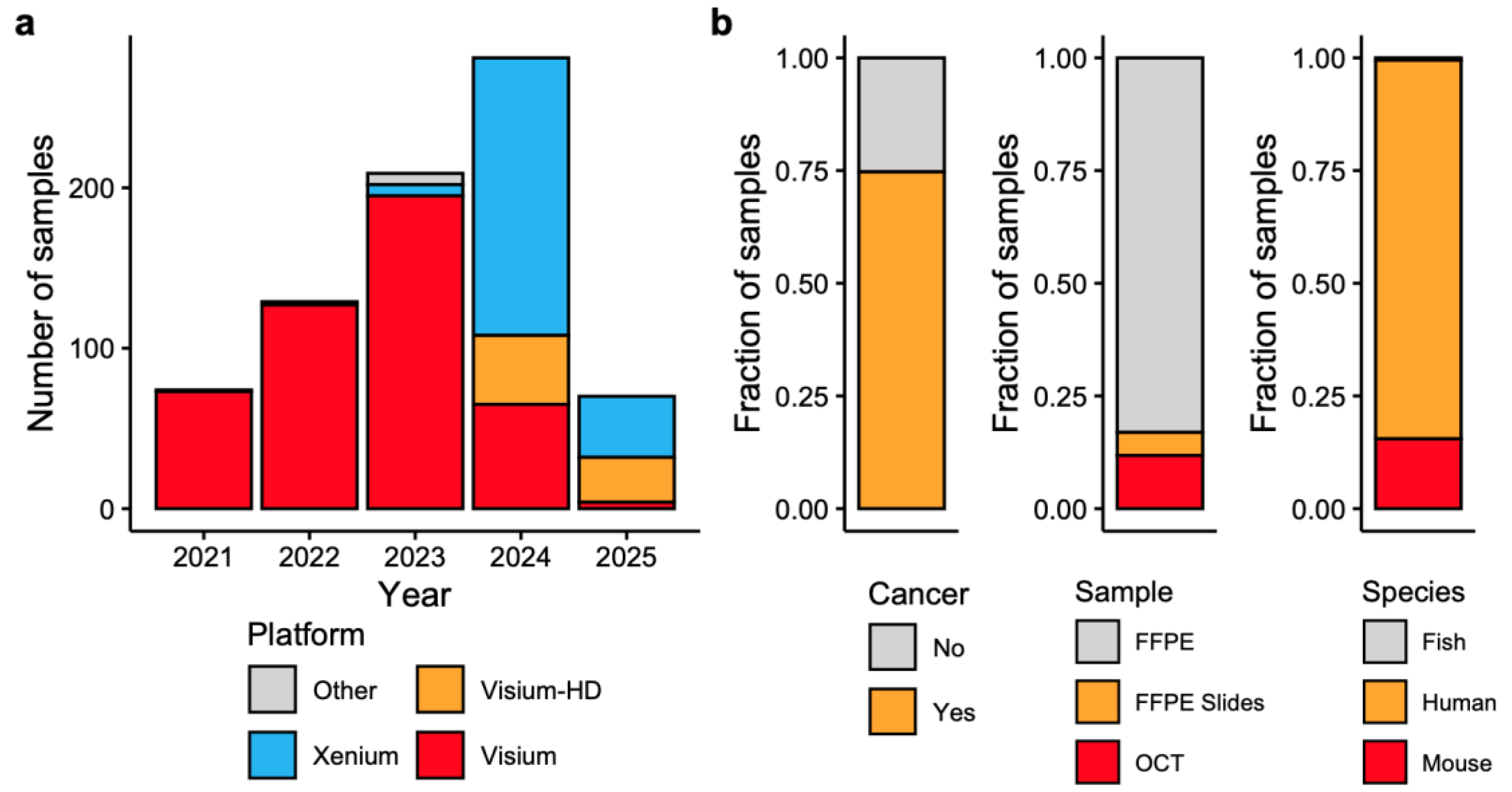
Figure 2. Differences in resolution between ST platforms. a) An H&E image of an ovarian tumor. b) The same tumor area with cells segmented and colored according to the cell type annotated from Xenium data. c) Overlay of the Visium spots (55µm) in the same area, showing the oligo-cell resolution of this platform. d) Zoom into one of the spots from “c” with an overlay of the Visium-HD grid (2µm), showing the sub-cellular resolution of this platform.

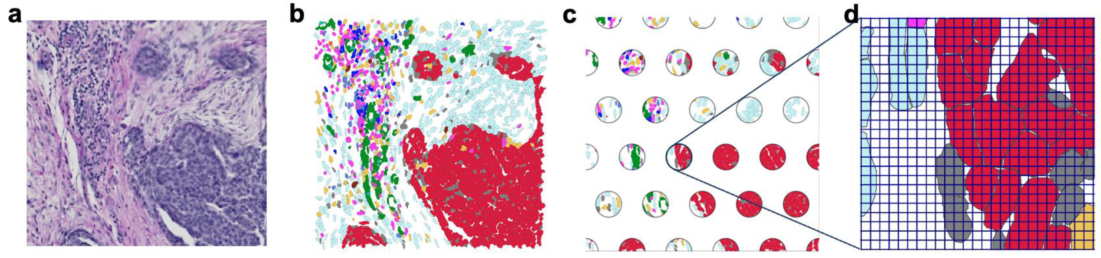
Figure 3. Assembling the right team. The success of spatial transcriptomics projects critically depends on having the right team involved across all stages. Before beginning the project, be sure to have people with experience in all the following: molecular biology, computational biology, and pathology. Missing any of these key components will likely result in failed projects and wasted resources.

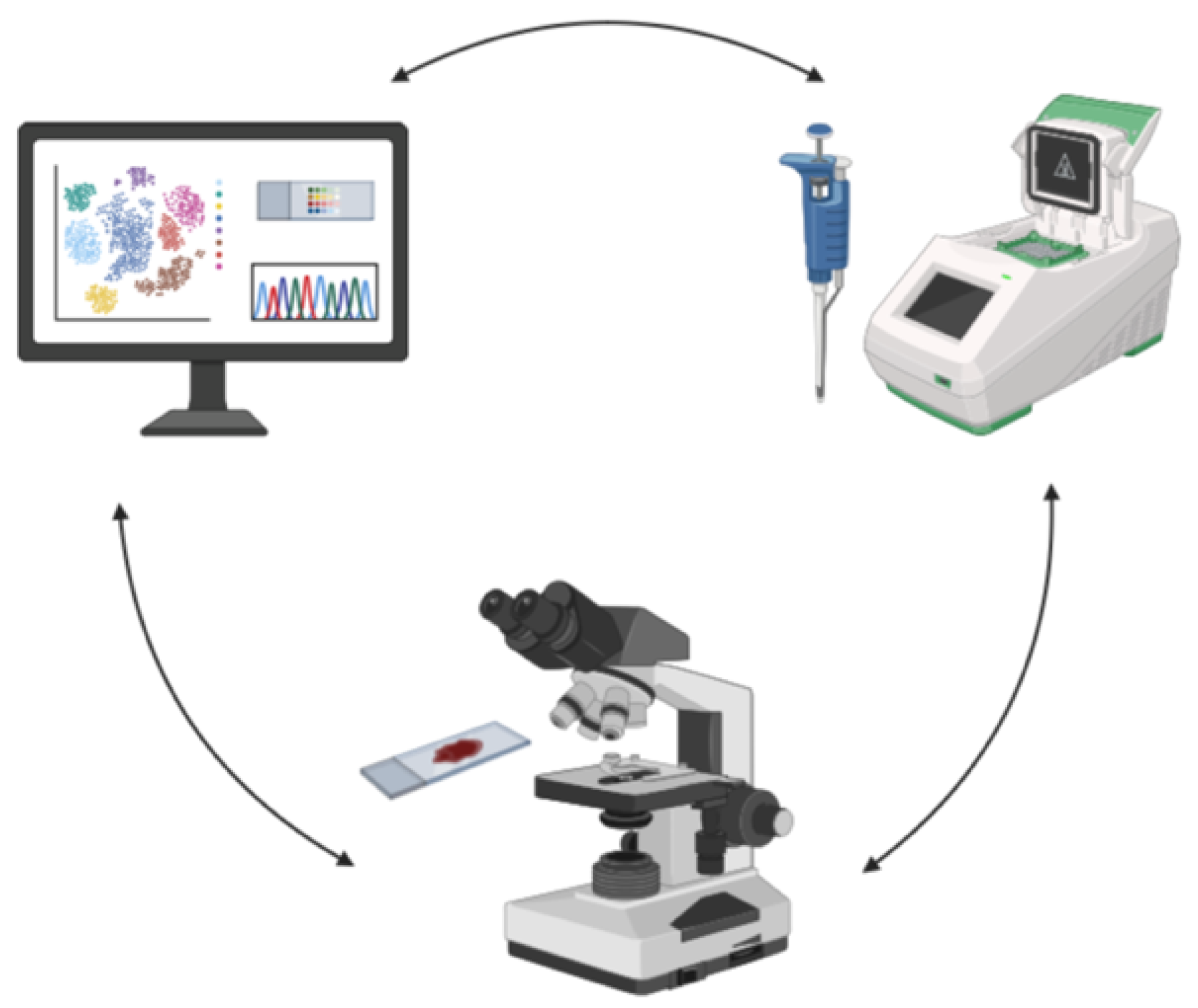
Figure 4. Relationship between DV200 and data quality. a) Correlation between DV200 of the FFPE block (x-axis) and the median genes per spot obtained in Visium (y-axis) across 137 tumor samples. b) Correlation between the DV200 of the FFPE block (x-axis) and the median transcripts per cell (y-axis) obtained with Xenium depending on the gene panel used.

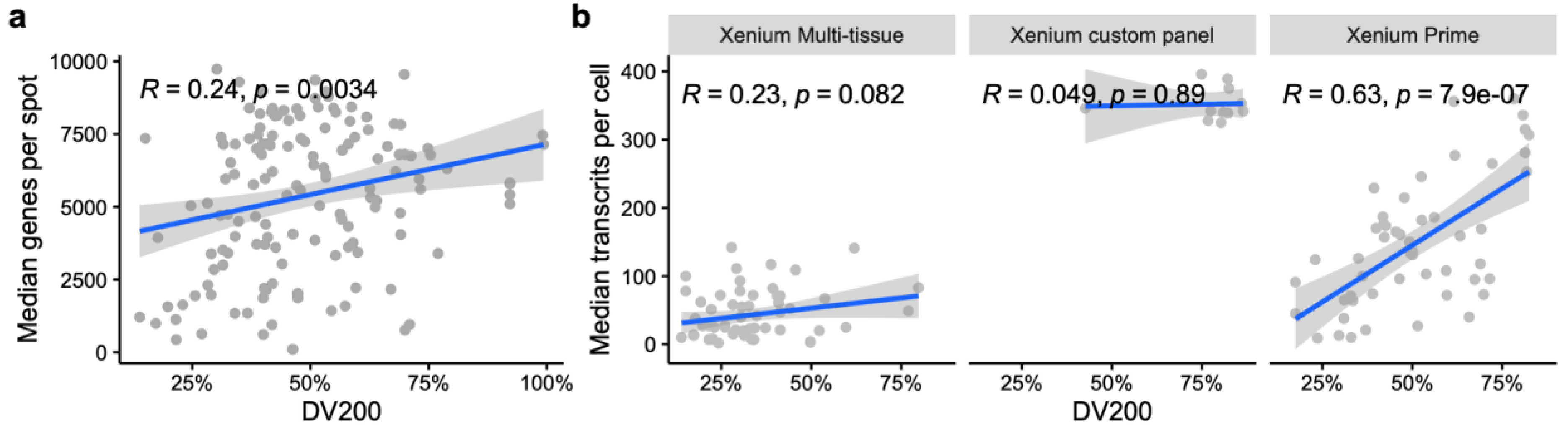
Figure 5. Selecting the right Xenium panel. a) Median-transcripts per cell (y-axis) obtained in two bladder cancer samples analyzed with the Xenium multi-tissue (gray) and Xenium Prime (orange) panels. b) Ratio between the median transcripts per cell obtained in a Xenium experiment and the gene panel size (y-axis) depending on the type of Xenium panel (x-axis). c) Correlation in the number of median transcripts per cell between technical replicates using the Xenium multi-tissue panel.

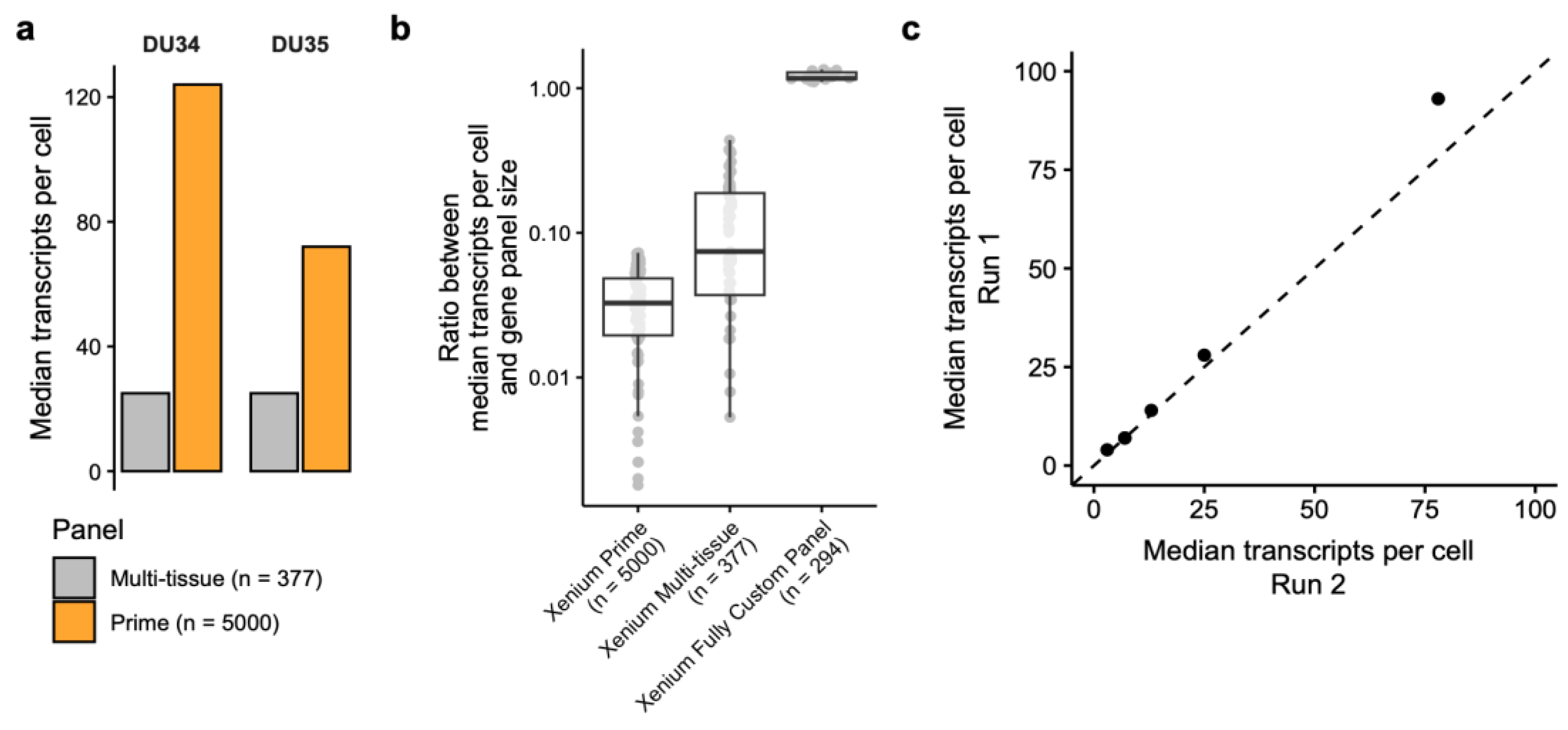
Figure 6. Sequencing saturation of Visium libraries. a) Distribution of the mean reads under tissue per spot for our collection of Visium cancer samples (n = 137). The vertical black dashed line shows the recommended minimum number of reads per spot by 10x (n = 25.000). b) Relationship between the mean reads per spot (x-axis) and the median genes per spot (y-axis). There is no correlation between both variables. c) Relationship between sequencing saturation (y-axis) and the number of reads per spot (x-axis), depending on the DV200 of the FFPE block. The vertical dashed line shows the minimum recommended sequencing depth by 10x (n = 25.000 reads per spot), and the horizontal dashed line the 70% saturation level. The red rectangles are areas with samples that have not been sequenced enough. Based on this, we recommend a sequencing of >100.000 reads per spot for Visium libraries from samples with DV200 above 30%.

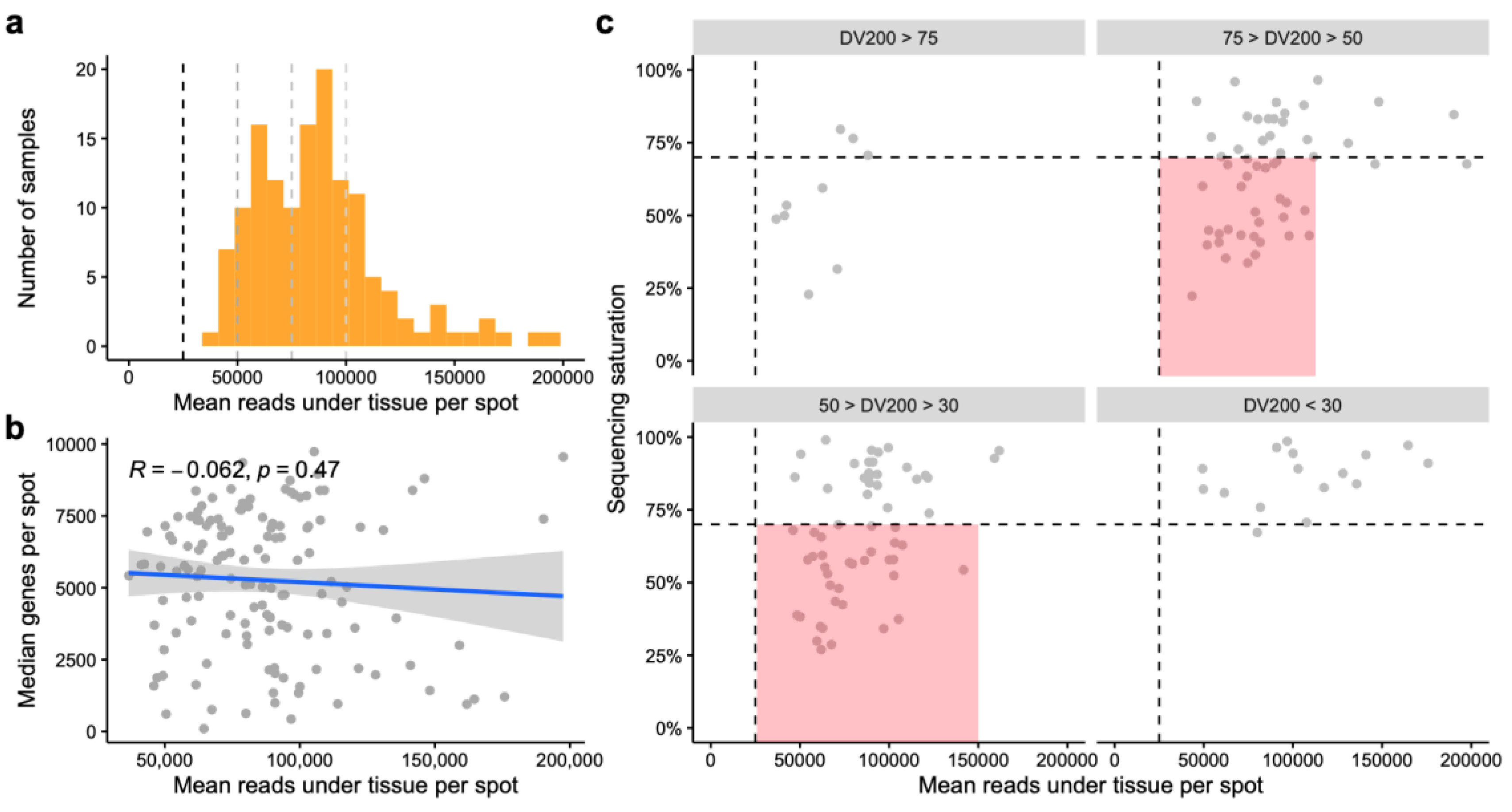
Table 1. Overview of current spatial transcriptomics platforms.

Platform (Type)	Resolution & Panel Type	Sample Types	RNA Quality	Best Use Cases
Visium (FF, sequencing)	~55 µm; Whole transcriptome	Human, mouse, all species (polyA+)	RIN ≥ 7 (≥ 4 w/ CytAssist)	Broad discovery in fresh tissue
Visium FFPE (sequencing)	~55 µm; Whole transcriptome	Human, mouse FFPE	DV200 ≥ 50% (≥ 30% w/ CytAssist)	Archived samples; full profiling
Visium HD (sequencing)	~2 µm; Whole transcriptome	Human, mouse FFPE or OCT	RIN ≥ 4; DV200 ≥ 30%	High-res + whole transcriptome
Xenium (imaging)	Subcellular; Targeted (up to 5000 genes; customizable)	Human, mouse FFPE or fresh-frozen; non-model (custom)	DV200 ≥ 10%	Cell typing; high-res profiling; cross-species (custom panels)
CosMx (imaging)	Subcellular; Targeted (up to 6000 genes)	Human, mouse FFPE or fresh-frozen	DV200 ≥ 10%	Multiplexed profiling; spatial cell state mapping
MERFISH / seqFISH (imaging)	Subcellular; Highly multiplexed (customizable)	Fresh-frozen; FFPE (with optimization)	Protocol-dependent	Deep profiling in microscopy-capable labs
Stereo-seq (sequencing)	500 nm; Whole transcriptome (species-specific probes)	Human, mouse, non-model (custom probes)	RIN ≥ 7 recommended	Nanoscale mapping; large area profiling
Non-model species	Varies by platform & probe design	Visium (polyA+), Xenium, Stereo-seq	Variable	Cross-species studies (requires custom panels or transcriptomes)

Disclaimer/Publisher’s Note: The statements, opinions and data contained in all publications are solely those of the individual author(s) and contributor(s) and not of MDPI and/or the editor(s). MDPI and/or the editor(s) disclaim responsibility for any injury to people or property resulting from any ideas, methods, instructions or products referred to in the content.

© 2025 by the authors. Licensee MDPI, Basel, Switzerland. This article is an open access article distributed under the terms and conditions of the Creative Commons Attribution (CC BY) license (http://creativecommons.org/licenses/by/4.0/).

Copyright: This open access article is published under a Creative Commons CC BY 4.0 license, which permit the free download, distribution, and reuse, provided that the author and preprint are cited in any reuse.