Submitted:
19 May 2025
Posted:
19 May 2025
You are already at the latest version
Abstract
Predicting basketball game outcomes is complex as every game is influenced by many factors including individual players’ performance and health conditions, team dynamics, team strategies, and game conditions. This study aimed to develop a machine-learning approach using game logs, player statistics, and historical data from the 2023–24 and 2024–25 NBA seasons. It incorporated game conditions and momentum indicators and optimized an XGBoost model using team-based train-test-validation, feature selection, and hyperparameter tuning. Key predictors included win streaks, home-court advantage, shooting efficiency, and player trades. SHAP values were used to interpret feature importance. The results suggest momentum, player performance, and rest days significantly influence game outcomes.
Keywords:
National Basketball Association (NBA)
; Sports Analytics
; Game Outcome Prediction
; Player Performance
; Game Conditions
; Machine Learning
; Feature Selection
; XGBoost
; Classification
; Hyperparameter Optimization
; SHAP
; Explainable AI
; Win Streaks
; Home-Court Advantage
; Rest Days
; Player Trades
; Accuracy
; F1 Score
; ROC-AUC
1. Introduction
The National Basketball Association (NBA) is one of the largest sports organizations in the world. Across the season, the data related to players, games, and teams are rapidly updated. However, due to the inherent nature of team sports, the game results depend on the various factors. This study leveraged machine learning techniques to identify the key factors that influence game outcomes. Specifically, the study investigated which game conditions and player metrics are the key factors that contribute to the predictions. The input data were game logs and individual player performance from the 2024-25 season as of 01/05/2025, overall player performance during the 2023-24 season, and player metadata, including height and years in the league. The variables included win streaks, home-court advantage, shooting percentages, and historical performance were used as model inputs to build a comprehensive model that not only identified key predictors of game results but also provided detailed explanations of the predictions.
The XGBoost model was optimized through team-based train-test-validation split, five different random seeds, feature selection, and hyperparameter tuning. SHAP values were used to explain the contribution of each feature to the predictions and provide insights into interactions between factors. Through these techniques, the study explored how recent momentum, rest periods, and trade history contributed to the likelihood of winning a game. This approach provided a general framework that teams could implement to optimize their game strategy. This study also addressed limitations related to team and game environments and the non-linear relationships inherent in NBA.
2. Literature Review
Recent studies have shown growing interest in predicting player and game performance across different sports fields using various data. [1] applied XGBoost and Random Forest techniques and evaluated Division-1 women’s basketball using player, team, and seasonal performance. In the study, [1] integrated players’ stress, sleep, recovery, and in-game statistics using wearable gear in the model to quantify and predict the performance in depth. [2] applied Deep Reinforcement Learning (DRL) and developed a metric that explains the probability of scoring the next goal based on each hockey game in National Hockey League (NHL). [3] explored different machine learning techniques and learned that a radial-basis function neural network model accurately predicted specific abilities of female handball players such as counter-movement jumps, sprints, and shuttle runs. [4] also used the European soccer leagues match data from 2015 to 2018 and explored machine learning approaches to predict which teams in European soccer leagues would perform better or worse than the previous season, predict the game performance, and predict the champion of the season.
NBA is one of the largest sports leagues in the world and recent studies also explored various machine learning approaches to understand the key factors to predict the injuries or game outcomes. [5] used machine learning techniques to understand the patterns of injuries, especially for lower body muscles such as hamstring, quadriceps, calf, and groin. In the study, the key factors causing these injuries were previous injuries, previous concussions, age, and game performance metrics such as free throw rate [5]. [5] mentioned that the model input did not consider the post-injury routine, team strategies for the continuous care, or clinical data.
- [6]
- built a XGBoost model to predict the NBA game results using the game data from 2021-2023 NBA seasons. The study used the SHAP values to explain the predictions and revealed that the key indicators were field goal percentage, defensive rebounds, and turnovers [6]. [6] recommended exploring different factors such as team tactics, player injuries, and game schedule in future studies.
- [7]
- built two-stage XGBoost models using the game data from the 2018-2019 season to predict the final scores of the games. The study found that the important features were related to the team’s average performance such as rebounds, field goal percentage, free throw percentage, and assists [7]. [7] mentioned that the model input was limited to only one season and recommended using stable feature selection techniques and incorporating features such as opponent information and game schedules.
- [8]
- built the Maximum Entropy model using the game statistics such as three-points or two-points field goal percentage, free throw percentage, and rebounds to predict the outcomes of playoff games. In the study, the mean of the game statistics was calculated for the most recent six games prior to the game that was being predicted [8]. [8] noted that the first game was excluded from prediction due to the absence of the prior data. [8] also mentioned that the model did not include information around relative strengths between the teams, injured players, and coaches’ directions.
Across the recent studies, the models were generally good at predicting the injuries and game results. Most of the studies focused on the player or the team performance during the game as models’ key predictors. The limitations discussed considering more features such as injured players, team strategies, game conditions. Also, the recent studies did not seem to focus on systematic or manual feature selection processes. most of the models were also limited in providing optimal predictors and less focused on the interpretability of the predictions. Thus, this study focused on minimizing the gap in the previous studies and including additional features including game conditions based on the preceding games, interpretability of the predictions, and actionable insights.
3. Method
3.1. Data Collection and Preprocessing
This study used NBA game log data from the 2024-25 season, collected as of January 5, 2024. Multiple datasets were collected though an API including game-level information, individual player performance metrics, player metadata, and seasonal statistics. The study focused on the current season data to make sure the study provides timely insights because NBA games are fast-changing and highly time-sensitive.
Data were collected from nba.stats.com using an API. The game information included the result of the game (win vs. lose), which was used as a response variable in this study. The player performance metrics were collected for each game and included field goal percentage, free throw percentage, rebound, assist, steal, block, turnovers, and personal fouls. Initial correlation analysis was conducted to manually remove the highly correlated variables. This manual feature selection helped improve the model interpretability. For example, the total points and total minutes a player played during a game
were excluded. This is because key players typically play longer and score higher than bench players, which also reflects on other metrics like total points, field goal percentage, and free throw percentage. The player metadata included players’ heights and years in the league. Weights were excluded because they were highly correlated with height. Seasonal player data had two parts, including the previous season and the current season. The data from the previous season included the overall percentage of field goals, the percentage of free throws, rebound, assist, steal, block, turnovers, personal fouls, and if the player was traded in the previous season. The current season data included player’s age, player’s team, and if the player was traded in the current season.
Pre-processing included handling missing data, removing outliers, and encoding categorical features to reduce the noise in the data. Missing values for previous season stats including steals (STL_LAST_SEASON) and turnovers (TOV_LAST_SEASON) were set to 0. This could be related to new players or injured players who did not play in the previous season. This process helped avoid errors in the model training process. Whether or not the player was traded last season (TRADED_LAST_SEASON) was also set to 0 when the player was not traded in the previous season. The total minute each player played each game was calculated. The original variable included minutes and seconds, for example, 35:14. Thus, the original variable was converted to the seconds and converted to the total minutes by dividing by 60. Players who played less than 1 minute in a game
were excluded because the player scores were unlikely to be relevant to the overall game performance. Categorical variables such as team names, game identifiers, and player identifiers were encoded to be used in the machine learning models.
Feature engineering was conducted through creating new features, including height in inches, overtime indicator, rest days, home game indicator, and preceding game win streak, to provide additional context to the model and improve the predictive power. Appendix A shows the variables used in the final model. The correlation analysis was conducted to see the relationships between final variables before the model building stage.
The traded indicators for 2024-25 and 2023-24 seasons were created to see if a player was traded. This was expected to show the trade impact on the team in the model. The career stats were pulled for each player. Players with the team name ’TOT’ (Total) indicated as the players had been traded mid-season by showing total stats across the two teams (previous team and traded team).
The heights were recorded as feet and inches. Thus, the variable was converted to inches to be used in the machine learning models.
The overtime indicator was to understand if an overtime game makes outcomes harder to predict due to the narrow scoring margins. Any game time with more than 240 minutes (minutes per player on the court) in the data was encoded as 1. 240 minutes represents minutes per player on the court.
There are 5 players on the court per team and 12-minutes quarters.
The rest days counter was used to understand the level of team’s fatigue. It was less precise compared to the wearable data. However, it was the best available estimate of fatigue level assuming all other factors including training routines are the same. First, the game log was sorted by game date for each team. Then, the difference between consecutive games was evaluated. The first game for each team did not have the preceding game to compare. Thus, rest days for these games were set to 0.
The home game indicator was created to see if teams are more familiar with their home stadium and how this would impact the game results. In the game-related data, the game match variable showed if the game was a home game (NYK vs. BOS) or away game (NYC @ BOS, which means New York team at Boston’s stadium). Thus, if the variable included ’vs.’ the game was encoded as a home game (1), otherwise as an away game (0).
The preceding game win streak was to understand if the consistent recent wins would impact the current game outcome. First, the data were sorted by team identifier and the game date to get the chronological order. For each team, a counter was generated to track the consecutive wins. If the current game result was ’W’ then the counter added 1 and if the current game result was ’L’ then the counter was reset to 0. This variable was appended as a new column for each team and the game. For the previous game win streak, the variable for the current game was shifted down by one game for each team. The first games of the season were set to 0 because these games did not have any previous game results.
The game identifier and player identifier were encoded as the model inputs to make sure each record represented a player and a game, which helped prevent data leakage. This helped the model link the player performance, game condition, and results during the training process. In the testing and validation, the model would see similar patterns in previously unseen players and games.
The data were split into training, validation, and test for the final model. The training set included all the teams except Boston Celtics and New York Knicks, the validation set included only Boston Celtics player and game data, and the test set included New York team player and game data. The split was to evaluate the model’s ability to generalize across different teams. As a result, the proportion for training, test, and validation datasets were was 93%, 3%, and 3% respectively.
The team names were excluded from the model inputs because the model tended to prioritize the higher-performing teams such as Cleveland Cavaliers and Oklahoma City Thunder. Thus, the model was overfitting towards to the performance patterns of these teams using the training set and made it less generalizable when testing and validating on the new sets of data. This also helped the model become less dependent on the team strategies, which was difficult to measure with the current data inputs. Thus, the model was set up to learn the general patterns from the overall player statistics and games-related data without team indicators and predict the game outcomes for specific teams.
3.2. Model Selection and Training
The models were built with XGBoost Classifier and optimized to predict the game outcomes. The final model used only the XGBoost model due to the time limitation. Future suggestions included considering different models to compare and improve model performance. Initially, the base model
without optimization was constructed to compare the performance with the optimized model. Then, another model with five random seeds and hyperparameter tuning process, but without systematic feature selection and train-test-validation split strategy. The train-test-validation split was not based on teams but rather on overall player and game data. Lastly, the final model with five random seeds, hyperparameter tuning, systematic feature selection, and a team-based train-test-validation split outperformed the rest of the models.
Five random seeds were generated with a reproducible process. The word "NBA" was converted into a unique large number using the MD5 hashing algorithm provided by the hashlib package. This large number can be linked back to the original input string ’NBA’. The large number was then used to feed the random number generator using the random package. Because this large number was unique, the generated random numbers were reproducible as long as the first input string was the same. Then, ten random numbers were generated within the range of 0 to 2,147,483,647. The first five random numbers were 1578879816, 1978497697, 1190903919, 1878057853, and 1288653849, and were used as seeds for 5 different runs.
The Optuna package was used to automate feature selection and hyperparameter optimization [9]. In this study, an Optuna study object ran 20 trials to search for the best combination of hyperparameters and features. The study was run with five different random seeds to improve the stability of the model predictions. Within Optuna study object, the process involved four steps including feature selection, initial model training on selected features, hyperparameter optimization, and final model testing.
Various ranges of hyperparameters were considered including the number of parallel trees, maximum tree depth, learning rate, subsample, features sampled for each tree, minimum child weight, gamma, alpha, and lambda [10]. The optimal number of trees was explored in a range from 50 to 500. Less than 50 trees would introduce high bias and more than 500 trees would introduce overfitting [10]. [11] compared the XGBoost model performance across 24 different datasets and the models that produced the highest prediction accuracy were observed when the models used a number of trees in the range of 50 to 500.
The optimal depth for individual trees was explored in a range from 3 to 100 to balance the model complexity. Low tree depth would introduce high bias and high tree depth would introduce overfitting [10]. The optimal learning rate was explored in a range from 1 × 10⁻³ to 1 × 10⁻¹ to balance the learning speed, as the lower learning rate helps the model to learn stably but slowly and the higher learning rate helps the model to learn faster but less stably [10]. The optimal subsample and feature sample for each tree were also explored with a range from 0.2 to 1.0. 0.2 means that the individual tree uses a randomly selected 20% of the training dataset or features, while 1.0 means that the individual tree uses the entire train dataset or features to grow the tree [10]. Using a portion of the train dataset or features would run the model faster but be prone to high bias and using the entire train dataset or features would be slower to run and prone to overfitting [10]. Minimum weight for child node was explored from a range from 1 to 10. The higher minimum weight makes it harder to further split the child node and leads to lower risk of overfitting, while the lower minimum weight makes it easier to further split the child node and leads to higher risk of overfitting [10]. Lastly, the optimal gamma, alpha, and lambda were explored with a range from 1 × 10⁻⁹ to 1.0. The higher value for these parameters represents more regularization [10]. Appendix A summarized final values for hyperparameters that Optuna determined across the five random seeds.
To select the most predictive and relevant features, the XGBoost model was trained with the best parameters selected through the Optuna study on the training dataset. Then, features were selected if their importance scores exceeded the average importance score of all the features. The maximum number of features was limited to 20 to improve model interpretability. The selected features were stored for later processes, including training, testing, and validating the model as well as stability analysis.
With the best-selected features, the Optuna study ran 20 trials again to find the best combination of hyperparameters. The parameters included learning rate, maximum depth, number of estimators, subsample ratio, column sampling per tree, minimum child weight, and regularization factors included gamma, alpha, and lambda. The scale_pos_weight parameter was set as 0.7 to maximize the F1 negative score. The goal of the optimization was to maximize the F1 negative score to balance positive and negative predictions.
In the final model training process, the train and validation sets were merged and filtered to keep only the best-selected features. The final XGBoost model was trained using the best hyperparameters from the Optuna study. Then, the final model was evaluated on the test set that the model had never seen.
3.3. Model Evaluation and Validation
The model performance metrics were generated, including Accuracy, F1 Score, Sensitivity, Specificity, ROC-AUC, and a confusion matrix. The accuracy explains the percentage of correctly predicted outcomes. F1 positive score evaluates how well it predicts the positive classes using precision and recall, while the F1 negative score evaluates performance for negative classes. Specificity explains the ability to correctly identify negative classes, while sensitivity explains the ability to correctly identify positive cases. ROC-AUC measures the ability to distinguish between classes. Additionally, the confusion matrix was constructed to assess model performance.
These metrics were evaluated for each of the five model runs using different random seeds. The mean, median, and variance of these metrics were then calculated across the five runs to evaluate overall model performance. Compared to the base model, the optimized XGBoost model showed significant improvements in F1 negative score.
3.4. Feature Importance and Interpretation
Stability analysis was conducted to see how often each feature was selected across five different seeds. The features selected in the most trials were considered stable and important features.
SHAP (Shapley Additive Explanations) values were evaluated, including the feature importances and the individual SHAP values across the 5 models. The SHAP summary plots showed the distribution of SHAP values across all the observations in order of feature importance. It is important to note that the summary plots only show the influence of each factor on the predictions. The SHAP interaction plots showed the impact of a feature on the prediction and the possible interactions with another feature in color. It is also important to note that these interactions are only between two features and other factors could be influencing the outcome. The SHAP force plots provided a detailed example of how a player’s performance and game conditions influenced the game results.
4. Results
4.1. Data Exploration
The final dataset included 9,547 combinations of player and game statistics. Across the 9,547 rows, 4,801 (50%) were wins. The data included 517 games and 445 players across 30 teams. 326 (3%) of them were related to games played by the Boston Celtics team and were used as a test dataset. 341 (3%) of them were related to games played by the New York Knicks team and were used as a validation dataset. The rest of the records about 8,880 (93%) were used as the training dataset. Only 25 games out of 517 games (5%) went to overtime.
The trade information was included across 2024-25 and 2023-24 seasons. Figure 1 summarized the distribution of the variables. There were more players traded in the 2023-24 season about 8% because the data included the whole season trade information, while the trade information for the 2024-25 season was only as of January 5th, 2025, which was one month before the trade deadline of February 5th, 2025. NBA teams usually make more trades close to the trade deadline. Thus, only earlier trade information for the 2024-25 season was included in the data.
The players’ heights showed the physical characteristics of the players in the data. Figure 2 showed that the distribution was normally distributed with a mean of 79 inches (6 feet 5 inches) and a median of 78 inches (6 feet 5 inches). As mentioned earlier, the heights were converted into inches to be used as a machine learning model input.
Figure 3 summarized the distribution of other variables that were feature-engineered. Figure 3a showed the distribution of the teams’ rest days before each game in the 2024-25 season. Most of the time (56%) teams had a 2-day rest days period, which could be intentional by the NBA organization for the teams to rest. However, 20% of the time teams had back-to-back games or had only one day of rest, which seemed to be less ideal for the players especially given that each game is intense.
Figure 3b showed the distribution of the win streaks that a team had before each game. Half of the time (52%) a team had a 0-game win streak, which indicated that each game has a loser team and a winner team, otherwise the game continues with the overtime policy. It was very rare that teams had more than 9 preceding-game win streak. The right tail showed Cleveland Cavaliers, who won 15 times in a row by November 17th, 2024, and Oklahoma City Thunder team, who won 14 times in a row by January 5th, 2025.
Figure 4 summarized the correlation between final variables. In general, overall performance metrics from the previous season were highly correlated with each other. For example, field goal percentage and free throw percentage were highly correlated because both metrics reflected shooting skills. Additionally, the performance was aggregated over the previous season and reduced the noise across multiple games. Thus, the stats from the last season were more highly correlated than the stats from the current season because these reflected the players’ performance for each game, which included noise such as bad performance days or injured days. Performance between current and last season was also positively correlated, which showed the consistency in performance across the seasons. Years in the league and the player age showed a positive relationship because older players tend to have more years in the league. Assist showed an inverse relationship with height. This could be because shorter players tend to initiate the offense and pass to the taller players who are usually near the basket. The target variable ’W’ did not have a clear correlation with the final variables. It is important to note that this correlation analysis was for data exploration purposes. Thus, this study employed machine learning models with systematic feature selection and SHAP values to understand the predictions.
4.2. Model Performance
Initially, the base model without any feature selection and hyperparameter tuning processes was constructed. Table 1 summarized the performance of the base model using accuracy, F1 positive and negative scores, specificity, sensitivity, and ROC AUC. The base model performed worse when predicting losses with an F1 negative score of 66%. Table 2 summarized the stacked confusion matrix across the validation and test sets and showed that the base model correctly identified 439 negatives out of 521 (84%) and 107 positives out of 146 (73%). Thus, the later models were optimized to maximize the F1 negative score to improve the model’s ability to balance the predictions and provide a more generalizable recommendation for game and player strategy.
Then, another model was explored using five random seeds and a hyperparameter tuning approach. However, this model was randomly split 20/80, instead of team-based train-test-validation split, and did not consider systematic feature selection. Table 3 summarized the performance across the five seeds. The overall accuracy was 64% and the F1 negative score was 63%. Table 4 showed similar counts of false negatives and false positives. Not having the team-based train-test-validation split and feature selection significantly reduced the model performance. The random splitting approach may have caused data leakage because both training and test set might have been from the same team. Additionally, the model could have employed irrelevant features due to the lack of a feature selection process. Thus, these findings recommended using the team-based data split to prevent the data leakage and a systematic feature selection process to reduce noise. As a result, the Boston Celtics and New York Knicks were selected as the held-out teams for the test and validation sets.
Based on the findings from the initial models, the final model was optimized through feature selection and a hyperparameter tuning process, with a team-based train-test-validation split. Table 5 summarized the model performance across five randomly selected seeds. Overall, the mean accuracy (87%) and F1 negative score (83%) showed significant improvement compared to the initial models.
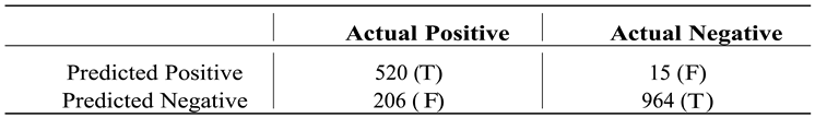
Table 6 summarized the stacked confusion matrix across five randomly selected seeds. The confusion matrix showed that the models correctly identified negative cases about 964 times out of 979 (98%) with fewer false positives. However, the model was incorrectly identified positive cases about 520 times out of 726 (72%) and more false negatives.
Figure 5 summarized how many times these features were selected during the feature selection process across five different seeds. Seventeen features were selected 100% of the time, while block (BLK) and field goal percentage (FT_PCT) were selected 80% of the time (4 out of the 5 runs). This emphasized the high stability in the importance of these features across five different runs.
4.3. Model Interpretation
Figure 6 summarized the SHAP values for each data point and their impact on the model’s outcome ranked by feature importance. The most important features for predicting game outcomes were the win streak prior to the game, home-court advantage, field goal percentage, and the previous season’s steals, field goal percentage, and free throw percentage. Other features had relatively smaller impacts and none of the individual player and game indicators were considered important. Among the variables, the win streak leading into the game was the most influential factor.
A longer win streak entering the current game was strongly associated with a higher predicted win probability. This suggested that teams with recent winning momentum and established success contribute significantly to their chances of winning.
Home-court advantage also had a substantial impact and emphasized the importance of stadium familiarity and local fan support. Higher field goal percentages generally led to a higher predicted win probability, but even moderate percentages could sometimes have a positive effect. The moderate percentage may reflect the non-linear nature of player performance where bench players stepped up while key players were underperforming or dealing with injuries.
Metrics from the previous season, such as steals, field goal percentage, and free throw percentage, also played a significant role. Strong steal and field goal percentages from the previous season tended to contribute to a team’s success. This implied that established defensive and offensive skills carried over to the next season. The impact of free throw percentage was more nuanced. This could be because free throw percentage was more dependent on individual player performance and could be improved through dedicated practice.
The interaction plot showed potential relationships between features. Figure 7 showed that a longer win streak increased the likelihood of winning the game. Additionally, this effect was stronger with home games when the team started hitting 4-game win streak, while the effect was less effective at a three-game streak. This implied that when a team had enough momentum, being at home court could significantly increase the likelihood of winning the game, which further emphasized synergistic effect between winning-streak momentum and home-court advantage.
Figure 8 showed the interaction between overtime games and the preceding game’s win streak. The distribution of overtime games was relatively sparse due to the low sample size. Additionally, no clear relationship was observed between overtime games and win streaks. However, when the game ended without overtime, a clear positive correlation was identified where the longer win streaks, at least a 4-game streak, were associated with a higher likelihood of winning the game, which aligned with Figure 7. This also emphasized how difficult game results were to predict during overtime games.
Figure 9 showed a clear negative relationship between whether a player was traded last season and the game outcome. This implied that the players would need time to adjust to a new team environment and find the best-fit role in the new team. This could be a selection bias as teams often trade players who are underperforming or not fitting the team’s needs. Thus, more support and integration strategies would be needed for newly traded players to increase the probability to improve win probability.
As shown in Figure 10a, home games were highly associated with winning, and teams with two days of rest also showed a higher likelihood of success. This combination of a 2-day rest period and a home game appeared to be beneficial because players could avoid the fatigue and disruption caused by travel and they could follow a consistent routine while they were staying at home. While it might seem intuitive that longer rest periods would be ideal, this finding suggested that a balance between rest and maintaining competitive momentum was crucial. Specifically, as shown in Figure 10b, a 2-day rest period appeared to provide sufficient recovery time for players during the home game and more recovery time around 3 or 4 days while they were traveling seemed beneficial. This further emphasized the importance of balancing recovery time and maximizing home-court advantage.
Figure 11a showed the interaction between field goal percentage and turnovers in the previous season. There was a clear positive relationship between field goal percentage and its impact on the likelihood of winning. However, the interaction with turnovers from the last season was nuanced. Some players with a higher number of turnovers in the previous season tend to be those who had greater ball possession. Since teams typically trust their best players with the ball, it is reasonable to observe that some of the players with high turnovers in the last season had high a field goal percentage in this season. Thus, a higher turnover rate from the last season was more likely to contribute positively to a team’s success. This aligned with Figure 11 where there was a positive relationship between assists in the current season and turnovers in the last season and their impact on the likelihood of winning. The players with the higher turnovers in the previous season, who were most likely a key player with high field goal percentage and assists, seemed to have more experience with the ball and higher chance to assist and help the team win the game.
However, some players had lower field goal percentages and higher turnovers during the last season. This explained not all the key players in the previous season had a good field goal percentage this season. This suggested when looking for players who not only take possession but also have the potential to score efficiently, considering not only their turnover rate from the previous season, but also other factors such as field goal percentages or assists during the current season could be helpful.
Figure 12 and Figure 13 showed how player OG Anunoby on the New York Knicks influenced the game outcomes in their matches against the Indiana Pacers on October 25th, 2024 and November 10th, 2024. In both games, his strong performance from the previous season and his field goal percentage above 50% positioned him as a key player. These factors positively impacted the model prediction. However, the key difference between these games was home-court advantage. Playing at the home on October 25th, 2024 contributed to a win, while the away game on November 10th, 2024 against the same team contributed to a loss.
The most recent matchup that New York Knicks had in this data was with Chicago Bulls on
January 04, 2025. Figure 14 showed how player OG Anunoby influenced the game outcome in this match. The limited rest days without the home-court advantage and less winning momentum had negatively impacted the game results, while last season’s performance still seemed to be remained a helpful factor. If he were to have better game conditions with at least two days of rest and home-court advantage and positive winning momentum, his impact could have been more powerful to help his team win.
5. Conclusion
The overall model accuracy was 87% with a F1 positive score of 90% and a F1 negative score of 83%. However, the high false negatives (206) in the confusion matrix showed that the model overestimates winning cases. Feature selection was stable across the five different seeds.
The SHAP summary plot showed the most influential variables in predicting game outcomes, including win streak before the game, home game indicator, field goal percentage, and the last season’s statistics, such as steals, field goal percentage, free throw percentage.
SHAP interaction plots showed that longer win streaks increased the probability of winning, especially when playing at home. A team with a longer win streak and an overtime game also increased the probability of winning. Players who were traded in the last season showed a negative relationship with the game outcome. It is important to note that there could be a selection bias as those players are not the key players that form the strategy around. A 2-day rest period before a home game or A 3- or 4-day rest period before an away game was ideal to balance the recovery and momentum. The field goal percentages and assists increased the probability of winning. Some players had higher turnovers in the previous seasons had higher field goal percentages and assists, which suggested that they had higher ball possession in the previous season and they have been key players across the two seasons.
SHAP force plots showed how OG Anunoby’s performance and his game condition were influencing the game predictions. In each game, his strong performance from the previous season consistently positioned him as a key player to cntribute to a positive game outcome. However, the home-court advantage seemed to play a significant role across the different games.
6. Discussion
Predicting basketball game outcomes is challenging because basketball games involve various factors including players, team dynamics, coaches, referees, fans, trades, and external pressures. However, the model in this study mainly focused on the player performance and conditions and did not consider other factors that could also influence the game results. Additional data such as further historical data, coach formation, player fatigue levels or injury history, ball possessions, stadium conditions, opponent strength analysis, referee calls analysis, press conference sentiment for previous games, wearable data, and advanced offensive and defensive metrics could improve the model’s ability to build more precise strategies in addition to the game performance data used in this study.
The high specificity (98%) showed that the model performs well at identifying true losing cases, while the confusion metrics showed that the model is less effective when predicting positive cases with 82% overall sensitivity. This could be from less predictive features or the model’s optimization strategy, which prioritizes negative cases. Factors such as setting a parameter to adjust the balance between positive and negative classes as 0.7 (scale_pos_weight) and optimizing for negative class performance could have contributed to the imbalanced performance.
From the confusion matrix, high false negatives could be concerning because the model predicted that a team would lose when they actually win and this could lead to poor decisions by switching their effective strategies. However, this could also lead the team to discover innovative approaches and validate their strategies were effective. Whereas, having high false positives might cost the team more because often teams are overestimating and end up having unexpected outcomes during the important games, such as playoff matches. Thus, having a high number of false negatives might cost less, while having a well-balanced model would be a more robust approach in the future.
Future studies could focus on incorporating additional features, balancing the negatives and positives, and comparing options across different models to enhance model performance. It is important to note that integrating these SHAP values with additional causal tools would provide a more actionable recommendations for teams to develop their strategy. Using a controlled experiment or a causal inference technique would be helpful to understand the true impact of hypotheses that was suggested in this study and further provide actionable insights into winning strategies.
As a result, the model in this study provided a general understanding of the NBA basketball game outcome predictions around win streak and team motivation, rest day strategies depending on the home or away schedules, and influence of the last season’s data such as trade information and turnover statistics. Leveraging these insights, the future studies should incorporate more advanced techniques such as a controlled experiment and causal inference, more predictive features that could explain the complex dynamic of basketball games, and alternative models to provide more specific, actionable, and data-driven strategies for the teams.
Appendix A
The final variables included in the model were as follows (nba_glossary):
- Game ID – MIdentifier (0 or 1) for each game (i.e. GAME_ID_22400486 represents the game played on January 4th, 2025 with Atlanta Hawks and Los Angeles Lakers)
- Player ID – Identifier (0 or 1) for each player (i.e. PLAYER_ID_1629060 represents the player of LeBron James)
- Home – Identifier (0 or 1) for home game
- Overtime – Identifier (0 or 1) for over time game
- Rest Days – How many day(s) the team didn’t have a game prior to the current game date
- Previous Game Win Streak – How many game(s) the team consecutively won prior to the current game
- Field Goal Percentage – How many times the player made the goals compared to the goal attempted in the game (%). Last year overall performance is also available as an variable.
- Free Throw Percentage – How many times the player made the free throw goals compared to the free throw attempted in the game (%). Last year overall performance is also available as an variable.
- Rebound – How many times the player made the rebound for the game. Last year overall performance is also available as an variable.
- Assist – How many times the player made the assist for the game. Last year overall performance is also available as an variable.
- Steal – How many times the player made the steal for the game. Last year overall performance is also available as an variable.
- Turnover – How many times the player made the turnover for the game. Last year overall performance is also available as an variable.
- Personal Foul – How many times the player made the personal foul for the game. Last year overall performance is also available as an variable.
- Height – Player heights in inches
- Player Age – How long the player have been playing in the NBA league
- Traded this season – Indicator (0 or 1) for the player was traded in the season of 2024-25 before January 05, 2025
- Traded last season – Indicator (0 or 1) for the player was traded in the season of 2023-24

Table A1.
Optimal Hyperparameter Values Across Five Random Seeds.
| Seed | Parallel Trees | Max Depth |
Learning Rate |
Subsample | Feature Sample | |
| Seed 1 | 386 | 98 | 0.09 | 0.83 | 0.64 | |
| Seed 2 | 313 | 45 | 0.09 | 0.86 | 0.88 | |
| Seed 3 | 492 | 98 | 0.08 | 0.74 | 0.57 | |
| Seed 4 | 389 | 41 | 0.09 | 0.91 | 0.46 | |
| Seed 5 | 116 | 39 | 0.09 | 0.45 | 0.31 | |
| Seed | Min Child Weight | Gamma | Alpha | Lambda | ||
| Seed 1 | 6 | 6 × 10⁻⁷ | 7 × 10⁻⁶ | 0.003 | ||
| Seed 2 | 7 | 6 × 10⁻⁸ | 3 × 10⁻⁸ | 3 × 10⁻⁸ | ||
| Seed 3 | 8 | 3 × 10⁻⁵ | 0.003 | 0.002 | ||
| Seed 4 | 10 | 1 × 10⁻⁸ | 0.003 | 3 × 10⁻⁴ | ||
| Seed 5 | 8 | 1 × 10⁻⁸ | 0.001 | 0.060 | ||
References
- Taber, C.B.; Sharma, S.; Raval, M.S.; Senbel, S.; Keefe, A.; Shah, J.; Patterson, E.; Nolan, J.; Artan, N.S.; Kaya, T. A holistic approach to performance prediction in collegiate athletics: player, team, and conference perspectives. Scientific Reports 2024, 14. [Google Scholar] [CrossRef] [PubMed]
- Liu, G.; Schulte, O. Deep Reinforcement Learning in Ice Hockey for Context-Aware Player Evaluation. In Proceedings of the Proceedings of the 27th International Joint Conference on Artificial Intelligence (IJCAI), 2018, pp. [CrossRef]
- Oytun, M.; Tinazci, C.; Acikada, C.; Yavuz, H.U.; Sekeroglu, B. Performance Prediction and Evaluation in Female Handball Players Using Machine Learning Models. IEEE Access 2020, 8, 116321–116335. [Google Scholar] [CrossRef]
- Pantzalis, V.C.; Tjortjis, C. Sports Analytics for Football League Table and Player Performance Prediction 2020. pp. 1–8. [CrossRef]
- Lu, Y.; Patel, B.H.; Camp, C.L.; Forlenza, E.M.; Forsythe, B.; Lavoie-Gagne, O.Z.; Reinholz, A.K.; Pareek, A. Machine Learning for Predicting Lower Extremity Muscle Strain in National Basketball Association Athletes. Orthopaedic Journal of Sports Medicine 2022, 10, 232596712211117. [Google Scholar] [CrossRef] [PubMed]
- Ouyang, Y.; Li, X.; Zhou, W.; Hong, W.; Zheng, W.; Qi, F.; Peng, L. Integration of machine learning XGBoost and SHAP models for NBA game outcome prediction and quantitative analysis methodology. PLOS ONE 2024, 19, e0307478. [Google Scholar] [CrossRef] [PubMed]
- Chen, W.J.; Jhou, M.J.; Lee, T.S.; Lu, C.J. Hybrid Basketball Game Outcome Prediction Model by Integrating Data Mining Methods for the National Basketball Association. Entropy 2021, 23, 477. [Google Scholar] [CrossRef] [PubMed]
- Cheng, G.; Zhang, Z.; Kyebambe, M.N.; Kimbugwe, N. Predicting the Outcome of NBA Playoffs Based on the Maximum Entropy Principle. Entropy 2016, 18, 450. [Google Scholar] [CrossRef]
- Akiba, T.; Sano, S.; Yanase, T.; Ohta, T.; Koyama, M. Optuna: A Next-generation Hyperparameter Optimization Framework. In Proceedings of the Proceedings of the 25th ACM SIGKDD International Conference on Knowledge Discovery and Data Mining; 2019. [Google Scholar]
- Chen, T.; Guestrin, C. XGBoost parameter tuning documentation, 2020. Version 3.0.0.
- Wang, H.; Wu, Z.; Wang, X.; Bian, L.; Jin, H. HardGBM: A Framework for Accurate and Hardware-Efficient Gradient Boosting Machines. IEEE Transactions on Computer-Aided Design of Integrated Circuits and Systems 2023, 42, 2122–2135. [Google Scholar] [CrossRef]
Figure 1.
Distribution of Traded Players Across Two recent Seasons.
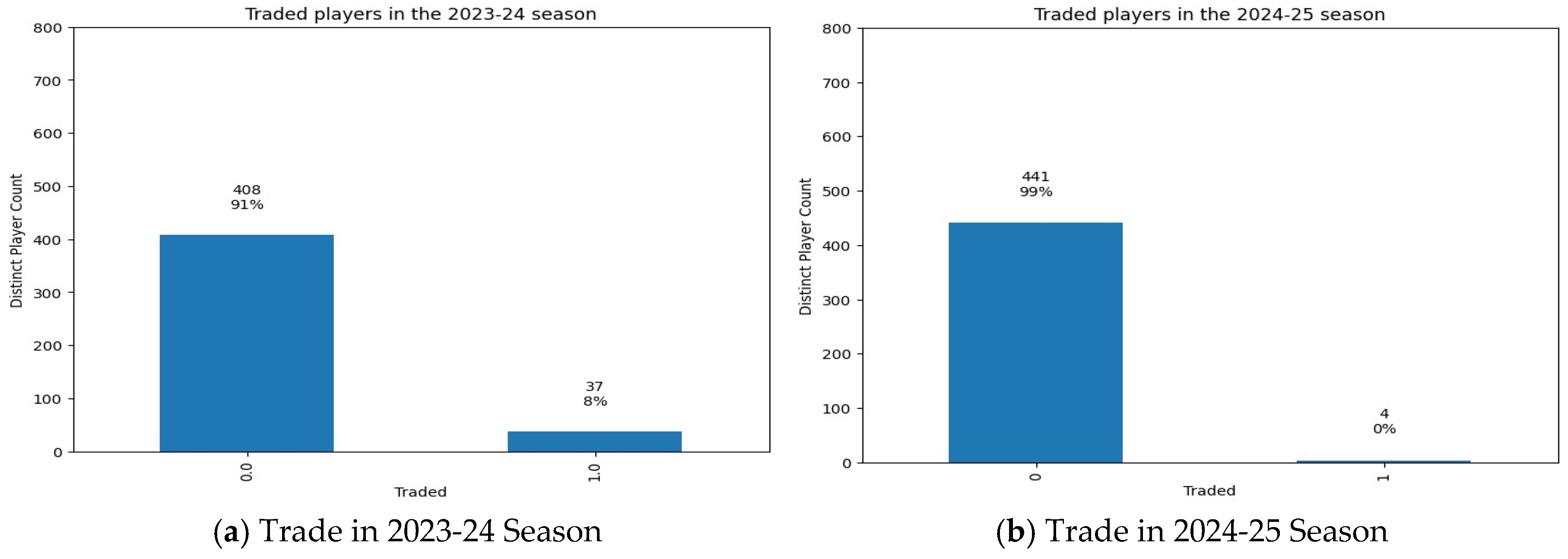
Figure 2.
Distribution of Players’ Heights in Inches.
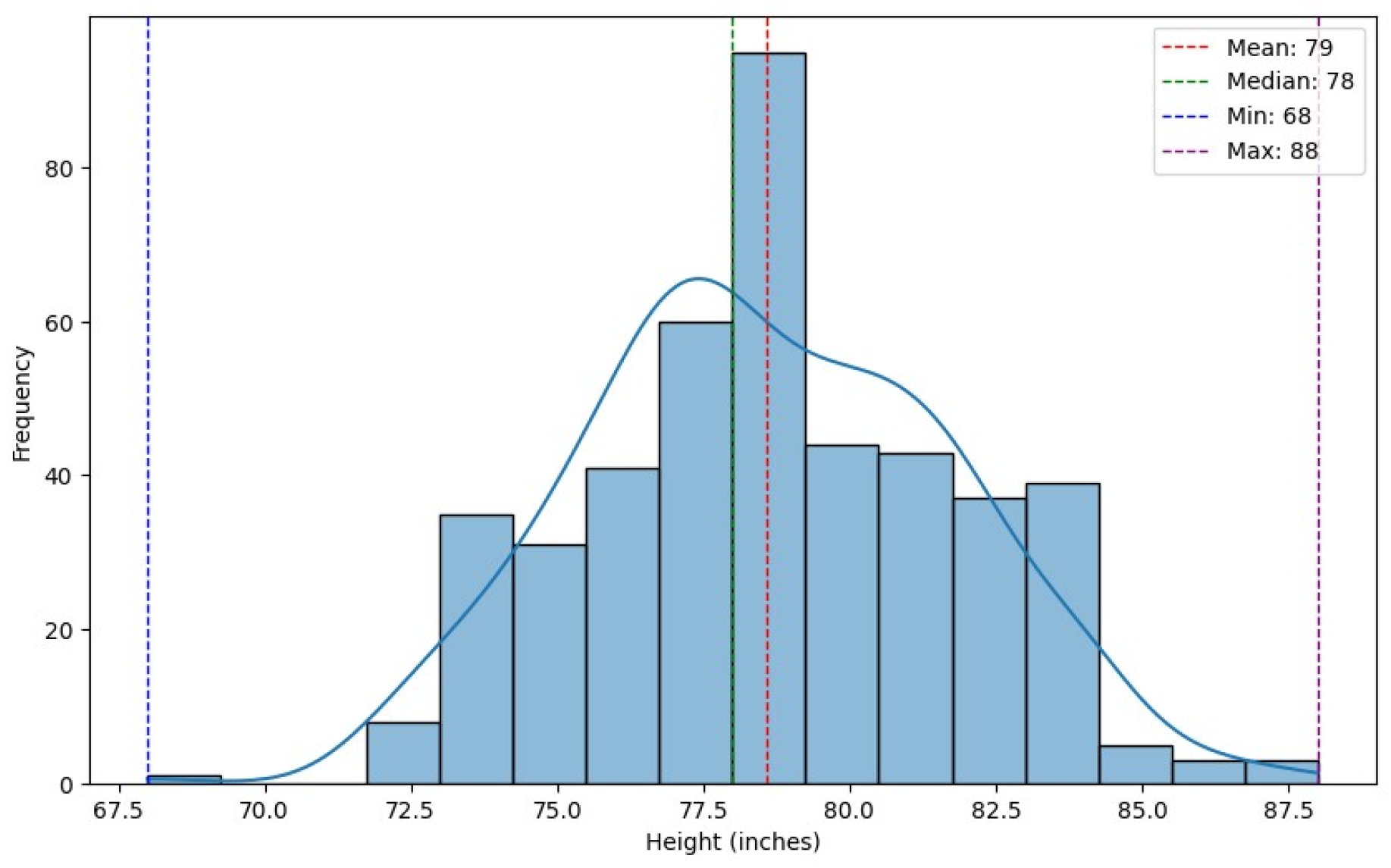
Figure 3.
Distribution of Other Variables.
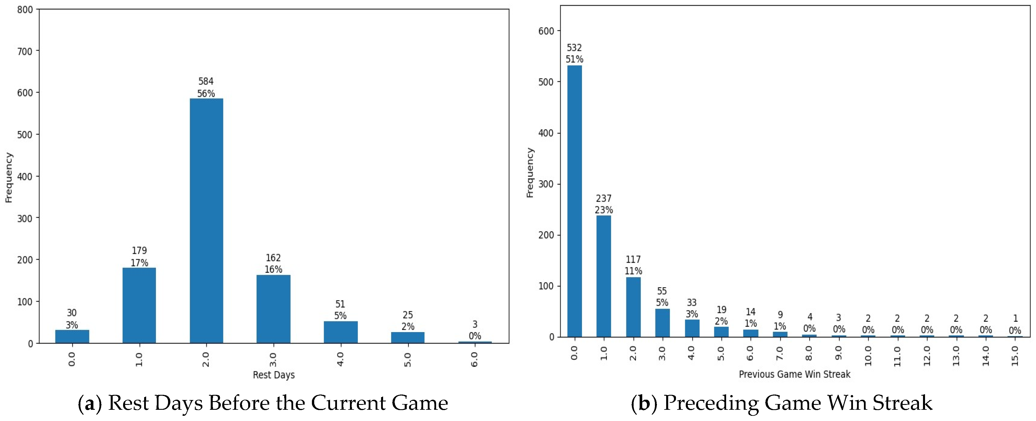
Figure 4.
Correlation Matrix across Final Variables.
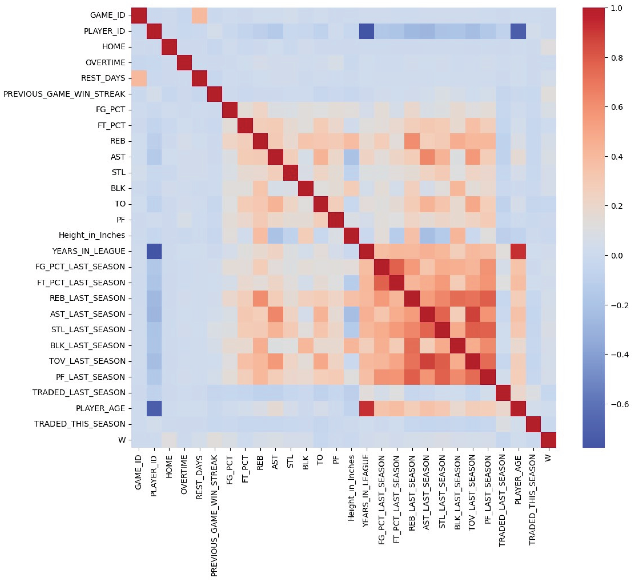
Figure 5.
Feature Selection Frequency Across Five Seeds.
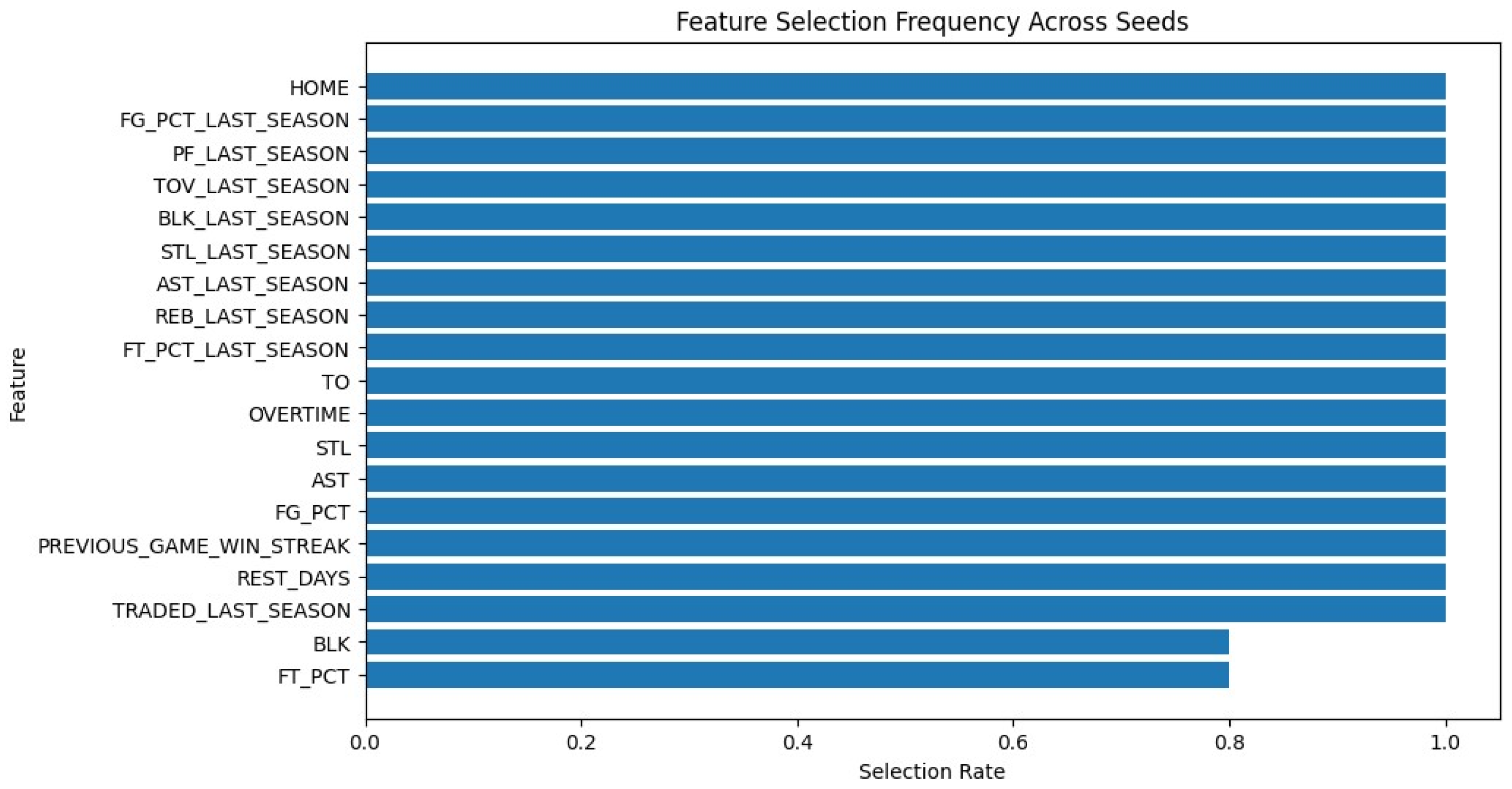
Figure 6.
SHAP Summary Plot.
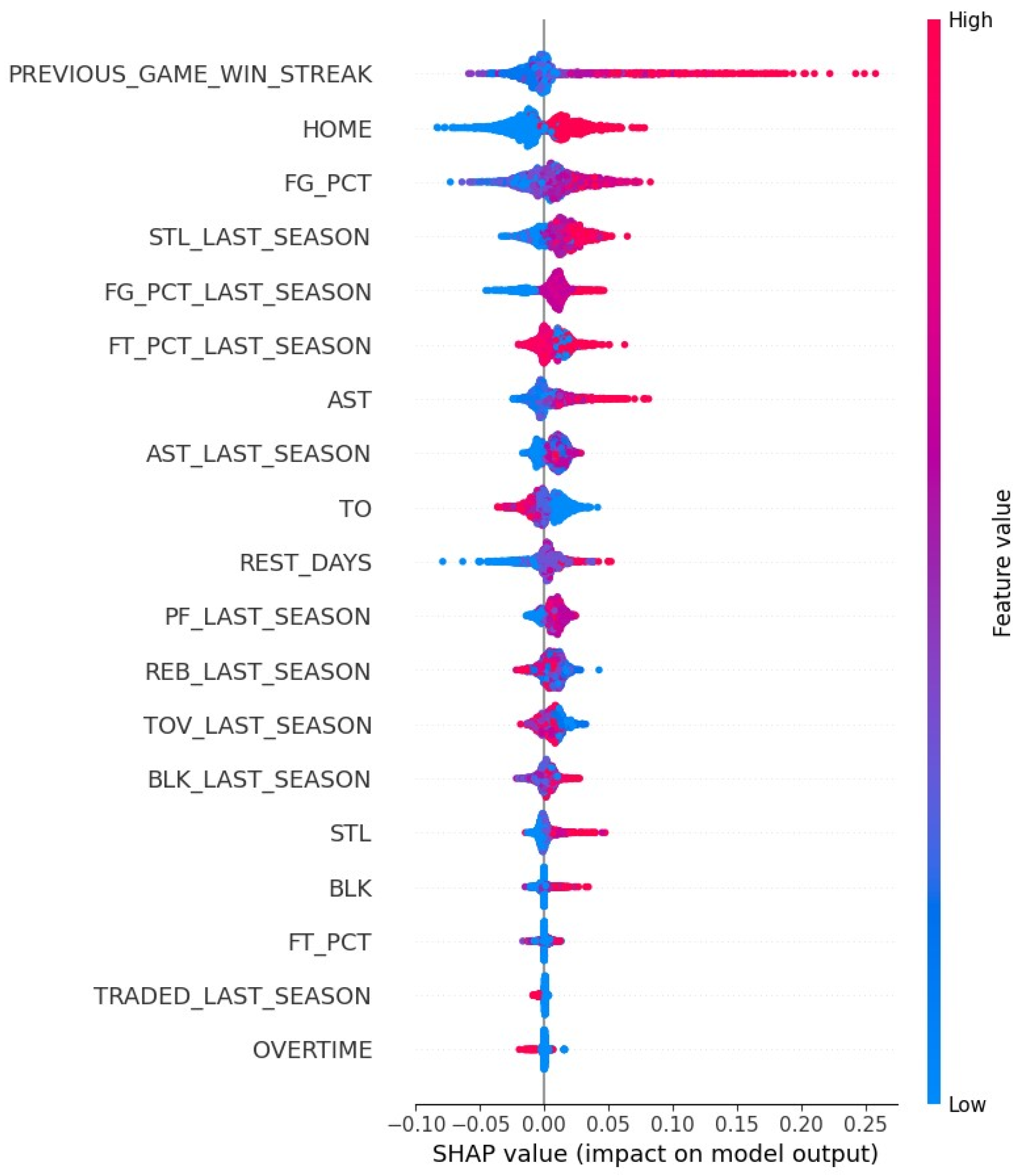
Figure 7.
SHAP Interaction Plot - Previous Game Win Streak.
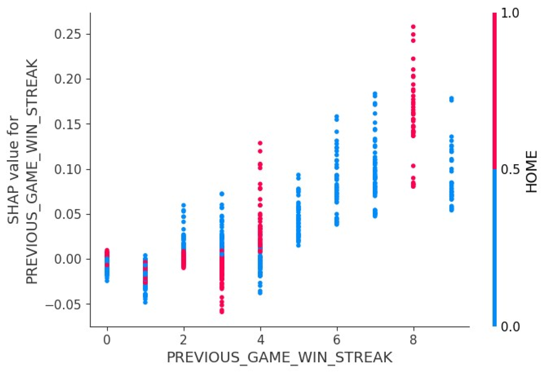
Figure 8.
SHAP Interaction Plot - Overtime.
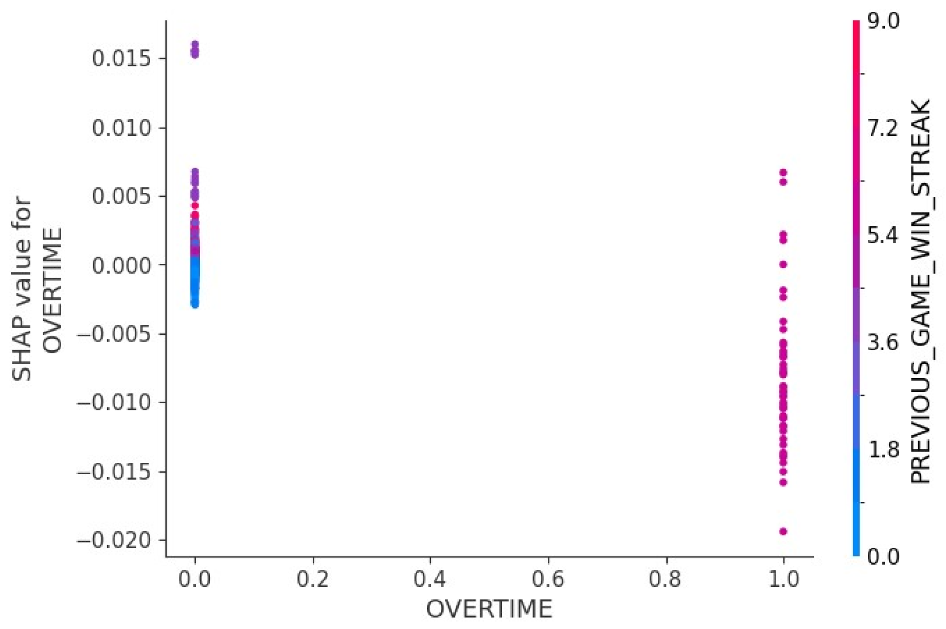
Figure 9.
SHAP Interaction Plot - Traded in the Last Season.
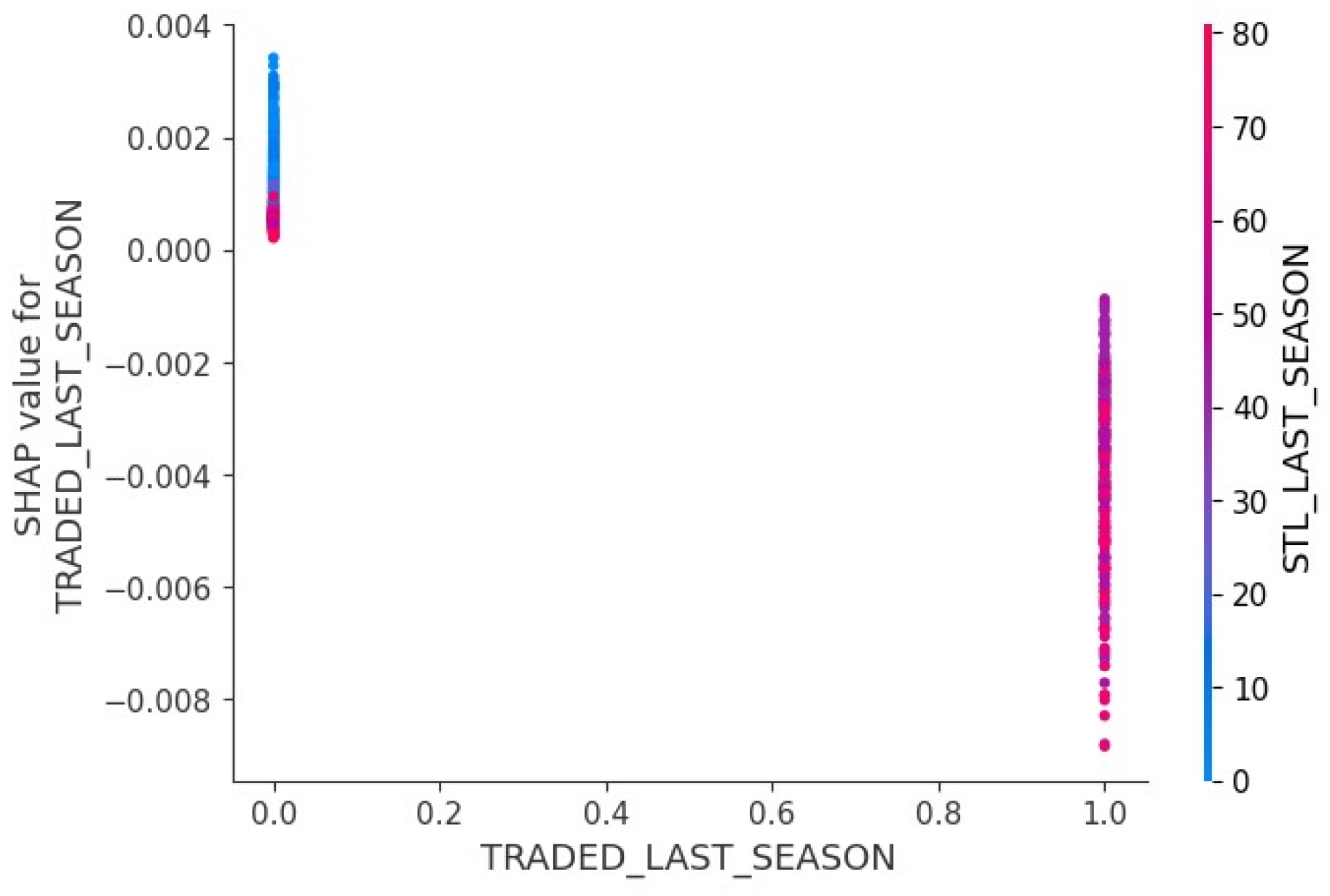
Figure 10.
SHAP Interaction Plot.
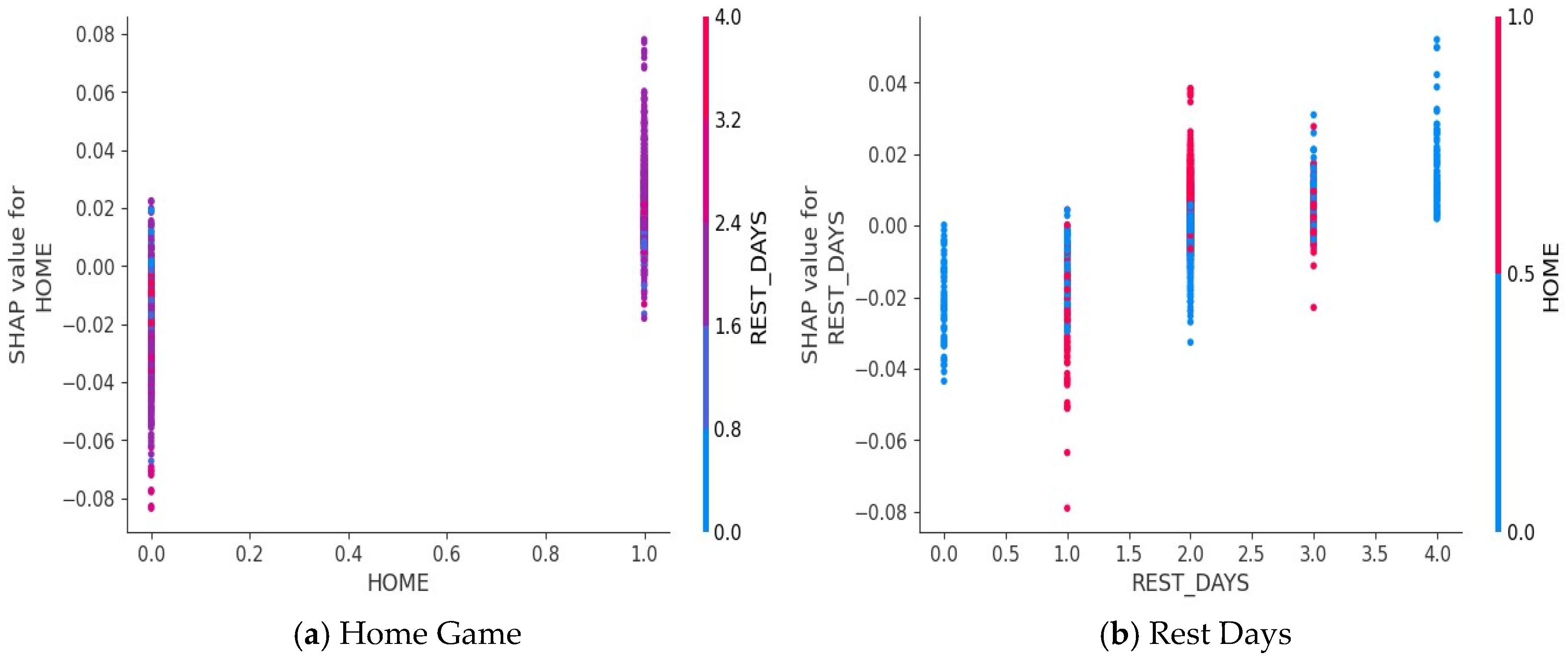
Figure 11.
SHAP Interaction Plot.
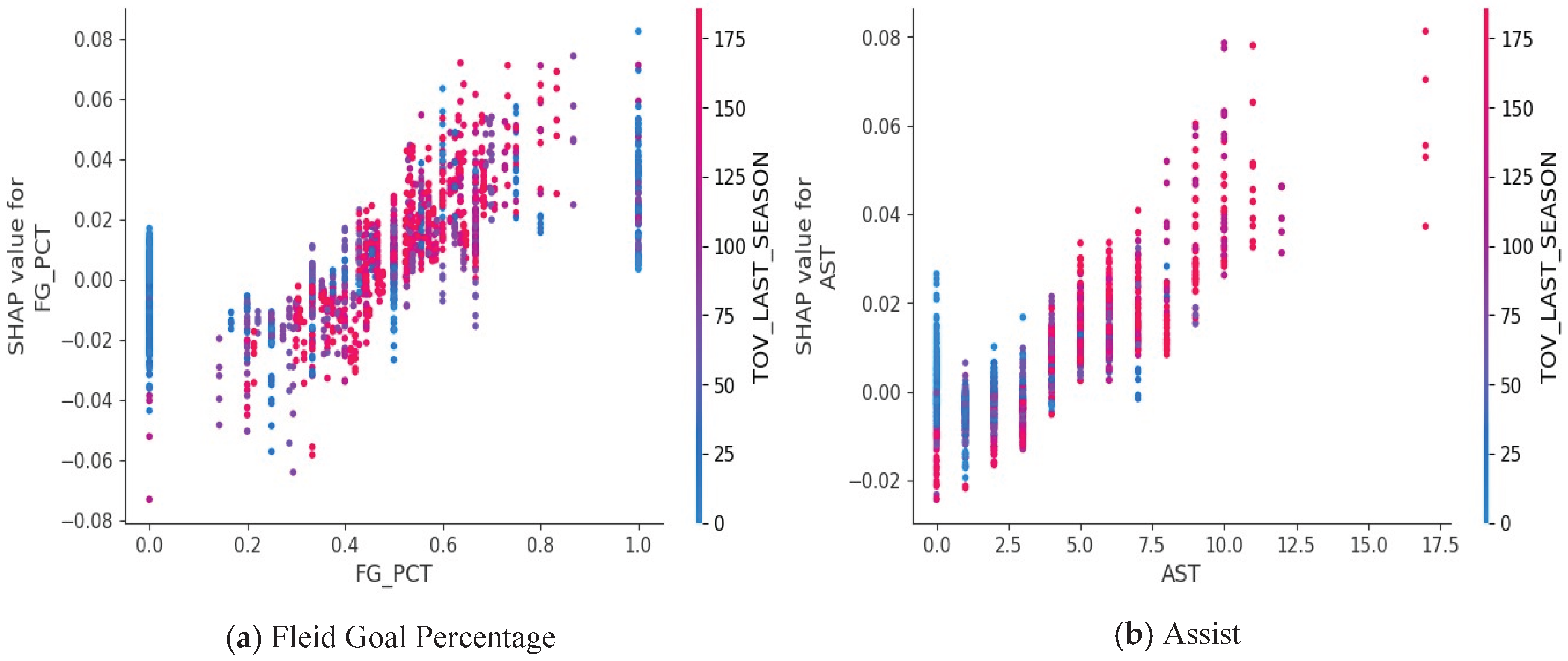
Figure 12.
SHAP Force Plot - OG Anunoby on October 25th, 2024.
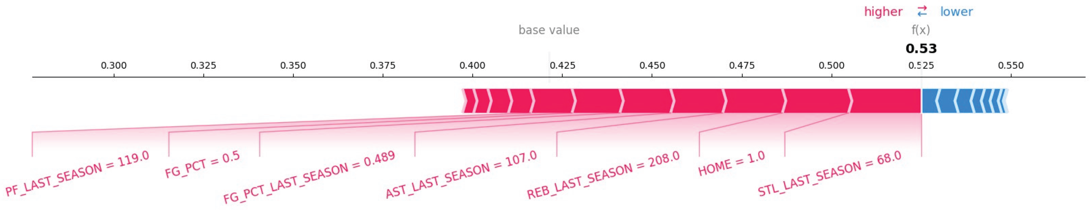
Figure 13.
SHAP Force Plot - OG Anunoby on November 10th, 2024.
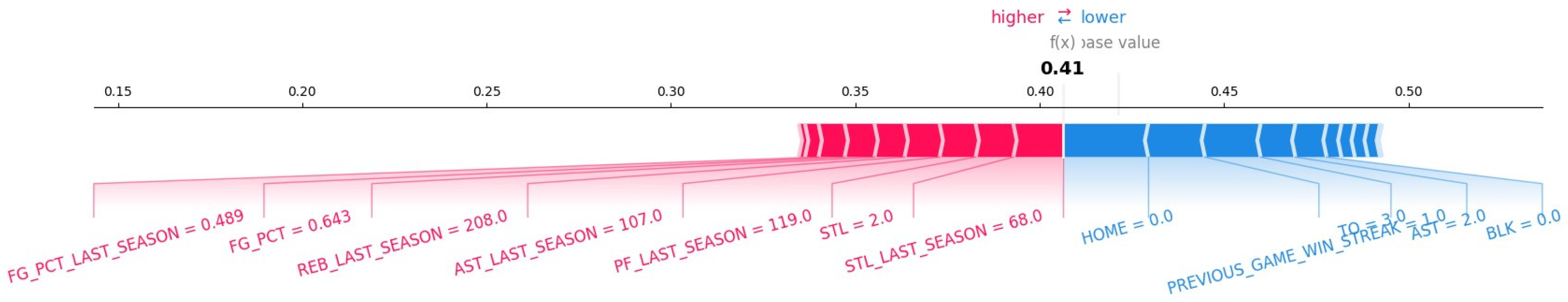
Figure 14.
SHAP Force Plot - OG Anunoby on Janunary 04, 2025.
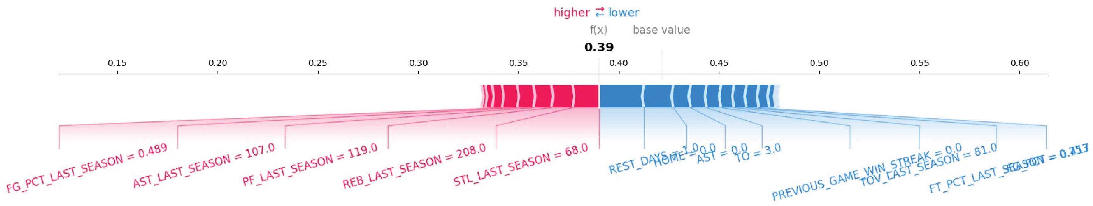
Table 1.
Base Model Performance.
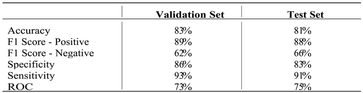 |
Table 2.
Stacked Confusion Matrix Across Validation and Test Set.
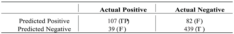 |
Table 3.
Performance metrics for different seeds.
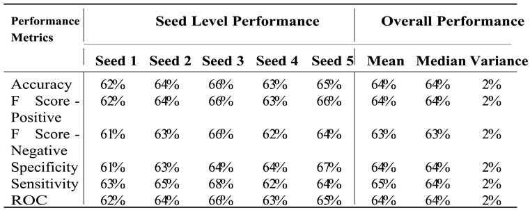 |
Table 4.
Stacked Confusion Matrix Across Five Seeds.
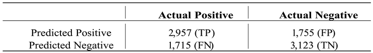 |
Table 5.
Performance metrics for different seeds.
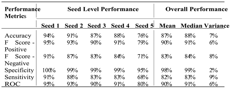 |
Table 6.
Stacked Confusion Matrix Across Five Seeds.
 |
Disclaimer/Publisher’s Note: The statements, opinions and data contained in all publications are solely those of the individual author(s) and contributor(s) and not of MDPI and/or the editor(s). MDPI and/or the editor(s) disclaim responsibility for any injury to people or property resulting from any ideas, methods, instructions or products referred to in the content. |
© 2025 by the authors. Licensee MDPI, Basel, Switzerland. This article is an open access article distributed under the terms and conditions of the Creative Commons Attribution (CC BY) license (http://creativecommons.org/licenses/by/4.0/).
Copyright: This open access article is published under a Creative Commons CC BY 4.0 license, which permit the free download, distribution, and reuse, provided that the author and preprint are cited in any reuse.


