Start Time End Time Integration (STETI): Analyzing Trends in Kidney Cancer Survival Time Data

Background/Objectives: Accurately estimating survival times for kidney cancer patients is critical for clinical decision-making, treatment evaluation, resource allocation other purposes. Yet data from relatively recent diagnosis cohorts presents an important difficulty: five, 10 or 20-year survival time averages are not available until 5, 10 or 20 years later, which may be in the future thus presenting a challenge to understand in the present. The proposed approach is shown for kidney cancer survival but could be applied to survival problems connected to survival for other types of cancer, other diseases, stage progression times, and similar problems in medicine and engineering in which there is a need to understand trends of improvement in survival. Methods: This study introduces a novel method for survival estimation that addresses limitations in traditional approaches by incorporating recent survival data often excluded due to incomplete longitudinal records. Leveraging data from the SEER database resource, the proposed approach integrates historical diagnosis year cohorts with more recent death year cohorts. This permits survival time trend analyses that account for both earlier and more recent improvements in treatment effectiveness. We used linear and exponential models to demonstrate the method's ability to predict survival trends using valuable data that would otherwise risk being ignored. Conclusions: Better survival estimates can better support personalized treatment planning, health care benchmarking, and research into cancer subtypes as well as other domains. This hybrid analytical approach paves the way to applications in oncology and beyond, and offers a robust method for quantifying and predicting the survival trends associate with therapeutic advancements.

Keywords:

survival

;

cancer

;

kidney

;

treatment

;

trend

;

STETI

Subject:

Public Health and Healthcare - Other

1. Background

1.1. Epidemiology and Significance of Kidney Cancer

Kidney cancer ranks among the ten most common cancers, representing over 3% of reported cancer cases globally (Ferlay et al. 2013; Wong et al. 2017). While advances in diagnostics and treatment have improved patient outcomes, the disease presents a complex epidemiological profile with diverse subtypes. Renal cell carcinoma (RCC) predominates and accounts for over 90% of these cases (Naik et al. 2024). While incidence of RCC is increasing (Padala et al. 2020), posing an important challenge, other types continue to present their own challenges in impact, diagnosis and treatment. Thus transitional cell carcinoma can occur in the kidneys (Tang et al. 2023), forming many of the non-RCC cases. Rarer subtypes are various. Examples include medullary renal carcinoma, highly treatable but only when correctly diagnosed. One case went viral with millions of views (Chubbyemu, 2021). Another rare subtype, Wilms tumor, can occur even before birth (Bechara et al. 2024). This underscores the heterogeneous nature of kidney cancer across age groups and histological subtypes, and the associated distinct diagnostic and therapeutic challenges.

1.2. Importance of Accurate Survival Estimation

Estimating survival time estimation contributes to kidney disease prognosis and guides patients, their families, and clinicians in making decisions about treatment and in future planning. Early work was reviewed by Kardaun (1991). Many patients want to know reliable survival estimates (Hagerty et al. 2005), as it empowers them to understand their journeys as well as helping them with emotional and financial preparedness. From a clinical perspective, survival predictions help in both designing personalized treatment protocols and optimizing follow-up schedules, thus improving overall care. At an institutional level, accurate survival data are needed for benchmarking treatment center performance (Wong et al. 2017) and thus helping to drive improvements in clinical practices.

Survival statistics and trends also play a significant role in research. They enable evaluating new treatments and can enable directing resources toward subtypes with the greatest potential for improvement. As treatments improve, traditional methods of survival analysis often fail to account for the trend in improvement, leading to outdated, potentially misleading underestimates. This limitation highlights the need for methodologies that use the available data in their analyses and adapt to the dynamics of improvement in cancer treatment.

Additionally, survival estimates can contribute to the healthcare system overall, such as in identifying cost-effective protocols for screening, treatment and follow up, and ultimately impacting healthcare policies, guidelines and costs.

1.3. Current Methods and Their Limitations

Existing survival estimation techniques have notable constraints. The Kaplan-Meier method is widely used in survival analysis. It estimates survival probability over time based on observed survival data, adjusting for patients that are lost to follow up and thus whose data is censored, hence incomplete. The Kaplan-Meier method, while effective at managing censored data, does not address trends of change in survival over time.

Cox proportional hazards models are widely used for analyzing covariate effects. They can analyze the relationship between survival time and predictor variables (age, stage, biomarkers, etc.) and provide estimates of hazard ratios which can facilitate calculating survival probabilities. While a time variable like diagnosis date can take the role of predictor variable, relatively recent diagnosis year cohorts present a challenge when complete data on their associated survival statistics is not yet available.

General approaches feature wide applicability. However, disease-specific methods can address characteristics of particular diseases. Such models often integrate multiple sources of evidence, thus providing a comparatively comprehensive evaluation. For instance, nomograms (Iasonos et al. 2008, Kou et al. 2021) are widely recognized for modeling specific cancers and are particularly useful in generating individualized predictions. They can calculate the probability of survival for a specified period, such as five years, by integrating multiple sources of evidence, including clinical, pathological, and molecular data, providing both estimates and error bounds. However, traditional nomograms, such as the ASSURE model for renal cell carcinoma (Correa et al. 2021), fail to incorporate recent advancements in therapeutic approaches like targeted therapies and immunotherapy. Thus nomograms can become dated in not accounting for improvement trends in treatment, leading to out-of-date forecasts for new diagnoses. This is a limitation in conditions like kidney cancer with significant trends of improvement in survival.

Survival prediction for kidney cancer, like other forms of cancer and other illnesses, has increasingly been explored using data mining and machine learning. These approaches leverage large datasets, derived from such sources as clinical records and cancer registries like SEER and others. SEER, the primary data source for this study, provides de-identified patient records, including the year of diagnosis and death, for a substantial portion of U.S. cancer cases. These records come from regions with rigorous reporting standards that help ensure high data quality, and encompass various cancer types.

Numerous techniques have emerged in this era of advanced data analysis. Random forests, for instance, have been extensively studied since even before the recent surge in neural network research (Shi et al. 2005) and continue to be investigated (Ranjan et al. 2022). Decision trees boast an even longer history, with their application predating the 21st century (François et al. 1999) and continued interest today (Souza-Silva et al. 2024). Neural network models, first proposed in 1958 (Rosenblatt), have in recent years surged to the forefront of artificial intelligence research and practice, and show significant potential for survival prediction in kidney and other cancers (Song et al. 2024). However, a key limitation of neural networks is their current inability to provide clear explanations for the results they generate. This challenge remains a critical focus of ongoing research (Yenduri et al. 2024). Addressing this issue will be essential for realizing the full potential of neural network-based predictions in kidney cancer and beyond.

Addressing the limitations of all these methods in relying on historical data that may no longer reflect the realities of current medical advancements is an ongoing need. Analyses should provide up-to-date forecasts that account for the trends in improved treatments, ensuring more accurate and relevant predictions.

1.4. The Problem and Its Resolution

If the problem was merely to identify the trend of improvement in survival over time and extrapolate from older data to present and future times, the solution would be simple. However, extrapolating from a fitted curve is only part 1 of the problem. Part 2 is to use newer data to assist. This is important because deriving improvement curve trajectories works better with more data and, because trend characteristics can vary over time (e.g. Mazzoleni et al. 2021; Muggeo 2008), newer data has even more value than older data. Yet new data, while available, is not complete enough to support strong conclusions about N-year survival until N years have elapsed, at which time the data will no longer be part of the new data category. For example, calculating metrics such as the 10-year cause-specific survival time requires using diagnoses from at least 10 years ago. This is a problem because the old data tells a different story than the new data, a story which is outdated and does not account well for the survival benefits accruing from the continuing stream of treatment improvements.

One approach to accounting for trends of survival improvement using the more challenging, newer data is the period analysis method. This was first adapted to the medical field by Brenner and Gefeller (1997). Their solution to using the newer data on those relatively recent diagnoses for which survival data is not yet available about some years in the time period of interest starting with that diagnosis year, is to impute data values for the not-yet existing data for those years (Brenner et al. 2004). Their imputation process is perhaps most easily grasped by a specific example; the reader may then generalize from that. Suppose we need survival numbers for each year of a 10-year period for diagnoses made in 2020, but the survival data available only goes through 2024. To impute the survival figure for 2025, use the 2024 figure for 2019 diagnoses. Similarly, to impute the 2026 survival for 2020 diagnoses use the 2024 number for 2018 diagnoses, for the 2027 survival use the 2024 number for 2017 diagnoses, and so on. However, some inaccuracy in the analysis remains because of the necessity to rely on imputing future data using historical data, a process which does not correct for the trend in treatment effectiveness in the imputed values. Such a correction could be estimated and used, but this would have to be an uncertain estimate. They report results that are clearly more accurate than those obtained from the base approach that simply ignores the recent data.

The method we describe here, end date based modeling, uses newer data from diagnosis years that mark the start of time periods that have not ended yet. To avoid imputing data that does not yet exist, the method shifts the focus from start (diagnosis) year cohorts to end year cohorts. A curve modeling the trend of survival time improvement is fitted to the end year based data. This curve is different, but arithmetically interconvertible with, the curve that would be fitted to diagnosis year based survival data if that data existed. Since the two curves are interconvertible, the end date based curve is then converted to a diagnosis date curve, which estimates survival from diagnosis date as desired.

This method can be used when the amount of data is not statistically large enough to conceal stochastic variation (noise), because it relies on regression to fit a smooth curve to data that might not be smooth. However, an unavoidable limitation is that it is possible for the quantity of data to be too small to do this reliably. Another inherent limitation is that fitting a curve means assuming the mathematical formula of the curve is a valid model of change in the effectiveness of treatment over time. Thus the method has certain limitations while providing distinctive advantages.

1.5. Objective of the Study

This study targets improved survival estimation with a novel method, end date based modeling, that combines trend analysis with the newer survival data (which reflects recent treatment outcomes), a data category that is challenging to leverage. To address this challenge, the method leverages death year cohorts instead of diagnosis year cohorts, a key step that enables using the relatively recent data that would otherwise be less usable. Applying this process to model trends of increase in survival times—driven by advancements in treatment—the method accounts for the dynamics of improvement in cancer care driven by the sequence of new treatments introduced over time. This approach reduces over-reliance on older datasets that can underestimate survival outcomes, providing results that are both more defensible and more optimistic.

The proposed method may be combined with more traditional diagnosis year based analyses, resulting in a hybrid framework that offers improved survival time estimation. This paper describes the development, implementation, and validation of this approach, highlighting its application to kidney cancer. However it is a general technique with applicability to other cancer types, subtypes and broader medical and other contexts. It is a framework for improved survival estimation when there is a trend of improvement in survival times.

2. Methods

End date based modeling starts with a model of improvement in survival time as treatment changes over time. Like the base approach, it is a model keyed to start (e.g. diagnosis) date as the independent variable and estimates survival time as a function of start date. However, unlike the base approach, it uses recent data not used in the base approach by employing the following process.

Steps of the end date based modeling process:

1): Specify a type of model for average survival time as a function of start year cohort. (We will assume start year is diagnosis year in the following, for ease of exposition, but it could be defined as a stage transition or any other plausible starting time point.)
2): Transform the function of diagnosis year algebraically into a function of death year.
3): Regress parameters in the function of death year to make it fit the data, which consists of an average survival time associated with each year of death cohort.
4): Algebraically transform the death year curve, with its parameters now specified, back into a diagnosis year curve.
5): Use the new diagnosis year curve for predictions and estimates as desired.

We next expand on each of these steps, providing the details that more fully explain how the method works.

2.1. Specify a Type of Model Estimating Survival Time as a Function of Diagnosis Year Cohort

Treatment extends patient survival time for most serious diseases. Because medicine, like other fields in which science and technology play roles, tends toward improvement over time, average survival times often increase over time. We might choose to model this increase as a linear (constant rate of) improvement over time, or instead as an exponential function of time, a logistic function or some other type of curve. Once fitted to historical survival data, different such models will often give similar predictions for present and near-future diagnoses since the fitting process will cause them all to attempt to follow the underlying trend behind the historical data.

An example appears in Figure 1. The 20-year average survival times for kidney cancer deaths are shown for the years 1992 through 2000. These averages are not available for recent diagnosis years because the average 20-year survival time is not available until 20 years after the diagnosis year. The exponential curve

{y = 3.0748 * 2}^{(x - 1992) / 93}

was fitted to the data points with the help of the Excel trend curve functionality. Note that the most recent data point is the average for year 2000 diagnoses, because data was only available up to 2020. Year 2000 is a long time ago to be the most recent diagnosis year cohort to analyze, especially as so many patients have been diagnosed more recently than that and have benefited from relatively recent advances in treatment technology. While a significant amount of survival data for individual patients is available for more recent diagnosis years, that data cannot be used to compute a 20-year average because not all of the needed full 20 years of data exist yet. Simply waiting 20 years until full data is available we will call the base approach, and presents a problem that calls out for solutions.

The method of this report addresses this problem by transforming the diagnosis year based analysis into a death year based analysis. Average survival times for death year cohorts are available for years that are more recent than 2000, up to 2020 for the data set. Thus, for example, the 2020 death year cohort includes diagnoses in 2001, 2002, …, 2020, which occurred after 2000 and thus could not be used in the base method. The transformation process is explained next.

2.2. Transform the Function of Diagnosis Year Algebraically into a Function of Death Year

As noted, a basic cohort analysis of survival time based on diagnosis year would involve following a cohort for perhaps a 5, 10 or 20 year period after diagnosis to be able to calculate a statistic like average survival time, or the percentage of patients surviving beyond 5, 10 or 20 years. Relatively new data is left unused. This makes the conclusions of the base method out of date for the many cancers for which advances in treatment over time lead to ever-improving outcomes. Even if a delay of 5 years was tolerable, the 20-year survival analysis results are likely to significantly underestimate the outcomes for current patients who have experienced treatment protocols adopted within the last 20 years. A model of survival as a function of diagnosis year needs to be converted into a function of death year, enabling using data records too recent to be used by the base method.

We start by deriving the death year based model for a linear diagnosis year model to illustrate the process, then adapt it to derive death year models for the the exponential and logistic diagnosis year models.

2.2.1. Deriving a Death Year Survival Model from a Linear Diagnosis Year Model

To begin, consider a typical general equation for a linear model (i.e. a straight line on an xy-plane):

y = m x + b

(1)

where y is the height of the line for any value of x on the horizontal axis, and b is the y-intercept, or height of the line where it crosses the y-axis (sometimes but not necessarily where x = 0). In the present context, we may restate the equation as

(Estimated survival time for a given diagnosis year)

= (Rate of improvement in survival time per year) * (Diagnosis year – 1990)

(2)

+ (Estimated survival time for diagnoses in 1990)

where the y-axis is placed so as to cross the x-axis at the year 1990 for convenience and because we do not wish to suggest that a model of cancer survival would be applicable in year 0, thousands of years ago. Eq. (2) modifies eq. (1) by specifying a particular application, and also by placing the y-axis so it crosses the x-axis at year 1990 instead of year 0.

Restating eq. (2) in more concise terms we get

survival(t_begin) =slope * (t_begin – 1990) + survival(1990)

(3)

and restating again we get

S_{t_{b}} (t_{b}) = M * (t_{b} - 1990) + S_{t_{b}} (1990)

(4)

indicating survival as a function of begin time,

S_{t_{b}} ()

, given the begin time parameter t_b, where M is the slope.

We wish to transform eq. (4), which is a model estimating survival time from time of diagnosis, into an equivalent model estimating survival time from time of death. This requires getting t_b and

S_{t_{b}} (t_{b})

out of eq. (4) and, instead, using t_e and

S_{t_{e}} (t_{e})

where t_e is an end time (time of death in the present context), and

S_{t_{e}}

( ) is a function estimating survival time from end time.

Observe that (end time) = (begin time) + (survival time), that is,

{t_{b} + S}_{t_{b}} (t_{b}) = t_{e} .

(5)

Similarly,

t_{e} - S_{t_{e}} (t_{e}) = t_{b} .

(6)

Therefore,

S_{t_{b}} (t_{b}) = S_{t_{e}} (t_{e}) .

(7)

Removing t_b and

S_{t_{b}} (t_{b})

from eq. (4) using eqs. (6) & (7),

S_{t_{e}} (t_{e}) = M (t_{e} - S_{t_{e}} (t_{e}) - 1990) + S_{t_{b}} (1990) = M t_{e} - M S_{t_{e}} (t_{e}) - 1990 M + S_{t_{b}} (1990)

Rearranging terms,

(M + 1) S_{t_{e}} (t_{e}) = M (t_{e} - 1990) + S_{t_{b}} (1990)

and so

S_{t_{e}} (t_{e}) = \frac{M}{M + 1} t_{e} + \frac{S_{t_{b}} (1990) - 1990 M}{M + 1}

(8)

Note that eq. (8) also happens to be linear, with survival time function

S_{t_{e}} (t_{e})

having slope M‍‍ ‍‍/ ‍(‍M‍ + ‍‍1‍)‍, and a value for survival time,

{[S}_{t_{b}} (1990) ‍ - ‍ ‍ 1990 M] / (M + 1)

, at which the curve crosses the y-axis, which is located at x = t_e = 1990.

2.2.2. Deriving a Death Year Survival Model from an Exponential Diagnosis Year Model

Transforming an exponential model of how survival time increases with advancing diagnosis year into a model of how it increases with advancing death year parallels the process for linear models.

One form of the general exponential equation is

y = c b^{x / d}

(9)

where c is the y-intercept or height of the curve (e.g. the predicted survival time) where it crosses the y-axis. This is where the exponent is zero, in this case where x = 0). The base b and time constant d in eq. (9) are redundant in that an exponential curve defined by setting b arbitrarily and then adjusting d as desired can alternatively be specified by setting d arbitrarily and adjusting b. We will use b = 2 because then increasing the exponent by 1 causes y to double. Thus b = 2 exposes the “doubling time” property frequently discussed in the technology foresight literature (e.g. Bias et al. 2014), with d being the doubling time.

For the present context we restate eq. (9) as

S_{t_{b}} (t_{b}) = S_{t_{b}} (2000) * 2^{(t_{b} - 2000) / d}

(10)

indicating survival as a function of begin time, with the y-axis shifted to cross the x-axis (here named the t_b-‍axis) at year 2000. We used 2000 here, and 1990 in the linear model description above, highlighting that the year chosen is arbitrary.

We wish to convert eq. (10), which is a model estimating survival time from time of diagnosis t_b, into an equivalent model estimating survival time from time of death. This requires replacing t_b and

S_{t_{b}} (t_{b})

in eq. (10) with t_e, the end time or time of death, and

S_{t_{e}} (t_{e})

where

S_{t_{e}}

is a function estimating survival time from end time.

As in the linear model scenario we need to replace t_b and

S_{t_{b}} (t_{b})

with t_e and

S_{t_{e}} (t_{e})

, using eqs. (6) & (7) again. We restate them here for convenience.

t_{e} - S_{t_{e}} (t_{e}) = t_{b}

(6)

S_{t_{b}} (t_{b}) = S_{t_{e}} (t_{e})

(7)

Applying eqs. (6) & (7) to eq. (10),

S_{t_{e}} (t_{e}) = S_{t_{b}} (2000) * 2^{(t_{e} - S_{t_{e}} (t_{e}) - 2000) / d}

(11)

We seek a model that predicts survival,

S_{t_{e}} ()

, from end date, t_e. However eq. (11) does not do that because

S_{t_{e}} ()

appears on both sides of the “=” sign and thus picking a value for t_e does not lead to eq. (11) producing a survival prediction

S_{t_{e}} (t_{e})

. We could consider solving eq. (11) for

S_{t_{e}} (t_{e})

but this is a non-trivial task. The closest thing to a close-form solution would be an equation that includes the Lambert W-function (also known as the omega function, the product logarithm, and the product log function). However, an alternative is to solve eq. (11) straightforwardly for end date t_e instead:

t_{e} = [S_{t_{e}} (t_{e}) + d {l o g}_{2} (S_{t_{e}} (t_{e}))] + k

with constant k defined by: k =

2000 - d {l o g}_{2} (S_{t_{b}} (2000))

(12)

Eq. (12), which is not exponential, readily supports finding t_e given a value for

S_{t_{e}} (t_{e})

, but what we need to do is the opposite and find survival time prediction

S_{t_{e}} (t_{e})

given t_e. This may be done by testing different values for

S_{t_{e}} (t_{e})

to find one that produces the desired value of t_e when plugged into eq. (12). A systematic approach to determining what values of

S_{t_{e}} (t_{e})

to test in order to converge as closely as needed to the value that leads the target value of t_e is provided by the well-known bisection method (Codesansar 2024).

2.2.3. Deriving a Death Year Survival Model from a Logistic Diagnosis Year Model

If a logistic model is chosen for how diagnosis year predicts survival time, transforming that into a model of how end year predicts survival time is similar to the process for the linear and exponential models.

The logistic equation in one of its general forms is

y = \frac{H}{1 + e^{- r (x - x_{m})}}

(13)

where H is the maximum height at which this type of S-curve levels off, r represents how fast the curve rises, which is greatest at the x-axis location x_m, where the height of the curve is H/2 (that is, the middle of the “S”), and e is typically Euler’s number although any other positive number could be used instead.

For the current domain we can restate eq. (13) as

S_{t_{b}} (t_{b}) = \frac{H}{1 + e^{- r (t_{b} - t_{H / 2})}}

(14)

which transforms into the survival time vs death year model, using the same process used above,

t_{e} = \frac{l n (s_{t_{e}} (t_{e}))}{r} - \frac{l n (H - s_{t_{e}} (t_{e}))}{r} + s_{t_{e}} (t_{e}) + t_{H / 2}

(15)

As for the exponential case, a bisection algorithm can be used with eq. (15) to get

s_{t_{e}} (t_{e})

from t_e.

2.3. Regress Death Year Curve to the Data

If treatment did not improve over time, the base method would be reasonable to consider for estimating average survival time because the older data it relies on would be substantially equivalent to newer data. However, since treatment of kidney cancer is improving, the base analysis is unreliable as it leaves out the most relevant data, which is the recent data.

Figure 2 illustrates the issue. It shows a schematic view comparing the data used by the new method presented here (red and purple) with the data used by the base method (blue and purple). Although the time period of each vertical red-and-purple bar matches the time period of a horizontal blue-and-purple bar, they differ in a critical way: Each horizontal bar represents a diagnosis year cohort, while each vertical bar describes a death year cohort. Thus a vertical bar contains cells with more recent data than the horizontal bar of the same time period, while a horizontal bar contains data cells with older data than the corresponding vertical bar. The white cells are not used in either analysis. They fall into three categorie: (i) those above the diagonal, which are empty because a diagnosis year cannot be after a death year; (ii) those in the lower right, which represent events that took longer than the 20-year observation periods, and (iii) the remainder, found in the empty area of the “V” between the blue and red regions, which are valid data yet nevertheless unused because those cells are both not in any 20-year cohort defined by a diagnosis year (because data was not yet available for the full 20 years of follow up as required) and also not in any 20-year cohort defined by a death year (because reliable data was not available for the full 20 preceding years as required). Note that the chart reflects that treatment technology is improving: Each red bar except one has a higher mean survival time than its corresponding blue bar (p<0.02).

The models derived earlier for linear, exponential and logistic trends of improvement in survival times have parameters that need to be specified in order to describe specific trend curves that could be designed to fit actual data and plotted on a graph. In linear modeling, eq. (4), we specify a slope parameter, M, and a y-axis intercept value

S_{t_{b}} (1990)

. These parameters describe linear models of how survival improves with increasing in diagnosis year. Models of linear survival improvement with increasing death year, eq. (8), have the same two parameters. Note however that, although eq. (8) is linear, its slope is not M, but

\frac{M}{M + 1}

, and its y-intercept is not

S_{t_{b}} (1990)

, but

\frac{S_{t_{b}} (1990) - 1990 M}{M + 1}

. Nevertheless, eq. (8) can be fully defined by specifying values for M and

S_{t_{b}} (1990)

, which are to be determined based on the data, including recent data not usable by diagnosis year models.

Exponential modeling parallels linear modeling in several ways. Here, the trend curve describing how survival improves with diagnosis year is defined exponentially by eq. (10) rather than linearly, and the parameters needing to be specified are the doubling time d, analogous to slope in the linear model and, like in the linear case, the y-axis intercept, which is

S_{t_{b}} (2000)

in eq. (10). Transforming eq. (10) into a curve of survival time increase vs death year gives eq. (12). This is not exponential and indeed a model of increasing survival vs death year cannot be exponential (Howell et al. 2019). Nevertheless, eq. (12) can be fully specified by defining values for the same parameters as in eq. (10), d and

S_{t_{b}} (2000)

Modeling using logistic curves follows the process for linear and exponential modeling. The trend curve for survival time vs diagnosis year, eq. (14), has parameters r and t_H_/2. Parameter r determines the maximum steepness or rate of increase of the S-curve, which occurs at the midpoint of the S where the variable t_b = the parameter t_H_/2 and the height of the curve is half of its maximum height H. The value of H is 20 years in Figure 1 since the maximum possible survival time for an observation period of 20 years is 20 years. Parameter t_H_/2 is the time at which the height reaches H/2, and adjusting this parameter has the effect of shifting the S-curve left or right. Transformed into a model of survival time vs death year, we get eq. (15) which is not a logistic curve but has the same two parameters, whose values can be defined based on the data.

The linear, exponential and logistic models all have a rate parameter (respectively slope, doubling time and maximum steepness). The models also have a y-intercept parameter (respectively and necessarily partly arbitrarily, they are the curve height for given year 1990, the curve height for given year 2000, and the year for given height H/2). These two parameters are discussed individually in the following two subsections.

2.3.1. Determining the y-Intercept Parameter

Recall that death date based models can leverage recent data that diagnosis date based models cannot. Conversely, diagnosis date based models can leverage historical data that death date based models cannot. Thus diagnosis date modeling is valuable for analyzing early data for the same reason death date modeling is valuable for analyzing recent data. Since diagnosis year modeling is well-known and established, we will use it for data analysis up to the most recent year t_r for which it is usable. Years more recent than that require death year modeling. Year t_r and its survival time estimate provided by diagnosis year based modeling also provides a starting point for the trajectory of a survival curve predicted by a death year based model. For instance, in Figure 1, this point is at year 2000, the time of the last survival time data point available to diagnosis year based models, and the height of the point is 3.262, the height of the curve for year 2000. We therefore set

S_{t_{b}} (2000) = 3.262

in eq. (12) for exponential modeling as in Figure 1.

A few questions about this method are considered next.

FAQ

Q: What if we need to set

S_{t_{b}} (2000)

but wish to use linear modeling, for which eq. (4) contains the term

S_{t_{b}} (1990)

A: A numerical value for

S_{t_{b}} (1990)

is needed in the linear model of eq. (4), but if one wishes to instead specify a value for

S_{t_{b}} (2000)

, eq. (4) can be restated equivalently as eq. (16).

S_{t_{b}} (t_{b}) = M * (t_{b} - 1990) + S_{t_{b}} (1990)

(4)

S_{t_{b}} (t_{b}) = M * (t_{b} - 2000) + S_{t_{b}} (2000)

(16)

The same argument applies to exponential modeling.

Q: Why not optimize the fit of the death year curve to the data by regressing it on both the y-intercept and steepness parameters, instead of setting the y-intercept and regressing just the steepness parameter?

A: This is a modeling decision. An argument for setting the y-intercept using the diagnosis year analysis is that diagnosis year analysis uses more of the historical data (blue cells in Figure 2), thus reducing the stochastic noise problem that bedevils smaller data sets. An argument for using only death year data to determine both the y-intercept and steepness parameters is that newer data may better reflect the current underlying trend if it has changed over time. All too often, modeling decisions are judgment calls that depend on problem specifics and the modeler’s experience.

Q: How can a true shift in models be distinguished from shifts arising due to such factors as noise in the data, apparently random fluctuations in the model parameters over time, and discontinuous changes due to discontinuous shifts in treatment methods where these changes may or may not counterbalance each other over time?

A: This is a difficult question that surrounds the problem of trend analysis. See e.g. Farmer and Lafond (2016).

Q: Shouldn’t multiple modeling approaches be used instead of focusing on just one model? Then their results could be combined to provide an average prediction and/or a range or set of predictions.

A: Yes, as for example the spaghetti diagrams used for hurricane path prediction, showing the different paths predicted by the numerous different weather simulation models (Track the Tropics 2024).

2.3.2. Determine the Steepness Parameter

Once the y-intercept parameter has been specified as just described, the remaining parameter to determine is the steepness. To find the steepness, regress the steepness parameter in

S_{t_{e}} (t_{e})

, the function that predicts survival time from end date t_e (for “end time”), to the data points that associate survival times with death years. For the example of Figure 1 above, that means using eq. (12) as follows.

Set the value of $S_{t_{b}} (2000)$ in eq. (12) using the equation shown in Figure 1 to find its prediction for survival in year 2000. Solving $S_{t_{b}} (2000) = 3.0748 e^{0.0074 * (x - 1992)}$ yields $S_{t_{b}} (2000) = 3.2623$ .
Substitute $S_{t_{b}} (2000)$ in eq. (12) with 3.2623 to get

$t_{e} = [S_{t_{e}} (t_{e}) + d {* l o g}_{2} (S_{t_{e}} (t_{e}))] + 2000 - d * {l o g}_{2} (3.262324) .$

(17)

Regress d in eq. (17) to the death date vs survival time data to find the value for d that results in the equation fitting the data as well as possible. In doing so, for each candidate value of d, we need to compute $S_{t_{e}} (t_{e})$ for each value of t_e that we have data for. This will enable comparing the model curve $S_{t_{e}} (t_{e})$ with each data item so that the fit of the curve can be calculated for that d. This regression process will identify the d with the best fit to the data. Calculating $S_{t_{e}} (t_{e})$ was explained in the earlier discussion of eq. (12). The result of this process was d = 106 (for full details see Berleant 2024).

Survival time as a function of death year,

S_{t_{e}} (t_{e})

, has now been regressed based on Figure 1 and the red-and-purple data of Figure 2. Next we transform

S_{t_{e}} (t_{e})

back into survival time as a function of diagnosis year. This will update the curve of Figure 1 to account for the red data of Figure 2.

2.4. Transform the Death Year Curve Back into an Updated Diagnosis Year Curve

The diagnosis year curve is readily obtained from the death year curve. Both curves have the same y-intercept and steepness parameters. With those parameter values now determined by the regression computation, their values are plugged back into the diagnosis year function to get a revised

S_{t_{b}} (t_{b})

Continuing the example accordingly, we have (i) the y-intercept parameter

S_{t_{b}} (2000) = 3.2623

, and (ii) the doubling time parameter d = 106. Plugging them into eq. (10) gives

S_{t_{b}} (t_{b}) = 3.26232411 * 2^{(t_{b} - 2000) / 106}

(18)

which is graphed in bold in Figure 3. The new curve was developed under the assumption that the curve of the base method (also shown in Figure 3), is valid up to year 2000. Thus we graph the new curve starting from year 2000.

Understanding the discrepancy between base method and new method. Several interesting factors contribute to the differences between the two models’ predictions.

Noisy data. Random and seemingly random fluctuations may affect the data due to stochastic, temporary, unmeasured, and/or unmodeled factors. For instance, external influences such as pandemics, economic cycles, etc., can introduce variability that the model does not accounted for. This unpredictability highlights the limits of modeling complex phenomena, because models inherently simplify an endlessly complex reality.
Changes in model parameters over time. Changes in the reality being modeled can occur, changing the relationships among model variables. In such cases, a single model might not effectively represent the dynamics over an extended period. A regression model may then need to be piecewise, modeling different parts of the time period differently. The Chow test is commonly used to handle such break points. Other tests, such as the CUSUM test (Cumulative Sum of Residuals) and the Bai-Perron test, can also be useful in dealing with model shifts over time. However, the application of such methods is unclear in cases like the 20-year kidney and renal cancer survival example, where the base analysis approach is used on earlier data while more recent data uses the new approach.
Short-term variation with reversion to the mean. Sometimes shifts in a trajectory over time can be short term variations within the context of a more consistent long term trend.
For example, a model of long term economic growth might need to accommodate shorter term recessions within an overarching trend rather than as evidence against such a trend. Similarly, models of technological advancement may show long term trends which are composed of short term segments caused by a specific changes in the technology (e.g. Park 2017). Thus, it is important to consider that changes in a trajectory may be merely temporary excursions from the longer term trend rather than fundamental shifts.
Spaghetti diagrams, ensembles and cones of uncertainty. It would be convenient if there were a single best model, but an ensemble combining multiple models may more effectively represent the spectrum of possible outcomes. Spaghetti diagrams exemplify this approach by providing a visual representation of the outcome paths. This approach is familiar for example in meteorology, where spaghetti models are widely used to represent the different possible tracks of hurricanes. This technique is commonly used for example in meteorology to incorporate uncertainty in forecasts of hurricane trajectories (Belles, 2024).

Ensemble modeling also includes processing multiple output possibilities in other ways as well, such as averaging them to estimate a single “best guess” trajectory, or providing probabilities of different outcomes. Figure 3 depicts a simple 2-trajectory spaghetti diagram, the trajectories forming a small ensemble used to depict a cone of uncertainty.

3. Results

Using the new approach, we analyzed kidney and renal cancer data from SEER 12 (National Cancer Institute, 2025), querying for data on patients who were diagnosed and passed away from kidney and renal pelvis cancer throughout the years 1992 to 2020. Average survival times were calculated for yearly diagnosis cohorts using the base method and for yearly death cohorts using the new method), over three periods of observation: 5, 10, and 20 years. Since each cohort required survival data for a full 5, 10, or 20 years to be analyzed, this constrained which cohorts were usable. Figure 2 exemplifies the details using the 20-year case. For each time period both the exponential and linear models were applied. The results are given next.

3.1. Average Survival Times over 5-Year Observation Periods

Five-year survival trend analyses are shown in Figure 4. The data obtained covered years 1992 through 2020. Since the curves shown extend to the year 2030, they are necessarily extrapolations after 2020. In the graph, y is the vertical axis so a height in the graph defines a value for y and represents survival time in years. The x axis is the horizontal axis and gives diagnosis year values for locations within the graph. Since each data point represents an average for a diagnosis year cohort, they only go up to 2015, since for diagnosis years 2016 and beyond, survival data for the following 5 years, required to calculate the average 5-year survival time, is not available.

Key:

Diagnosis year cohort average survival time

____: Linear model based on diagnosis year cohort data

_ _ _: Linear model based on both diagnosis and death year cohort data

____: Exponential model based on diagnosis year cohort data

_ _ _: Exponential model based on both diagnosis and death year cohort data

3.2. Average Survival Times over 10-Year Observation Periods

Ten-year survival trend analyses are shown in Figure 5. Since each data point represents an average for a diagnosis year cohort, they only go up to 2010, since for diagnosis years 2011 and beyond, survival data for the following 10 years, required to calculate the average 10-year survival time, is not available.

Key (same as for Figure 4):

Diagnosis year cohort average survival time

____: Linear model based on diagnosis year cohort data

_ _ _: Linear model based on both diagnosis and death year cohort data

____: Exponential model based on diagnosis year cohort data

_ _ _: Exponential model based on both diagnosis and death year cohort data

3.3. Average Survival Times over 20-Year Observation Periods

Twenty-year survival trend analyses are shown in Figure 6. Since each data point represents an average for a diagnosis year cohort, they only go up to 2000, since for diagnosis years 2001 and beyond, survival data for the following 20 years, required to calculate the average 20-year survival time, is not available.

Key (same as for Figure 4):

Diagnosis year cohort average survival time

____: Linear model based on diagnosis year cohort data

_ _ _: Linear model based on both diagnosis and death year cohort data

____: Exponential model based on diagnosis year cohort data

_ _ _: Exponential model based on both diagnosis and death year cohort data

3.4. Average Survival Times over All Observation Periods

The results of Figs. 4, 5 & 6 show qualitative commonalities for all three survival time observation periods. Clearly, survival time is benefiting from a trend of improvement. Obviously then, using survival estimates from bygone years underestimates survival for newly diagnosed renal carcinoma patients. Equally clearly, trend estimates that use the new method to leverage both older and more recent data (dashed curves) differ noticeably from trend estimates that rely only on the older data and consequently ignore the more recent data. This shows that in addition to accounting for the fact of improvement in survival over time, how trends of improvement are determined had a clear effect on quantitative estimates of survival time.

4. Discussion

4.1. Long-Term Trends in Treatment Are Composed of Multiple Short-Term Advances

Any long term history of advancement in a technological domain will contain specific advances that were discovered, diffused into wider use, and eventually ceased to contribute directly to further advancement by achieving full market penetration and/or becoming replaced by newer and better advances. These individual advances each generally have logistic or other S-curve short-term characteristics that become components of the overarching long-term advancement process (Kucharavy and De Guio 2011).

Considering kidney and renal cancer treatment as a problem and a technological domain in which overall advancement results from multiple specific advances, a list of relatively recent specific drug advances is shown in Table 1.

With the long-term trajectory of treatment improvement structured as a combination of the effects of specific short-term improvements, it is natural to propose that the long-term trajectory would have a stepwise appearance, with steps corresponding to individual improvements in treatment. However, as a putative cause of unevenness in the long-term trajectory, this does not work, because an improvement generally exerts an influence that rises, plateaus, and perhaps then falls if it is replaced by another improvement (Figure 7). The effects of each improvement thus become smeared with the effects of others.

4.2. Comparing Methods and Models

Comparison across results show differences of multiple types. One is the consistent—and welcome—finding that survival times are increasing over time. Another noteworthy finding is that the trajectories of the curves for survival time increases vary depending on whether they are derived from older, diagnosis cohort data only, or from newer, death cohort data in addition. A third outcome is the varying predictions of curves for linear compared to exponential models.

Survival times are increasing. A striking aspect of the results is that all analyses whether for linear or exponential models, base analysis or the new method, and for all time periods tested, a trajectory of increasing survival time is apparent. Presumably this is due to improving treatment. As a result, failing to account for the history of repeated improvements in treatment effectiveness will tend to lead to underestimating survival times for current patients. Thus incorporating trend analysis in survival estimates is important, highlighting the need for good trend analyses and thus good trend analysis techniques.

The new method addresses shortcomings of the base method. The results clearly show that the new method and the base method produce different results. Since the new method is supported by relatively newer data that is not available to the base method, changes in the rate of increase in survival time will be reflected in different steepnesses for the trajectory curves of these methods. Indeed, it is frequent, though with notable exceptions like the search for laws of history (Turchin 2016), for timely data to better support understanding current conditions than out-of-date data. However this is not the only potential cause of different trajectories. More data tends to reduce the impact of noise within a data set. The new method uses more data than the base method, in that it uses the base method to help determine the trajectory (by setting the y-intercept parameter), while also using additional recent data (to set the steepness parameter). An example is Figure 6, which shows a rather small cloud of data points with considerable spread, suggesting that the trajectory produced by the base method might be unreliable. However, the new method lends circumstantial support to the base method trajectory, while revising it, by providing a new trajectory that is relatively similar.

The difference in results across the two methods is not dramatic. The difference between the trajectories of the base method vs the new method for near-term estimates is relatively modest. For example it is readily apparent from Figs. 4 – 6 that differences in survival time predictions across the two methods, for diagnosis year 2025, range from a few weeks to a few months. This relative concordance of predictions helps validate the foundations of both methods, without overshadowing the methodological advantages of the new method: using more and newer data is better, and survival time is important so even modest differences are worth getting right.

Linear vs exponential models. A comparison between the linear and exponential models whose trajectories are shown in Figs. 4 – 6 reveals that these models produce similar trajectories, particularly in shorter time frames. Theoretically, survival times must eventually approach an upper limit defined by the observation period (5, 10, or 20 years), suggesting that an S-curve model might ultimately prove most appropriate for very long-term projections. Exponential and other curved phenomena, when viewed over a sufficiently short time span, become effectively linear. A logistic S-curve, in turn, has an initial portion that is effectively exponential. Regardless, the linear and exponential models coincide fairly in the experiments herein, though the discrepancies increase as they are extrapolated into the future. This concordance is unsurprising as both are tuned by y-intercept and steepness to fit the same data. Unless the primary interest is in long-term extrapolation, an inherently speculative endeavor anway, the question of what is the “right” model is not of overriding importance. Instead, by considering both simultaneously, they can provide input to an uncertainty quantification analysis using a spaghetti diagram and cone of uncertainty.

Ensembles, spaghetti diagrams and cones of uncertainty. Each set of results in Figs. 4 – 6 shows multiple trajectories, forming an ensemble of curves that led to spaghetti diagrams with diverging tendencies forming a cone of uncertainty. The paths forming the spaghetti diagram and its enclosing cone of uncertainty communicates uncertainty that increases over time using a range of representative outcomes. Rather than viewing different results from different methods as representing an unresolved conflict, it may instead be useful to acknowledge that all models are imperfect representations of reality. This motivates running multiple models, as we have done here, as an ensemble. The differing predictions can then be usefully interpreted as revealing the inherent uncertainty in the prediction analysis. This perspective highlights the power of ensemble modeling to convey uncertainty and offer a richer representation of potential survival trajectories.

By integrating the outputs of multiple models, the ensemble framework leverages the strengths of diverse methodologies, enhancing understanding of the uncertainties in predictions. The cone of uncertainty also serves as a powerful reminder of the limits of predictability in the behavior of complex systems.

4.3. Why Identify Trends of Improvement in Kidney Cancer Treatment?

The findings presented here have implications for both clinical practice and research methodology. For clinicians, the results suggest using survival estimates that incorporate the effects of recent treatment advances to obtain more reliable estimates. For researchers, trend findings that incorporate newer data and are thus up-to-date more strongly suggest the likely magnitude of benefits of future treatments, providing expectations that can help drive the discoveries required to achieve those benefits (Mulay 2022).

5. Conclusions

The work presented here provides a starting point for addressing its limitations as well as building on it with a range of applications and extensions.

First, although the new method incorporates data not used by the base method, there is other data not used by either method. The white cells in Figure 2 between the arms of the red and blue V are each associated with a diagnosis year, death year, and number of patients, providing valid data not used in either the blue-and-purple base analysis or the red-and-purple new analysis. Further research might give a way to use these cells so as not to “waste” data.

Second, future work is needed to apply this methodology to other cancer types and subtypes. A broad cancer category like kidney cancer includes subtypes with differences in their treatment protocols and survival expectations, as well as their rate of increase in survival time due to improvements in treatment. Such subtypes could be defined genetically, for example, and this is expected to become more prevalent as genetic sequencing and profiling advances. The approach can be applied to other categories of cancers, such as myeloma and lung cancer (Chaduka 2024). It can also be applied to subtypes of these and other cancers for which treatments are improving. We are currently investigating myeloma subtypes and have obtained preliminary results for the CD-2 genetic subtype. Similarly, survival after diagnosis is generalizable to survival after transition to a particular stage of cancer, to time in a particular stage, and so on. Other serious disease besides cancer could be analyzed similarly. The method also holds promise for application in non-medical domains such as engineering, where manufactured artifacts may exhibit increases in product life as their associated technologies advances (e.g. Howell et al. 2019).

Third, while this study explored exponential and linear models of increasing survival times, alternative models, such as logistic or other sigmoidal (S-curve) models, also warrant investigation. Moreover, the underlying drivers that are being modeled may shift over time, leading to the need for alternative modeling that can capture such shifts. A more flexible and diverse modeling toolbox would permit a richer characterization of long-term dynamics.

Fourth, the new approach needs to be modified for application to Kaplan-Meier survival functions. When survival metrics improve over time, these functions change accordingly. If the approach could be adapted to this context, sets of K-M survival functions showing the survival profiles of cohorts associated with different time periods could be analyzed to quantitatively determine how metrics like median survival time or survival time at specific percentiles evolve over time.

Finally, quantifying uncertainty in the modeling process using ensembles, spaghetti diagrams and cones of uncertainty can certainly be developed beyond the hints of this methodology given herein. Confidence intervals would also be useful. These techniques would provide better visualizations of the variability and uncertainty in modeling, leading to fuller pictures of what can be concluded about survival trends and their extrapolations.

Together, these directions highlight the potential to refine and extend the methodology, enhancing its applicability and impact across medical and other domains.

5.1. Improving Survival Analysis: Concluding Note

This study focuses on the critical problem of adapting survival estimation methodologies to account for the dynamic improvement over time in treatment outcomes. By introducing an end date-based modeling approach, we provide a framework that not only addresses existing limitations in leveraging recent survival data but also paves the way for more accurate and optimistic survival predictions. We demonstrated the method on kidney cancer, yet its applicability extends beyond that to include other cancer types, cancer subtypes, other diseases and even non-medical domains. This approach represents a significant step forward in survival analysis, able to help inform patients, their doctors, research on treatment advances and research policy.

Author Contributions

TC performed the data analyses, generated figures and interpreted results. DB coordinated the project and developed the analysis software and the STETI method. MB assisted with study design and coordination. PT contributed insights toward the development of the method. SMT contributed oncology domain knowledge. All authors read and approved the final manuscript.

Funding

This work was supported in part by NIH subaward 54077-CRG of 5P20GM103429-23, and by the National Science Foundation under award OIA-1946391.

Institutional Review Board Statement

This study was conducted as approved by the Institutional Review Board of the University of Arkansas at Little Rock (protocol #24-001-R3, Feb. 5, 2024).

Informed Consent Statement

Patient consent was waived due to meeting the IRB’s criteria for protection of human participants without patient consent.

Data Availability Statement

Data used in this study was obtained from SEER (https://seer.cancer.gov/registries/terms.html). It was tabulated for use in the research into tables provided in the appendices of Chaduka (2024). Software for providing the results illustrated in Figs. 4, 5 & 6 is available as web pages containing embedded JavaScript for making the calculations upon request to the corresponding author.

Acknowledgments

During the preparation of this manuscript, the authors used generative AI for the purposes of polishing selected passages. The authors have reviewed and edited the output and take full responsibility for the content of this publication.

Conflicts of Interest

The authors declare no conflicts of interest.

Abbreviations

The following abbreviations are used in this manuscript:

SEER Surveillance, Epidemiology, and End Results Program of the US National Cancer Institute

References

Bechara, E, Saadé, C, Geagea, C, Charouf, D, and Abou Jaoude, P. Fetal Wilm’s tumor detection preceding the development of isolated lateralized overgrowth of the limb: a case report and review of literature. Frontiers in Pediatrics 2024, 12. [Google Scholar]
Belles, J. Hurricane spaghetti models, The Weather Company, August 20, 2024, https://weather.com/science/weather-explainers/news/2024-08-20-hurricane-spaghetti-models-track-like-pros.
Berleant, D. Data from SEER Nov 2022 Sub (1992-2020) Database - 20 Year Cause-Specific Survival Time of Kidney & Renal Cancer Patients That Died in Years 2012-2020, Exponential Model, T0=2000, lifeAtT0 = 3.2623, Sept. 19, 2024, https://dberleant.github.io/TCresearch/kidney20yearSurvivalT0is3point262.html.
Bias, R. , Lewis, C., & Gillan, D. The Tortoise and the (Soft)ware: Moore’s Law, Amdahl’s Law, and Performance Trends for Human-Machine Systems. Journal of Usability Studies 2014, 9, 129–151. [Google Scholar]
Brenner, H. , & Gefeller, O. Deriving more up-todate estimates of long-term patient survival. Journal of Clinical Epidemiology 1997, 50, 211–216. [Google Scholar]
Brenner, H. , Gefeller, O. and Hakulinen, T. Period analysis for ‘up-to-date’ cancer survival data: theory, empirical evaluation, computational realisation and applications. European Journal of Cancer 2004, 40, 326–335, https://www.sciencedirect.com/science/article/pii/S0959804903009237. [Google Scholar] [CrossRef]
Chaduka, T. M. Method for Measuring the Rate of Improvement in Survival Times of Cancer Patients, dissertation, University of Arkansas at Little Rock, Dec. 2024, https://dberleant.github.io/papers/tchadukadissertation.pdf.
Chubbyemu channel. A Man Found Blood In His Urine. This Is What Was Growing In His Kidneys, 2021, youtube.com, https://www.youtube.com/watch?v=3E75UvmY9GA.
Codesansar. Bisection method algorithm (step wise), downloaded 2024, https://www.codesansar.com/numerical-methods/bisection-method-algorithm.htm.
Correa, A. F. , Jegede, O. A., Haas, N. B., Flaherty, K. T., Pins, M. R., Adeniran, A., Messing, E. M., Manola, J., Wood, C. G., Kane, C. J., Jewett, M. A. S., Dutcher, J. P., DiPaola, R. S., Carducci, M. A., & Uzzo, R. G. Predicting disease recurrence, early progression, and overall survival following surgical resection for high-risk localized and locally advanced renal cell carcinoma. European Urology 2021, 80, 20–31. [Google Scholar] [CrossRef] [PubMed]
Drugs.com. Zortress FDA Approval History, 2010, https://www.drugs.com/history/zortress.html.
Drugs.com. FDA Approves Merck’s Welireg (belzutifan) for the Treatment of Patients With Advanced Renal Cell Carcinoma (RCC) Following a PD-1 or PD-L1 Inhibitor and a VEGF-TKI, 2023, https://www.drugs.com/newdrugs/fda-approves-merck-s-welireg-belzutifan-patients-advanced-renal-cell-carcinoma-rcc-following-pd-1-6177.html.
Farmer, J. D. and Lafond, F. How predictable is technological progress? Research Policy 2016, 45, 647–665. [Google Scholar] [CrossRef]
Ferlay, J. , Soerjomataram, I., Ervik, M., et al. GLOBOCAN 2012v1.0, Cancer Incidence and Mortality Worldwide. IARC Cancer Base No. 11, Lyon, France: International Agency for Research on Cancer, 2013.
François, C. , Decaestecker, C., de Lathouwer, O., Moreno, C., Peltier, A., Roumeguere, T., Danguy, A., Pasteels, J.-L., Wespes, E., Salmon, I., van Velthoven, R., & Kiss, R. Improving the prognostic value of histopathological grading and clinical staging in renal cell carcinomas by means of computer-assisted microscopy. Journal of Pathology 1999, 187, 313–320. [Google Scholar]
Google Scholar. Articles found using the search query intitle:Sunitinib intitle:renal and counted by year using the “Custom range...” link, downloaded 2024, http://scholar.google.com.
Hagerty, R. G. , Butow, P. N., Ellis, P. M., Dimitry, S., & Tattersall, M. H. N. Communicating prognosis in cancer care: a systematic review of the literature. Annals of oncology 2005, 16, 1005–1053. [Google Scholar] [CrossRef]
Howell, M. , Kodali, V., Segall, R., Aboudja, H. and Berleant, D. Moore’s law and space exploration: new insights and next steps. Journal of the Arkansas Academy of Science 2019, 73, 13–17, https://scholarworks.uark.edu/jaas/vol73/iss1/6. [Google Scholar] [CrossRef]
Iasonos, A. , Schrag, D. , Raj, G. V., & Panageas, K. S. How to build and interpret a nomogram for cancer prognosis. Journal of Clinical Oncology 2008, 26, 1364–1370. [Google Scholar] [CrossRef]
Kardaun, O. J. W. F. Kidney-survival analysis of IgA-nephropathy patients: A case study. In C. R. Rao & R. Chakraborty (Eds.), Handbook of Statistics (Vol. 8, pp. 407–459). Elsevier Science Publishers B.V., 1991. [CrossRef]
Kou, F. R. , Zhang, Y. Z., & Xu, W. R. Prognostic nomograms for predicting overall survival and cause-specific survival of signet ring cell carcinoma in colorectal cancer patients. World Journal of Clinical Cases 2021, 9, 2503–2518. [Google Scholar] [CrossRef] [PubMed]
Kucharavy, D. and De Guio, R. Logistic substitution model and technological forecasting. Procedia Engineering 2011, 9, 402–416. [Google Scholar] [CrossRef]
Lane, Y. F. FDA Approves Pembrolizumab plus Axitinib for Advanced Renal-Cell Carcinoma. The Oncology Pharmacist, 2019, https://theoncologypharmacist.com/web-exclusives/17731:fda-approves-pembrolizumab-plus-axitinib-for-advanced-renal-cell-carcinoma.
Mazzoleni, M. , Breschi, V., & Formentin, S. Piecewise nonlinear regression with data augmentation. IFAC-PapersOnLine 2021, 54, 421–426, https://www.sciencedirect.com/science/article/pii/S2405896321011708. [Google Scholar]
Muggeo, V. M. Segmented: an R package to fit regression models with broken-line relationships. R news 2008, 8, 20–25, https://journal.r-project.org/articles/RN-2008-004. [Google Scholar]
Mulay, A. Sustaining Moore’s Law: Uncertainty Leading to a Certainty of IoT Revolution, Springer Nature Switzerland AG, 2022.
Naik, P. , Dudipala H., Chen Y.-W., Rose B., Bagrodia A., McKay R. R. The incidence, pathogenesis, and management of non-clear cell renal cell carcinoma. Therapeutic Advances in Urology 2024, 16. [Google Scholar] [CrossRef]
National Cancer Institute. Registry Groupings in SEER Data and Statistics. Downloaded Jan. 2025, https://seer.cancer.gov/registries/terms.html.
Padala S., A. , Barsouk A., Thandra K. C., Saginala K., Mohammed A., Vakiti A., Rawla P., Barsouk A. Epidemiology of Renal Cell Carcinoma. World J Oncol. 2020, 11, 79–87. [Google Scholar] [CrossRef] [PubMed] [PubMed Central]
Park, C. Definition and measurement of S-curve based technological discontinuity: Case of technological substitution of logic semiconductors. Journal of the Korea Academia-Industrial Cooperation Society 2017, 18, 102–108. [Google Scholar] [CrossRef]
Ranjan, M. Shukla, A., Soni, K., Varma, S., Kuliha, M., & Singh, U. Cancer prediction using random forest and deep learning techniques. In 2022 IEEE 11th International Conference on Communication Systems and Network Technologies (CSNT), pp. 227–231, 2022, IEEE. [CrossRef]
Rosenblatt, F. The perceptron: A probabilistic model for information storage and organization in the brain. Psychological Review 1958, 65, 386–408. [Google Scholar] [CrossRef]
Shi, T. , Seligson, D., Belldegrun, A. S., Palotie, A., & Horvath, S. Tumor classification by tissue microarray profiling: Random forest clustering applied to renal cell carcinoma. Modern Pathology 2005, 18, 547–557. [Google Scholar] [CrossRef]
Song, A. H. Chen, R. J., Jaume, G., Vaidya, A. J., Baras, A., & Mahmood, F. Multimodal prototyping for cancer survival prediction. In Proceedings of the Forty-first International Conference on Machine Learning, 2024. https://openreview.net/forum?id=3MfvxH3Gia.
Souza-Silva, R. D. , Calixto-Lima, L., & Varea Maria Wiegert, E., et al. Decision tree algorithm to predict mortality in incurable cancer: A new prognostic model. BMJ Supportive & Palliative Care 2024. [Google Scholar] [CrossRef]
Tang, X. , Zhan, X., and Chen, X. Incidence, mortality and survival of transitional cell carcinoma in the urinary system: A population-based analysis. Medicine 2023, 102, e36063. [Google Scholar] [CrossRef] [PubMed]
Track the Tropics. What are spaghetti models? Downloaded Dec. 22, 2024, http://www.trackthetropics.com/what-are-spaghetti-models.
Turchin, P. Ages of Discord, Beresta Books, 2016, ISBN 978-0996139540.
Tyler, T. Axitinib: newly approved for renal cell carcinoma. J Adv Pract Oncol. 2012, 3, 333–335. [Google Scholar] [CrossRef] [PubMed] [PubMed Central]
U.S. Food and Drug Administration. Orange Book: Approved drug products with therapeutic equivalence evaluations. Product Details for NDA 021938, 2006, https://www.accessdata.fda.gov/scripts/cder/ob/results_product.cfm?Appl_Type=N&Appl_No=021938.
U.S. Food and Drug Administration. Orange Book: Approved drug products with therapeutic equivalence evaluations. Product Details for NDA 022088, 2007, retrieved from https://www.accessdata.fda.gov/scripts/cder/ob/index.cfm.
U.S. Food and Drug Administration. Orange Book: Approved drug products with therapeutic equivalence evaluations. Product Details for NDA 022465, 2009, retrieved from https://www.accessdata.fda.gov/scripts/cder/ob/index.cfm.
U.S. Food and Drug Administration. Cabozantinib (CABOMETYX), 2016a, https://www.fda.gov/drugs/resources-information-approved-drugs/cabozantinib-cabometyx.
U.S. Food and Drug Administration. Lenvatinib in combination with Everolimus, 2016b, https://www.fda.gov/drugs/resources-information-approved-drugs/lenvatinib-combination-everolimus.
U.S. Food and Drug Administration. FDA approves sunitinib malate for adjuvant treatment of renal cell carcinoma, 2017, https://www.fda.gov/drugs/resources-information-approved-drugs/fda-approves-sunitinib-malate-adjuvant-treatment-renal-cell-carcinoma.
U.S. Food and Drug Administration. FDA approves nivolumab plus ipilimumab combination for intermediate or poor-risk advanced renal cell carcinoma, 2018, https://www.fda.gov/drugs/resources-information-approved-drugs/fda-approves-nivolumab-plus-ipilimumab-combination-intermediate-or-poor-risk-advanced-renal-cell.
U.S. Food and Drug Administration. FDA approves lenvatinib plus pembrolizumab for advanced renal cell carcinoma, 2021a, https://www.fda.gov/drugs/resources-information-approved-drugs/fda-approves-lenvatinib-plus-pembrolizumab-advanced-renal-cell-carcinoma.
U.S. Food and Drug Administration. FDA approves nivolumab plus cabozantinib for advanced renal cell carcinoma, 2021b, https://www.fda.gov/drugs/resources-information-approved-drugs/fda-approves-nivolumab-plus-cabozantinib-advanced-renal-cell-carcinoma.
Wong, M. C. S. , Goggins, W. B., Yip, B. H. K., et al. Incidence and mortality of kidney cancer: temporal patterns and global trends in 39 countries. Sci Rep 2017, 7, 15698. [Google Scholar] [CrossRef]
Yenduri, G. , et al. GPT (Generative Pre-Trained Transformer)—A comprehensive review on enabling technologies, potential applications, emerging challenges, and future directions. IEEE Access 2024, 12, 54608–54649. [Google Scholar] [CrossRef]

Figure 1. Twenty-year average survival times for kidney cancer deaths are shown for diagnosis years 1992–2000. An exponential curve fitted to the data using Excel’s trendline functionality extrapolates predictions for times after 2000, data points for which are unavailable. This is due to the 20-year wait for complete survival data, highlighting the limitations of the base approach.

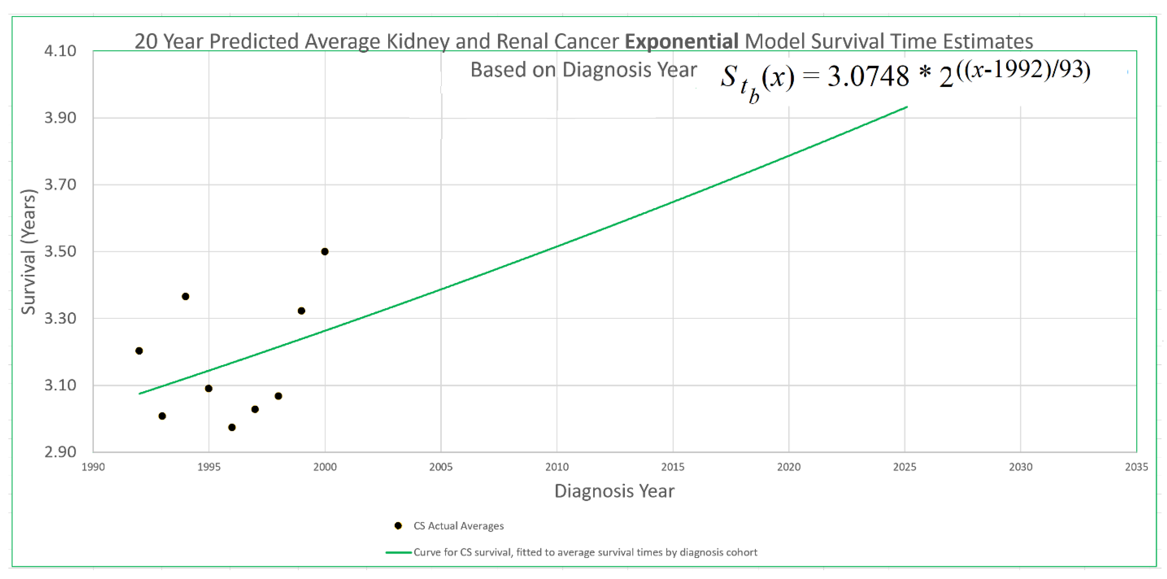
Figure 2. Twenty-year survival cohorts. The blue-and-purple horizontal bars represent diagnosis year cohorts, while the red-and-purple bars represent death year cohorts. Red cells in the top right area of the chart show relatively recent survival data included in the red-and-purple vertical 20-year cohort bars. They are used in the new method presented here but not in the base method – a problem because recent data is important. Blue cells in the horizontal blue-and-purple 20-year cohort bars contain historical data used in the base method, but not in the new method.

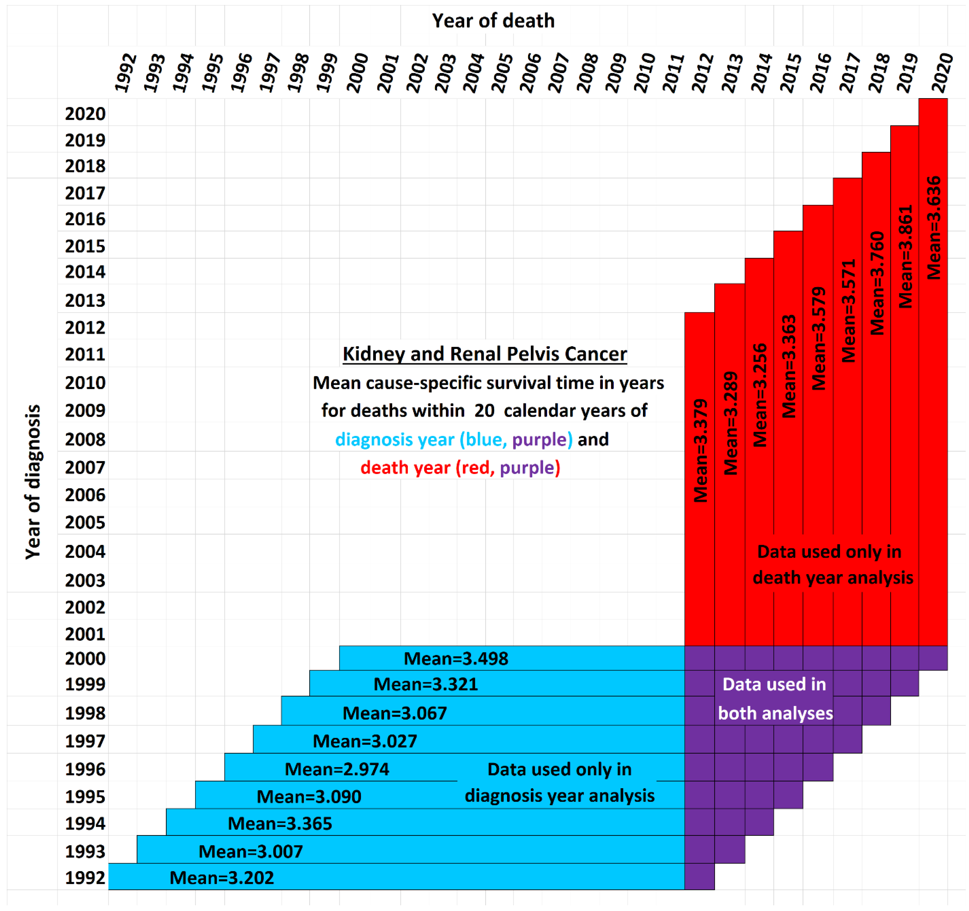
Figure 3. Updated and initial trends of improvement in 20-year cause-specific survival time for kidney and renal cancers.

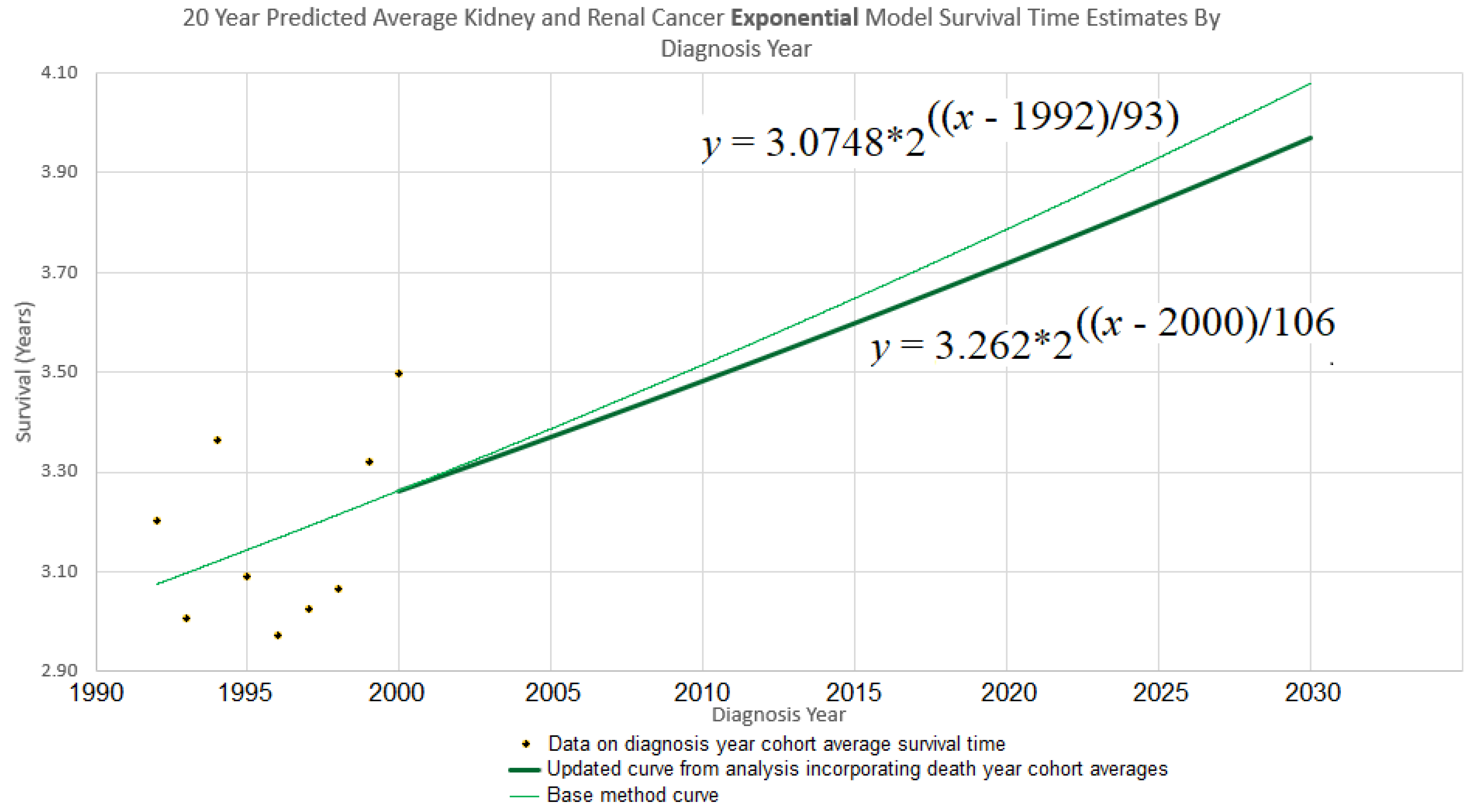
Figure 4. Kidney and renal cancer data from SEER were used to calculate average survival duration curves. These modeled the trend of improvement in average survival time over observation periods of 5 years after diagnosis year. Linear and exponential models (solid curves) were fitted to diagnosis year cohort averages (dots), and finally, updated curves were computed that additionally account for death year cohort data.

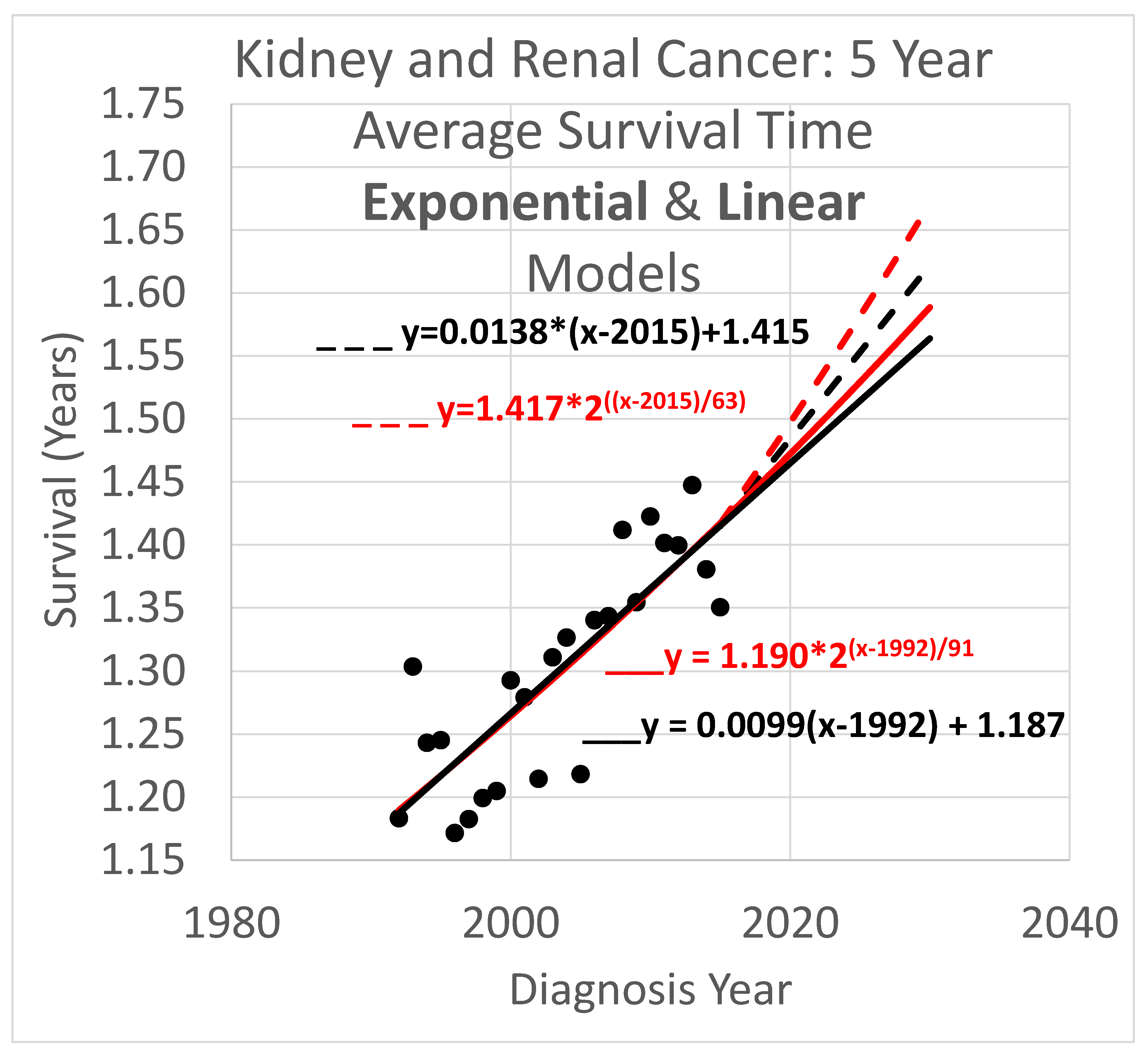
Figure 5. Trends of improvement in average survival time over observation periods of 10 years after diagnosis year.

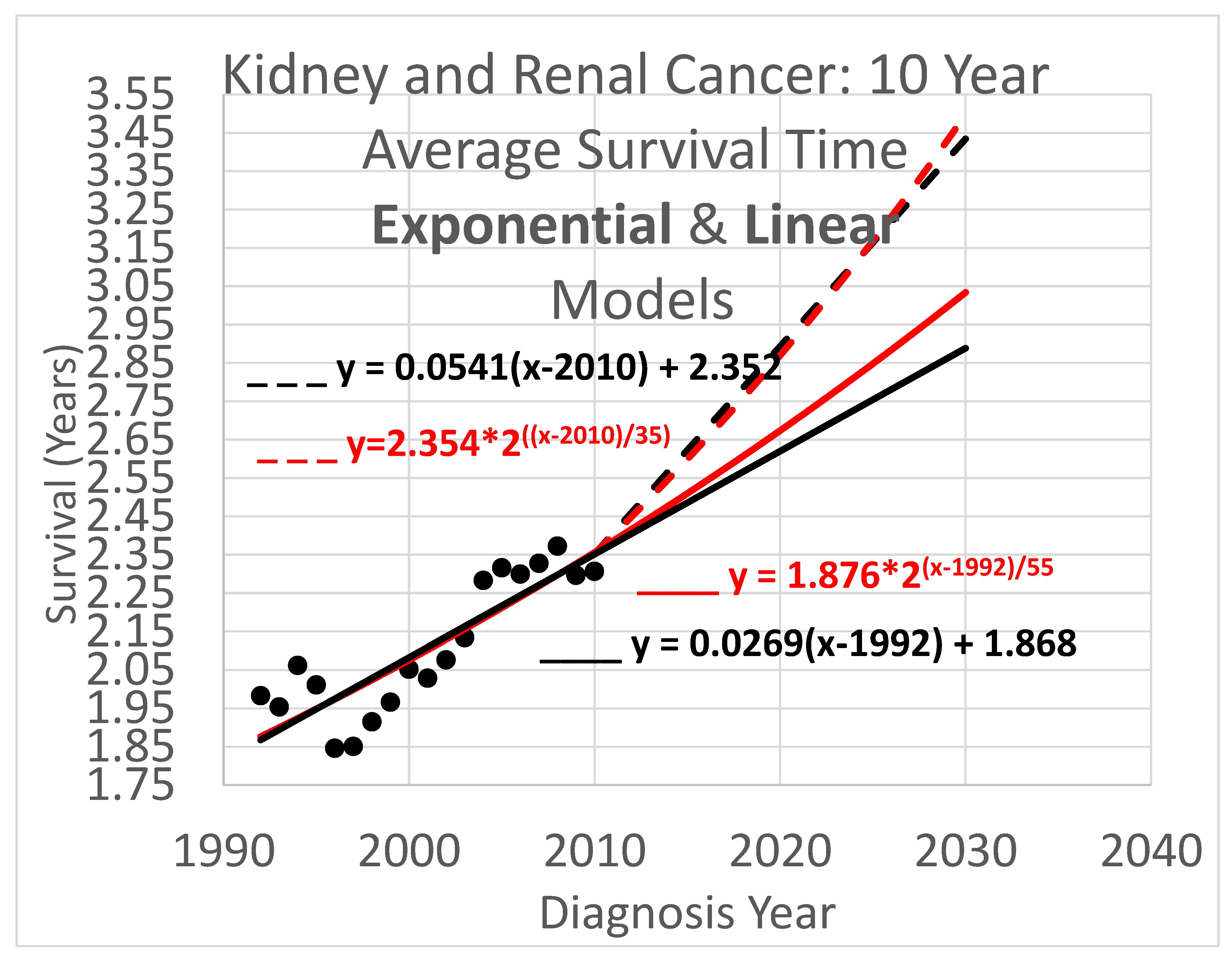
Figure 6. Trends of improvement in average survival time over observation periods of 20 years after diagnosis year.

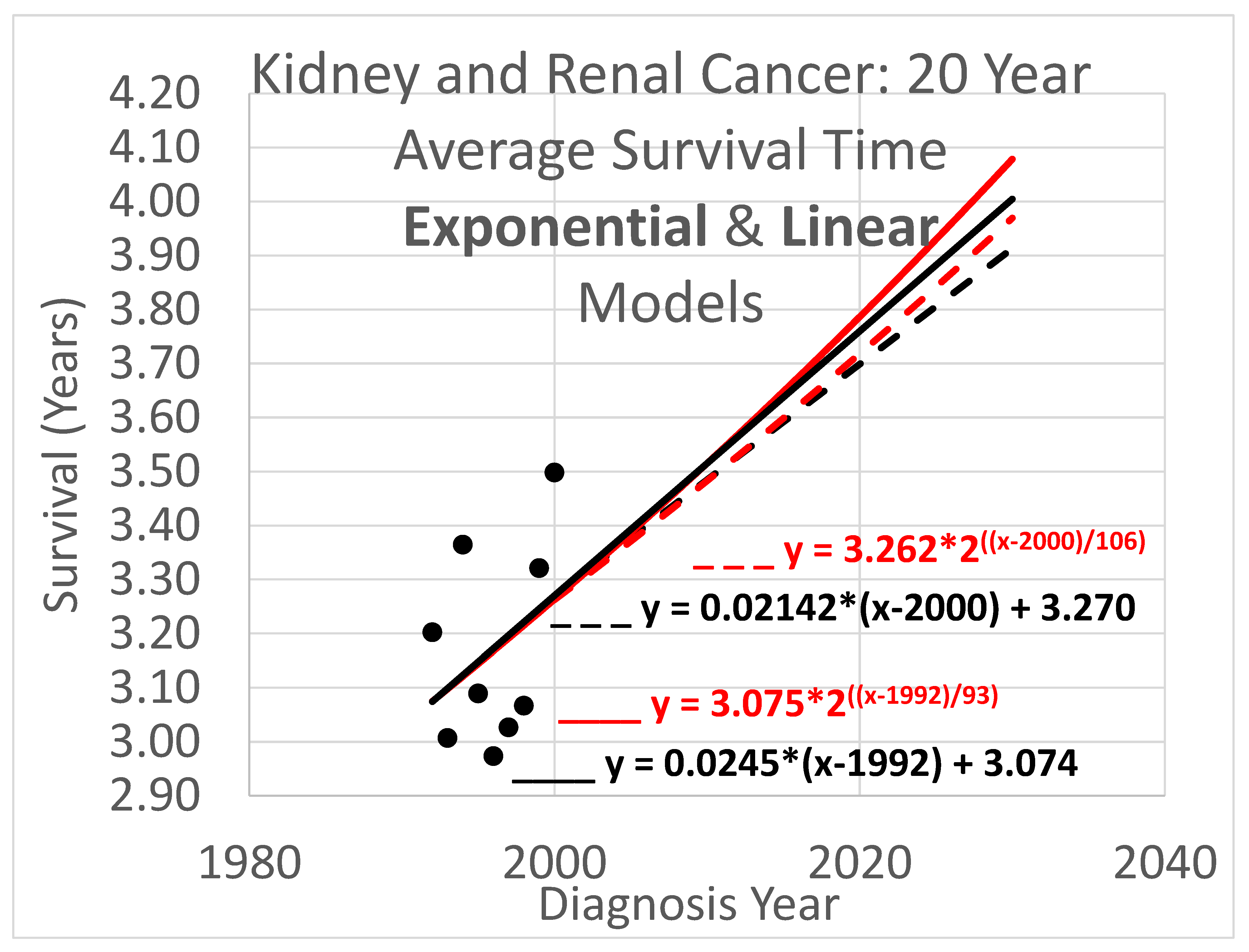
Figure 7. Number of articles published per year on Sunitinib for treatment of renal carcinoma. Sunitinib (Sutent) was approved by the FDA for treatment of renal cancer at a specific point in time, Jan. 26, 2006 (U.S. Food and Drug Administration, 2006). Yet its effects on renal cancer treatment as indicated by the number of scholarly articles published about it per year has been spread out over many years and indeed still continues (Google Scholar, 2024). (Graphing tool credit: https://mycurvefit.com).

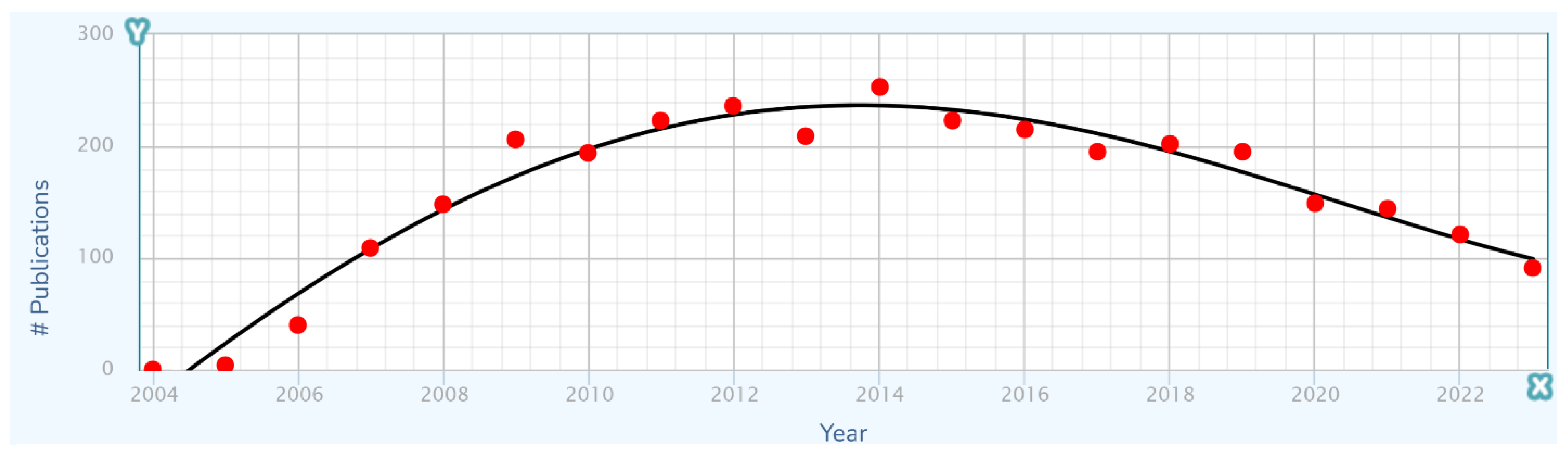
Table 1. Some specific recent advances in kidney cancer treatment.

Drug	Approved	Reference
Sunitinib	2006	(U.S. Food and Drug Administration, 2006)
Temsirolimus	2007	(U.S. Food and Drug Administration, 2007)
Pazopanib	2009	(U.S. Food and Drug Administration, 2009)
Zortress (everolimus)	2010	(Drugs.com, 2010)
Axitinib	2012	(Tyler, 2012)
Cabozantinib	2016	(U.S. Food and Drug Administration, 2016a)
Everolimus + Lenvatinib	2016	(U.S. Food and Drug Administration, 2016b)
Sunitinib adjuvant	2017	(U.S. Food and Drug Administration, 2017)
Nivolumab + ipilimumab	2018	(U.S. Food and Drug Administration, 2018)
Pembrolizumab + xitinib	2019	(Lane, 2019)
Pembrolizumab + Lenvatinib adjuvant	2021	(U.S. Food and Drug Administration, 2021a)
Nivolumab + cabozantinib	2021	(U.S. Food and Drug Administration, 2021b)
Belzutifan	2023	(Drugs.com, 2023)

Disclaimer/Publisher’s Note: The statements, opinions and data contained in all publications are solely those of the individual author(s) and contributor(s) and not of MDPI and/or the editor(s). MDPI and/or the editor(s) disclaim responsibility for any injury to people or property resulting from any ideas, methods, instructions or products referred to in the content.

© 2025 by the authors. Licensee MDPI, Basel, Switzerland. This article is an open access article distributed under the terms and conditions of the Creative Commons Attribution (CC BY) license (http://creativecommons.org/licenses/by/4.0/).

Copyright: This open access article is published under a Creative Commons CC BY 4.0 license, which permit the free download, distribution, and reuse, provided that the author and preprint are cited in any reuse.

Downloads

Views

Comments

Subscription

Notify me about updates to this article or when a peer-reviewed version is published.

MDPI Initiatives

Important Links

Choose an area of interest and we will send you notifications of new preprints at your preferred frequency.

Disclaimer