Submitted:
13 April 2025
Posted:
14 April 2025
You are already at the latest version
Abstract
This study compares mobile observation data from the same study area in Kunming on January 15, 2020, and January 8, 2023, to investigate the changes in micro-scale urban thermal environment characteristics under different weather conditions. Specifically, under overall declining temper-atures, commercial and industrial areas experience a more dramatic cooling effect. These regions, typically characterized by dense construction, limited green spaces, and abundant anthropogenic heat sources, show a more sensitive temperature response and larger cooling amplitude when ambient temperatures drop. In contrast, parks, wetlands, and other well-greened areas are less affected due to the moderating effects of vegetation and water bodies, resulting in relatively stable temperature differences. These variations lead to increased local temperature disparities, further exacerbating the unevenness of the urban thermal environment. Consequently, commercial and industrial zones are more vulnerable to thermal changes under extreme weather conditions, highlighting the fragility of urban resilience in the face of climate change.
Keywords:
Mobile Observation
; Urban Thermal Environment
; Urban Functional Areas
; Climate Background
1. Introduction
Urban heat islands (UHI) are one of the most prominent features of urban climate, with a more pronounced impact in densely populated cities. The urban heat island effect refers to higher air temperatures in urban areas compared to surrounding rural or natural environments[1]. Fundamentally, urban heat islands are caused by widespread changes in urban surface properties and construction materials, as continuous urbanization globally exacerbates heat island effects[2,3]. Land use and coverage changes will become one of the primary drivers of urban spatial expansion[4,5]. However, different surface properties of land cover types can lead to significant fluctuations in the thermal environment within urban areas[6]. Various land cover types, such as green spaces, built-up areas, bare land, and water bodies, absorb, store, and release heat in different ways, resulting in notable temperature differences across regions[7]. Urban green spaces have a higher evapotranspiration cooling effect, which helps lower temperatures through evaporation, while built-up areas and bare land, with their lower heat capacity and enhanced heat island effect, tend to accumulate heat, raising the surrounding temperature[8]. Water bodies, on the other hand, reduce temperatures through evaporative cooling, though this effect is influenced by the size and depth of the water body[9]. These varying surface properties not only affect the temperature levels in different regions but may also lead to frequent temperature fluctuations[10]. For instance, during urbanization, changes in land use types can cause varying degrees of urban heat island effects across different areas, leading to the emergence of extreme heat or relatively cooler areas in localized regions[11]. As climate change and urbanization accelerate, these fluctuations may intensify, further impacting the overall urban thermal environment [12,13].
The rapid urbanization process has on the surface, altered the urban landscape, creating modern, bustling cities with high-rise buildings and concentrated populations. On a deeper level, it has changed the original urban climate and ecological environment, impacting urban energy budgets and energy balance. Regarding the impact of extreme weather-induced thermal and humid environmental changes on human health, global researchers have conducted extensive studies. [14] analyzed the long-term changes in heat exposure in densely populated areas and emphasized the potential impact of changes in urban humid environments on public health. [15] found a correlation between urban greening, temperature, humidity, and cardiovascular diseases, suggesting that the urban humid environment significantly influences residents' health. [16] further revealed the association between air pollution and the incidence of allergic rhinitis, noting that air temperature and relative humidity directly affect air pollution levels. Additionally, [17,18] studies have shown that extreme heatwaves lead to severe morbidity and mortality rates, exploring the synergistic effect of high temperatures and humidity on non-accidental deaths, with the risk of death increasing with the duration of high temperature and humidity.
However, most studies on urban thermal environments and extreme weather primarily rely on satellite imagery and remote sensing models to assess the impact of urbanization on urban heat island intensity and land surface temperature (LST)[19,20]. This method has limitations in reflecting thermal environment differences and fluctuations under different land cover types in urban areas. Remote sensing data typically only provide temperature change information at a macro scale[21], making it difficult to capture dynamic temperature fluctuations in fine-scale areas. In contrast, this study uses a mobile observation method, leveraging high-density field measurement data to more accurately capture temperature fluctuations and distributions of the urban thermal environment under different land cover types. Compared to remote sensing observations, mobile observations can dynamically reflect thermal environment changes in real-time, especially capturing the subtle impacts of land cover on thermal environments at fine scales. For example, different land cover types (such as green spaces[22], built-up areas[19], bare land[23], and water bodies[24]) absorb, store, and release heat in different ways, leading to significant temperature differences and fluctuations in localized areas. Mobile observations can reflect these temperature fluctuations more accurately and provide more representative field data[25,26,27]. Unlike the static nature of remotely sensed data, mobile observations can provide more realistic data on dynamic temperature changes, thus revealing in greater depth the changes in the thermal environment of different urban areas.
By combining mobile observation data from January 15, 2020, and January 8, 2023, under different weather backgrounds, this study highlights the importance of examining sensitivity to weather changes. The comparison of data from these two days not only analyzes changes in the urban thermal environment under different meteorological conditions but also investigates the dynamic impact of different weather backgrounds on the urban thermal environment. By comparing the thermal environment responses of the same areas under temperature changes and extreme weather conditions, the study reveals the differences in thermal environment performance in different urban functional areas when faced with varying temperature conditions. The use of mobile observation methods and comparative analysis under different weather backgrounds not only provides more detailed observational data on the dynamic changes in urban thermal environments but also offers a new perspective on the thermal environment differences in various functional areas under different climatic conditions. This provides more actionable references for future urban planning, thermal environment management, and responses to extreme climate changes.
2. Materials and Methods
2.1. Study Area
Kunming, the capital of Yunnan Province, is located in the central part of the Yungui Plateau, between 102°10' and 103°40' E and 24°23' and 26°22' N. Chenggong District, as the administrative center of Kunming and the new campus site for several universities in Yunnan, has experienced significant urbanization in recent years. Dramatic changes in land use and evident population agglomeration have made it a core area characterized by dense foot traffic and frequent activities. The rapid urbanization in Chenggong District has resulted in a more complex distribution of thermal environment characteristics, making it a representative area for studying the micro-scale urban thermal environment.
2.2. Data Collection
2.2.1. Weather Station Data
This study is based on mobile observation data and recordings from the self-installed Davis weather station, aiming to analyze the thermal environment changes in Kunming's micro-scale areas. For the mobile observation dates of January 15, 2020, and January 8, 2023, the maximum, minimum, and average temperatures were recorded to compare the weather background and thermal environment differences between the two observations. These data were obtained from the China Meteorological Data Service Center (data.cma.cn) and China Weather (weather.com.cn), providing accurate meteorological data support for the study. By comparing the temperature changes under different weather backgrounds, this study further reveals the thermal environment response differences in various urban functional areas of Kunming under different climatic conditions, offering valuable references for future urban thermal environment management and planning.
2.2.2. Mobile Observation Data
The mobile observations for this study were collected from selected areas in Chenggong District, Kunming, and temperature data were collected on January 15, 2020 and January 8, 2023, along the observation routes. These data were obtained using temperature and humidity data loggers that recorded continuously at a high density of once per second. This ensures a true representation of how temperature varies with the environment. The region includes a variety of land use types.
In selecting the mobile observation route, the primary consideration was to ensure the inclusion of a variety of typical urban functional areas. These include highly commercialized zones (such as the Rainbow Yunnan First City), residential areas (like Yuhua Yuxiu and Yimingyuan), large water bodies (such as Dianchi Lake and Pan Chun Lake), agricultural land and villages (such as Wujia Ying Village and Sanchakou Village), as well as university campuses. These areas represent different levels of human activity, land use types, and ecological characteristics, facilitating a comprehensive study of the relationship between urban heat island effects and factors like land use, greenery, and traffic flow, providing multidimensional data on thermal environment changes. The mobile observation started and ended at a highway intersection approximately 600 meters northwest of Kunming South Railway Station (referred to as the Start Point and End Point, abbreviated as S&E). The total length of the route is approximately 30 kilometers. It extends westward to Huanhu East Road near Dianchi Lake, eastward to the West Square of Kunming South Railway Station, with the northern boundary being Pan Chun Lake, also known as "Qibu Chang Datangzi." The southernmost part of the route is along the ancient Dian Road-Yupu Road. As shown in Figure 4, the mobile testing passes through five residential districts: Dianchi Xingchen (RD1), Shuxiang Dadi (RD2), Yuhua Yuxiu (RD3), Yimingyuan (RD4), and Shidai Junyuan (RD5). It also passes through the middle of RD3, while RD1 is highly commercialized with numerous restaurants and shops. There are five water bodies: Dianchi Lake (WA), Bailongtan (L1), Pan Chun Lake (L2), Yueya Pond (L3), and Guanshan Reservoir (R). Among them, Dianchi Lake is a large water body with a total area of 330 km2, while the others are medium to small-sized water bodies. There are three villages: Wujia Ying Township (V1), Sanchakou Village (V2), and Kele Village (V3). Additionally, two agricultural fields (FL1, FL2), construction land (CA1), and Yunnan Radio and Television Station (TS) are present in the area. Table 1 represent the equipment information table.
2.3. Data Processing
This study mainly conducted on-site tests using a mobile observation method. When processing the data, the methods of simultaneous correction and spatial interpolation were used to reduce errors by considering potential issues such as time errors in the test results or uneven distribution of measurement points.
2.3.1. Data Processing of Raw Data
1.Temperature Data
The HOBO-ware U23-001 temperature data logger used for the testing was configured with the desired start time and recording interval using the computer software. Once the designated time was reached, the data logger automatically initiated the installation process and began recording the relative temperature data according to the present requirements.
2.GPS Data
To ensure the continuity of recorded GPS trajectories, any surplus data points can be removed during the subsequent data compilation. The GPS data can then be imported into Google Earth software to visualize the route trajectory.
2.3.2. Data Normalization
To begin the process of data normalization, the GPS trajectory data is opened, and the coordinates marking the starting and ending points are identified. The raw data from both instruments are then subjected to normalization procedures. These steps involve aligning the timestamps, performing spatial interpolation, implementing simultaneous revision, and simplifying the route trajectory data.
1.Aligning Timestamps
In this study, the temperature and humidity data logger used for testing was configured to record at a frequency of one measurement per second, which aligns with the frequency of GPS recorders capturing trajectory points. This facilitates the correspondence between the data in terms of time, temperature, relative humidity, and latitude-longitude coordinates.
2.Spatial Interpolation
During the process of mobile observation, there are often areas with significant obstructions that interfere with GPS signals, resulting in data points being lost. Therefore, it becomes necessary to utilize spatial interpolation methods to supplement the missing data points.
3.Simultaneous Revision
During the testing period, the equation for the temperature curve trend was derived through regression analysis using hourly meteorological data recorded by the self-established Davis weather station. By applying this equation, the data is revised to a common reference time. Specifically, linear regression is selected to revise the data to the midpoint of the testing period.
2.3.3. Creating Contour Maps
The temperature distribution is derived using a combination of gridding and spatial interpolation methods. First, observational data was collected, with longitude as the X-axis, latitude as the Y-axis, and temperature as the Z-axis. This three-dimensional data was imported into Surfer 15 software for gridding processing. The gridding process helps convert scattered data points into a regularly spaced grid, providing a visualization for temperature distribution over a large area. After gridding the data, a 3D wireframe graph was created to represent the spatial variation of temperature within the study area. This wireframe model intuitively shows the fluctuations of temperature at different geographical locations, helping to clearly understand the overall temperature pattern of the region. After generating the wireframe graph, the view angle was adjusted to optimize the graphic and ensure the best visualization, and the graph was calibrated to eliminate distortions caused by projection. To enhance visualization and facilitate data analysis, a scatter plot was added on top of the wireframe graph. The scatter plot provided a more detailed route view, making it easier to observe trends and outliers in temperature changes. This approach allows for a clearer representation of the relationship between temperature and geographical location, providing support for further analysis. Using this method, the study generates an intuitive and clear temperature distribution map, helping to analyze temperature fluctuations at different time points and providing an effective visual tool for understanding the spatial variation of temperature in the region.
2.4. Calculating the Fluctuation of Urban Thermal Environment
The fluctuation of the urban thermal environment can be measured by calculating the temperature amplitude and standard deviation.
The temperature amplitude refers to the difference between the maximum and minimum temperatures over a specific time period. It can be calculated using Equation 1.
ΔT=Tmax–Tmin
Where: Tmax is the highest temperature during the period. Tmin is the lowest temperature during the period.
The standard deviation is a statistical measure that quantifies the dispersion of temperature data, indicating the stability of temperature fluctuations. It can be calculated using Equation 2.
Where: Ti is the temperature at each observation point. is the mean temperature across all observation points. n is the number of observation points.
By calculating the temperature fluctuation amplitude and standard deviation, the temperature variability in the study area can be comprehensively assessed. The temperature fluctuation amplitude helps to directly understand the extreme temperature changes within the region, such as heat island effects or special weather phenomena, thus identifying potential anomalies. On the other hand, the standard deviation provides a more refined description of the regularity and extent of temperature fluctuations, making it suitable for in-depth analysis of the trends and stability of temperature variations. The combination of both measures allows for a more comprehensive reflection of the changes in the thermal environment of the study area.
3. Results
3.1. Distribution of the Thermal Environment
By plotting the mobile observation data, a 3D temperature distribution map of the study area is created, and this is combined with the measured temperature data to obtain the thermal environment distribution within the mobile observation area.
As shown in Figure 3, the temperature range on January 15, 2020, was from 9.0°C to 19.4°C, with a temperature difference of 10.4°C. In contrast, on January 8, 2023, the temperature range expanded to 4.0°C to 20.5°C, with a temperature difference of 16.5°C, indicating a significantly larger temperature variation in 2023 compared to 2020. However, according to the background temperature data on the test days shown in Table 2. The day of the first test, the maximum temperature difference was 10°C, while on the second test day, it was 13°C. Under the influence of background weather conditions, the study area experienced an increase in temperature differences. The temperature variation in the tested area changed from 10°C to 10.4°C, the temperature difference in the tested area expanded from 13°C to 16.5°C. From the overall temperature changes within the study area, the data collected on January 8, 2023, show more dramatic fluctuations, indicating a less stable thermal environment.
3.2. Fluctuations in the Thermal Environment
The thermal environment distribution map based on temperature data from flow observations can observe the temperature distribution in the region, but the specific fluctuation of the thermal environment requires specific statistics on the data, and in this study, the temperature difference is used for the observed data to represent the magnitude of fluctuation of the thermal environment, and the standard deviation of the temperature data is used to measure the degree of dispersion in the distribution of the temperature data.
From Table 3, it can be observed that there are significant differences in temperature variation and standard deviation between January 15, 2020, and January 8, 2023, reflecting the fluctuations in the thermal environment of the study area over the two years. During the testing period on January 15, 2020, the temperature differences were relatively small, with a maximum of 1.3°C and a minimum of 1.0°C. These small temperature differences indicate that, during 2020, temperature changes in the study area were relatively stable, and the thermal environment remained stable. In terms of standard deviation, the values on January 15, 2020, were relatively low, with 0.24°C, 0.29°C, and 0.34°C, which further indicates that the thermal environment in 2020 had small fluctuations, with temperature changes being more regular and stable. In contrast, on January 8, 2023, the standard deviation values increased significantly, especially during the afternoon and evening periods, where the standard deviation reached 2.43°C and 1.28°C, respectively. These larger standard deviation values indicate that, during 2023, the temperature fluctuations in the study area were more intense, with a larger range of variation, and the thermal environment became more unstable.
In order to get a better view of the distribution of the mobile observations, box plots of the two data were plotted, and when combined with Figure 4 and the tabular data, the temperatures in all periods of the 2023 test are lower than the 2020 results, which is consistent with the individual test days. However, the box plots provide a more visual representation of the distribution of the test data, with the shorter purple boxes indicating concentrated temperature data, less fluctuating thermal environments, and stable thermal environments, but higher overall temperatures. While the longer yellow boxes indicate more dispersed temperatures, larger regional temperature differences, and an unstable but overall cooler thermal environment. the median of the 2023 data is located at the bottom of the box while the median of the 2020 data is located at the top of the box, suggesting that the 2023 temperature data is on the cool side, with more cool readings compared to 2020, which coincides with the decrease in hotter areas seen in the 3D distribution plot.
To better compare the differences in air temperatures between different land use types, the study collected data on the average air temperatures in different urban functional areas for each time period during the two test periods (Figure 5).
Based on the test data from January 15, 2020, and January 8, 2023, a comprehensive analysis of temperature variations across different urban functional areas during various time periods reveals significant differences in thermal environment responses under different weather backgrounds. On the morning of January 15, 2020 (08:30), temperatures in industrial, residential, village, urban, and green areas were relatively high, whereas on the morning of January 8, 2023 (09:30) temperatures dropped dramatically, with the industrial area showing the most pronounced decrease of 10.2°C, indicating an overall colder temperature background in 2023. During the afternoon test (15:30), temperatures in 2023 were generally higher than those in 2020; specifically, temperatures in industrial, residential, and green areas increased by 15.0°C, 7.8°C, and 9.2°C, respectively, while the village area increased by only about 8.5°C, reflecting that weather conditions lead to more pronounced heat accumulation in densely built, sparsely green areas. In the evening test (20:30), temperatures in 2023 again fell below those in 2020, with cooling of 11.2°C and 5.2°C in the industrial and residential areas, respectively, whereas the green area experienced a smaller decrease of 7.7°C. Overall, the results indicate that temperature fluctuations in the early morning and evening of 2023 increased significantly, with industrial and residential areas being particularly sensitive to temperature changes, while green areas exhibited relatively stable temperature variations, underscoring the moderating role of the natural environment in urban thermal regulation. This analysis provides quantitative support for a better understanding of the differences in thermal feedback among various urban functional areas under different weather conditions and reveals the influence of green space and building density on temperature fluctuations in urban thermal management, offering important insights for mitigating the urban heat island effect and enhancing thermal comfort.
4. Discussion
4.1. Distribution of Thermal Environment at Different Times in the Study Area
This study divided two sets of test data from the study area into three phases—temperature rise, peak, and decline—to conduct an in-depth exploration of thermal environment trends. During the temperature rise phase, the first test conducted at 08:30 showed a temperature range of 9.0°C to 9.9°C, with a regional temperature difference of only 0.9°C. In contrast, the second test conducted at 09:30 showed a temperature range of 4.0°C to 7.6°C, and the regional temperature difference increased to 3.6°C. Although the second test took place an hour later, the temperature distribution map indicated a slower warming rate in the test area, with significantly fewer high-temperature zones. Relatively high temperatures were observed only in large residential communities in the northwest and northeast corners, while surface temperatures in other areas were largely consistent with the air temperature. During the peak phase, temperatures in both test sets exceeded 19°C. The 3D temperature distribution map showed that along the routes of the first test, temperatures were relatively uniform, with a regional difference of approximately 1.5°C. Except for a slight cooling in the L1 area, the rest of the routes maintained a stable high-temperature state. In contrast, the regional temperature difference along the second test routes expanded to 6.2°C, with high-temperature areas mainly concentrated in the southeastern corners of university campuses and large residential zones. This phenomenon may be related to certain road sections within the test area where sparse greenery and open sky led to rapid heating under direct sunlight. In the nighttime cooling phase, urban temperatures began to decrease. In the first test area, most regions experienced a reasonable degree of cooling. The heat accumulated by urban building clusters was released upward during the night, causing their surface temperatures to remain higher than those of the natural wetland park below, thus presenting a clear urban heat island effect. However, the second test area exhibited an abnormal cooling pattern—contrary to expectations, the wetland park area, which should have been a low-temperature zone, recorded higher temperatures than the southeastern residential areas. Overall, the temperature distribution followed a "northwest high, southeast low" pattern. This may be attributed to the fact that some areas had not accumulated much heat in the morning, resulting in faster cooling of the surface materials. To provide a more intuitive presentation of mobile observation data distribution, box plots were also generated. Combining the 3D temperature distribution maps with tabulated data reveals that temperatures in all phases of the second test set were lower than those of the first; the shorter purple boxes in the box plots indicate that temperature data were concentrated, with smaller fluctuations and relatively stable, but overall higher temperatures, whereas the longer yellow boxes indicate a more dispersed temperature distribution, larger regional differences, and an overall cooler thermal environment. The median of the second set of data is located at the lower end of the box, while that of the first set is at the upper end, further confirming that the second test results are cooler, consistent with the reduction of high-temperature areas observed in the 3D distribution maps.
4.2. Impact of Different Urban Functional Areas on the Thermal Environment
The impacts of different urban functional areas on the thermal environment and their underlying mechanisms reveal the critical regulatory role of a city's internal structure and layout on regional thermal conditions. In urban areas, densely built zones—such as industrial, residential, and commercial districts—are characterized by extensive impervious surfaces and abundant anthropogenic heat sources, which typically lead to rapid heat absorption and local heat accumulation during the day,[28] followed by significant temperature drops at night due to fast heat dissipation, thereby resulting in an unstable thermal environment. In contrast, natural or semi-natural areas, including green spaces, wetlands, and villages, benefit from substantial vegetation cover and the regulatory effects of water bodies;[29,30] these factors enable them to buffer temperature fluctuations by absorbing, storing, and releasing heat more gradually, thus maintaining more stable regional temperatures and mitigating thermal variations under extreme climatic conditions.
Under warmer climatic conditions, the urban heat island effect resulting from heat accumulation in different functional areas is particularly pronounced, especially in densely built zones that are more prone to developing localized high-temperature areas. Green spaces and natural areas,[31,32] however, can effectively lower surrounding temperatures and improve the overall urban thermal environment. Conversely, in colder weather, the lack of sufficient heat makes the responses in heat absorption and dissipation across various regions even more sensitive. Industrial and residential areas, with less greenery and dense building structures, often experience localized overcooling and abrupt temperature drops, whereas areas with ample vegetation maintain relatively stable temperatures due to their strong thermal regulation capabilities.
These significant differences in thermal responses among various functional areas under different weather conditions not only reflect the direct influence of urban land use and structural characteristics on heat distribution but also provide important insights for urban thermal management and planning.[33] Future urban planning should fully consider the coordinated development of different functional areas, optimize building layouts, and increase green coverage and water body configurations, thereby improving the urban thermal environment, mitigating the urban heat island effect, and enhancing the city’s resilience to extreme climatic changes as well as the overall quality of life for its residents.
4.3. Research Limitations
This study employed mobile observations to obtain fine-scale thermal environment data; however, there are limitations. The observation periods and area coverage are limited, with the dataset consisting of only two tests for comparison, making it difficult to comprehensively reflect the long-term thermal environment changes in various urban functional areas. Furthermore, the data may contain errors due to meteorological conditions and equipment precision. In addition, the combined effects of complex micro-scale factors were insufficiently considered, and the mechanism explanation remains incomplete. Future research should expand the sample size and spatiotemporal scale and improve data accuracy to enable a deeper exploration of urban thermal environment change patterns.
5. Conclusions
During large-scale urban control measures, there is a significant reduction in anthropogenic heat emissions. Cities as areas with the most concentrated human activity saw some changes in their heal environment. This study draws the following conclusions:
1.As the temperature declines, the urban thermal environment undergoes significant changes, leading to a reduction in the area of urban heat islands and an increase in urban cold islands.
2.In response to the temperature drop, different urban functional areas exhibit varying thermal feedback, with industrial and residential areas being more sensitive to temperature changes, resulting in a distribution characterized by lower temperatures.
3.Temperature fluctuations in the study area have intensified; the maximum standard deviation of the 2020 test data did not exceed 0.35°C with a temperature difference of less than 1.5°C, whereas the standard deviation of the 2023 data increased significantly across all three periods, reaching up to 2.43°C, and the temperature difference expanded to 7.5°C. This indicates that the thermal environment fluctuations in the study area are significant.
Acknowledgments
This work was supported by the Yunnan Science and Technology Major Program (202402AG050011), Science and Technology Projects of Yunnan Province's Universities Serving Key Industries (FWCY-BSPY2024061).
Conflicts of Interest
The authors declare no conflict of interest.
References
- Oke, T.R. The energetic basis of the urban heat island. Quarterly Journal of the Royal Meteorological Society 1982, 108, 455. [Google Scholar] [CrossRef]
- Broitman, D.; Koomen, E. Residential density change: Densification and urban expansion. Computers, Environment and Urban Systems 2015, 54, 32–46. [Google Scholar] [CrossRef]
- Gao, Y.; Zhang, N.; Chen, Y.; Luo, L.; Ao, X.; Li, W. Urban heat island characteristics of Yangtze river delta in a heatwave month of 2017. Meteorol Atmos Phys 2024, 136, 30. [Google Scholar] [CrossRef]
- Anjileli, H.; Huning, L.S.; Moftakhari, H.; Ashraf, S.; Asanjan, A.A.; Norouzi, H.; AghaKouchak, A. Extreme heat events heighten soil respiration. Sci Rep 2021, 11, 6632. [Google Scholar] [CrossRef] [PubMed]
- Oleson, K. Contrasts between Urban and Rural Climate in CCSM4 CMIP5 Climate Change Scenarios. Journal of Climate 2012, 25, 1390–1412. [Google Scholar] [CrossRef]
- Brusseleers, L.; Nguyen, V.G.; Vu, K.C.; Dung, H.H.; Somers, B.; Verbist, B. Assessment of the impact of local climate zones on fine dust concentrations: A case study from Hanoi, Vietnam. Building and Environment 2023, 242, 110430. [Google Scholar] [CrossRef]
- Xi, Y.; Wang, S.; Zou, Y.; Zhou, X.; Zhang, Y. Seasonal surface urban heat island analysis based on local climate zones. Ecological Indicators 2024, 159, 111669. [Google Scholar] [CrossRef]
- Ornam, K.; Wonorahardjo, S.; Triyadi, S. Several façade types for mitigating urban heat island intensity. Building and Environment 2024, 248, 111031. [Google Scholar] [CrossRef]
- Zhao, J.; Zhao, X.; Liang, S.; Zhou, T.; Du, X.; Xu, P.; Wu, D. Assessing the thermal contributions of urban land cover types. Landscape and Urban Planning 2020, 204, 103927. [Google Scholar] [CrossRef]
- Shen, P.; Wang, M.; Liu, J.; Ji, Y. Hourly air temperature projection in future urban area by coupling climate change and urban heat island effect. Energy and Buildings 2023, 279, 112676. [Google Scholar] [CrossRef]
- Lin, Z.; Xu, H.; Yao, X.; Yang, C.; Ye, D. How does urban thermal environmental factors impact diurnal cycle of land surface temperature? A multi-dimensional and multi-granularity perspective. Sustainable Cities and Society 2024, 101, 105190. [Google Scholar] [CrossRef]
- Stewart, I.D.; Oke, T. Local Climate Zones for Urban Temperature Studies. Bulletin of the American Meteorological Society 2012, 93, 1879–1900. [Google Scholar] [CrossRef]
- Tao, H.; Xing, J.; Pan, G.; Pleim, J.; Ran, L.; Wang, S.; Chang, X.; Li, G.; Chen, F.; Li, J. Impact of anthropogenic heat emissions on meteorological parameters and air quality in Beijing using a high-resolution model simulation. Front. Environ. Sci. Eng. 2022, 16, 44. [Google Scholar] [CrossRef]
- Núñez, A.; García, A.M.; Moreno, D.A.; Guantes, R. Seasonal changes dominate long-term variability of the urban air microbiome across space and time. Environment International 2021, 150, 106423. [Google Scholar] [CrossRef] [PubMed]
- Klompmaker, J.O.; Hart, J.E.; James, P.; Sabath, M.B.; Wu, X.; Zanobetti, A.; Dominici, F.; Laden, F. Air pollution and cardiovascular disease hospitalization – Are associations modified by greenness, temperature and humidity? Environment International 2021, 156, 106715. [Google Scholar] [CrossRef]
- Wu, R.; Guo, Q.; Fan, J.; Guo, C.; Wang, G.; Wu, W.; Xu, J. Association between air pollution and outpatient visits for allergic rhinitis: Effect modification by ambient temperature and relative humidity. Science of The Total Environment 2022, 821, 152960. [Google Scholar] [CrossRef]
- The joint and interaction effect of high temperature and humidity on mortality in China. Environment International 2023, 171, 107669. [CrossRef]
- Shu, C.; Gaur, A.; Wang, L.; Lacasse, M.A. Evolution of the local climate in Montreal and Ottawa before, during and after a heatwave and the effects on urban heat islands. Science of The Total Environment 2023, 890, 164497. [Google Scholar] [CrossRef]
- Zhu, Z.; Shen, Y.; Fu, W.; Zheng, D.; Huang, P.; Li, J.; Lan, Y.; Chen, Z.; Liu, Q.; Xu, X.; et al. How does 2D and 3D of urban morphology affect the seasonal land surface temperature in Island City? A block-scale perspective. Ecological Indicators 2023, 150, 110221. [Google Scholar] [CrossRef]
- Zhou, L.; Yuan, B.; Hu, F.; Wei, C.; Dang, X.; Sun, D. Understanding the effects of 2D/3D urban morphology on land surface temperature based on local climate zones. Building and Environment 2022, 208, 108578. [Google Scholar] [CrossRef]
- Das, M.; Das, A. Assessing the relationship between local climatic zones (LCZs) and land surface temperature (LST) – A case study of Sriniketan-Santiniketan Planning Area (SSPA), West Bengal, India. Urban Climate 2020, 32, 100591. [Google Scholar] [CrossRef]
- Han, Y.; Qiao, D.; Zhang, Y.; Wang, J. Urban expansion dynamic and its potential effects on dry-wet circumstances in China’s national-level agricultural districts. Science of The Total Environment 2022, 853, 158386. [Google Scholar] [CrossRef]
- Yuan, B.; Zhou, L.; Hu, F.; Zhang, Q. Diurnal dynamics of heat exposure in Xi’an: A perspective from local climate zone. Building and Environment 2022, 222, 109400. [Google Scholar] [CrossRef]
- Wang, R.; Voogt, J.; Ren, C.; Ng, E. Spatial-temporal variations of surface urban heat island: An application of local climate zone into large Chinese cities. Building and Environment 2022, 222, 109378. [Google Scholar] [CrossRef]
- Acosta, M.P.; Vahdatikhaki, F.; Santos, J.; Jarro, S.P.; Dorée, A.G. Data-driven analysis of Urban Heat Island phenomenon based on street typology. Sustainable Cities and Society 2024, 101, 105170. [Google Scholar] [CrossRef]
- Kawakubo, S.; Arata, S.; Demizu, Y.; Kamata, T.; Narumi, D.; Asawa, T.; Ihara, T. Visualization of urban roadway surface temperature by applying deep learning to infrared images from mobile measurements. Sustainable Cities and Society 2023, 99, 104991. [Google Scholar] [CrossRef]
- Li, X.S.; Chen, H.; Han, M.T.; Cao, J.Y. Research on the Temperature Gradients Change from Wuhan Urban Center to Suburb in Summer. AMM 2012, 174–177, 3598–3602. [Google Scholar] [CrossRef]
- Kim, S.W.; Brown, R.D. Development of a micro-scale heat island (MHI) model to assess the thermal environment in urban street canyons. Renewable and Sustainable Energy Reviews 2023, 184, 113598. [Google Scholar] [CrossRef]
- Zhang, Y.; Du, X.; Shi, Y. Effects of street canyon design on pedestrian thermal comfort in the hot-humid area of China. Int J Biometeorol 2017, 61, 1421–1432. [Google Scholar] [CrossRef]
- Chang, Y.; Xiao, J.; Li, X.; Weng, Q. Monitoring diurnal dynamics of surface urban heat island for urban agglomerations using ECOSTRESS land surface temperature observations. Sustainable Cities and Society 2023, 98, 104833. [Google Scholar] [CrossRef]
- Hao, L.; Huang, X.; Qin, M.; Liu, Y.; Li, W.; Sun, G. Ecohydrological Processes Explain Urban Dry Island Effects in a Wet Region, Southern China. Water Resources Research 2018, 54, 6757–6771. [Google Scholar] [CrossRef]
- Gunawardena, K.R.; Wells, M.J.; Kershaw, T. Utilising green and bluespace to mitigate urban heat island intensity. Science of The Total Environment 2017, 584–585, 1040–1055. [Google Scholar] [CrossRef] [PubMed]
- Geng, S.; Yang, L.; Sun, Z.; Wang, Z.; Qian, J.; Jiang, C.; Wen, M. Spatiotemporal patterns and driving forces of remotely sensed urban agglomeration heat islands in South China. Science of The Total Environment 2021, 800, 149499. [Google Scholar] [CrossRef] [PubMed]
Figure 1.
Study Area Map.
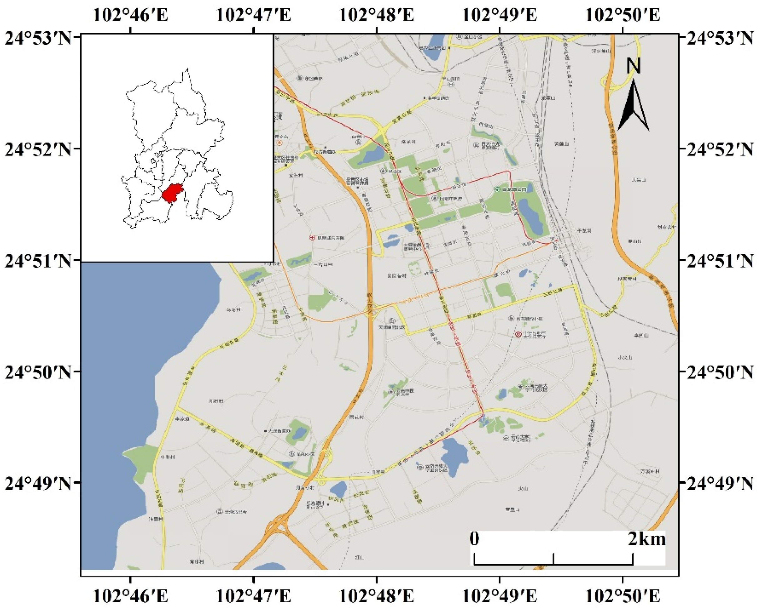
Figure 2.
Mobile measurement routes. The yellow line represents the route of the first test and the blue line represents the route of the second test. The red dots indicate the start and end points of the test.
Figure 2.
Mobile measurement routes. The yellow line represents the route of the first test and the blue line represents the route of the second test. The red dots indicate the start and end points of the test.
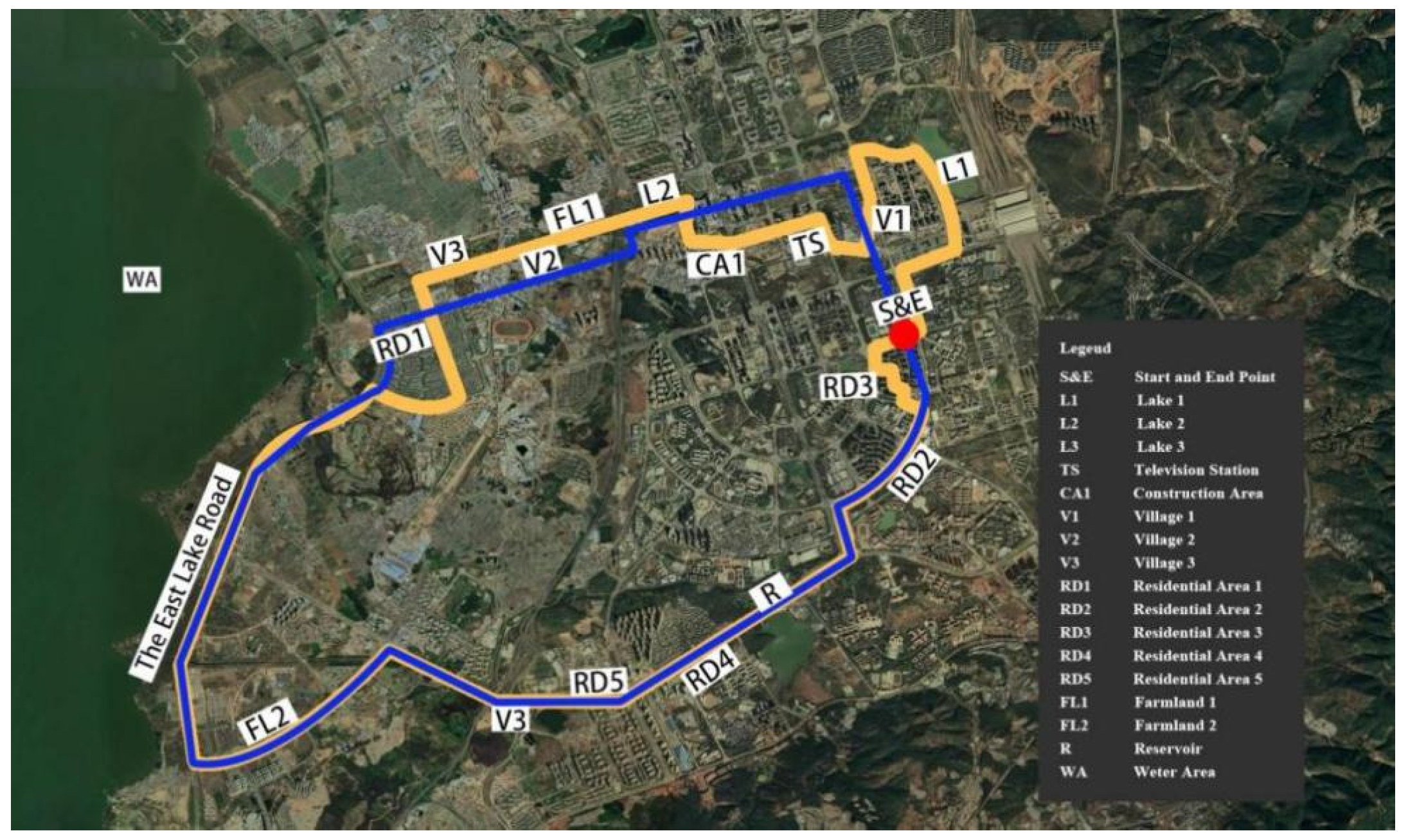
Figure 3.
Mobile Observation 3D Temperature Distribution Map: (a), (c), (e) represent the data from January 15th, 2020, while (b), (d), (f) represent the data from January 8th, 2023.
Figure 3.
Mobile Observation 3D Temperature Distribution Map: (a), (c), (e) represent the data from January 15th, 2020, while (b), (d), (f) represent the data from January 8th, 2023.
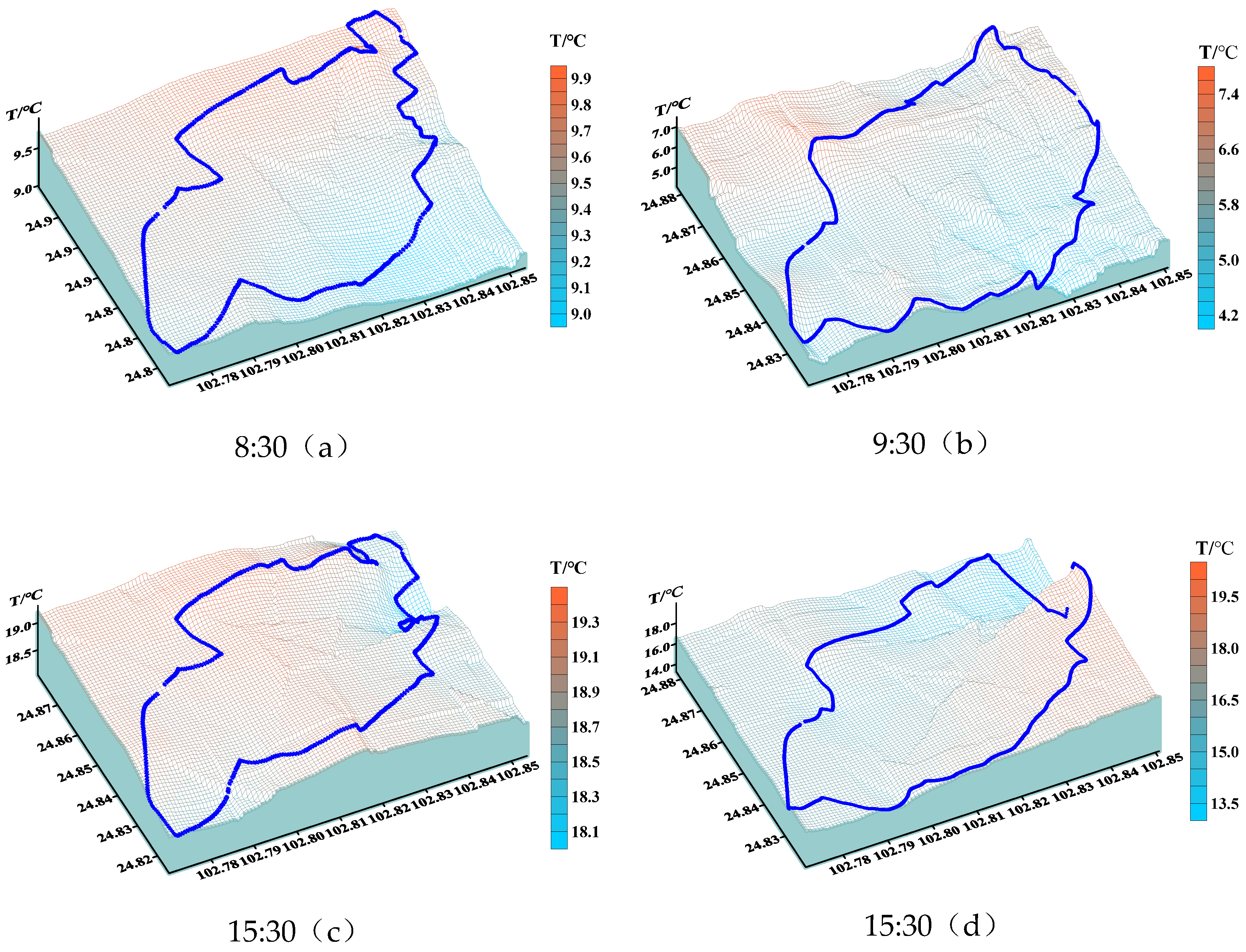
Figure 4.
Box plot of regional temperatures: purple for 2020 test data, yellow for 2023. Blue area compares temperatures during warming periods, red and gray for peak and falling periods respectively.
Figure 4.
Box plot of regional temperatures: purple for 2020 test data, yellow for 2023. Blue area compares temperatures during warming periods, red and gray for peak and falling periods respectively.
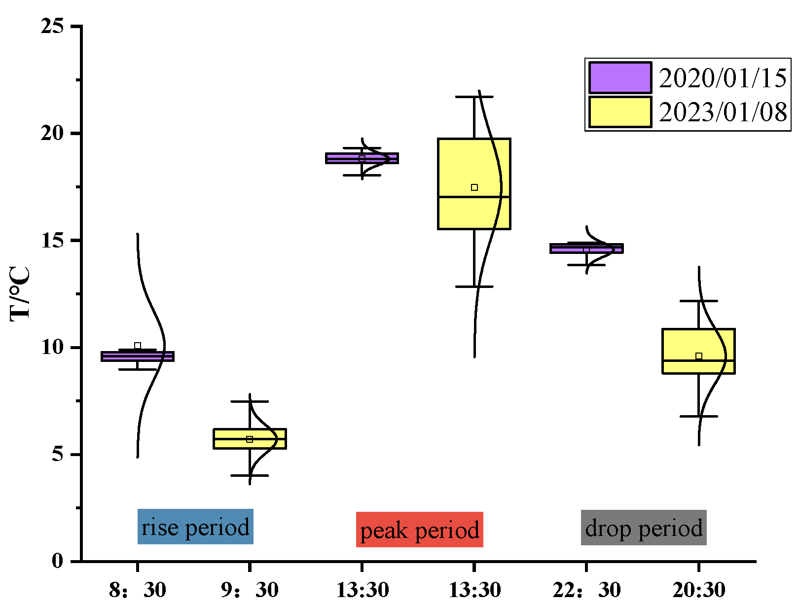
Figure 5.
Temperature comparison of different urban functional areas, with green and blue backgrounds representing the test data on January 15, 2020, and January 8, 2023, respectively.
Figure 5.
Temperature comparison of different urban functional areas, with green and blue backgrounds representing the test data on January 15, 2020, and January 8, 2023, respectively.
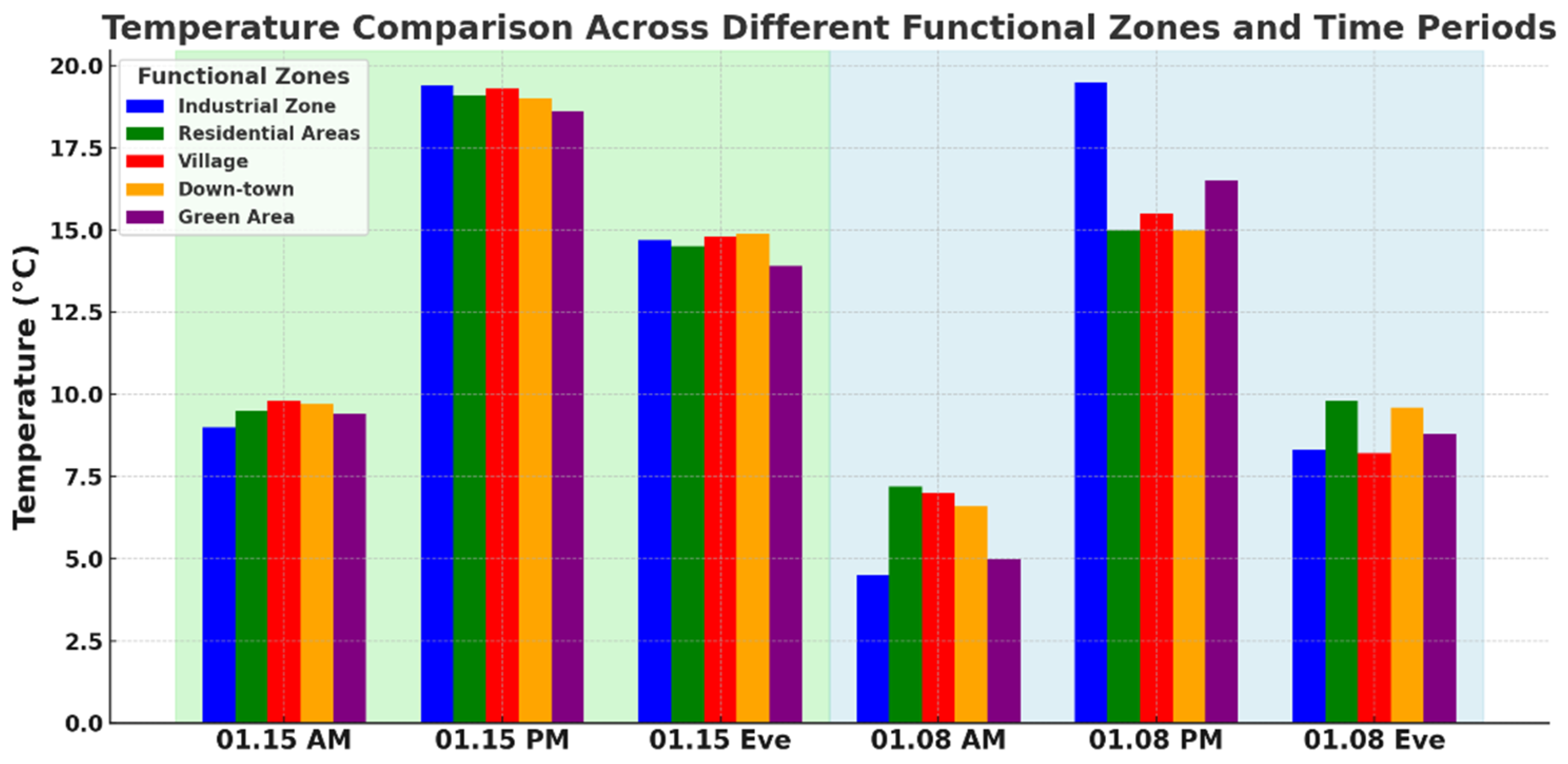

Table 1.
Table of mobile observation equipment.
| Equipment | Modes | Legends | |
|---|---|---|---|
| Professional GPS Data Logger | Columbus P-1 |
 |
The positioning accuracy of the GPS is 1.5m (horizontal) at 50% CEP (Circular Error Probable) and 4.0m at 95% CEP.” |
| Temperature/RH Data Logger | Onset MX2302A |
 |
This device has a temperature range of -40 °C to 70 °C, with measurement accuracies of ±0.25 °C below freezing and ±0.2 °C above, and a fine resolution of 0.04 °C. |
| Vehicle-mounted mobile measurement device | 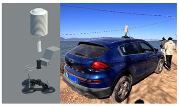 |
/ |
|
Table 2.
Temperature on Testing Dates.
| Test Date | Tmin/℃ | Tmax/℃ | ΔT/℃ | MATmax/℃ | MATmin/℃ |
|---|---|---|---|---|---|
| 2020.01.15 2023.01.08 |
9 3 |
19 16 |
10 13 |
19 16 |
10 13 |
Note: MAT(Monthly Average Temperature)
Table 3.
Table 3. Thermal environment fluctuation data within the area.
| Test Date | Testing time | Tmax/℃ | Tmin/℃ | ΔT/℃ | |
|---|---|---|---|---|---|
| 2020.01.15 | 08:30 15:30 20:30 |
9.9 19.3 14.9 |
8.9 18.0 13.7 |
1.0 1.3 1.2 |
0.24 0.29 0.34 |
| 2023.01.08 | 09:30 15:30 20:30 |
7.8 20.5 12.4 |
4.0 13.0 8.0 |
3.8 7.5 4.4 |
0.60 2.43 1.28 |
Disclaimer/Publisher’s Note: The statements, opinions and data contained in all publications are solely those of the individual author(s) and contributor(s) and not of MDPI and/or the editor(s). MDPI and/or the editor(s) disclaim responsibility for any injury to people or property resulting from any ideas, methods, instructions or products referred to in the content. |
© 2025 by the authors. Licensee MDPI, Basel, Switzerland. This article is an open access article distributed under the terms and conditions of the Creative Commons Attribution (CC BY) license (http://creativecommons.org/licenses/by/4.0/).
Copyright: This open access article is published under a Creative Commons CC BY 4.0 license, which permit the free download, distribution, and reuse, provided that the author and preprint are cited in any reuse.


