
Submitted:
22 July 2025
Posted:
23 July 2025
You are already at the latest version
Abstract
This study examines the influence of urban morphological indicators (UMIs) on both air temperature (AT) and land surface temperature (LST) in Bologna, Italy, utilizing a combination of mobile AT data and remotely sensed LST data. Nocturnal temperature 1 2 3 4 data were collected on March 19 and March 24, 2021 for AT and LST data, respectively. 5 UMIs, including building density, mean building height, floor area ratio, and vegetation 6 cover, were calculated to examine their effects on AT and LST, revealing distinct patterns in how structural and vegetative characteristics influence urban thermal conditions. After identifying significant associations between both temperatures and UMIs using Spearman’s 7 8 9 Rank correlation, a supervised linear regression model was applied to examine their 10 interaction effects. With building density emerging as the most influential factor, the model 11 yielded R-squared values of 0.77 and 0.79 for the test data of AT and LST, respectively. The 12 study provides a nuanced understanding of UHI dynamics in Bologna, offering valuable 13 insights for urban planners and policymakers seeking effective strategies to reduce urban 14 temperatures and enhance urban resilience.
Keywords:
Land Use
; Supervised Learning
; Thermal Mitigation
; Urban Forms
; Urban 16 Studies
1. Introduction
The urban heat island (UHI) effect describes the phenomenon of increased air and surface temperatures in urban areas compared to surrounding rural areas [1,2]. The UHI effect is a significant concern because it can lead to various issues, including increased energy consumption for cooling, reduced air and water quality, and negative effects on human health and biodiversity [2,3,4]. One common method of calculating UHI intensity is determining the temperature difference between urban and rural areas. However, this process is complex and requires careful consideration of factors like terrain, land cover [4]. Accordingly, selecting proper data and indicators to quantify UHI are crucial for decision-makers in developing sustainable policies.
Researchers commonly use both air temperature (AT) and land surface temperature (LST) data to investigate UHI effect [2,5]. AT is typically measured at ground-based meteorological stations, while LST is acquired through remote sensing techniques using satellite or airborne sensors [2,6,7]. While both AT and LST can quantify UHI intensity, they represent different aspects of the urban thermal environment [2,5]. Studies have shown that LST-based surface urban heat island (SUHI) intensity is generally stronger than AT-based UHI intensity, highlighting the differences in these data sources [2]. Understanding the relationship between AT and LST is essential for comprehensively assessing the UHI effect and developing effective mitigation strategies [2,5,6]. For example, research has shown that evapotranspiration from vegetation plays a significant role in reducing both SUHI and canopy urban heat island (CUHI) intensity [4]. Therefore, increasing urban green spaces, particularly through strategic urban planning and design, can help alleviate the UHI effect by promoting evaporative cooling [4,8,9]. Other mitigation methods include using cool or reflective materials for roofs and pavements to reduce heat absorption, optimizing building design and orientation to enhance natural ventilation, and reducing anthropogenic heat emissions [8,10].
The city of Bologna, Italy, has been the subject of multiple studies examining the UHI effect and potential mitigation strategies. Bologna’s diverse urban landscape, with a mix of historic and modern structures, makes it a valuable case study for understanding the complex interplay of urban morphology and UHI intensity [11,12,13,14]. Research conducted by the authors in Bologna has demonstrated the effectiveness of combining mobile and static temperature measurements for comprehensive thermal analysis [13] and has highlighted the significant impact of building density on surface temperature variations within the city [14]. These studies have provided valuable insights for urban planners and policymakers, enabling the development of targeted measures to enhance urban resilience and mitigate the negative consequences of rising temperatures and climate change.
A city’s morphological characteristics, such as building density, height, and the presence of vegetation, play a crucial role in the UHI effect [1,14]. Denser urban areas with limited vegetation tend to experience more intense UHIs due to reduced wind flow and increased heat absorption by buildings and paved surfaces [9,10,15]. On the other hand, accurate UHI characterization and quantification require a thorough understanding of these morphological influences and necessitate reliable temperature data [2]. Various Urban Morphological Indices (UMIs) are defined and studied in relation to UHI intensity studies, including building density [9,14,15,16], building height [9,15,17], sky view factor [9,15,17], green cover ratio [4,9,15], impervious plan area ratio [4,18], albedo [18], street network integration index [9], orientation variance of building [17], and mean aspect ratio [19]. Researchers use these indicators to understand how the physical layout and structure of urban areas influence UHI intensity. This knowledge helps to develop effective mitigation strategies, such as increasing green spaces, using cool materials, and optimizing building design.
To enable a more comprehensive comparative analysis of the CUHI and SUHI, this study utilizes LST data retrieved from ECOSTRESS imagery along with AT measurements acquired and corrected through a mobile survey. The primary objectives are to assess the impact of various UMIs on both AT and LST, and to investigate the correlation between AT and LST. The findings are expected to enhance understanding of UHI dynamics and assist future researchers in selecting suitable data sources and indicators for studying UHI variations.
2. Materials and Methods
2.1. Data Collection and Sources
Nocturnal AT data were collected on March 19, 2021, during a mobile transect across Bologna. Figure 1 presents a schematic diagram of the system used for AT recording. Measurements were taken along a transect path (Figure 2a), and post-processing was conducted by correcting the data with readings from fixed weather stations and thermometers positioned in various parts of the city. This adjustment was necessary to enhance the temporal accuracy and spatial relevance of the collected temperature data [13,14].
LST data for Bologna were sourced from the NASA Earth Data platform (AEEARS) [20]. The selection criteria for this data included alignment with the nocturnal timing of the AT data and minimal cloud cover (less than 10%). Based on these criteria, an ECOSTRESS image from March 24, 2021, at 16:58:54 UTC (17:58:54 local time) and with a spatial resolution of 70 meters, was chosen (Figure 2b). The ECOSTRESS mission, launched by NASA on the International Space Station in 2018, aims to measure LST and evapotranspiration using high-resolution thermal infrared data to better understand plant water use and stress across Earth’s ecosystems [21,22]. The LST data, originally in Kelvin, were converted to degrees Celsius to facilitate analysis and interpretation.
Information on buildings in Bologna was obtained from the Municipality of Bologna’s open data platform [23] (Figure 2c). This dataset provided details on the building’s height, area, and volume, which were essential for calculating UMIs. A thorough quality control process was conducted on this dataset before analysis. Temporary structures, such as kiosks and shelters, were excluded; buildings under construction were checked using historical imagery from Google Earth Pro to verify their existence in March 2021; and for buildings missing height data, Google Earth Pro 3D visualization tool was employed to estimate and fill in the missing values.
The Normalized Difference Vegetation Index (NDVI) data were derived from Sentinel-2 satellite imagery, acquired on March 24, 2021, with a spatial resolution of 10 meters (Figure 2d) [24]. From the NDVI values, the Proportion of Vegetation (PV) was calculated using Equation (1), which serves as an indicator of vegetation coverage within the study area.
where, for the NDVI imagery, min and max show the minimum and maximum values of NDVI, and PV will have a value between 0 and 1.
2.2. Block Definition and Calculation of Urban Morphology Indicators (UMIs)
To facilitate analysis along the mobile transect, spatially consistent blocks were defined based on the distance between AT measurement points. Mobile data points separated by 150 meters were selected, and each point was buffered by 150 meters. The buffer size was determined by the coarsest spatial resolution among the datasets—specifically, the 70-meter resolution of the LST data. This design ensured that each block would contain multiple measurement points for averaging, improving spatial representativeness and data reliability. In total, 352 buffers were created, which served as the analytical blocks where LST, PV, mean AT, and UMIs were calculated (Figure 3).
Based on the available data, four UMIs were selected for the analysis and calculated in a GIS environment. Equation (2) represents Mean Building Height (MBH), which indicates the average height of buildings within each defined block. Here, denotes the height of the ith building, and n is the total number of buildings that intersect with the block. Equation (3) represents Building Density (BD) defined as the total building volume () within a block per unit area of the block (A). Floor Area Ratio (FAR) is the third indicator providing an indication of building coverage intensity and is the building floor area of the ith building (Equation (4)). Finally, PV was considered as the fourth indicator (Equation (1)).
With the full dataset assembled, the next step involved removing outliers and normalizing the data. Outliers were determined by defining a lower and upper bound based on the data mean, standard deviation, and a sensitivity k value. the next step was examining the statistical relationship between AT, LST, and UMIs. Therefore, different correlation coefficients (Pearson, Spearman’s Rank, Kendall’s Tau, and partial correlations) were applied. The Pearson correlation is ideal for assessing linear associations between two continuous variables. It is most effective when the data are normally distributed and free from significant outliers [25]. Therefore, data need to be checked if they are normalized. It is done performing Shapiro-Wilk tests [26] for each dataset. However, Spearman’s Rank Correlation is a non-parametric statistical measure used to assess the strength and direction of association between two ranked variables. It is particularly useful when the data does not meet the assumptions required for Pearson’s correlation, such as linearity and normal distribution [27]. Furthermore, Kendall’s Tau correlation is particularly useful when dealing with ordinal data or non-normally distributed metric data. It measures the strength and direction of association between two variables based on their ranks, making it a robust choice for nonparametric analysis [28]. Partial correlation is a statistical technique employed to assess the relationship between two variables while controlling for the influence of one or more additional variables [29]. After normalizing the data, a stepwise linear regression considering the combination effects of UMIs was also applied. It is a supervised learning algorithm with a Sequential Feature Selection (SFS) to identify the most relevant features. SFS is a method that selects the most informative features step by step to reduce data acquisition costs and improve classification efficiency, especially when collecting data is time-consuming or expensive [30]. Procedures developed in the Python programming language were used to divide the data into two sets, 80% for training and 20% for testing. Then, stepwise linear regression was performed to obtain the relationship between UMIs and AT and LST. This analysis aimed to determine how variations in building characteristics and vegetation cover, correlate with both AT and LST, providing insight into the spatial influences of urban form on temperature distribution.
3. Results and Discussion
After removing the outliers from the data, four different correlations, Pearson, Spearman’s Rank, Kendall’s Tau, and partial, are applied to the UMIs and temperature data to get an initial insight on the influence of urban form and vegetation cover on thermal patterns. Shapiro-Wilk test [26] resulted with p-values for all the datasets of less than 0.05 which show our data were not normally distributed. Therefore, Pearson correlation could not be a good representative of the correlations. On the other hand, the partial correlation between AT and each UMIs while controlling for the influence of other UMIs were performed. It helps isolate the true effect between each two variables. The correlation between AT and MBH, BD, FAR, and PV were 47%, 18%, 10%, and 42%, respectively. Also, partial correlation between AT and LST was 61% after removing the effects of UMIs. This shows that surface temperature from Landsat is a good predictor of AT, independent of the influence of morphology. Finally, both Spearman’s Rank and Kendall’s Tau correlation performed good results. Kendall indicated the same direction as Spearman’s Rank but with lower values, which is expected due to its stricter pair comparison method. For Kendall’s Tau, LST and BD had the highest correlations with AT (70% and 59%, respectively). Similar results were found using Spearman’s Rank, with correlations of 89% between AT and LST, and 79% between AT and BD. Spearman provided the most suitable correlation values in our case (Table 1) as Kendall’s Tau is generally more appropriate for small sample sizes, while we had enough data to obtain reliable results with Spearman. Spearman’s Rank demonstrates a monotonic relationship between the data which may not necessarily be linear. This is also more robust to outliers than the other correlation methods because it ranks the data before assessing the relationship [31]. It calculates correlation based on the rank of values rather than the actual values.
Results showed a strong positive correlation between AT and BD, MBH, and FAR, with correlation coefficients of approximately 79%, 76%, and 73%, respectively. These results indicate that, as urban density and building height increase, air temperatures tend to rise, due to reduced ventilation, increased heat storage, and limited surface permeability typical of dense urban forms [9,14,15,16,17]. This positive correlation suggests that densely built environments amplify air temperatures, reinforcing the UHI effect. In contrast, PV had a negative correlation (approximately 70%). This inverse relationship implies that higher vegetation cover tends to reduce air temperatures. Vegetation cools the environment through evapotranspiration and shading, mitigating heat in urban areas [4,9,15]. This finding is consistent with the cooling effect of green spaces in urban settings, underscoring the role of vegetation in moderating urban temperatures.
When examining LST, similar to AT, a strong relationship with UMIs was derived. The correlations of LST with BD, MBH, and FAR were about 84%, 77%, and 79%, respectively, reinforcing that dense and tall urban structures retain and emit more heat. These high correlations indicate that surface temperature is particularly sensitive to urban morphology, as hard, impervious surfaces absorb solar radiation and subsequently release it as heat [32,33,34]. The link between higher LST and urban form suggests that structural characteristics are central to surface temperature patterns, further supporting the UHI phenomenon on a surface level. The relationship between PV and LST was notably negative (approximately 76%), indicating that areas with greater vegetation cover experience lower surface temperatures. This finding reaffirms the cooling function of green spaces. This outcome emphasizes that incorporating green areas into urban planning can be a strategic approach to mitigating surface temperatures and managing thermal environments in cities. Finally, a strong positive correlation was experienced between AT and LST (around 89%), suggesting that surface temperature significantly influences AT. Linear regression also yielded similar results, with an R² of 0.79 (Figure 4). The high correlation implies that areas with elevated surface temperatures are likely to experience higher air temperatures, supporting the interconnected nature of air and surface thermal characteristics. This relationship highlights the impact of surface modifications and land cover on influencing AT, as surface characteristics affect the ambient air, with implications for human comfort and health in urban settings.
Due to the particularly complex structure of Bologna, it is useful to perform a more complex model to recognize the possible interaction effects of UMIs on AT and LST. Therefore, after normalizing the data, stepwise linear regression was performed between both temperatures and UMIs (MBH, BD, FAR, and PV), as well as their interaction terms. The results from stepwise linear regression reveal both direct and interactive effects of building density, vegetation cover, and structural attributes, offering a nuanced view of urban morphology’s influence on urban heat dynamics.
Both individual and combined effects of UMIs significantly influenced AT and LST. For the influence on AT, positive effects were observed for BD and MBH, with the largest coefficient for BD (1.37), indicating that building density had a strong influence on air temperature. MBH also positively impacted AT (0.16), supporting the idea that taller buildings contribute to higher air temperatures, likely due to reduced ventilation and increased heat retention. However, FAR had an interestingly negative coefficient (-0.79) where one explanation could be that areas with higher FAR also tend to have open spaces or vertical growth that enhances ventilation, thereby lowering temperature relative to densely packed, low-rise areas. It suggests that higher FAR could lead to lower air temperatures, potentially by enabling more open ground space between structures. PV on the other hand, had a modest negative effect (-0.23), reinforcing the cooling effect of vegetation, although its impact was weaker compared to BD and MBH. Other interaction terms, such as BD_PV (0.96) and FAR_PV (-0.55), indicate that vegetation moderates the effects of building density and floor area on air temperature. The presence of these interaction terms suggests that the combination of dense urban form and vegetation influences air temperature more complexly than individual features alone. For instance, while BD tends to raise AT, the BD_PV interaction is mitigated, highlighting the vegetation moderating role (Equation (5)). The R-squared value of 0.77 suggests that the model explains approximately 77% of the variance in AT, indicating a strong model fit.
Furthermore, the model for LST highlights a slightly different pattern. BD again had the largest positive coefficient (1.81), underscoring its significant contribution to surface temperature, likely due to dense surfaces absorbing and retaining heat. Negative effect of FAR and PV, respectively -0.97 and -0.32, confirming the cooling effect of open spaces and vegetation on surface temperature. Interaction terms such as BD_PV (0.61) and FAR_PV (-0.37) indicate nuanced interactions, where vegetation moderates the warming effects of BD and FAR. Interestingly, BD_PV was positive, suggesting that dense areas with some vegetation still retain higher surface temperatures. Conversely, FAR_PV had a negative effect, implying that areas with both open floor space and vegetation experience lower surface temperatures, an optimal condition for cooling (Equation (6)). The R-squared value of 0.79 on test data indicates that this model explains about 79% of the variance in LST, slightly higher than the model for AT.
Figure 5 presents the correlation between AT and LST and their predicted values derived from the stepwise regression model, focusing solely on the test dataset. The strong alignment between observed and predicted values indicates the effectiveness of the model selection and supports the robustness of the regression approach.
Spearman correlation is a good starting point for exploratory analysis which provides us with a clear view of which individual factors correlate with temperature changes. While it is simpler and easier to interpret for assessing straightforward associations, the stepwise linear regression model provides additional layers of detail, particularly in capturing the combined effects of urban form indicators. Weng et al., (2004) [35] showed that Spearman was effective in identifying how individual features (e.g., NDVI, land cover types) correlate with LST. Furthermore, ZinZi and Agnoli (2012) [36] employed multivariate regression techniques to investigate how combinations of building characteristics and green infrastructure influence indoor-outdoor temperatures. While the Spearman correlation merely provides direct associations, the regression model identifies both direct and indirect influences, thereby offering a more comprehensive view. The R-squared values of the regression model suggest high explanatory power. This contrasts with Spearman correlation, which lacks predictive power, as it merely indicates the strength of association rather than the causative or combined impacts. For instance, while Spearman correlation does not account for interactions between indicators, such as BD_PV or FAR_PV, which play a significant role in moderating temperature, stepwise regression captures these combined effects, revealing that the relationship between urban form and temperature is not strictly additive. It is particularly useful for understanding complex urban environments where multiple factors interact. Yuan and Bauer (2007) [37] employed multiple linear regression to investigate how combinations of urban indicators influence temperature, emphasizing the value of integrated models over simple pairwise analyses. Furthermore, Oke (1982) [38] highlights that urban temperature is influenced by a combination of factors (surface materials, geometry, anthropogenic heat) and not by single variables in isolation. Our model aligns more closely with potential real-world dynamics, as urban heat dynamics are rarely influenced by isolated variables [39,40,41,42,43]. However, it requires careful interpretation, especially in the presence of multicollinearity. The selection of interaction terms could be sensitive to changes in data, and overfitting might be a risk if the model is applied to significantly different urban forms.
Furthermore, it is important to note that our analysis is limited to buffer zones constructed around selected mobile measurement points. While this approach improves data consistency along the transect and aligns with the spatial resolution of satellite data, it does not provide full coverage of the urban fabric. Therefore, the findings may not fully capture the thermal behavior of areas outside the buffered blocks. Future studies should consider expanding the spatial scope or incorporating city-wide zoning methods such as local climate zones (LCZ), land use categories, or morphological zoning [44] to improve representativeness and to reduce potential spatial bias. In this regard, the use of standardized and connected sensor systems could also enhance data coverage. For instance, recently introduced low-cost AT sensor devices, such as MeteoTracker [45], can be employed; these devices calculate the differences in heat transfer coefficients and radiant power under varying airflow conditions. They can facilitate a crowd-sourced mobile mapping of the phenomenon using a Citizen Science approach. This can involve many participants simultaneously, providing a more detailed picture of the phenomenon and increasing the level of awareness and knowledge among the community. By leveraging data collected from multiple identical devices, such a network can significantly expand the spatial and temporal resolution of urban temperature monitoring.
4. Conclusions
The study underscores the intricate relationship between urban morphology and the UHI effect, revealing both individual and combined impacts of building density, height, floor area ratio, and vegetation cover on AT and LST. Results indicate that dense, tall urban structures amplify the UHI effect by increasing AT and LST, while vegetation provides a cooling effect through evapotranspiration and shading. Spearman’s Rank correlation analyses highlight a strong positive association between AT, LST, and UMIs such as BD and MBH, which intensify the urban thermal environment by limiting ventilation and enhancing heat storage. Notably, the negative correlation of PV with both temperatures confirms that green spaces can significantly influence thermal mitigation strategies.
The stepwise linear regression analysis further reveals the nuanced influence of UMIs on thermal patterns. BD consistently shows the most substantial positive effect on both AT and LST, underscoring the role of compact urban areas in retaining heat. Interestingly, FAR exhibits a negative relationship with AT, possibly due to increased open space or vertical design in high-FAR areas that enhances ventilation. PV, although modest in effect, remains a critical factor for cooling, as shown by its interaction terms, which indicate its ability to moderate the warming impacts of BD and MBH.
The findings from this study highlight the importance of strategic urban planning in mitigating the UHI effect. By emphasizing the cooling benefits of vegetation and the role of urban design in temperature modulation, the study provides actionable insights for urban planners and policymakers. Incorporating green spaces and considering building layout can significantly reduce urban temperatures, promoting sustainable, comfortable urban environments. This research advances understanding of UHI dynamics and can guide future studies on selecting optimal data and indicators for UHI analysis, especially in cities with complex structures like Bologna. Additionally, while our study focused on buffer-based block analysis, adopting a LCZ approach could provide a more systematic and standardized classification of urban forms and thermal behaviors. Incorporating LCZs in future work would allow for a more comprehensive comparison between different urban typologies and strengthen the generalizability of the findings.
Funding
This study was partially carried out within the Space It Up project funded by the Italian Space Agency, ASI, and the Ministry of University and Research, MUR, under contract n. 2024-5-E.0 - CUP n. I53D24000060005.
Abbreviations
The following abbreviations are used in this manuscript:
| AT | Air Temperature |
| BD | Building Density |
| CUHI | Canopy Urban Heat Island |
| FAR | Floor Area Ratio |
| LCZ | Local Climate Zones |
| LST | Land Surface Temperature |
| MBH | Mean Building Height |
| NDVI | Normalized Difference Vegetation |
| PV | Proportion of Vegetation |
| SFS | Sequential Feature Selection |
| UHI | Urban Heat Island |
| UMIs | Urban Morphology Indicators |
References
- Di Sabatino, D.; Barbano, F.; Brattich, E.; Pulvirenti, B. The multiple-scale nature of urban heat island and its footprint on air quality in real urban environment. Atmosphere 2020, 11, 1186. [Google Scholar] [CrossRef]
- Yang, C.; Yan, F.; Zhang, S. Comparison of land surface and air temperatures for quantifying summer and winter urban heat island in a snow climate city. Journal of environmental management 2020, 265, 110563. [Google Scholar] [CrossRef]
- Rodríguez, L.R.; Ramos, J.S.; Domínguez, S.Á. Simplifying the process to perform air temperature and UHI measurements at large scales: Design of a new APP and low-cost Arduino device. Sustainable Cities and Society 2023, 95, 104614. [Google Scholar] [CrossRef]
- Venter, Z.S.; Chakraborty, T.; Lee, X. Crowdsourced air temperatures contrast satellite measures of the urban heat island and its mechanisms. Science Advances 2021, 7, eabb9569. [Google Scholar] [CrossRef]
- Gawuc, L.; Jefimow, M.; Szymankiewicz, K.; Kuchcik, M.; Sattari, A.; Struzewska, J. Statistical modeling of urban heat island intensity in warsaw, poland using simultaneous air and surface temperature observations. IEEE Journal of Selected Topics in Applied Earth Observations and Remote Sensing 2020, 13, 2716–2728. [Google Scholar] [CrossRef]
- Li, L.; Zha, Y.; Wang, R. Relationship of surface urban heat island with air temperature and precipitation in global large cities. IEcological Indicators 2020, 117, 106683. [Google Scholar] [CrossRef]
- Mendez-Astudillo, J.; Lau, L.; Tang, Y.-T.; Moore, T. Determination of air urban heat island parameters with high-precision GPS data. Atmosphere 2022, 13, 417. [Google Scholar] [CrossRef]
- Almeida, C.R.; de Teodoro, A.C.; Gonçalves, A. Study of the urban heat island (UHI) using remote sensing data/techniques: A systematic review. Environments 2021, 8, 105. [Google Scholar] [CrossRef]
- Güller, C.; Toy, S. The Impacts of Urban Morphology on Urban Heat Islands in Housing Areas: The Case of Erzurum, Turkey. Sustainability 2024, 16, 791. [Google Scholar] [CrossRef]
- Equere, V.; Mirzaei, P.A. : Riffat, S. Definition of a new morphological parameter to improve prediction of urban heat island. Sustainable Cities and Society 2020, 56, 102021. [Google Scholar] [CrossRef]
- Nardino, M.; Cremonini, L.; Crisci, A.; Georgiadis, T.; Guerri, G.; Morabito, M.; Fiorillo, E. Mapping daytime thermal patterns of Bologna municipality (Italy) during a heatwave: A new methodology for cities adaptation to global climate change. Urban Climate 2022, 46, 101317. [Google Scholar] [CrossRef]
- Nardino, M.; Cremonini, L.; Georgiadis, T.; Mandanici, E.; Bitelli, G. Microclimate classification of Bologna (Italy) as a support tool for urban services and regeneration. International Journal of Environmental Research and Public Health 2021, 18, 4898. [Google Scholar] [CrossRef]
- Zeynali, R.; Bitelli, G.; Mandanici, E. Mobile data acquisition and processing in support of an urban heat island study. The International Archives of the Photogrammetry, Remote Sensing and Spatial Information Sciences 2023, 48, 563–569. [Google Scholar] [CrossRef]
- Zeynali, R.; Mandanici, E.; Sohrabi, A.H.; Trevisiol, F.; Bitelli, G. GIS-Based Urban Heat Island Mapping and Analysis: Experiences in the City of Bologna. Presented at the 2024 IEEE International Workshop on Metrology for Living Environment (MetroLivEnv), IEEE 2024, 230–234.
- Liu, B.; Guo, X.; Jiang, J. How urban morphology relates to the urban heat island effect: A multi-indicator study. Sustainability 2023, 15, 10787. [Google Scholar] [CrossRef]
- Cafaro, R.; Cardone, B.; D’Ambrosio, V.; Di Martino, F.; Miraglia, V. A New GIS-Based Framework to Detect Urban Heat Islands and Its Application on the City of Naples (Italy). Land 2024, 13(8), 1253. [Google Scholar] [CrossRef]
- Lin, A.; Wu, H.; Luo, W.; Fan, K.; Liu, H. How does urban heat island differ across urban functional zones? Insights from 2D/3D urban morphology using geospatial big data. Urban Climate 2024, 53, 101787. [Google Scholar] [CrossRef]
- Shi, Y.; Zhang, Y. Urban morphological indicators of urban heat and moisture islands under various sky conditions in a humid subtropical region. Building and Environment 2022, 214, 108906. [Google Scholar] [CrossRef]
- Yang, J.; Ren, J.; Sun, D.; Xiao, X.; Xia, J.C.; Jin, C.; Li, X. Understanding land surface temperature impact factors based on local climate zones. Sustainable Cities and Society 2021, 69, 102818. [Google Scholar] [CrossRef]
- AρρEEARS. Available online: https://appeears.earthdatacloud.nasa.gov/task/area (accessed on 13 November 2024).
- Fisher, J.B.; Lee, B. : Purdy, A.J.; Halverson, G.H.; Dohlen, M.B.; Cawse-Nicholson, K.; Wang, A.; Anderson, R.G.; Aragon, B.; Arain, M.A. ECOSTRESS: NASA’s next generation mission to measure evapotranspiration from the international space station. Water Resources Research 2020, 56, e2019WR026058. [Google Scholar] [CrossRef]
- Hulley, G.C.; Göttsche, F.M.; Rivera, G.; Hook, S.J.; Freepartner, R.J.; Martin, M.A.; Cawse-Nicholson, K.; Johnson, W.R. Validation and quality assessment of the ECOSTRESS level-2 land surface temperature and emissivity product. IEEE Transactions on Geoscience and Remote Sensing 2021, 60, 1–23. [Google Scholar] [CrossRef]
- CARTA TECNICA COMUNALE - Edifici volumetrici. Available online: https://opendata.comune.bologna.it/ (accessed on 13 November 2024).
- Copernicus Data Space Ecosystem. Available online: https://browser.dataspace.copernicus.eu/ (accessed on 13 November 2024).
- Schober, P.; Boer, C.; Schwarte, L.A. Schober, P.; Boer, C.; Schwarte, L.A. Correlation coefficients: appropriate use and interpretation. Anesthesia & analgesia 2018, 126(5), 1763–1768.
- Ogunleye, L.I.; Oyejola, B.A.; Obisesan, K.O. Comparison of some common tests for normality. International Journal of Probability and Statistics 2018, 7, 130–137. [Google Scholar]
- Hauke, J.; Kossowski, T. Comparison of values of Pearson’s and Spearman’s correlation coefficients on the same sets of data. Quaestiones geographicae 2011, 30(2), 87–93. [Google Scholar] [CrossRef]
- Brophy, A.L. An algorithm and program for calculation of Kendall’s rank correlation coefficient. Behavior Research Methods, Instruments, and Computers 1986, 18(1), 45–46.
- Brown, B.L.; Hendrix, S.B. Partial correlation coefficients. Encyclopedia of statistics in behavioral science 2005. [Google Scholar]
- Rückstieß, T.; Osendorfer, C.; Van Der Smagt, P. Sequential feature selection for classification. Presented at the Australasian joint conference on artificial intelligence, Springer 2011, 132–141.
- Sedgwick, P. Spearman’s rank correlation coefficient. Bmj 2014, 349. [Google Scholar] [CrossRef]
- Hu, Y.; Hou, M.; Jia, G.; Zhao, C.; Zhen, X.; Xu, Y. Comparison of surface and canopy urban heat islands within megacities of eastern China. SPRS Journal of Photogrammetry and Remote Sensing 2019, 156, 160–168. [Google Scholar] [CrossRef]
- Schwarz, N.; Schlink, U.; Franck, U.; Großmann, K. Relationship of land surface and air temperatures and its implications for quantifying urban heat island indicators—An application for the city of Leipzig (Germany). Ecological indicators 2012, 18, 693–704. [Google Scholar] [CrossRef]
- Sheng, L.; Tang, X.; You, H.; Gu, Q.; Hu, H. Comparison of the urban heat island intensity quantified by using air temperature and Landsat land surface temperature in Hangzhou, China. Ecological indicators 2017, 72, 738–746. [Google Scholar] [CrossRef]
- Weng, Q.; Lu, D.; Schubring, J. Estimation of land surface temperature–vegetation abundance relationship for urban heat island studies. Remote sensing of Environment 2004, 89, 467–483. [Google Scholar] [CrossRef]
- Zinzi, M.; Agnoli, S. Cool and green roofs. An energy and comfort comparison between passive cooling and mitigation urban heat island techniques for residential buildings in the Mediterranean region. Energy and buildings 2012, 55, 66–76. [Google Scholar] [CrossRef]
- Yuan, F.; Bauer, M.E. Comparison of impervious surface area and normalized difference vegetation index as indicators of surface urban heat island effects in Landsat imagery. Remote Sensing of environment 2007, 106, 375–386. [Google Scholar] [CrossRef]
- Oke, T.R. The energetic basis of the urban heat island. Quarterly journal of the royal meteorological society 1982, 108, 1–24. [Google Scholar] [CrossRef]
- Li, D.; Bou-Zeid, E.; Oppenheimer, M. The effectiveness of cool and green roofs as urban heat island mitigation strategies. Environmental Research Letters 2014, 9, 14. [Google Scholar] [CrossRef]
- Myint, S.W.; Wentz, E.A.; Brazel, A.J.; Quattrochi, D.A. The impact of distinct anthropogenic and vegetation features on urban warming. Landscape ecology 2013, 28, 959–975. [Google Scholar] [CrossRef]
- Schwarz, N.; Lautenbach, S.; Seppelt, R. CExploring indicators for quantifying surface urban heat islands of European cities with MODIS land surface temperatures. Remote Sensing of Environment 2011, 115, 3175–3186. [Google Scholar] [CrossRef]
- Stewart, I.D.; Oke, T.R. Local climate zones for urban temperature studies. Bulletin of the American Meteorological Society 2012, 93, 1879–1900. [Google Scholar] [CrossRef]
- Zhou, B.; Rybski, D.; Kropp, J.P. The role of city size and urban form in the surface urban heat island. Scientific reports 2017, 7, 4791. [Google Scholar] [CrossRef]
- Vavassori, A.; Oxoli, D.; Venuti, G.; Brovelli, M.A.; de Cumis, M.S.; Sacco, P.; Tapete, D. A combined Remote Sensing and GIS-based method for Local Climate Zone mapping using PRISMA and Sentinel-2 imagery. International Journal of Applied Earth Observation and Geoinformation 2024, 131, 1103944. [Google Scholar] [CrossRef]
- Jurato, J.; Galia, T. System and method to calculate the temperature of an external environment air corrected from the radiative error, as well as sensor device usable in such system. Iotopon Srl. U.S. Patent 2022, 11,525,745.
Figure 1.
Schematic of the mobile air temperature measurement system.
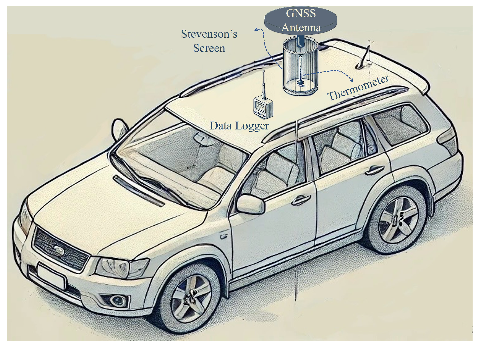
Figure 2.
Data Collection from Bologna (Italy): (a) Mobile path and air temperature, (b) Mobile path and land surface temperature, (c) Building information, and (d) Mobile path and vegetation.
Figure 2.
Data Collection from Bologna (Italy): (a) Mobile path and air temperature, (b) Mobile path and land surface temperature, (c) Building information, and (d) Mobile path and vegetation.
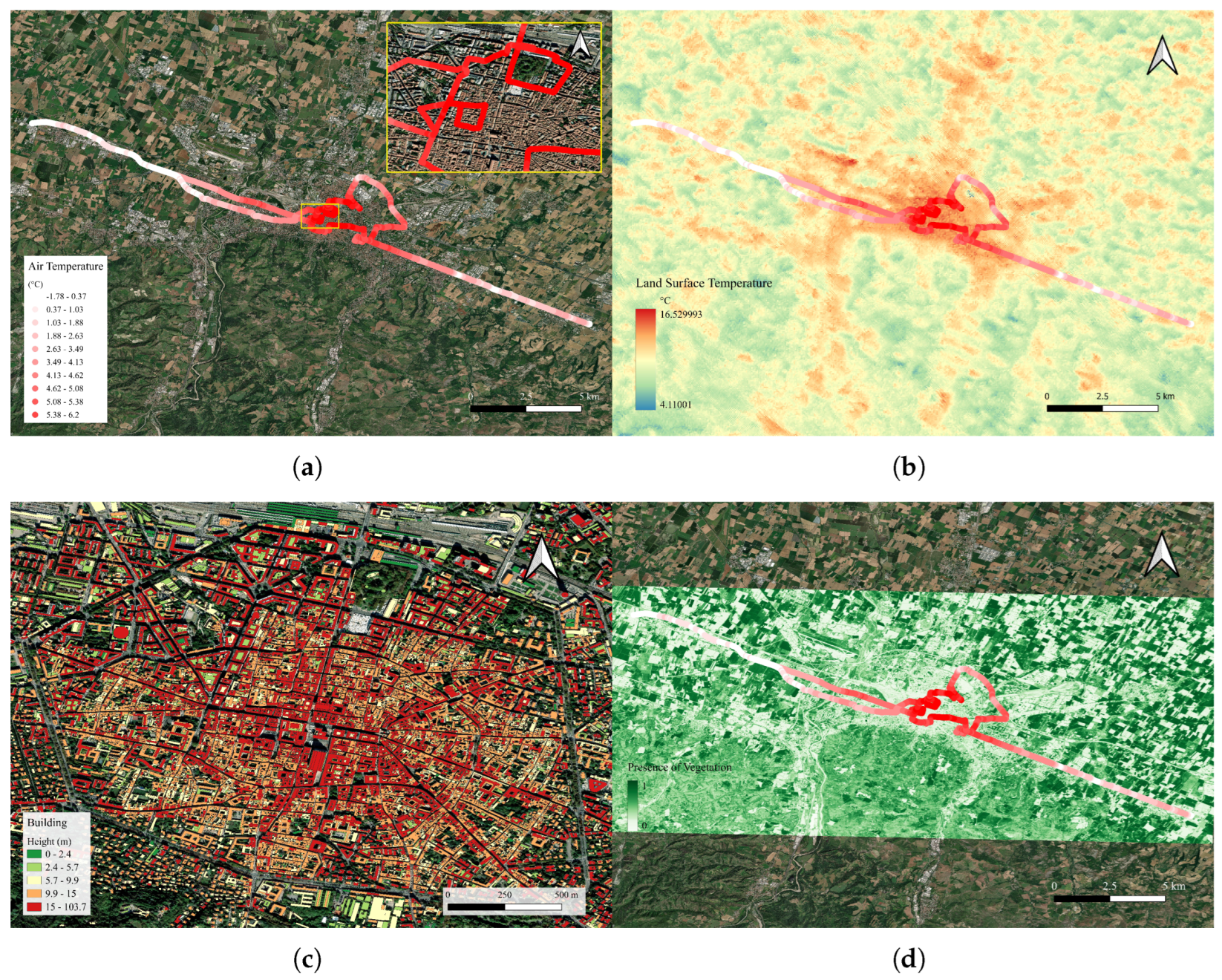
Figure 3.
Block representation (buffer areas) for various data: (a) air temperature, b land surface temperature, c building density indicator, d floor to area ratio indicator, e mean building height indicator, and f presence of vegetation indicator.
Figure 3.
Block representation (buffer areas) for various data: (a) air temperature, b land surface temperature, c building density indicator, d floor to area ratio indicator, e mean building height indicator, and f presence of vegetation indicator.
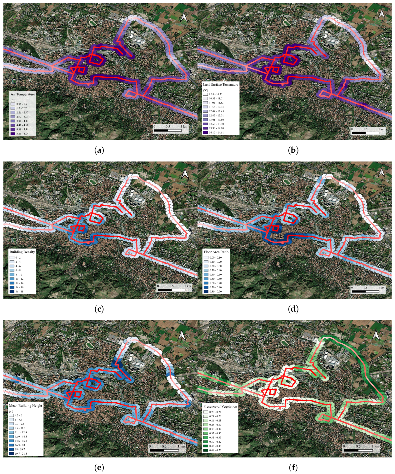
Figure 4.
Linear Regression correlation between normalized air and land surface temperatures.
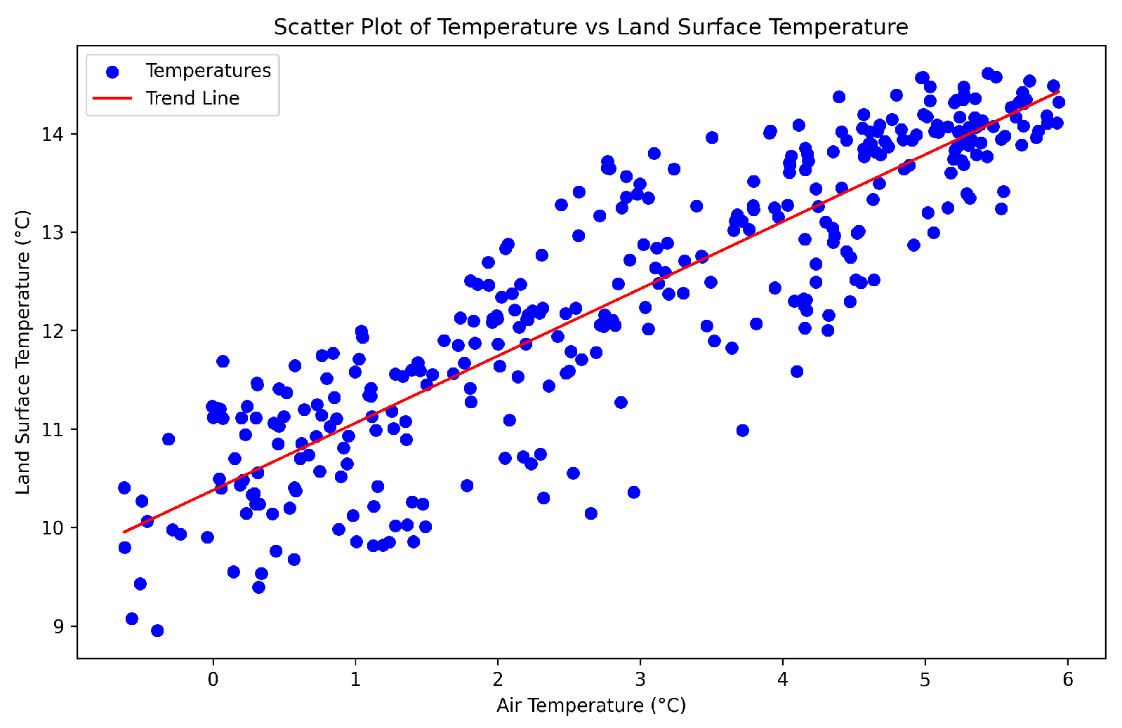
Figure 5.
Normalized temperature and predicted temperature from linear regression model for test data: (a) Air temperature, (b) Land surface temperature.
Figure 5.
Normalized temperature and predicted temperature from linear regression model for test data: (a) Air temperature, (b) Land surface temperature.
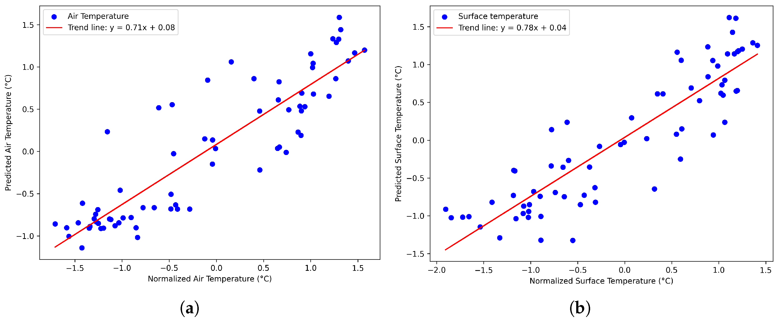

Table 1.
Spearman’s Rank correlation matrix.
| MBH | BD | FAR | PV | LST | AT | |
|---|---|---|---|---|---|---|
| MBH | 1.00 | 0.89 | 0.81 | -0.55 | 0.77 | 0.76 |
| BD | 0.89 | 1.00 | 0.97 | -0.68 | 0.84 | 0.79 |
| FAR | 0.81 | 0.97 | 1.00 | -0.68 | 0.79 | 0.73 |
| PV | -0.55 | -0.68 | -0.68 | 1.00 | -0.76 | -0.70 |
| LST | 0.77 | 0.84 | 0.79 | -0.76 | 1.00 | 0.89 |
| AT | 0.76 | 0.79 | 0.73 | -0.70 | 0.89 | 1.00 |
Disclaimer/Publisher’s Note: The statements, opinions and data contained in all publications are solely those of the individual author(s) and contributor(s) and not of MDPI and/or the editor(s). MDPI and/or the editor(s) disclaim responsibility for any injury to people or property resulting from any ideas, methods, instructions or products referred to in the content. |
© 2025 by the authors. Licensee MDPI, Basel, Switzerland. This article is an open access article distributed under the terms and conditions of the Creative Commons Attribution (CC BY) license (http://creativecommons.org/licenses/by/4.0/).
Copyright: This open access article is published under a Creative Commons CC BY 4.0 license, which permit the free download, distribution, and reuse, provided that the author and preprint are cited in any reuse.


