
Submitted:
11 April 2025
Posted:
14 April 2025
You are already at the latest version
Abstract
This work focuses on the design and development of a multilayer control architecture for a three-wheeled omnidirectional mobile robot, Robotino 4 from Festo. This modular architecture starts with an upper layer where the route to be followed by the robot is planned. The planned trajectory is then passed as a reference to an intermediate layer, where a Model-based Predictive Controller MPC computes the optimal velocity commands to follow the reference trajectory, taking into account the kinematics and the actuator constraints of the robot. Finally, these commands are processed by the lower layer, where three feedback control loops with a PID control law regulate the speed of the three wheels of the robot. To enhance autonomous navigation capabilities, the modularity of the software is analyzed by adding an obstacle avoidance module, as well as a fault detection and fault tolerance modules. In the intermediate layer, different controllers are studied, considering linear and non-linear models. A specific case of the proposed multilayer control architecture is evaluated in MATLAB using a lemniscate trajectory as reference. The simulation includes state estimation errors and motor dynamics, which are experimentally obtained, to better reflect real-world conditions. The results show the MPC capability to track the desired trajectory efficiently, with the added advantage of allowing orientation tracking. This feature offers greater flexibility compared to approaches that assume a constant orientation.
Keywords:
multilayer control architecture
; model-based predictive control
; three-wheeled omnidirectional mobile robot
1. Introduction
Research in autonomous robotics is diverse, as different robots [1], particular methodologies [2], application in simulation or navigation scenarios [3], algorithms, and software are used. The following is an excerpt of research by some authors to emphasize the difficulty of a global taxonomy.
Table 1 shows various examples of research developed on a three-wheeled omnidirectional mobile robot. These four examples use a single Robotino robot, except the work of Rokhim et. al, which uses two Robotinos. In this case, while traversing the environment, each Robotino has to leave a trace of the obstacle encountered and their traversable path, with the aim to select a more effective path and trajectory [4].
Two of the four studies use Gazebo as a simulation scenario to test the algorithms. The most complete in this sense is the work of Regier et. al, which uses a simulated scenario and an experimental indoor office to test the algorithms [5]. Testing algorithms in a real environment is more complex but allows the measurement of performance (effectiveness and efficiency). In addition, the authors conducted a statistical study, which is found to be statistically significant based on a paired t-test comparing the Dynamic Window Approach and the Proximal Policy Optimization for collision avoidance.
Some works use specific controllers in combination with the ROS architecture. The work of Mercorelli et. al applies a Model Predictive Control to optimize the trajectory of the robot [6]. In this case, a MATLAB ROS node is required to connect to the ROS architecture. The combination of MATLAB and ROS is interesting, as it allows the integration of robot motion control algorithms in MATLAB with the applicable path planning algorithms using the ROS libraries developed for this purpose, such as ROS Navigation Stack.
The work of Niemueller et. al, employs a rule-based production system using the expert system based on forward chaining inference (CLIPS, Rete algorithm) [7]. In this case, the authors prefer to use ROS, C and C++ programming, developing an external interface (where they simulate the perception inputs of the high-level decision system) and a behavior layer (where they implement a reactive behavior robot algorithm and the Adaptive Monte Carlo Localization approach).
Recent advancements in robotics suggest that frameworks must also be updated in terms of performance and algorithms [8,9]. Hence, ROS2 is a candidate for the analysis of which algorithms can be used with the three-wheeled omnidirectional mobile robot of the authors.
Following the approach developed by other researchers, this work proposes the design of a modular and scalable multilayer control architecture, providing flexibility to incorporate specific modules (e.g. obstacle avoidance). At the core of this multilayer control architecture are the kinematic model of the robot and the Model-based Predictive Control.
The objective of this work is to evaluate the performance of motion control modules in task simulation scenarios. After a brief introduction, this paper is structured as follows: the materials and methods section describes the methodology used, followed by the results section (covering both laboratory and simulation), then a discussion of the results, and finally, the conclusions with proposals for future work.
2. Materials and Methods
The main research challenges focus on validating that the three-wheeled omnidirectional mobile robot, Robotino, can be adapted as an autonomous vehicle. This includes selecting appropriate software libraries and testing their performance, refining the system architecture to operate in real time, and analyzing the possibility of designing and implementing effective planning and control algorithms.
Previous research by colleagues from the research group of the authors of this paper has demonstrated how the Berkeley Autonomous Race Car has been modified to operate autonomously. An Odroid XU4 is used to run the Robotic Operating System ROS with the control and planning algorithms [10]. For a detailed review of the literature that compares conventional automated guided vehicles with autonomous mobile robots, the work of Fragapane et al. [11] is recommended. In addition, for a comprehensive overview of mobile robot control and navigation, the work of Tzafestas provides valuable insights [12].
The methodology used in this paper is explained in the following subsections:
- Architecture. A multilayer architecture is shown following a tiered design architecture.
- Kinematic model. A mathematical model of the position and orientation of the robot and the relationship between robot velocities and wheel velocities is presented.
- Control strategy. A particular control architecture using MPC is proposed.
2.1. Architecture
The multilayer architecture proposed in Figure 1 follows a top-down approach to autonomous navigation [13,14] for the three-wheeled omnidirectional mobile robot Robotino. The architecture consists of six primary modules: Path Planning, Obstacle Avoidance, Motion Control (High-Level and Low-Level), Hardware, Fault Diagnosis, and Fault Tolerance Strategy.
The Path Planning layer is responsible for computing an optimal trajectory from the initial position of the robot to the target destination. This trajectory is then refined by the Obstacle Avoidance module, which dynamically adjusts the planned path after the detection of obstacles [15].
The Motion Control layer consists of two submodules: High-Level Control and Low-Level Control. The High-Level Control approach utilizes a MPC approach to generate optimized velocity commands in order to follow the planned trajectory while considering physical system constraints. The Low-Level Control transforms these velocity commands into individual wheel speeds, which are regulated using the PID controllers [12].
The Hardware layer consists of sensors and actuators responsible for the execution of motion and the perception of the environment. The actuators receive wheel speed commands from the PID controllers, while the sensors provide real-time feedback on the position of the robot, which is used by both the motion control and fault detection modules.
To enhance the robustness of the system, a Fault Management subsystem is integrated into the architecture, comprising two interconnected modules: Fault Diagnosis and Fault Tolerance Strategy. The Fault Diagnosis module continuously monitors the actuator performance by comparing the PID output with the sensor data to detect faults. Once a fault is detected and identified, the Fault Tolerance Strategy module determines the most suitable compensation strategy for the MPC controller to mitigate its effects and maintain stable operation.
The proposed architecture is designed to ensure modularity, scalability, and adaptability. The independent nature of each module allows for flexible modifications, such as integrating an alternative motion control strategy without altering the core framework. In addition, the architecture can be extended to other robotic platforms by adjusting system parameters and control algorithms.
Although modules are intrinsically related, when explaining the methodology, it is convenient to first introduce fundamental aspects of kinematics before linking them with MPC and PID within the overall control strategy.
2.2. Kinematics
Robotino is a holonomic mobile robot equipped with three omnidirectional Swedish 90º wheels, which are arranged equidistantly at 120-degree intervals and mounted directly on the motor shaft, sharing the same direction of rotation. Due to the nature of its wheels and their geometric configuration, the robot is capable of moving in any direction without requiring prior reorientation.
Figure 2 illustrates the Robotino configuration within a global coordinate system (), arbitrarily defined as a fixed reference frame for motion analysis. In addition, a local coordinate system () is considered, with its origin at the point P, which represents the geometric center of the robot. The orientation of the robot relative to the global system is determined by the angle .
Based on kinematic studies of three-wheeled omnidirectional mobile robots in the literature [16,17,18], the kinematic model has been adapted to the specific case of Robotino version 4. The resulting kinematic equations describe the relationship between the velocities in the global frame () and the local frame (), as well as the relationship between the motion of the robot in its reference frame and the velocities of each individual wheel ().
In Equation 1, the relation between global and local velocities is obtained using the rotation matrix in Equation 2.
To compute local velocities from global velocities, the inverse of the rotation matrix is used:
The relationship between the center of the robot velocities and the individual wheel velocities is derived from the geometric arrangement of the omnidirectional wheels. Since these wheels are placed at 120-degree intervals, the velocity of each wheel depends on both the linear and rotational motion of the robot, as expressed in Equation 5. This relationship is formulated through the Jacobian matrix J, where represent the angles between the local coordinate axis and each wheel. In the case of Robotino 4, these angles are , , and , Equation 6.
Since Robotino DC motors with permanent magnet [19] receive commands in revolutions per minute (), it is necessary to convert the linear velocities of the wheels into angular velocities, as expressed in Equation 7. In this context, the angular velocities of the motor shafts, denoted as , , and for each wheel are considered positive in the counterclockwise direction. Taking into account that the reduction ratio of the gear is (compared to Robotino 3 where the reduction ratio was [17]), and the radius of the wheels is r, the relationship between the angular velocity of the motor in and the velocity of the wheel is determined by the factor k, as given in Equation 8.
When determining the local velocities from the wheel velocities:
Once the geometric and kinematic relationships have been established, it is possible to introduce the concept of control strategy.
2.3. Control Strategy
Once the multilayer control architecture has been defined in Figure 1, a sub-level associated with the control strategy is introduced. In this context, Figure 3 shows a specific study case.
As shown in Figure 3, the subsystem follows a structured control pipeline, where a predefined trajectory, such as a lemniscate curve, is generated by the Path Planning module and provided as a reference to the Model-based Predictive Controller MPC. The MPC obtains the reference states () and optimally computes the required velocity commands in the local frame of the robot, considering the three-wheeled omnidirectional mobile robot kinematics and velocity constraints.
The computed velocity commands () are then transformed into individual wheel speeds () using the Jacobian matrix of the robot, J. These wheel speeds are regulated by a set of PID controllers, which ensure accurate tracking of the desired values [19]. The PID controllers operate at a frequency ten times higher than that of MPC.
After regulation by the PID, the wheel speeds () are transformed back into local velocity components () using the inverse of the Jacobian matrix, . These local velocities are then mapped to the global frame, taking into account the orientation of the robot, to obtain . Finally, the global velocity components are integrated over time to obtain the position of the robot ().
A State Estimation block is introduced to determine the actual position of the robot () based on sensor measurements. The estimated position is then fed back to MPC, closing the control loop.
Again, the authors proceed down a level to explain the structure of the MPC controller, providing a more detailed explanation of its implementation.
2.3.1. Model-Based Predictive Control Approach
Model-based predictive control MPC is considered High-Level Control of Robotino. The MPC controller has the ability to handle system constraints (e.g., physical feasible limits of velocity and acceleration) and optimize control inputs over a prediction horizon.
The goal of MPC in the scheme shown in Figure 3 is to ensure that the system state, defined by the global coordinates and orientation angle , follows as close as possible the reference trajectory computed by the Path Planing module. For this purpose, the MPC controller determines the optimal velocity vector in the local frame (control output ). The relation between control action and system state is obtained by discretizing Equation 1 as:
Then, the MPC controller can be defined as the following optimization problem:
where matrices Q and R determine the tracking error and control effort weights in the cost function of the optimization problem. Physical limitations are taken into account with , representing the minimum and maximum velocities, and , determine the minimum and maximum accelerations. Finally, and define the limits of the robot trajectory.
The optimization problem defined in Equation 12 is a non-linear optimization problem, but with some assumptions as fixed orientation , it can be formulated as a quadratic optimization problem. In addition, following the ideas proposed in [10], as non-linear Equation 11 can be expressed in Linear Parameter Varying form LPV, this allows to formulate the MPC problem as a quadratic optimization problem, considering a generic trajectory in the three states. The LPV control approach proves successful in research on lateral control in autonomous vehicles [20,21].
3. Results
This section presents the experimental and simulation results obtained from the proposed architecture at the beginning of this work. To validate the approach, the architecture was implemented in two distinct scenarios:
- Laboratory Scenario: Preliminary tests to verify the hardware and software of Robotino 4. In addition, experiments were performed to identify motor dynamics with the embedded PID controller and to assess state estimation errors. The results obtained from these experiments served as a basis for refining the simulation model.
- Simulation Scenario: Implements the specific study case shown in Figure 3, which includes the Path Planning layer, the High-Level Control module with MPC, and the Low-Level Control module with PID controller.
The following subsections detail the results obtained in the laboratory scenario, followed by the results from the simulation environment.
3.1. Laboratory Scenario
To ensure that the simulation scenario accurately represents the real-world behavior of the system, preliminary experiments were conducted on the Robotino 4 platform. These experiments focused on three key aspects: initial validation of system functionality, identification of motor dynamics and tuning of the PID controller, and evaluation of state estimation errors.
3.1.1. Initial Steps in Laboratory
Initial tests were performed to verify the proper functioning of the hardware and software components of the omnidirectional mobile robot. The following verifications were conducted:
- The applications of the manufacturer were tested (navigation and collision detection in Robotino View).
- The authors verified the transmission of velocity commands from an external computer running MATLAB to the robot, using its built-in REST API protocol.
- The original Robotino operating system was analyzed to ensure compatibility with ROS. In previous work [22], an autonomous navigation system was developed using ROS and Python, and its performance was evaluated in RViZ and Gazebo.
To evaluate navigation capabilities, the robot was deployed in an indoor laboratory environment (16 square meters). To assist the robot in location and orientation, fiducial markers were installed along the planned trajectory (Figure 4). The robot navigation starts at a reference frame located at the corner of the laboratory and moves toward a robotic product storage station. At the final destination, a SCARA robot performs a pick-and-place operation, placing a product on the mobile robot. Future work aims to integrate fiducial markers on a leader robot to enable autonomous following by a second robot.
Robot navigation is programmed using a sequential functional chart (see Figure 5). The program is divided into subprograms for odometry and collision detection (implemented in the Robotino View software).
The collision subprogram allows the robot to stop within a few millimeters of an obstacle. If a dynamic obstacle is detected, the robot resumes its trajectory once the object has cleared. Figure 6 shows an example of two mobile robots in close proximity. The amber light is a visual warning for nearby humans. When the robot has moved away, the first Robotino continues its autonomous navigation, with the green light indicating the absence of an obstacle.
3.1.2. Identification of Motor Dynamics and PID Tuning
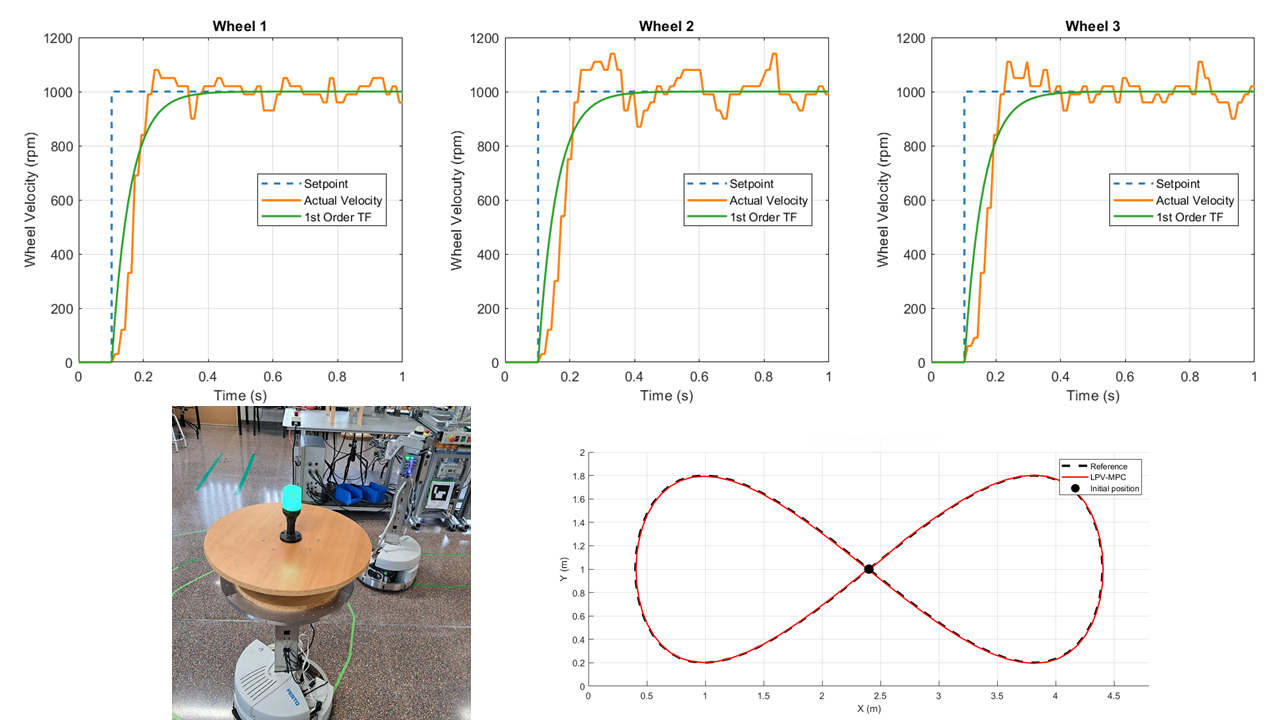
Identification of motor dynamics and PID controller was performed by applying a velocity set point of 1000 to all three motors simultaneously. The actual wheel velocities were recorded every 10 , along with their corresponding timestamps. These data were plotted (Figure 7) and analyzed.
3.1.3. Evaluation of State Estimation Errors
To evaluate the precision of state estimation, odometry-based localization was compared against ground-truth measurements obtained through manual tracking. Two open-loop experiments were conducted to quantify odometry errors under different motion conditions:
- Linear Motion Test: A constant forward velocity command of was applied for 10 seconds. Odometry readings were recorded every 10 , and the resulting trajectory is shown in the left graph of Figure 8, alongside the reference trajectory. Real-world measurements confirmed a systematic deviation due to wheel slippage, which was not considered in the odometry. Specifically, the robot exhibited an additional deviation of 5 along both the X and the Y axes.
- Rotational Motion Test: A rotational velocity command of was applied for 10 seconds, and the comparison between the reference and odometry data is shown in the right graph of Figure 8. Although odometry followed the reference rotation, real-world measurements revealed a discrepancy between the estimated and actual orientation. The observed deviation was 2 degree.
The identified motor dynamics model and the quantified state estimation errors were integrated into the simulation scenario to improve the accuracy of the virtual representation of the robot behavior.
3.2. Simulation Scenario
To evaluate the performance of the proposed LPV-MPC controller in a realistic environment, a simulation scenario was implemented in MATLAB, following the scheme presented in Figure . The system was tested using a lemniscate trajectory as reference path, which is generated by the Path Planning layer.
The LPV-MPC controller was executed at a sampling time of s, which is 10 times the constant time of the low level PID control. The following constraints were applied:
- Velocity limits:
- Acceleration limits:
- Position constraints:
-
Weighting matrices:The current setting of implies no penalization on control effort. However, in future work, this will be adjusted based on the available battery capacity of the robot to optimize energy efficiency.
- Prediction horizon:
- Initial state:
To model motor dynamics and PID, the identified first-order transfer function (obtained in Section 3.1.2) was incorporated, operating with a sampling time of s.
In addition, state estimation errors were introduced into the simulation to better approximate real-world conditions. At each iteration, an error of m was added to the x and y positions and 2 degrees to the orientation .
To evaluate the performance of the reference tracking, the Mean Squared Error (MSE) was computed for each state variable. The values obtained are shown in Table 2.
The following figures illustrate different aspects of the simulation results. Figure 9 shows the overall trajectory tracking, comparing the reference path with the motion executed. Figure 10 provides a detailed comparison of the response of the system in terms of position and orientation over time. Figure 11 evaluates actuator performance by comparing the reference and actual wheel velocities, and Figure 12 presents the tracking errors in x, y, and .
4. Discussion
Regarding the High-Level Control layer of the multilayer control architecture, there are some advantages in the use of MPC in the control of Robotino. First, obstacles considered in the path planning strategy or new ones detected on-line can be taken into account as new constraints in the optimization problem, Equation 12, in order to reduce the feasibility state space. In addition, model errors, such as state estimation errors or approximations in nonlinearities, can be taken into account in Equation 11 as
where is the actual state at time , and the term takes into account the model errors. With a matrix of appropriate dimensions, and is a vector of unknown values. If we consider unknown but bounded model errors, for example, by bounding variable unknown variable using a zonotope:
where: is a column vector of zeros with dimension (number of states) considered the center of the zonotope, ⨁ denotes the Minkowski sum, and being and m the complexity of the zonotope [24].
Then, error bounds can be computed recursively over the time prediction horizon , propagating model uncertainties. These model error bounds can be incorporated into the MPC optimization problem to ensure that the actual robot trajectories remain within physical limits and avoid obstacles despite model errors (Robust MPC [25]), as proposed in [26].
Regarding the results in Simulation Scenario, the proposed LPV-MPC approach demonstrates several advantages in High-Level Control. One of the key benefits is the ability to track a reference in orientation (), providing greater flexibility than conventional approaches that assume a constant angle [16]. This capability is important in applications requiring precise orientation adjustments, such as visual-based navigation or object manipulation.
The results obtained in Simulation Scenario, show that the robot follows the reference trajectory with minimal error. The largest deviation occurs at the beginning of the motion due to acceleration constraints, as the robot starts from a stationary position. However, this initial error rapidly decreases and the tracking error becomes nearly negligible as the trajectory progresses.
In addition, the use of the LPV formulation allows for a more efficient implementation of the initial MPC controller approach. By linearizing the system at each sampling step, the computational cost is reduced compared to nonlinear approaches while still achieving high precision in trajectory tracking. This is beneficial for real-time embedded applications where computational resources are limited.
Regarding the Obstacle Avoidance module within the sequential functional chart defined in the subsection of Initial steps in the laboratory, as a further work, the authors want to improve the program so that the robot can detect objects and execute an alternative trajectory without stopping the robot [27].
Another important aspect for future research is the Fault Management module, explained in the Architecture subsection. A specific focus will be placed on motor failures, where the MPC controller can be dynamically reconfigured to compensate for a faulty actuator. This would enable the robot to continue its navigation or, in case of critical failure, determine whether the task should be transferred to a second robot as a substitute.
In terms of cooperative navigation, the system will be extended to coordinate two mobile robots in material handling tasks. One of the robots has a tray for transporting obstacles, while the other robot has an electric gripper. Thus, it will enable scenarios where the gripper-equipped robot picks up an item and places it on the other tray of the robot.
5. Conclusions
The paper presents a multilayer control architecture for a three-wheeled omnidirectional mobile robot. The methodology used in this research consists of designing module by module and verifying the integration between modules before proceeding to the final development on the mobile robot.
The modules analyzed in detail in this paper belong to the motion control part. They constitute the core of the architecture and are scalable since, for example, the Model-based Predictive Control can be configured in nominal mode, in LPV-MPC mode and in the direction of robust MPC.
The performance of the proposed control strategy has been validated in MATLAB using a lemniscate trajectory as reference. The simulation includes state estimation errors and motor dynamics, which have been experimentally obtained to better reflect real-world conditions. The results show the capability of the LPV-MPC to track the desired trajectory efficiently.
The Fault Management module remains to be analyzed and tested in depth as part of immediate future work.
Next, the MATLAB programming environments will be reoriented for use with programming languages such as Python and C++, with the possibility of implementation in ROS 2 and Gazebo. As part of this analysis, the need to reduce the execution time of the algorithms will be assessed. Therefore, the goal will be to provide guidelines to determine which controller can be the best candidate for its final implementation on robot hardware. The purpose of this integration is to anticipate the detection of potential problems in the design phase rather than encountering during implementation phase in autonomous navigation, where a serious anomaly in the behavior of the robot could be irreversible.
Author Contributions
Conceptualization and Methodology, all authors; software, E. Villalba-Aguilera; formal analysis, E. Villalba-Aguilera and J. Blesa; experimental investigation, E. Villalba-Aguilera and P. Ponsa; writing—original draft preparation, all authors; funding acquisition, Joaquim Blesa. All authors have read and agreed to the published version of the manuscript.
Funding
The corresponding first author gratefully acknowledges the financial support provided by Universitat Politècnica de Catalunya and Banco Santander through the predoctoral FPI-UPC grant.
Data Availability Statement
This repository contains several ROS 2 packages designed to work with the Robotino 4 robot. It provides a variety of functionalities, including robot description in URDF, control and path planning, map creation, and environment localization. Additionally, it includes nodes to interact with the real robot through a REST API. At URL: https://github.com/elena-villalba/robotino4-ros2
Acknowledgments
The authors would like to thank the laboratory technicians for their support in integrating the robot into the internal wireless communications network.
Conflicts of Interest
The authors declare no conflicts of interest.
Abbreviations
The following abbreviations are used in this manuscript:
| LPV | Linear Parameter Varying |
| MPC | Model-based Predictive Control |
| MSE | Mean Squared Error |
| PID | Proportional-Integral-Derivative control |
| Robotino | Three-wheeled omnidirectional mobile robot |
| ROS 2 | Robotic Operating system |
References
- De Luca, A.; Oriolo, G.; Vendittelli, M., Control of Wheeled Mobile Robots: An Experimental Overview. In Ramsete: Articulated and Mobile Robotics for Services and Technologies; Nicosia, S.; Siciliano, B.; Bicchi, A.; Valigi, P., Eds.; Springer Berlin Heidelberg: Berlin, Heidelberg, 2001; pp. 181–226. [CrossRef]
- Straßberger, D.; Mercorelli, P.; Sergiyenko, O. A Decoupled MPC for Motion Control in Robotino Using a Geometric Approach. Journal of Physics: Conference Series 2015, 659, 012029. [Google Scholar] [CrossRef]
- Yu, S.; Guo, Y.; Meng, L.; Qu, T.; Chen, H. MPC for Path Following Problems of Wheeled Mobile Robots⁎⁎The work is supported by the National Natural Science Foundation of China for financial support within the projects No. 61573165, No. 6171101085 and No. 61520106008. IFAC-PapersOnLine 2018, 51, 247–252. [Google Scholar] [CrossRef]
- Rokhim, I.; Anggraeni, P.; Alvinda, R. Multiple Festo Robotino Navigation using Gazebo-ROS Simulator. In Proceedings of the 4th International Conference on Applied Science and Technology on Engineering Science (iCAST-ES 2021),, CITEPRESS – Science and Technology Publications, 2023.
- Regier, P.; Gesing, L.; Bennewitz, M. Deep Reinforcement Learning for Navigation in Cluttered Environments. In Proceedings of the International Conference on Machine Learning and Applications (CMLA), Copenhagen, Denmark., September 26 27 2020. [Google Scholar]
- Mercorelli, P.; Voss, T.; Strassberger, D.; Sergiyenko, O.; Lindner, L. Optimal trajectory generation using MPC in robotino and its implementation with ROS system. In Proceedings of the 2017 IEEE 26th International Symposium on Industrial Electronics (ISIE); 2017; pp. 1642–1647. [Google Scholar] [CrossRef]
- Niemueller, T.; Lakemeyer, G.; Ferrein, A. Incremental Task-level Reasoning in a Competitive Factory Automation Scenario. In Proceedings of the AAAI Spring Symposium 2013 on Designing Intelligent Robots: Reintegrating AI II, Stanford University, CA, USA, mar 2013. [Google Scholar]
- Macenski, S.; Moore, T.; Lu, D.V.; Merzlyakov, A.; Ferguson, M. From the desks of ROS maintainers: A survey of modern & capable mobile robotics algorithms in the robot operating system 2. Robotics and Autonomous Systems 2023, 168, 104493. [Google Scholar] [CrossRef]
- Horelican, T. Utilizability of Navigation2/ROS2 in Highly Automated and Distributed Multi-Robotic Systems for Industrial Facilities. IFAC-PapersOnLine 2022, 55, 109–114. [Google Scholar] [CrossRef]
- Alcalá, E.; Puig, V.; Quevedo, J.; Rosolia, U. Autonomous racing using Linear Parameter Varying-Model Predictive Control (LPV-MPC). Control Engineering Practice 2020, 95, 104270. [Google Scholar] [CrossRef]
- Fragapane, G.; de Koster, R.; Sgarbossa, F.; Strandhagen, J.O. Planning and control of autonomous mobile robots for intralogistics: Literature review and research agenda. European Journal of Operational Research 2021, 294, 405–426. [Google Scholar] [CrossRef]
- Tzafestas, S.G. Mobile Robot Control and Navigation: A Global Overview. Journal of Intelligent & Robotic Systems 2018, 91, 35–58. [Google Scholar]
- Siegwart, R.; Nourbakhsh, I.R.; Scaramuzza, D. Autonomous mobile robots; The MIT Press. Second Edition: London, 2011. [Google Scholar]
- Tzafestas, S.G. Introduction to mobile robot control; Elsevier Insights, 2014.
- Do-Quang, H.; Ngo-Manh, T.; Nguyen-Manh, C.; Pham-Tien, D.; Tran-Van, M.; Nguyen-Tien, K.; Nguyen-Duc, D. An Approach to Design Navigation System for Omnidirectional Mobile Robot Based on ROS. International Journal of Mechanical Engineering and Robotics Research 2020, 9, 1502–1508. [Google Scholar] [CrossRef]
- El-Sayyah, M.; Saad, M.; Saad, M. Enhanced MPC for Omnidirectional Robot Motion Tracking Using Laguerre Functions and Non-Iterative Linearization. IEEE Access 2022, PP, 1–1. [Google Scholar] [CrossRef]
- Tang, Q.; Eberhard, P. Cooperative Search by Combining Simulated and Real Robots in a Swarm under the View of Multibody System Dynamics. Advances in Mechanical Engineering 2013, 5, 284782. [Google Scholar] [CrossRef]
- Eyuboglu, M.; Atali, G. A novel collaborative path planning algorithm for 3-wheel omnidirectional Autonomous Mobile Robot. Robotics and Autonomous Systems 2023, 169, 104527. [Google Scholar] [CrossRef]
- Belda, K.; Jirsa, J. Control Principles of Autonomous Mobile Robots Used in Cyber-Physical Factories. In Proceedings of the 2021 23rd International Conference on Process Control (PC); 2021; pp. 96–101. [Google Scholar] [CrossRef]
- Atoui, H.; Sename, O.; Milanés, V.; Martinez, J.J. LPV-Based Autonomous Vehicle Lateral Controllers: A Comparative Analysis. IEEE Transactions on Intelligent Transportation Systems 2022, 23, 13570–13581. [Google Scholar] [CrossRef]
- Fényes, D.; Hegedűs, T.; Németh, B.; Gáspár, P.; Koenig, D.; Sename, O. LPV control for autonomous vehicles using a machine learning-based tire pressure estimation. In Proceedings of the 2020 28th Mediterranean Conference on Control and Automation (MED); 2020; pp. 212–217. [Google Scholar] [CrossRef]
- Villalba, E. Creación de escenarios para la navegación de robot móvil. Final Master Report, ETSEIB, Universitat Politècnica de Catalunya July 2024.
- Ljung, L. System Identification: Theory for the User; Prentice Hall information and system sciences series, Prentice Hall PTR, 1999.
- Morato, M.M.; Cunha, V.M.; Santos, T.L.; Normey-Rico, J.E.; Sename, O. A robust nonlinear tracking MPC using qLPV embedding and zonotopic uncertainty propagation. Journal of the Franklin Institute 2024, 361, 106713. [Google Scholar] [CrossRef]
- Nassourou, M.; Blesa, J.; Puig, V. Robust economic model predictive control based on a zonotope and local feedback controller for energy dispatch in smart-grids considering demand uncertainty. Energies 2020, 13, 696. [Google Scholar] [CrossRef]
- Alcalá, E.; Puig, V.; Quevedo, J.; Sename, O. Fast zonotope-tube-based LPV-MPC for autonomous vehicles. IET Control Theory & Applications 2020, 14, 3676–3685. [Google Scholar]
- Álvaro Carrizosa-Rendón.; Puig, V.; Nejjari, F. Safe motion planner for autonomous driving based on LPV MPC and reachability analysis. Control Engineering Practice 2024, 147, 105932. [CrossRef]
Figure 1.
Multilayer control architecture.
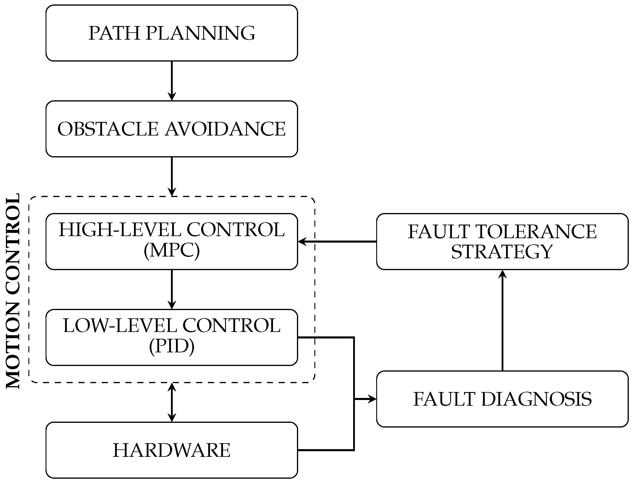
Figure 2.
Robotino representation,three-wheeled omnidirectional robot.
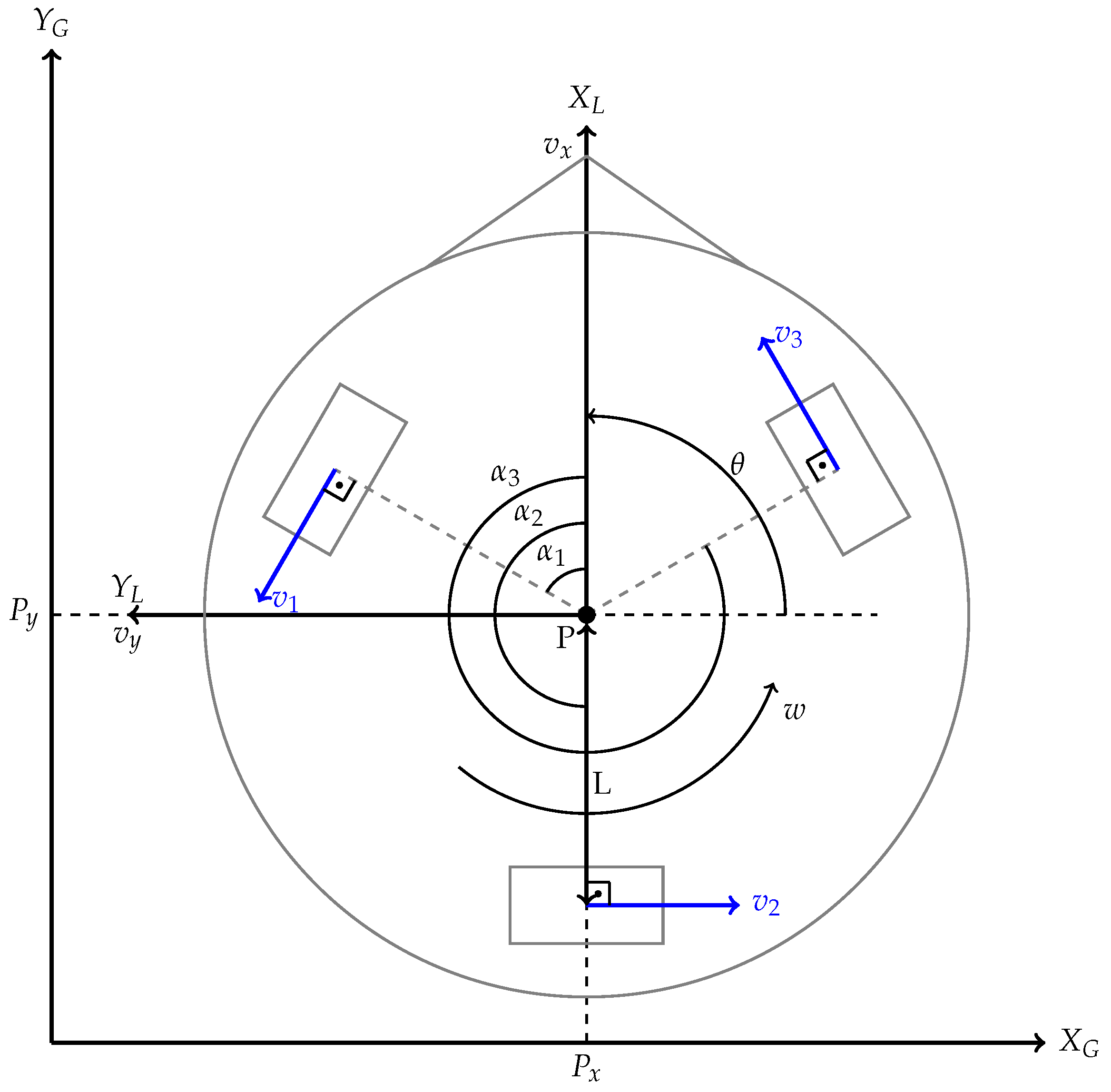
Figure 3.
Diagram block of control strategy.
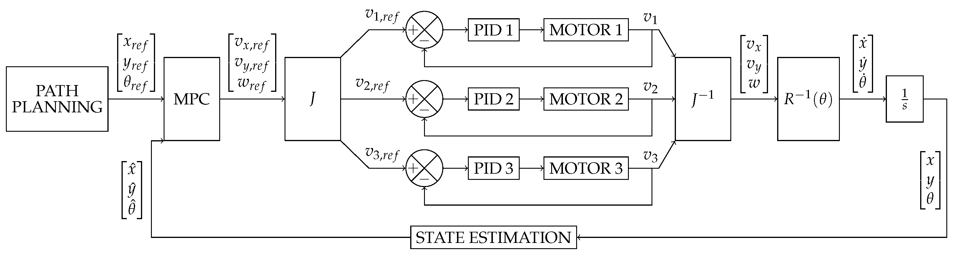
Figure 4.
Visual mark. The mobile robot approaches a table where a SCARA robot performs a pick-and-place task. The mobile robot then moves away from the table and navigates by following the markers it encounters along the way.
Figure 4.
Visual mark. The mobile robot approaches a table where a SCARA robot performs a pick-and-place task. The mobile robot then moves away from the table and navigates by following the markers it encounters along the way.
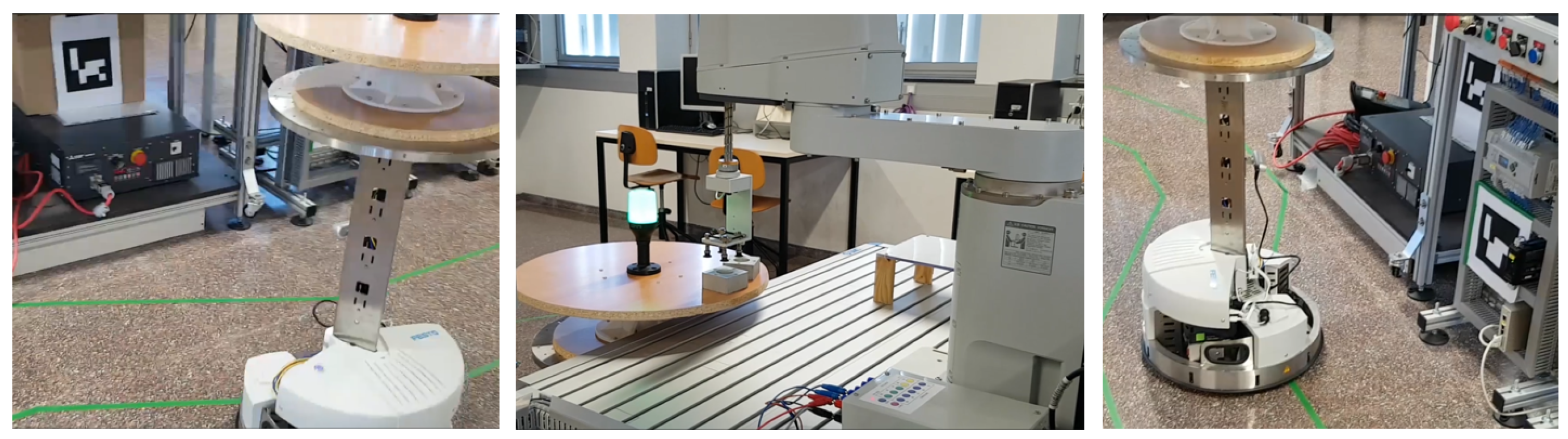
Figure 5.
(Left) PID motion control subprogram. (Right) Part of the sequential function chart.
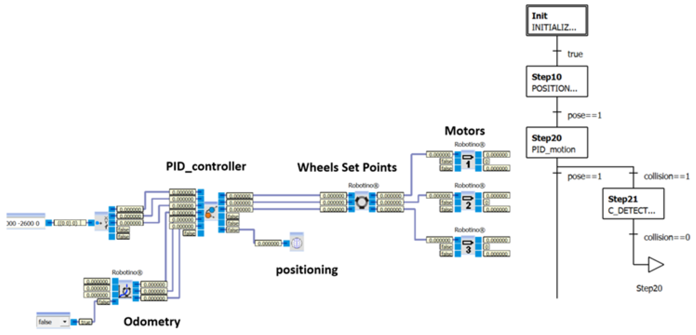
Figure 6.
(Left) The left Robotino stops in front of the right Robotino. (Right) The left Robotino follows the free navigation trajectory.
Figure 6.
(Left) The left Robotino stops in front of the right Robotino. (Right) The left Robotino follows the free navigation trajectory.
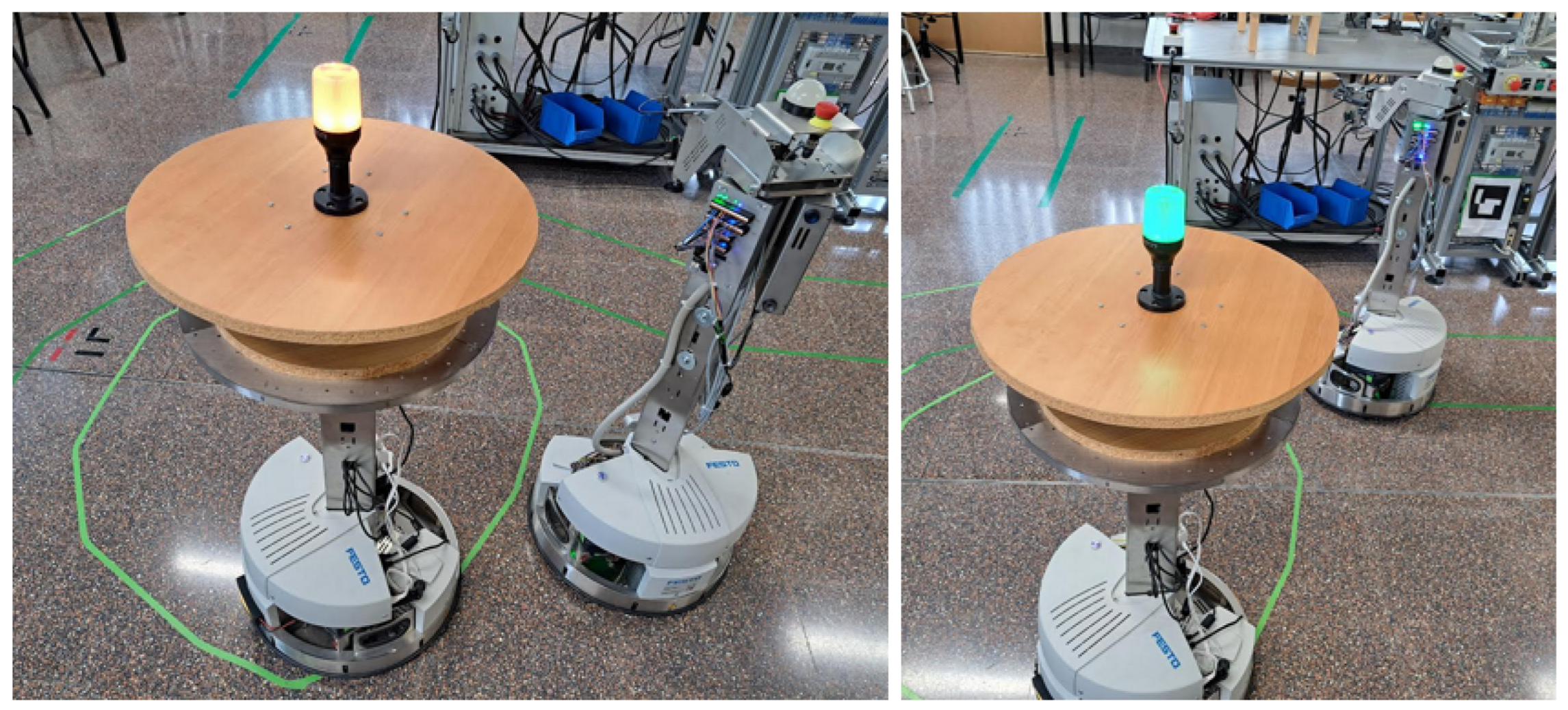
Figure 7.
Motor and PID identification results. The blue dashed line represents the velocity setpoint, the orange line shows the actual wheel velocity, and the green line corresponds to the identified first-order transfer function that describes the motor dynamics and PID controller response.
Figure 7.
Motor and PID identification results. The blue dashed line represents the velocity setpoint, the orange line shows the actual wheel velocity, and the green line corresponds to the identified first-order transfer function that describes the motor dynamics and PID controller response.
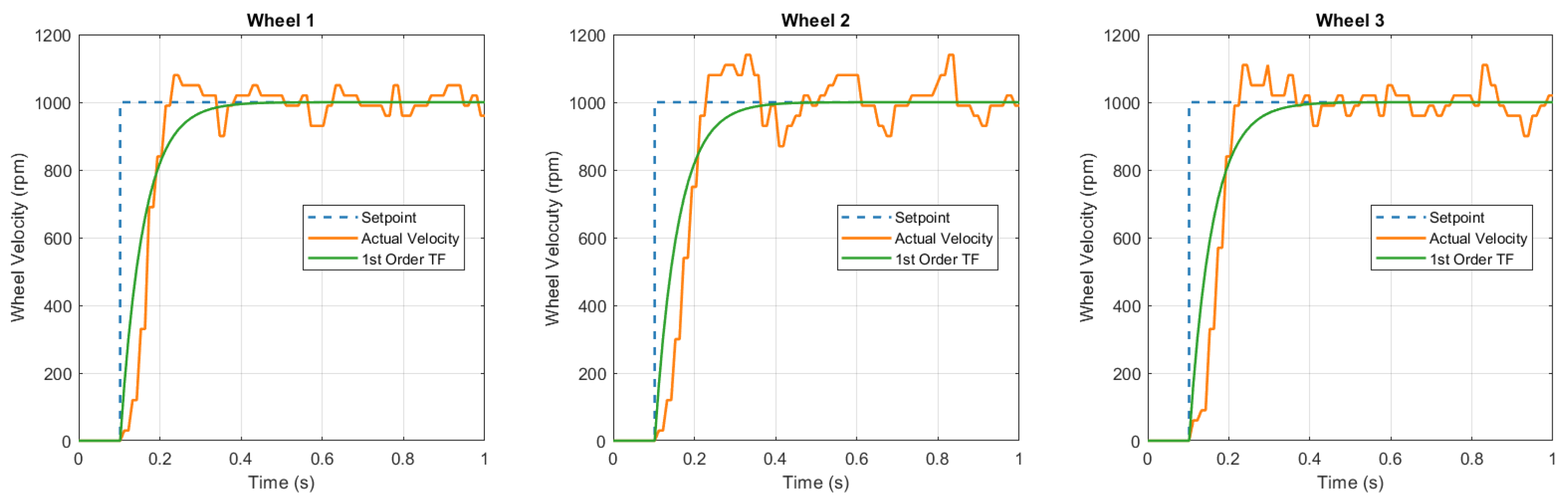
Figure 8.
Odometry results. The red dashed line represents the reference trajectory and the blue line the odometry data. The left plot shows the x and y position values, while the right plot illustrates the the orientation.
Figure 8.
Odometry results. The red dashed line represents the reference trajectory and the blue line the odometry data. The left plot shows the x and y position values, while the right plot illustrates the the orientation.
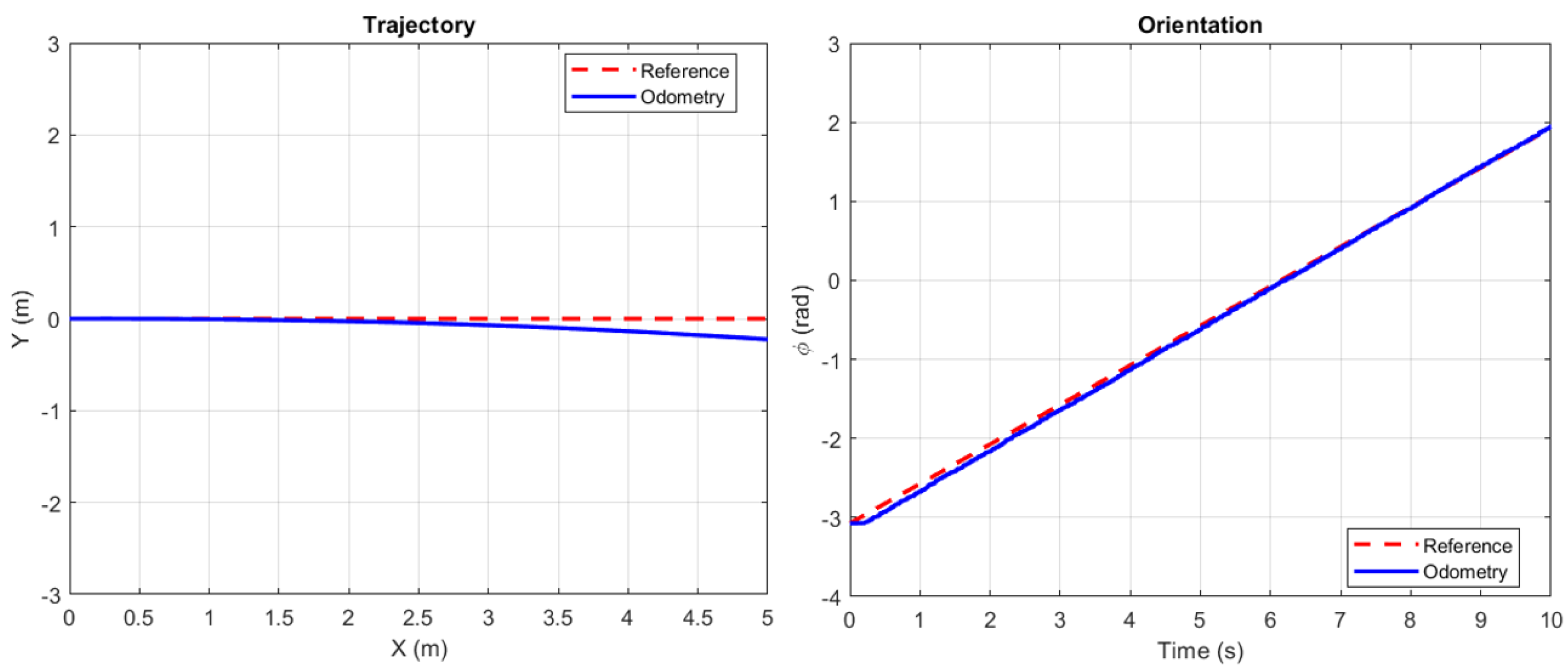
Figure 9.
Tracking performance of LPV-MPC following the lemniscate trajectory. The black dashed line represents the reference trajectory, and the red line corresponds to the LPV-MPC response.
Figure 9.
Tracking performance of LPV-MPC following the lemniscate trajectory. The black dashed line represents the reference trajectory, and the red line corresponds to the LPV-MPC response.
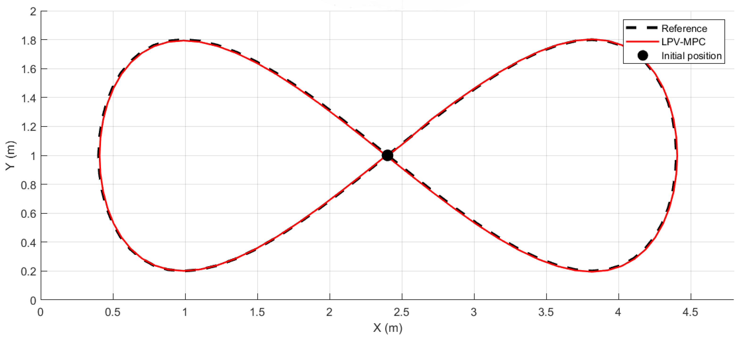
Figure 10.
Comparison between reference trajectory and the actual obtained using LPV-MPC for x, y and over time. The black dashed line represents the reference trajectory, and the red line corresponds to the LPV-MPC response.
Figure 10.
Comparison between reference trajectory and the actual obtained using LPV-MPC for x, y and over time. The black dashed line represents the reference trajectory, and the red line corresponds to the LPV-MPC response.
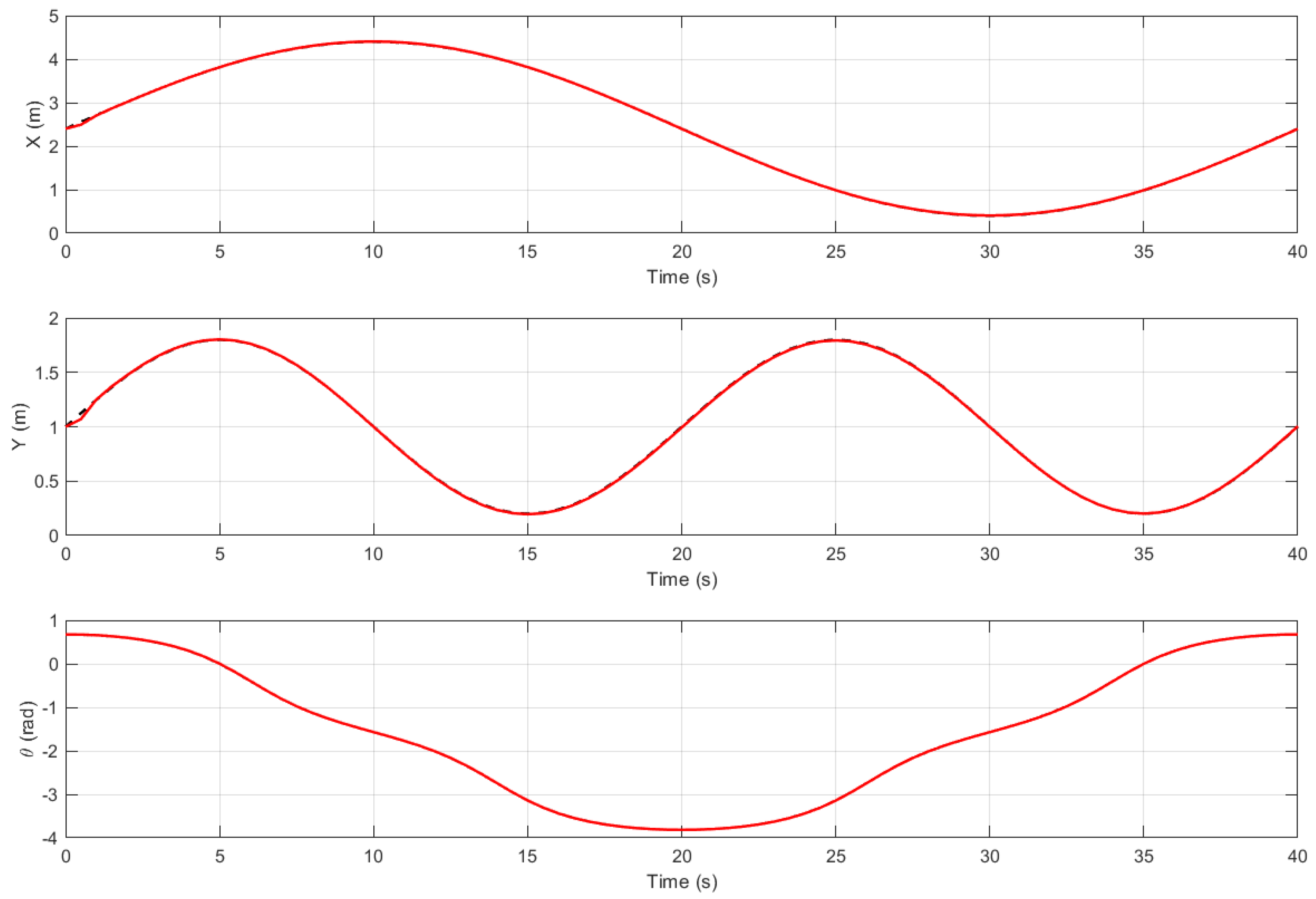
Figure 11.
Evaluation of the actuator performance. The reference wheel velocity (black dashed line) versus the actual wheel velocity (red solid line).
Figure 11.
Evaluation of the actuator performance. The reference wheel velocity (black dashed line) versus the actual wheel velocity (red solid line).
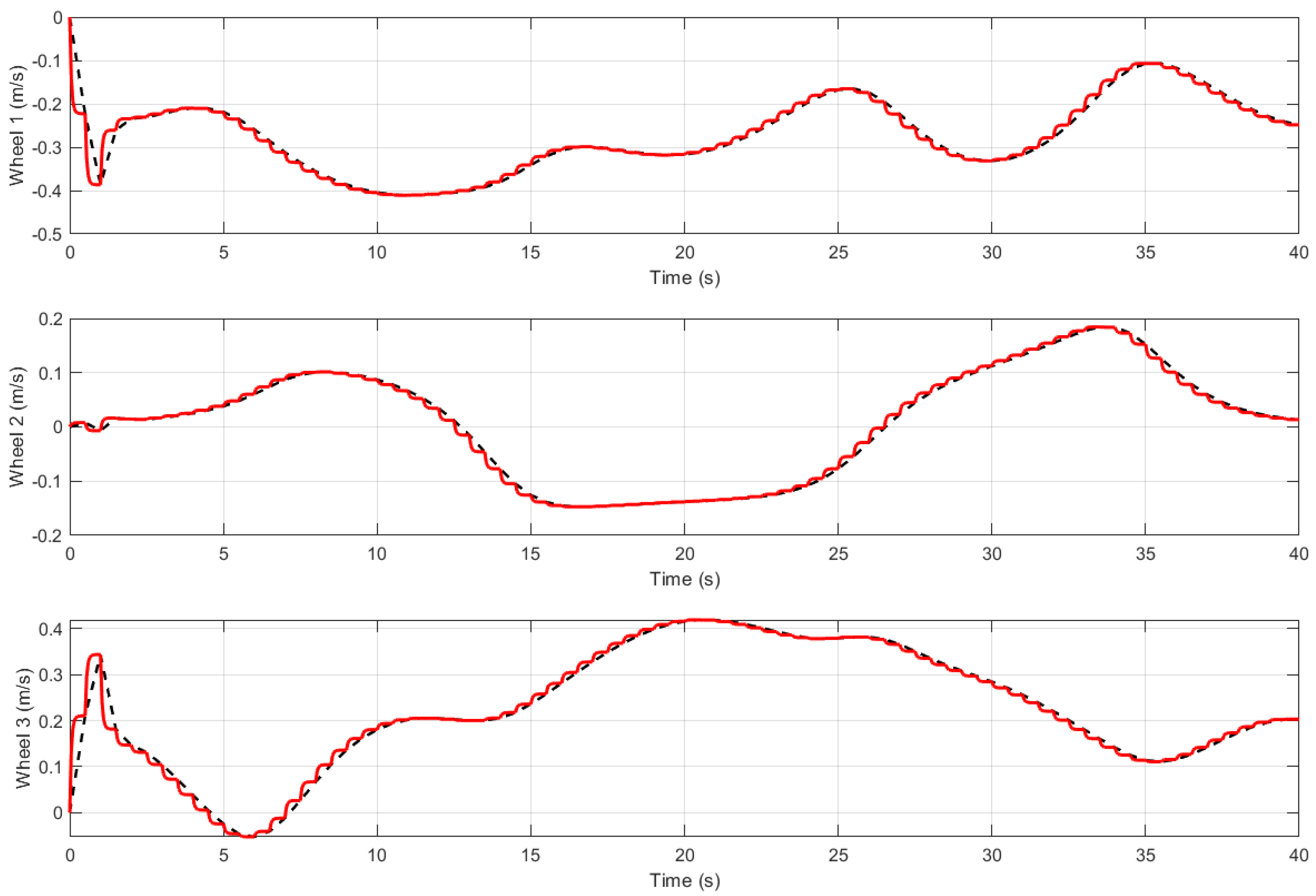
Figure 12.
Tracking errors in x, y, and over time. The red lines represents the error evolution in each state.
Figure 12.
Tracking errors in x, y, and over time. The red lines represents the error evolution in each state.
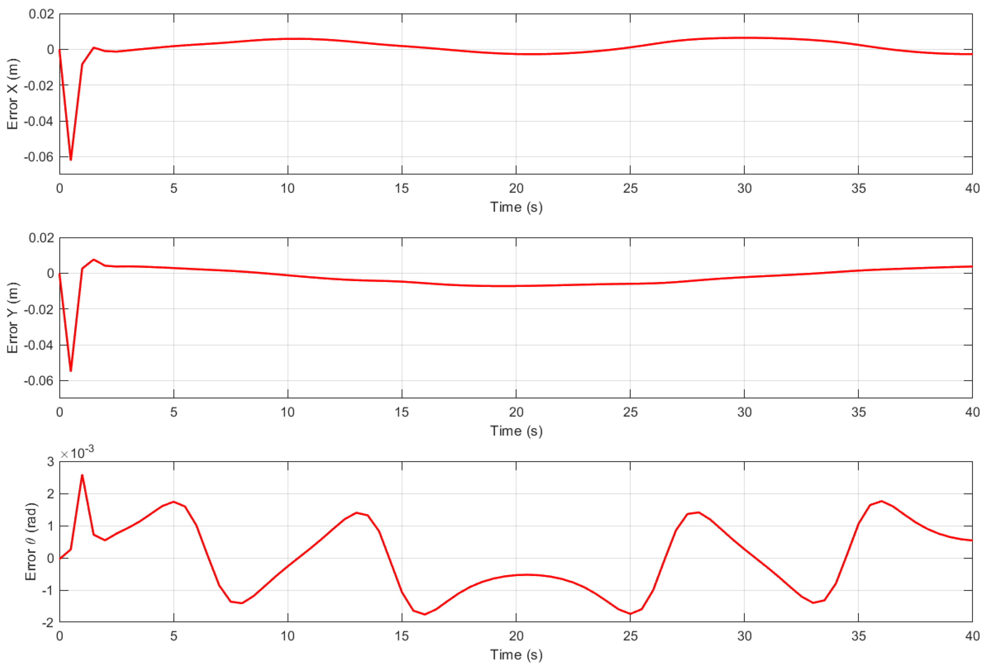

Table 1.
Examples of the use of Robotino.
| Authors | Control | Programming | Simulation |
|---|---|---|---|
| Niemueller et. al 2013 [7] | CLIPS Rule engine | ROS, C | Perception inputs |
| Mercorelli et. al 2017 [6] | Model Predictive Control | ROS | Simulink |
| Regier et. al 2020 [5] | Deep Reinforcement learning | ROS,Python | Gazebo |
| Rokhim et. al 2023 [4] | PID motion control | ROS | Gazebo |
Table 2.
Mean squared error for each state variable.
| State Variable | MSE Value |
|---|---|
| x (m) | |
| y (m) | |
| (rad) |
Disclaimer/Publisher’s Note: The statements, opinions and data contained in all publications are solely those of the individual author(s) and contributor(s) and not of MDPI and/or the editor(s). MDPI and/or the editor(s) disclaim responsibility for any injury to people or property resulting from any ideas, methods, instructions or products referred to in the content. |
© 2025 by the authors. Licensee MDPI, Basel, Switzerland. This article is an open access article distributed under the terms and conditions of the Creative Commons Attribution (CC BY) license (http://creativecommons.org/licenses/by/4.0/).
Copyright: This open access article is published under a Creative Commons CC BY 4.0 license, which permit the free download, distribution, and reuse, provided that the author and preprint are cited in any reuse.


