
Submitted:
09 April 2025
Posted:
12 April 2025
You are already at the latest version
Abstract
The bay-marsh boundary is a dynamic topographic feature. Advances in remote sensing provide cost-effective, high-resolution mapping technologies to detect change at fine scales. However, many questions remain about how to best apply these technologies and quantify change at bay-marsh boundaries. We combine UAS photogrammetry and boat-mounted echosounding to map the bay-marsh boundary over two consecutive years and use a previously collected Lidar dataset for decadal timescale comparisons. We evaluate accuracy, lateral and volumetric change rates, and how this approach compares to traditional methods of quantifying change. Results indicate an elevation uncertainty of 0.07 m for the topobathymetric DEMs. Volumetric erosion rates between marsh shorelines were -0.78 0.22 and -0.25 0.15 m3m-1yr-1 at an 8-year and annual sampling interval respectively. Lateral erosion rates were -1.57 0.15 and -1.54 0.07 m yr-1 at an 8-year and annual sampling interval respectively and were weakly correlated with volumetric change rates, even within morphologically similar sections of the marsh edge. Measured volumetric change rates of the marsh edge were reasonably estimated with limited vertical data at decadal timescales, suggesting that this change could be approximated with an RTK system. However, high-resolution mapping remains essential for assessing annual, event-driven, or small-scale change.
Keywords:
coastal change
; salt marsh
; drones
; echosounder
; photogrammetry
; structure-frommotion
; marsh retreat
; intertidal morphology
1. Introduction
Salt marshes provide a wide range of ecosystem services, such as nursery habitat for fishes and birds [1,2], improved water quality [3], carbon sequestration [4], and storm buffering [5]. The extent of salt marshes is inherently dynamic and cycles of progradation and retreat have been well documented. Contemporary salt marshes formed largely due to slowing rates of eustatic sea level rise (SLR) (<1 mm yr-1) in the late Holocene [6,7,8]. This stabilization of sea levels allowed for bay infilling that facilitated salt marsh expansion [9,10]. Accelerating rates of SLR and a decreased delivery of sediment to coastal systems, starting in the postindustrial period, has led to global losses of salt marsh area [11,12,13,14].
Considerable attention has been given to salt marsh adaptation to changing environmental conditions, particularly regarding vertical accretion to avoid drowning [15,16,17,18,19,20]. Salt marshes are also vulnerable to shoreline retreat, where wave-driven erosion of the marsh edge can result in rates of lateral retreat that commonly exceed 1 m yr-1 [9,21,22,23,24,25]. Thrust on the marsh scarp increases with increasing water level and wave height until the marsh is inundated and thrust rapidly decreases [23]. As such, moderate, yet frequent, storms account for the largest proportion of marsh retreat because the scarp of the marsh is often inundated during large storm surge events [24]. While SLR may increase marsh retreat rates due to increased water depths and wave heights [26], marsh land loss occurs independent of SLR when wave-driven marsh retreat is greater than sediment supply from rivers, tidal flats or offshore [14,27].
Conventionally, marsh shoreline erosion is quantified in terms of rates of lateral retreat of the marsh edge [25,28,29,30,31,32]. These assessments used data collected from RTK/total station surveys, erosion pins, or georeferenced aerial photography, together with moving boundary analysis to quantify rates of lateral change of marsh-edge position. A number of studies have found significant correlations between rates of lateral retreat and wave power at the marsh edge [28,29,33], while other studies have not [34]. McLoughlin et al. [29] found a stronger relationship between wave power and volumetric erosion rates than with lateral erosion rates along marsh shorelines, consistent with a dimensional analysis by Marani et al. [28] that argued that average incident wave energy flux, a measure of wave power, is proportional to volumetric erosion rate rather than the rate of linear retreat.
Some studies estimate volumetric erosion by multiplying lateral retreat rates by a representative height (e.g., scarp height). These volumetric approximations are constrained by limited vertical elevation data and assume that erosion is confined to the marsh shoreline (inner edge, Figure 1). However, a single vertical metric poorly represents the complex morphology of the marsh edge, and erosion may extend on- and off-shore of the inner edge to include the lower elevations of the intertidal marsh and the upper elevations of the intertidal flat (entire edge, Figure 1). A more comprehensive approach to quantifying volumetric marsh retreat involves resolving the 3-dimensional morphology of the bay-marsh boundary, including the shallow intertidal flat, over time and quantifying change across all morphodynamic zones.
Advancements in remote sensing, such as Structure-from-Motion (SfM) photogrammetry collected from an unoccupied aerial system (UAS), present cost-effective opportunities to map subaerial landscapes at high spatial and temporal resolutions that resolve detailed morphologies and detect fine-scale rates of change. These techniques have been widely applied to various landscapes for morphologic mapping [35,36,37,38,39] and have also been applied specifically to salt marshes, mainly to monitor ecological health [40,41,42,43]. Few of these studies have mapped the marsh edge, partially due to their motivations, and because of the logistical challenges of mapping in the lower intertidal. Vessel-based sidescan and multibeam sonar represent a comprehensive, yet expensive, solution to shallow water mapping [44,45]. Single-beam sonar sacrifices spatial coverage, but dramatically improves affordability and ease of use [44,46]. Within shallow bays, quantitative assessments of bathymetric change are only beginning to emerge as enough time has passed to facilitate detectable change [44].
A spatial gap in subaerial and subaqueous data is a common challenge in mapping land-water boundaries, creating whitespace (i.e., missing data) at the interface between the land and the water. At the bay-marsh boundary, whitespace might be eliminated by completing UAS SfM surveys during low tide and bathymetric surveys during high tide to establish overlap between datasets. Integrating mapping technologies in this way could increase the spatial and temporal resolution of morphologic mapping and improve our ability to quantify change. Still, many questions remain as to how best to apply these technologies to mapping and evaluating change at the bay-marsh boundary and how they compare to traditional methods.
Developing improved metrics of volumetric change at the bay-marsh boundary is central to understanding drivers of marsh retreat, forecasting future rates of marsh loss due to shoreline erosion, and constructing the sediment budgets necessary to characterize marsh resilience to changes in climate and land use [47]. However, assessments of volumetric change that resolve the complex morphology of the bay-marsh boundary do not exist. This study addresses this gap by repeatedly mapping the high resolution morphology of a bay-marsh boundary, quantifying change, and specifically addressing the following questions: (1) What spatial resolution and vertical accuracy can be achieved by combining UAS SfM and single-beam echosounding to map elevations across the bay-marsh boundary? (2) What is the contribution of various parts of the bay-marsh boundary to volumetric change? (3) Are lateral change rates correlated to volumetric change rates of the marsh edge? (4) What are the tradeoffs of mapping and quantifying change of the bay-marsh boundary at high resolutions compared to traditional methods? To answer these questions, we mapped the high-resolution morphology of a bay-marsh boundary using UAS SfM in combination with single-beam echosounding and constructed digital elevation models (DEMs) for two consecutive years. A Lidar dataset collected 8-years prior is used for longer-term comparisons. Morphodynamic change is quantified in terms of lateral and volumetric change rates and changes to cross-shore slope.
2. Methods
2.1. Site Description
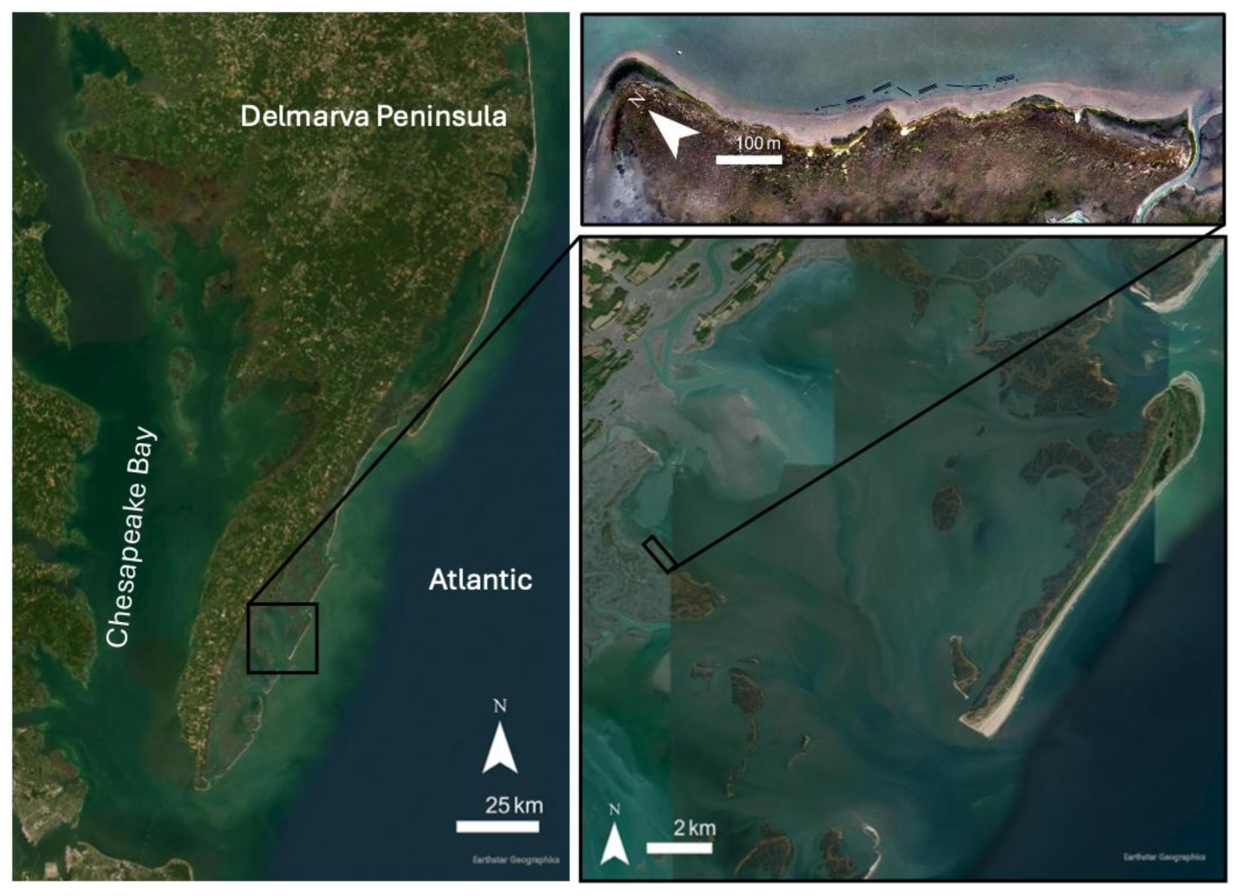
Hog Island Bay is located within the Volgenau Virginia Coast Reserve (hereafter the VCR), located on the Atlantic side and southern extent of the Delmarva Peninsula and part of the traditional territory and homelands of the Accomack people (Figure 2). The VCR is a near-wholly undeveloped coastal zone that includes 14 barrier islands protecting back-barrier bay-marsh systems, all of which vary in size and configuration. Small watersheds line the mainland, though none supply significant freshwater or sediment to the back-barrier system [48,49]. The primary external sediment source is sediment import from the coastal ocean during storms [50]. Agriculture dominates watershed land use, but runoff is sufficiently low to maintain excellent water quality in the back-barrier system [51]. SLR is 5.8 +/- 0.6 mm yr-1 at the nearest long-term tidal gauge [52]. The semidiurnal tides have a mean tidal range of 1.2 m [53]. About half of the bays are less than 1 m deep during mean low water, and areas deeper than a few meters are confined to large channels [54]. The highest magnitude winds that drive sediment resuspension tend to occur in the winter and approach from the SSE-SSW and N-NE [53]. Salt marsh vegetation in the intertidal marsh is dominated by Spartina alterniflora, with a mean stem height of 30 cm, though these heights are highly variable [53].
Short Prong Marsh (SP) is a mainland marsh in the southwest corner of Hog Island Bay that faces northeast (Figure 2). A portion of SP is protected by oyster reefs constructed in 2018, which can attenuate wave energy, depending on reef configuration and water level, and may influence morphodynamic change at the bay-marsh boundary [55]. Morphology of the marsh edge varies spatially. Generally, the northwest region of SP is prominently scarped. The scarp is less distinctive, but still present, in the central region, fronted by oyster reefs, and in the southwest region. Terraced features are scattered along the bay-marsh boundary a few meters offshore of the vegetation line. Maximum fetch is large (>9 km).
Figure 2.
Delmarva Peninsula (left), with closeups of Hog Island Bay (bottom right) and Short Prong Marsh (top right).
Figure 2.
Delmarva Peninsula (left), with closeups of Hog Island Bay (bottom right) and Short Prong Marsh (top right).
2.2. Data Collection
UAS flights were completed using a DJI Phantom 4 RTK drone to map the subaerial bay-marsh boundary using SfM. The DJI Ground Station RTK application was used for flight planning, allowing for automated piloting of an identical flight path each time a marsh was surveyed. Imagery was collected using a 20-megapixel camera with a 1-inch CMOS senor and a mechanical shutter that mitigates risk of rolling shutter blur. Flights were completed at an altitude of 100 m, providing a ground sample distance of approximately 3 cm. Photographic overlap was 80%. All UAS operations were completed in compliance with Federal Aviation Administration Part 107. Positioning was determined using two Emlid Reach RS2 GNSS RTK receivers with theoretical uncertainties of 7 mm +1 ppm in the horizontal and 14 mm +1 ppm in the vertical, meaning that the horizontal accuracy, for example, is 7 mm plus 1 mm per kilometer of distance from the base station. One receiver served as the base station and the other as a rover used to locate GCPs for SfM processing and provide ground-truth data along the marsh and intertidal flat to assess final DEM accuracy. Six acrylic GCPs along the marsh edge and intertidal flat were included in each survey (Figure 3). SfM data also used UAS onboard RTK and received corrections from the Emlid base station. A total of 276 ground-truth data points were collected including 110 on the vegetated marsh, 67 on the marsh shoreline, and 99 on the intertidal flat. All SfM surveys were completed during low tide to maximize exposure of the intertidal flat.
Echosounding data was collected using a CEESCOPE Hydrographic Survey System, featuring a boat-mounted transducer and an integrated NovAtel RTK GNSS receiver. The transducer employs a single-beam echosounder with a ping rate of 20 Hz and an accuracy up to 1 cm ± 0.1% of depth. All echosounding surveys were completed during high tide to maximize navigability of the bays and overlap with the SfM surveys. The echosounding survey pathway included 6 cross-shore transects spaced approximately 150 m apart and one alongshore transect near the marsh shoreline. SfM and echosounding surveys were completed in late summer of 2022 and 2023, following the same flight plan and survey path both years.
2.3. Data Processing
Agisoft Metashape Professional, version 1.8.4, was used to process UAS imagery using SfM [56]. First, imported images were aligned at the highest accuracy by approximating the camera position to create tie points as a sparse point cloud. GCPs were manually linked to their surveyed positions in no less than 10 photos. Sparse cloud filtering was completed through gradual selection, based on reconstruction uncertainty, projection accuracy, and reprojection error. A dense point cloud was created at the ultra-high quality setting and manually cleaned. Ground points were classified based on max angle (1°), max distance (0.05 m), cell size (2 m), and erosion radius (0 m) [57]. A DEM was created from the ground points as a regular grid and an orthomosaic was constructed from the seamless merging of the imagery. Surveys were processed using UAS onboard RTK and GCPs. Resulting orthomosaics and DEMs were exported to GIS and clipped to exclude all subaqueous areas.
Echosounding data was collected and processed using the Hydromagic hydrographic survey software by Eye4Software, which georeferences depths with RTK positioning to determine the position and elevation of each data point. The conversion of raw transducer data to depth depends on the speed of sound in water. A sensitivity test was completed to assess the effect of variations in salinity, pressure, and water temperature on sound velocity and depth. Salinity is relatively constant in the bays at 31 ppm (no significant terrestrial freshwater source). The effects of pressure on sounding velocity are negligible and considered constant. Daily temperature variations in the bay could have an influence over sound velocity, and therefore, depth. These variations were accounted for using water temperature data from the NOAA station at Wachapreague, VA (ID: 8631044; https://tidesandcurrents.noaa.gov).
2.4. Pre-exisiting Lidar Data
The USGS led an aerial Lidar survey in 2015, covering the entire Virginia portion of the Delmarva Peninsula [58]. The spatial extent of the dataset differs from marsh to marsh due to tidal variations, but includes the marsh edge in most areas, including SP. Vertical uncertainty of the DEM was tested with 113 checkpoints that were evenly distributed throughout the surveyed area, including non-vegetated terrain, such as bare earth, open terrain, and urban terrain, and vegetated terrain, such as forest, brush, tall weeds, crop, and high grass. Elevation uncertainty was calculated as the Root Mean Square Error (RMSE) between the DEM value at the checkpoint pixel and the surveyed elevation of the checkpoint at a 95% confidence level. The resulting bare-earth DEM has a resolution of 1 m and a vertical uncertainty of 12.2 cm. This dataset is leveraged as a baseline of comparison for this study.
2.5. Morphology and Morphodynamic Change
DEMs were generated to visualize morphology and evaluate morphodynamic change in terms of lateral shoreline change rates and volumetric change rates. SfM and Lidar DEMs were clipped to exclude all water. Processed soundings were imported into GIS and trimmed so that the spatial extent of the data points was approximately the same for both years to ensure that change comparisons between surveys represented measured change, rather than an effect of interpolation. The soundings were initially interpolated at a 5 m resolution using the natural neighbor method and were resampled to 0.03 m to retain the high resolution of the SfM DEMs when merging DEMs. The echosounding and SfM DEMs were stitched together using the Mosaic to New Raster tool in ArcGIS Pro to create seamless DEMs of the bay-marsh boundary for 2022 and 2023. The 2015 Lidar DEM has a 1 m resolution. The DEMs from UAS SfM were resampled to a 1 m resolution when compared to the Lidar DEM. The Minus (Spatial Analyst) tool was used to map elevation differences by subtracting DEM values of earlier DEMs from latter DEMs, such that negative values represent erosion and positive values represent deposition.
Metrics of morphodynamic change were evaluated for the entire alongshore length of the marsh (overall) and subdivided into three alongshore regions: the northwest region (NW), the central region fronted by oyster reefs (Reef), and the southeast region (SE). Temporal intervals between datasets allow for morphodynamic change comparisons at two timesteps, the 8-year timestep spanning 2015 to 2023 and the annual timestep from 2022 to 2023.
The marsh shoreline was determined for the SfM and Lidar datasets to measure lateral changes of the marsh edge. The marsh shoreline can be accurately identified as the vegetation line through imagery or as an abrupt elevation change through elevation data [59]. SfM datasets have the advantage of both imagery and elevation data. When marsh morphology exhibits complex features, like multiple abrupt elevation shifts (e.g., terraces), imagery is a useful tool for verifying the true shoreline, which generally corresponds to the vegetation line. The vegetation line of each orthomosaic was manually digitized in GIS for the SfM datasets. For the 2015 Lidar DEM, a slope map was generated using the Slope (Spatial Analyst) tool in ArcGIS Pro where the marsh scarp was identified as the maximum slope. The furthest onshore extent of the scarp was digitized as the shoreline. On- and off-shore baselines were manually drawn to approximate the general shape of the shorelines. Cross-shore transects were cast at 1 m intervals between the baselines and filtered using the Analyzing Moving Boundaries using R (AMBUR) software package to account for curvature of the shoreline [60]. Capture points were generated at the intersection of the transects and shorelines and then analyzed to calculate lateral change rates. The associated uncertainty is presented in the supplementary materials.
Cross-shore elevation profiles were created using the transects generated in AMBUR to visualize cross-sectional morphology, quantify elevation differences and volumetric change, and evaluate slope. Points were generated at 10 cm intervals along each transect, and elevations were extracted from each DEM at the location of each point. Transects and shorelines were overlain in GIS, intersection points were generated, and the distance from the intersection points to each transect point was calculated. For each point, the elevation difference was computed between 2015 and 2023 (8-year timestep) and 2022 and 2023 (annual timestep). Representative elevation profiles were generated for each year to visualize morphologic changes at the 8-year and annual timesteps for the marsh overall and by region. First, bins were created every 1 m across-shore for the 8-year timestep to match the resolution of the Lidar dataset and 0.1 m for the annual timestep to retain high-resolution for the SfM dataset. Elevations and elevation differences were averaged across transects within each bin and plotted with distance to the shoreline of the earlier dataset on the x axis (e.g., zeroed at the 2015 shoreline for the 8-year timestep, and 2022 for the annual timestep), providing representative elevation and elevation difference profiles for each region (Figure S1). Morphodynamic zones were distinguished where the inner edge is the area between marsh shorelines, the entire edge includes the inner edge and the erosional area that tapers on- and off-shore, and the intertidal flat begins at the offshore bound of the edge (Figure 1). The offshore bound of the intertidal flat was calculated as the mean offshore distance of the MLLW contour from the 2022 and 2023 DEMs. The intertidal flat for the 2015 Lidar dataset, and all comparisons at the 8-year timestep, represented a truncated intertidal flat because the Lidar data does not include the lower elevations of the intertidal flat. Volumetric change rates per alongshore length were calculated by averaging elevation differences within each morphodynamic zone for each transect, multiplying by the width of the zone, and dividing by the timestep.
2.5.1. Traditional Estimates of Volumetric Change
Two approaches were used to estimate volumetric change rates assuming limited access to vertical data, intended to approximate traditional methods for calculating volumetric change at the bay-marsh boundary. Given the wide availability of shoreline position data from RTK surveys or aerial photography, both approaches used the lateral shoreline change data described above, but differed in the way marsh edge height was approximated. Approach 1 assumed a uniform edge height derived from the representative elevation profiles by extracting the elevation of the top of the marsh edge and at the bottom of the marsh cliff. For approach 2, marsh edge height was measured every 30 meters alongshore using the transects generated during the AMBUR analysis. Elevations for edge height were extracted at points A-D in Figure 4 for each transect where elevations at A and B were taken at time 1 and C and D at time 2. The mean edge height between time 1 and time 2 was multiplied by lateral retreat of that transect to determine volumetric change. While approach 1 constrains the vertical component by a single approximation of marsh edge height, approach 2 approximates marsh edge height from measurements at intervals on the order of 10s of meters, a method that might be reasonable using RTK surveying.
2.6. Vertical Uncertainty
SfM DEMs, echosounder points, and ground-truth RTK points were used to assess elevation uncertainty () by calculating Root Mean Square Error ():
where is the number of data points, is the true value, and is the estimated value. Ground-truth RTK points were collected in 2023 and used as true values to calculate RMSE for the 2023 SfM DEM. Ideally, echosounder points would be validated against RTK points. However, collecting boat-mounted single-beam data creates major challenges in occupying the same location with handheld RTK. Instead, SfM data is used as the true value to calculate RMSE for echosounder points (estimated value) where the datasets overlap in the intertidal flat, similar to other works that use independent datasets to evaluate uncertainty of echosounder data [61]. The root square sum (RSS) was used to determine uncertainty associated with elevation differences ():
where and are the elevation uncertainties of the differenced datasets [62]. The cross-shore length scale () and timestep () were accounted for to evaluate uncertainty associated with volumetric change rates ():
3. Results
3.1. Elevation Uncertainty
[58]Elevation uncertainty () varied based on processing method and feature. In all cases, processing data with both onboard UAS RTK and GCPs provided the best agreement with ground-truth elevations. Overall, was low (0.07 m) (Table 1, Figure 5), including on the marsh (0.09 m) where it is often challenging to detect bare earth on the vegetated surface, even when using a point filtering protocol [40,43,57,63]. The shoreline (i.e., the top of the marsh cliff) had the highest of any feature (0.11 m), owing to its steep slope. The was lowest on the intertidal flat for both SfM and echosounder data (0.06 m).
3.2. Elevation Mapping and Profiles
Integration of SfM and echosounding mapping technologies facilitated the creation of seamless elevation maps from the lower intertidal marsh to the marsh cliff and into the subtidal flat for 2022 and 2023. Whitespace was eliminated by mapping the marsh and upper intertidal flat with UAS SFM at low tide and the entire intertidal flat through echosounding at high tide to create overlap in datasets between subaerial and subaqueous environments. Lidar alone was used to create the 2015 map, which therefore did not include the lower elevations of the intertidal flat.
DEMs from 2022 and 2023 resolve the detailed morphology of the bay-marsh boundary at a 0.3 m resolution (Figure 6). However, the lower intertidal flat morphology is derived from echosounding data, and while the DEM cell size remains 0.03 m, detail is only resolved to 5 m in the DEM. Elevation profiles (Figure 7) show a cross-sectional view of the bay-marsh boundary morphology, including the alongshore variability and elevation uncertainty. Profiles include the lower intertidal marsh, the steep marsh cliff, and the intertidal flat. The intertidal flat terminates 50 m offshore, but the profiles continue, showing 2022 and 2023 elevations meeting within millimeters. Data from 2015 does not extend to lower intertidal elevations because no bathymetric data was collected in conjunction with this large-scale Lidar mapping effort. The 2015 and 2022 profiles converge to within millimeters of each other in the intertidal flat.
3.3. Morphodynamic Change
Lateral change rates of the shoreline at SP were erosional over both timesteps and spatial variability was highest at the annual timestep (Figure 8, Table 2). Overall, the mean lateral change rates were -1.57 ± 0.15 m yr-1 for the 8-year timestep and -1.54 ± 0.07 m yr-1 for the annual timestep (Table 2). The rate of lateral erosion in the reef region significantly decreased from the 8-year (-1.61 ± 0.15 m yr-1) to the annual (-1.37 ± 0.07 m yr-1) timestep and was significantly less than annual rates in the NW (-1.55 ± 0.07 m yr-1) and SE (-1.70 ± 0.07 m yr-1).
Elevation difference profiles (Figure 9) allowed for the determination of morphodynamic zones (i.e., the entire edge, the inner edge, and the intertidal flat; Figure 1) for each region (Figure S1), and revealed a general pattern for a retreating bay-marsh boundary. The greatest magnitudes of erosion occurred within the inner edge (Figure 9). Erosion gradually decreased both on- and off-shore of the inner edge, defining the extent of the entire edge.
Mean volumetric change rates of the inner edge were significantly different at the 8-year timestep compared to the annual timestep (-0.78 ± 0.22 m3 m-1 yr-1 and -0.25 ± 0.15 m3 m-1 yr-1 respectively) (Figure 10 and Table 3). Mean volumetric change rates of the entire edge were not significantly different between timesteps (-0.88 ± 0.42 m3 m-1 yr-1 at the 8-year timestep and -0.49 ± 0.60 m3 m-1 yr-1 at the annual timestep). The standard deviation and the interquartile ranges were similar from the inner edge to the entire edge at the 8-year timestep and increased from the inner edge to the entire edge for the annual timestep. This suggests increased spatial variability of volumetric change rates of the erosional area outside the inner edge, herein referred to as the fringe edge, at the annual timestep.
Variations in lateral change rates by region were relatively small at the 8-year timestep, ranging from -1.53 ± 0.15 m yr-1 in the SE to -1.61 ± 0.15 m yr-1 in the reef region (Table 2). However, volumetric change rates across the inner edge ranged from -0.45 ± 0.21 m3 m-1 yr-1 in the SE to -1.00 ± 0.24 m3 m-1 yr-1 in the reef region at the 8-year timestep (Table 3). Volumetric change rates were lowest in the SE region at the annual timestep (-0.08 ± 0.15 m3 m-1 yr-1), despite a lateral change rate of -1.70 ± 0.07 m yr-1. Lateral change rates were weakly correlated (0.25 < r < 0.5) to volumetric change rates at both timesteps for each region, except at the annual timestep in the SE where the relationship was not significant (Figure S3). This suggests that high lateral change rates do not necessarily imply high volumetric change rates.
Elevation changes across the intertidal flat and the truncated flat were consistently positive, but within the margin of error for both timesteps (Figure 9). However, closure of the 2022 and 2023 elevation profiles near and beyond MLLW suggests that uncertainty may be smaller than the indicated values (Figure 7). Deposition in the intertidal flat could be anticipated due to the redistribution of sediment eroded from the marsh edge. On longer timescales, deposition on the intertidal flat would be necessary for the flat to maintain its elevation relative to mean water level as sea level rises.
3.3.1. Traditional Estimates of Volumetric Change
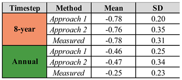
Volumetric change rates were estimated for the entire edge using a uniform measurement of marsh edge height for approach 1 and a spatially varied measurement for approach 2 (Figure 11 and Table 4). For the 8-year timestep, estimates of mean volumetric change rates were -0.78 and -0.76 m3 m-1 yr-1 for approach 1 and 2 respectively, providing a good estimate of the measured mean of the inner edge (-0.78 ± 0.22 m3 m-1 yr-1). Approach 1 poorly represents the distribution of volumetric change rates along the marsh edge while approach 2 represents the measured distribution reasonably well (Figure 11). The mean volumetric change rates were -0.46 and -0.47 m3 m-1 yr-1 for approach 1 and 2 respectively at the annual timestep, compared to the measured mean of -0.25 ± 0.15 m3 m-1 yr-1. Neither approach provided a good estimate of the measured mean or representation of the measured distribution at the annual timestep.
4. Discussion
4.1. Elevation Uncertainty
Vertical accuracy of SfM DEMs was greatest when using both onboard UAS RTK and multiple GCPs deployed across the site. Further testing of UAS RTK is needed to reduce reliance on GCPs for georeferencing. In our experience, substantial positioning offsets sometimes occurred when mixing products from different manufacturers of the base and rover for RTK surveying regardless of the baseline distance. Consequently, we used an Emlid base and rover to survey GCPs. However, the Emlid also served as the base for the DJI UAS RTK. It is unknown if using a DJI base would improve the UAS RTK. At its best, UAS RTK provides instantaneous solutions for each position. Using GCPs alone provides fewer positioning measurements (limited by the number of GCPs rather than photos taken) but has the advantage of averaging many solutions when surveying each GCP. GCPs can also be used as check points, or ground-truth points, to assess SfM accuracy. While surveying without GCPs would reduce labor, some amount of ground control is necessary to assess accuracy and verify validity of the data.
The low uncertainty observed on the intertidal flat (0.06 m) is likely due to the lack of both vegetation and steep morphologic features. Unless prominent pooling of water is present, the intertidal flat is an excellent surface for SfM at low tide. Dense vegetation increases error on the marsh because SfM constructs surfaces based online-of-sight in photographs. This was mitigated through point cloud filtering to distinguish bare earth from vegetation points. Elevation uncertainty on the marsh was 0.09 m, a low value compared to other studies where marsh elevation uncertainty using SfM ranges from 0.17-1 m [64,65,66], suggesting that the point cloud filtering was successful and vegetation was not prohibitively dense. For detecting the shoreline, ground-truth measurements were taken on top of the marsh scarp while DEM-derived values relied on digital extraction of the shoreline and may select an elevation lower on the scarp. Excellent agreement was observed between SfM and echosounder data near the marsh-flat border (Table 1), validating the mapping of morphology across the bay-marsh boundary by surveying the marsh and upper elevations of the intertidal flat during low tide using UAS SfM and the intertidal flat during high tide using echosounding. This result also supports a new method of validating boat-mounted echosounding data by creating overlap with UAS SfM.
4.2. Morphodynamic Change
Combining mapping techniques allowed us to construct high-resolution DEMs of the marsh-bay boundary. We differenced DEMS collected one year and 8 years apart to quantify volumetric change rates across different morphodynamic zones of the marsh edge. Whether those differences in volumetric change rates are significant is dependent on the temporal change in elevation values and their uncertainty. Uncertainty associated with volumetric change rates is a function of the combined uncertainty of the DEMs and the cross-shore length scale over which change is measured (equation 3). Our analysis indicated an overall elevation uncertainty of 0.07 m, however, closure of our measured elevation profiles to within a few millimeters on the marsh platform and near and beyond MLLW (Figure 7) suggests that there was no offset between datasets and that the uncertainty may be smaller.
Marshes in our study area lost 0.5 – 1.0 m3 m-1 yr-1 across their entire edge over the 8-year interval from 2015 – 2023. Volumetric erosion rates for the inner edge were 3 times greater at the 8-year timestep compared to the annual timestep, potentially reflecting a high level of interannual variability that averages out on decadal timescales. However, volumetric change rates for the entire edge did not differ significantly by timestep or from inner edge rates owing to the large uncertainty in erosion rates for the fringe edge. The fringe edge contributed approximately 50% of the volumetric erosion rate to the entire edge at the annual timestep and only 12% at the 8-year timestep, suggesting that the width of the fringe edge does not scale with time and may remain relatively constant. Given the mean volumetric erosion rate of the inner edge at the annual timestep (-0.25 m³ m⁻¹ yr⁻¹) and a constant contribution from the fringe edge (-0.24 m³ m⁻¹), after 10 years the fringe edge would account for less than 10% of total volumetric erosion, indicating that the contribution of the fringe edge to volumetric erosion becomes relatively unimportant on decadal time scales.
Previous studies found that most marsh retreat was caused by moderate storms with a 2.5 month return period because the marsh edge tends to be inundated and protected from wave attack during larger storm surge events [67]. While retreat rates may be expected to respond to changes in the return period of moderate storms, our results show that rates of marsh lateral retreat have been approximately constant over the time interval of our study (8 years), consistent with other studies that have found nearly constant retreat rates over multiple decades [68]. Volumetric change rates were more variable spatially and temporally.
High lateral change rates in the SE region at the annual timestep were observed due to retreat of the vegetation line (Figure 8 and Table 2). However, volumetric change rates were negligible due to little change in elevation (Figure 10 and Table 3). Overall, lateral change rates were only weakly correlated to volumetric change rates along the entire marsh edge (Figure S3). These findings suggest that alongshore variations in volumetric change rates are not necessarily proportional to lateral change rates, and that sometimes high lateral change of the vegetation line may occur despite little volumetric change. This weak relationship between lateral and volumetric change highlights the necessity of measuring volumetric change when quantifying marsh loss/gain contributions to sediment budgets.
Elevation changes on the intertidal flat did not exceed the margin of error. A marsh edge volumetric erosion rate of 0.5 m3 m-1 yr-1, representative of our results (Table 3), spread over the intertidal flat (50 m) and the marsh platform fringe (~ 30 m) would create an annual deposit thickness on the order of 6 mm, indicating it would take over a decade to create a measurable change in flat elevation. Future work might refine change measurements in the intertidal flat with an in situ approach that measures relative change with the precision necessary to confidently detect millimeter- to centimeter-scale change or allow for multiple decades between measurements. Elevation measurements that extend onto the intertidal flat are valuable, not only for quantifying change within the flat, but also for measuring change across the marsh edge. As the timestep between surveys increases, the most recent survey needs to extend at least to the intertidal flat of the baseline survey to measure change of the marsh edge completely. Excluding intertidal flat data could result in missing contributions from the offshore area of the edge to volumetric change rates.
4.3. Comparisons to traditional metrics
Traditional methods of assessing marsh retreat usually measure lateral change of the marsh shoreline from historical imagery. However, volumetric change is needed for sediment budgeting and has been correlated to wave energy [28,68], even with limited vertical data. Two approaches for estimating volumetric change rates with limited vertical data were compared to measurements made from high-resolution DEMs. The mean, spatial variability, and overall distribution of volumetric change rates of the inner edge were reasonably well estimated using a spatially varying edge height (approach 2) at the 8-year timestep (Figure 11, Table 4), suggesting that volumetric change could be estimated at decadal timescales with limited vertical data. In practice, approach 2 involves measuring the elevation of the top of the marsh edge, the elevation of the marsh toe just offshore of the marsh cliff or shoreline, and the elevation of the marsh toe or tidal flat near the approximate location of the previous marsh shoreline. In this example, these measurements are taken every 30 meters alongshore, a reasonable task with an RTK system depending on the scale.
4.4. Oyster Reefs
The oyster reefs that front a portion of the SP marsh edge were constructed in 2018 and provide the opportunity to highlight the value of mapping and quantifying change at a high-resolution along the bay-marsh boundary. Constructed oyster reefs can attenuate wave energy at the bay-marsh boundary [55], which could mitigate marsh retreat. The baseline survey for the 8-year timestep was conducted in 2015, 3 years prior to oyster reef installment, and the annual timestep represents surveys from 2022 and 2023, 4 and 5 years post-installment respectively. There was no significant difference between 8-year and annual timestep lateral change rates for the NW and SE regions (Figure 8). However, lateral retreat rates of the reef region at SP were significantly reduced from -1.61 ± 0.15 m yr-1 at the 8-year timestep to -1.37 ± 0.07 m yr-1 at the annual timestep, likely due to a reduction in wave attack from the oyster reefs. Maximum slope of the marsh edge decreased over time for the reef region and increased over time for the NW and SE region (Figure S4, Table S2). An intertidal flat contour was used to approximate the marsh toe in 2015 and 2022 (Figure 12). Erosion of the marsh toe was observed in the NW and SE regions while the marsh toe was stable in the reef region (Figure 12). Although the top of the marsh scarp in the reef region continued to retreat, resulting in significantly erosional lateral and volumetric change rates, the stabilization of the marsh toe promoted an elongation of the reef-fronted bay-marsh boundary, similar to findings from previous work [69]. This analysis demonstrates the values of repeat high-resolution mapping to detect small-scale change due to human intervention.
5. Conclusions
The detailed morphology of a bay-marsh boundary was mapped for two consecutive years using a combination of UAS SfM and boat-mounted echosounding, with a resolution of 0.03 m and a vertical uncertainty of 0.07 m. A Lidar dataset collected 8 years prior was used to assess changes over decadal timescales. Erosion was measured between marsh shorelines (the inner edge), with volumetric change rates of -0.78 ± 0.22 m3 m-1 yr-1 at the 8-year timestep and -0.25 ±0.15 m3 m-1 yr-1 at the annual timestep. Lateral change rates were -1.57 ± 0.15 m yr-1 for the 8-year timestep and -1.54 ± 0.07 m yr-1 for the annual timestep. High lateral change rates were measured in a section of the marsh (SE), despite little volumetric change. Lateral and volumetric change rates were only weakly correlated along the marsh edge, emphasizing the importance of volumetric measurements when quantifying marsh retreat. Volumetric change rates were well estimated at the decadal timescale with limited vertical data, suggesting that RTK surveys, measuring elevations of the top and bottom of the marsh cliff and the intertidal flat at intervals on the order of 10s of meters, could be used to determine volumetric change of the marsh edge. This approach may be particularly valuable and efficient when the objective is to monitor volumetric retreat because resolving the high-resolution morphology of the bay-marsh boundary may be cost- or skill-prohibitive. A higher resolution mapping approach is valuable for evaluating change across the entire bay-marsh boundary at finer scales, making it particularly useful for assessing annual or event-driven changes, as well as changes at small spatial scales.
Author Contributions
Conceptualization, T.B. and P.W.; methodology, T.B. and P.W.; software, T.B; validation, T.B.; formal analysis, T.B.; investigation, T.B. and P.W.; resources, P.W.; data curation, T.B.; writing—original draft preparation, T.B.; writing—review and editing, T.B. and P.W.; visualization, T.B.; supervision, P.W.; project administration, P.W.; funding acquisition, P.W. All authors have read and agreed to the published version of the manuscript.
Funding
This research was funded by the National Science Foundation (NSF), through the VCR LTER award 1832221.
Data Availability Statement
The original data presented in the study are openly available in the Environmental Data Initiative at https://doi.org/10.6073/pasta/537d876206a554a58f988499177401bd.
Acknowledgments
Logistical and field work support was provided by the staff and facilities at the Anheuser-Busch Coastal Research Center. We would like to thank Michael Cornish for advising on UAV operation and data processing, and Max Castorani and David Carr for statistical support.
Conflicts of Interest
The authors declare no conflicts of interest.
Abbreviations
The following abbreviations are used in this manuscript:
| SLR | Sea Level Rise |
| MLLW | Mean Lower Low Water |
| SfM | Structure-from-Motion |
| UAS | Unoccupied Aerial System |
| DEM | Digital Elevation Model |
| VCR | Volgenau Virginia Coast Reserve |
| SP | Short Prong Marsh |
| AMBUR | Analyzing Moving Boundaries Using R |
| Elevation Uncertainty | |
| RMSE | Root Mean Square Error |
| RSS | Root Square Sum |
| Elevation Difference Uncertainty | |
| Volumetric Change Rate Uncertainty | |
| SD | Standard Deviation |
References
- Minello, T.J.; Able, K.W.; Weinstein, M.P.; Hays, C.G. Salt Marshes as Nurseries for Nekton: Testing Hypotheses on Density, Growth and Survival through Meta-Analysis. Mar Ecol Prog Ser 2003, 246, 39–59. [Google Scholar] [CrossRef]
- Gjerdrum, C.; Elphick, C.S.; Rubega, M. Nest Site Selection and Nesting Success in Saltmarsh Breeding Sparrows: The Importance of Nest Habitat, Timing, and Study Site Differences. Condor 2005, 107, 849. [Google Scholar] [CrossRef]
- Cui, B.; Yang, Q.; Yang, Z.; Zhang, K. Evaluating the Ecological Performance of Wetland Restoration in the Yellow River Delta, China. Ecol Eng 2009, 35, 1090–1103. [Google Scholar] [CrossRef]
- McLeod, E.; Chmura, G.L.; Bouillon, S.; Salm, R.; Björk, M.; Duarte, C.M.; Lovelock, C.E.; Schlesinger, W.H.; Silliman, B.R. A Blueprint for Blue Carbon: Toward an Improved Understanding of the Role of Vegetated Coastal Habitats in Sequestering CO2. Front Ecol Environ 2011, 9, 552–560. [Google Scholar] [CrossRef]
- Möller, I.; Spencer, T.; French, J.R.; Leggett, D.J.; Dixon, M. Wave Transformation over Salt Marshes: A Field and Numerical Modelling Study from North Norfolk, England. Estuar Coast Shelf Sci 1999, 49, 411–426. [Google Scholar] [CrossRef]
- Donnelly, J.P. A Revised Late Holocene Sea-Level Record for Northern Massachusetts, USA. J Coast Res 2006, 22, 1051–1061. [Google Scholar] [CrossRef]
- Engelhart, S.E.; Horton, B.P. Holocene Sea Level Database for the Atlantic Coast of the United States. Quat Sci Rev 2012, 54, 12–25. [Google Scholar] [CrossRef]
- Hein, C.J.; Fitzgerald, D.M.; Cleary, W.J.; Albernaz, M.B.; De Menezes, J.T.; Klein, A.H. da F. Evidence for a Transgressive Barrier within a Regressive Strandplain System: Implications for Complex Coastal Response to Environmental Change. Sedimentology 2013, 60, 469–502. [Google Scholar] [CrossRef]
- Fagherazzi, S.; Kirwan, M.L.; Mudd, S.M.; Guntenspergen, G.R.; Temmerman, S.; D’Alpaos, A.; Van De Koppel, J.; Rybczyk, J.M.; Reyes, E.; Craft, C.; et al. Numerical Models of Salt Marsh Evolution: Ecological, Geomorphic, and Climatic Factors. Reviews of Geophysics 2012, 50, 1–28. [Google Scholar] [CrossRef]
- Oertel, G.F.; Kraft, J.C. New Jersey and Delmarva Barrier Islands. In Geology of Holocene Barrier Island Systems; Davis, R.A., Ed.; Springer, Berlin, Heidelberg, 1994.
- Campbell, A.D.; Fatoyinbo, L.; Goldberg, L.; Lagomasino, D. Global Hotspots of Salt Marsh Change and Carbon Emissions. Nature 2022, 612, 701–706. [Google Scholar] [CrossRef]
- Nicholls, R.J.; Hoozemans, F.M.J.; Marchand, M. Increasing Flood Risk and Wetland Losses Due to Global Sea-Level Rise: Regional and Global Analyses. Global Environmental Change 1999, 9. [Google Scholar] [CrossRef]
- Weston, N.B. Declining Sediments and Rising Seas: An Unfortunate Convergence for Tidal Wetlands. Estuaries and Coasts 2014, 37, 1–23. [Google Scholar] [CrossRef]
- Mariotti, G.; Fagherazzi, S. Critical Width of Tidal Flats Triggers Marsh Collapse in the Absence of Sea-Level Rise. Proceedings of the National Academy of Sciences 2013, 110, 5353–5356. [Google Scholar] [CrossRef]
- Kirwan, M.L.; Walters, D.C.; Reay, W.G.; Carr, J.A. Sea Level Driven Marsh Expansion in a Coupled Model of Marsh Erosion and Migration. Geophys Res Lett 2016, 43, 4366–4373. [Google Scholar] [CrossRef]
- Breithaupt, J.L.; Smoak, J.M.; Byrne, R.H.; Waters, M.N.; Moyer, R.P.; Sanders, C.J. Avoiding Timescale Bias in Assessments of Coastal Wetland Vertical Change. Limnol Oceanogr 2018, 63, S477–S495. [Google Scholar] [CrossRef] [PubMed]
- Sommerfield, C.K. On Sediment Accumulation Rates and Stratigraphic Completeness: Lessons from Holocene Ocean Margins. Cont Shelf Res 2006, 26, 2225–2240. [Google Scholar] [CrossRef]
- Kirwan, M.L.; Temmerman, S.; Guntenspergen, G.R.; Fagherazzi, S. Reply to “Marsh Vulnerability to Sea-Level Rise”. Nat Clim Chang 2017, 7, 756–757. [Google Scholar] [CrossRef]
- Day, J.W.; Scarton, F.; Rismondo, A.; Are, D. Rapid Deterioration of a Salt Marsh in Venice Lagoon, Italy. J Coast Res 1998, 14, 583–590. [Google Scholar]
- Blum, L.K.; Christian, R.R.; Cahoon, D.R.; Wiberg, P.L. Processes Influencing Marsh Elevation Change in Low- and High-Elevation Zones of a Temperate Salt Marsh. Estuaries and Coasts 2021, 44, 818–833. [Google Scholar] [CrossRef]
- Marani, M.; D’Alpaos, A.; Lanzoni, S.; Santalucia, M. Understanding and Predicting Wave Erosion of Marsh Edges. Geophys Res Lett 2011, 38, 1–5. [Google Scholar] [CrossRef]
- McLoughlin, S.M.; Wiberg, P.L.; Safak, I.; McGlathery, K.J. Rates and Forcing of Marsh Edge Erosion in a Shallow Coastal Bay. Estuaries and Coasts 2015, 38, 620–638. [Google Scholar] [CrossRef]
- Tonelli, M.; Fagherazzi, S.; Petti, M. Modeling Wave Impact on Salt Marsh Boundaries. J Geophys Res Oceans 2010, 115, 1–17. [Google Scholar] [CrossRef]
- Leonardi, N.; Ganju, N.K.; Fagherazzi, S. A Linear Relationship between Wave Power and Erosion Determines Salt-Marsh Resilience to Violent Storms and Hurricanes. Proc Natl Acad Sci U S A 2016, 113, 64–68. [Google Scholar] [CrossRef]
- Priestas, A.M.; Mariotti, G.; Leonardi, N.; Fagherazzi, S. Coupled Wave Energy and Erosion Dynamics along a Salt Marsh Boundary, Hog Island Bay, Virginia, USA. J Mar Sci Eng 2015, 3, 1041–1065. [Google Scholar] [CrossRef]
- Mariotti, G.; Fagherazzi, S.; Wiberg, P.L.; McGlathery, K.J.; Carniello, L.; Defina, A. Influence of Storm Surges and Sea Level on Shallow Tidal Basin Erosive Processes. J Geophys Res Oceans 2010, 115, 1–17. [Google Scholar] [CrossRef]
- Fagherazzi, S.; Mariotti, G.; Wiberg, P.L.; McGlathery, K.J. Marsh Collapse Does Not Require Sea Level Rise. Oceanography 2013, 26, 70–77. [Google Scholar] [CrossRef]
- Marani, M.; D’Alpaos, A.; Lanzoni, S.; Santalucia, M. Understanding and Predicting Wave Erosion of Marsh Edges. Geophys Res Lett 2011, 38. [Google Scholar] [CrossRef]
- McLoughlin, S.M.; Wiberg, P.L.; Safak, I.; McGlathery, K.J. Rates and Forcing of Marsh Edge Erosion in a Shallow Coastal Bay. Estuaries and Coasts 2015, 38, 620–638. [Google Scholar] [CrossRef]
- Cadigan, J.A.; Jafari, N.H.; Wang, N.; Chen, Q.; Zhu, L.; Harris, B.D.; Ding, Y. Near-Continuous Monitoring of a Coastal Salt Marsh Margin: Implications for Predicting Marsh Edge Erosion. Earth Surf Process Landf 2023, 48, 1362–1373. [Google Scholar] [CrossRef]
- Leonardi, N.; Fagherazzi, S. Effect of Local Variability in Erosional Resistance on Large-Scale Morphodynamic Response of Salt Marshes to Wind Waves and Extreme Events. Geophys Res Lett 2015, 42, 5872–5879. [Google Scholar] [CrossRef]
- Schwimmer, R.A. Rates and Processes of Marsh Shoreline Erosion in Rehoboth Bay, Delaware, U.S.A. J Coast Res 2001, 17, 672–683. [Google Scholar]
- Leonardi, N.; Ganju, N.K.; Fagherazzi, S. A Linear Relationship between Wave Power and Erosion Determines Salt-Marsh Resilience to Violent Storms and Hurricanes. Proc Natl Acad Sci U S A 2016, 113, 64–68. [Google Scholar] [CrossRef]
- Houttuijn Bloemendaal, L.J.; FitzGerald, D.M.; Hughes, Z.J.; Novak, A.B.; Phippen, P. What Controls Marsh Edge Erosion? Geomorphology 2021, 386. [Google Scholar] [CrossRef]
- Warrick, J.A.; Ritchie, A.C.; Adelman, G.; Adelman, K.; Limber, P.W. New Techniques to Measure Cliff Change from Historical Oblique Aerial Photographs and Structure-from-Motion Photogrammetry. J Coast Res 2017, 33, 39. [Google Scholar] [CrossRef]
- Fonstad, M.A.; Dietrich, J.T.; Courville, B.C.; Jensen, J.L.; Carbonneau, P.E. Topographic Structure from Motion: A New Development in Photogrammetric Measurement. Earth Surf Process Landf 2013, 38, 421–430. [Google Scholar] [CrossRef]
- James, M.R.; Robson, S. Straightforward Reconstruction of 3D Surfaces and Topography with a Camera: Accuracy and Geoscience Application. J Geophys Res Earth Surf 2012, 117, 1–17. [Google Scholar] [CrossRef]
- Johnson, K.; Nissen, E.; Saripalli, S.; Arrowsmith, J.R.; McGarey, P.; Scharer, K.; Williams, P.; Blisniuk, K. Rapid Mapping of Ultrafine Fault Zone Topography with Structure from Motion. Geosphere 2014, 10, 969–986. [Google Scholar] [CrossRef]
- Westoby, M.J.; Brasington, J.; Glasser, N.F.; Hambrey, M.J.; Reynolds, J.M. “Structure-from-Motion” Photogrammetry: A Low-Cost, Effective Tool for Geoscience Applications. Geomorphology 2012, 179, 300–314. [Google Scholar] [CrossRef]
- Pinton, D.; Canestrelli, A.; Wilkinson, B.; Ifju, P.; Ortega, A. Estimating Ground Elevation and Vegetation Characteristics in Coastal Salt Marshes Using Uav-Based Lidar and Digital Aerial Photogrammetry. Remote Sens (Basel) 2021, 13. [Google Scholar] [CrossRef]
- Anders, N.; Valente, J.; Masselink, R.; Keesstra, S. Comparing Filtering Techniques for Removing Vegetation from Uav-Based Photogrammetric Point Clouds. Drones 2019, 3, 1–14. [Google Scholar] [CrossRef]
- Chen, C.; Tian, B.; Wu, W.; Duan, Y.; Zhou, Y.; Zhang, C. UAV Photogrammetry in Intertidal Mudflats: Accuracy, Efficiency, and Potential for Integration with Satellite Imagery. Remote Sens (Basel) 2023, 15, 1814. [Google Scholar] [CrossRef]
- DiGiacomo, A.E.; Giannelli, R.; Puckett, B.; Smith, E.; Ridge, J.T.; Davis, J. Considerations and Tradeoffs of UAS-Based Coastal Wetland Monitoring in the Southeastern United States. Frontiers in Remote Sensing 2022, 3. [Google Scholar] [CrossRef]
- Fregoso, T.A.; Foxgrover, A.C.; Jaffe, B.E. Sediment Deposition, Erosion, and Bathymetric Change in San Francisco Bay, California, 1971–1990 and 1999–2020; 2023.
- Borrelli, M.; Smith, T.L.; Mague, S.T. Vessel-Based, Shallow Water Mapping with a Phase-Measuring Sidescan Sonar. Estuaries and Coasts 2021, 961–979. [Google Scholar] [CrossRef]
- Bio, A.; Gonçalves, J.A.; Magalhães, A.; Pinheiro, J.; Bastos, L. Combining Low-Cost Sonar and High-Precision Global Navigation Satellite System for Shallow Water Bathymetry. Estuaries and Coasts 2020. [Google Scholar] [CrossRef]
- Fagherazzi, S.; Anisfeld, S.C.; Blum, L.K.; Long, E. V.; Feagin, R.A.; Fernandes, A.; Kearney, W.S.; Williams, K. Sea Level Rise and the Dynamics of the Marsh-Upland Boundary. Front Environ Sci 2019, 7. [Google Scholar] [CrossRef]
- Morton, R.A.; Donaldson, A.C. Sediment Distribution and Evolution of Tidal Deltas along a Tide-Dominated Shoreline, Wachapreague, Virginia. Sediment Geol 1973, 10, 285–299. [Google Scholar] [CrossRef]
- Stanhope, J.W.; Anderson, I.C.; Reay, W.G. Base Flow Nutrient Discharges from Lower Delmarva Peninsula Watersheds of Virginia, USA. J Environ Qual 2009, 38, 2070–2083. [Google Scholar] [CrossRef]
- Castagno, K.A.; Jiménez-Robles, A.M.; Donnelly, J.P.; Wiberg, P.L.; Fenster, M.S.; Fagherazzi, S. Intense Storms Increase the Stability of Tidal Bays. Geophys Res Lett 2018, 45, 5491–5500. [Google Scholar] [CrossRef]
- Giordano, J.C.P.; Brush, M.J.; Anderson, I.C. Quantifying Annual Nitrogen Loads to Virginia’s Coastal Lagoons: Sources and Water Quality Response. Estuaries and Coasts 2011, 34, 297–309. [Google Scholar] [CrossRef]
- National Oceanic and Atmospheric Administration Relative Sea Level Trend 8631044 Wachapreague, Virginia.
- Fagherazzi, S.; Wiberg, P.L. Importance of Wind Conditions, Fetch, and Water Levels on Wave-Generated Shear Stresses in Shallow Intertidal Basins. J Geophys Res 2009, 114, 1–12. [Google Scholar] [CrossRef]
- Oertel, G.F. Hypsographic, Hydro-Hypsographic and Hydrological Analysis of Coastal Bay Environments, Great Machipongo Bay, Virginia. J Coast Res 2001, 17, 775–783. [Google Scholar]
- Wiberg, P.L.; Taube, S.R.; Ferguson, A.E.; Kremer, M.R.; Reidenbach, M.A. Wave Attenuation by Oyster Reefs in Shallow Coastal Bays. Estuaries and Coasts 2019, 42, 331–347. [Google Scholar] [CrossRef]
- Agisoft Agisoft Metashape User Manual Version 2.0; 2023.
- Davis, J.; Giannelli, R.; Falvo, C.; Puckett, B.; Ridge, J.; Smith, E. BEST PRACTICES FOR INCORPORATING UAS IMAGE COLLECTION INTO WETLAND MONITORING EFFORTS : A Guide for Entry Level Users; Silver Spring, MD, 2022.
- OCM Partners 2015 USGS Lidar DEM: Eastern Shore VA, Https://Www.Fisheries.Noaa.Gov/Inport/Item/51444.
- Farris, A.S.; Defne, Z.; Ganju, N.K. Identifying Salt Marsh Shorelines from Remotely Sensed Elevation Data and Imagery. Remote Sens (Basel) 2019, 11. [Google Scholar] [CrossRef]
- Jackson, C.W.; Alexander, C.R.; Bush, D.M. Computers & Geosciences Application of the AMBUR R Package for Spatio-Temporal Analysis of Shoreline Change : Jekyll Island, Georgia, USA. Comput Geosci 2012, 41, 199–207. [Google Scholar] [CrossRef]
- Fregoso, T.A.; Foxgrover, A.C.; Jaffe, B.E. Sediment Deposition, Erosion, and Bathymetric Change in San Francisco Bay, California, 1971–1990 and 1999–2020; 2023.
- Brasington, J.; Langham, J.; Rumsby, B. Methodological Sensitivity of Morphometric Estimates of Coarse Fluvial Sediment Transport. Geomorphology 2003, 53, 299–316. [Google Scholar] [CrossRef]
- Pinton, D.; Canestrelli, A.; Wilkinson, B.; Ifju, P.; Ortega, A. A New Algorithm for Estimating Ground Elevation and Vegetation Characteristics in Coastal Salt Marshes from High-Resolution UAV-Based LiDAR Point Clouds. Earth Surf Process Landf 2020, 45, 3687–3701. [Google Scholar] [CrossRef]
- DiGiacomo, A.E.; Giannelli, R.; Puckett, B.; Smith, E.; Ridge, J.T.; Davis, J. Considerations and Tradeoffs of UAS-Based Coastal Wetland Monitoring in the Southeastern United States. Frontiers in Remote Sensing 2022, 3. [Google Scholar] [CrossRef]
- Davis, J.; Giannelli, R.; Falvo, C.; Puckett, B.; Ridge, J.; Smith, E. BEST PRACTICES FOR INCORPORATING UAS IMAGE COLLECTION INTO WETLAND MONITORING EFFORTS : A Guide for Entry Level Users; Silver Spring, MD, 2022.
- Pinton, D.; Canestrelli, A.; Wilkinson, B.; Ifju, P.; Ortega, A. Estimating Ground Elevation and Vegetation Characteristics in Coastal Salt Marshes Using Uav-Based Lidar and Digital Aerial Photogrammetry. Remote Sens (Basel) 2021, 13. [Google Scholar] [CrossRef]
- Leonardi, N.; Ganju, N.K.; Fagherazzi, S. A Linear Relationship between Wave Power and Erosion Determines Salt-Marsh Resilience to Violent Storms and Hurricanes. Proc Natl Acad Sci U S A 2016, 113, 64–68. [Google Scholar] [CrossRef]
- McLoughlin, S.M.; Wiberg, P.L.; Safak, I.; McGlathery, K.J. Rates and Forcing of Marsh Edge Erosion in a Shallow Coastal Bay. Estuaries and Coasts 2015, 38, 620–638. [Google Scholar] [CrossRef]
- Hogan, S.; Wiberg, P.; Reidenbach, M. Utilizing Airborne LiDAR Data to Quantify Marsh Edge Morphology and the Role of Oyster Reefs in Mitigating Marsh Erosion. Mar Ecol Prog Ser 2021, 669, 17–31. [Google Scholar] [CrossRef]
Figure 1.
Idealized cross-section of a retreating bay-marsh boundary showing elevation profiles at time 1 and time 2 and the difference between the elevation profiles. Morphodynamic zones are specified based on the elevation difference profile.
Figure 1.
Idealized cross-section of a retreating bay-marsh boundary showing elevation profiles at time 1 and time 2 and the difference between the elevation profiles. Morphodynamic zones are specified based on the elevation difference profile.
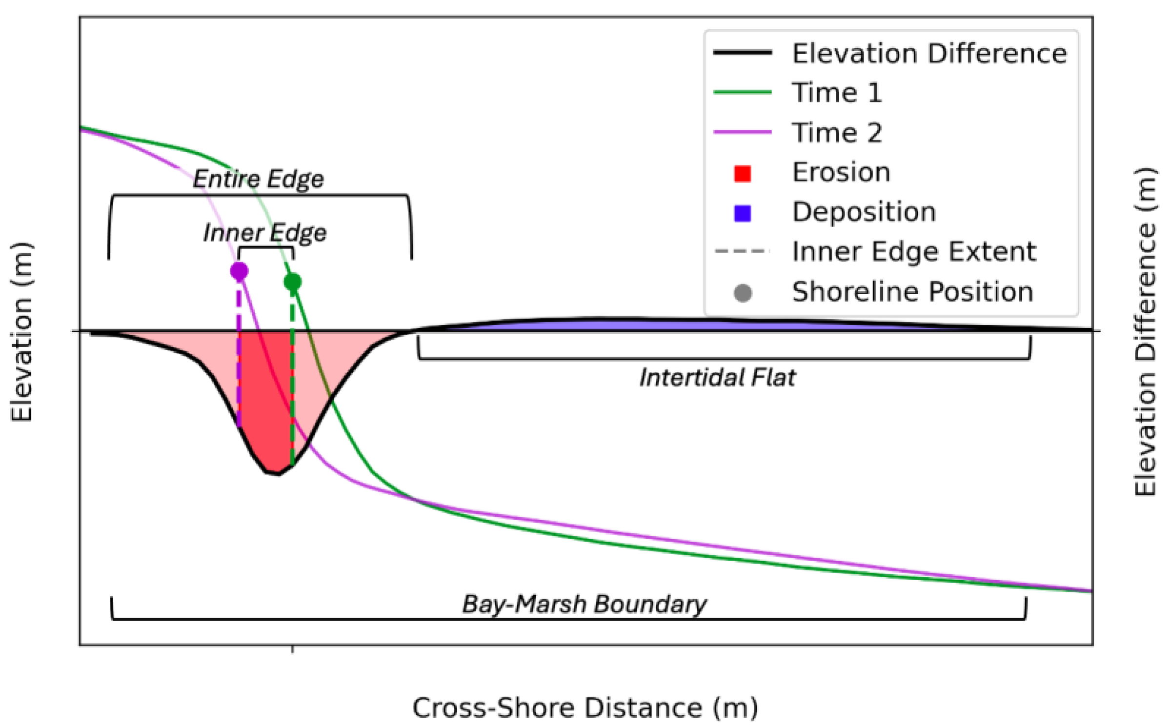
Figure 3.
Constructed GCPs installed onto (A) the marsh platform and (B) the intertidal flat.
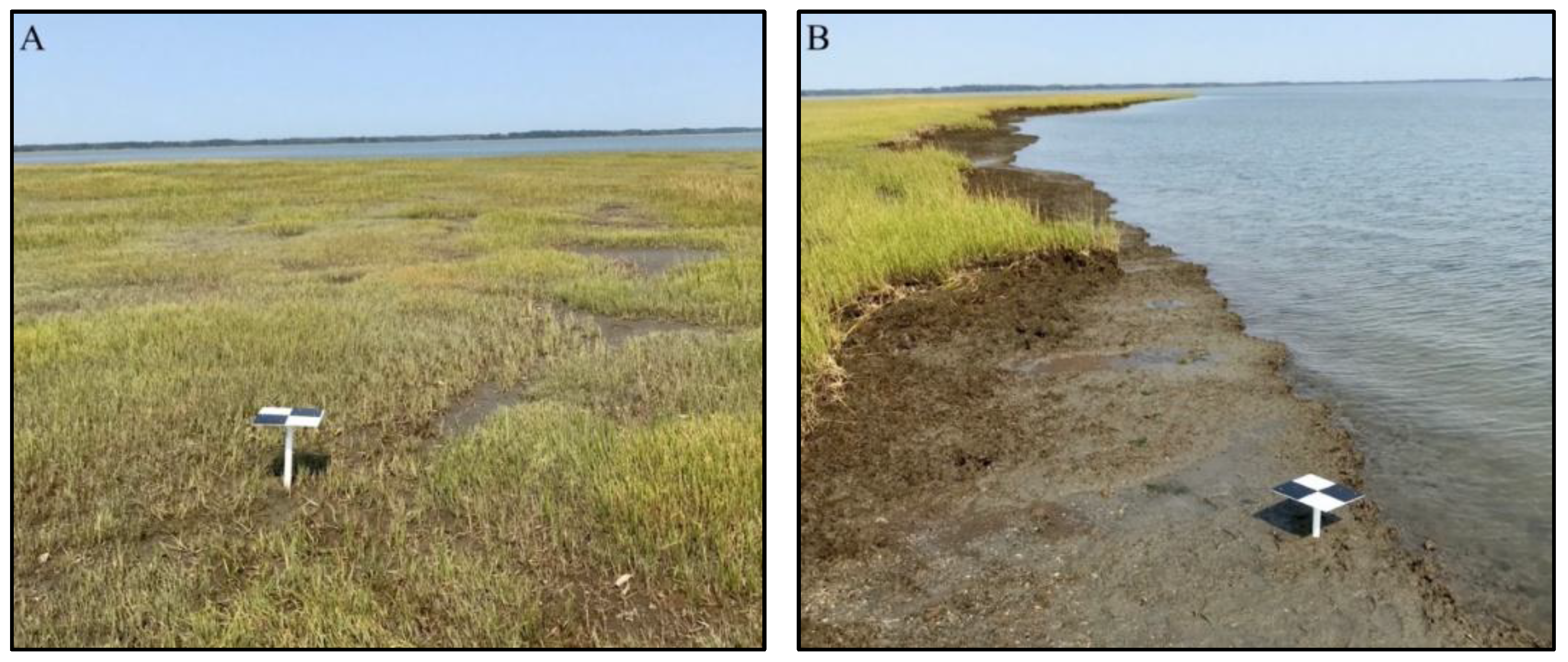
Figure 4.
Cross-sectional schematic of a retreating bay-marsh boundary at time 1 and time 2 with the colored dotted lines representing the location of the marsh shorelines. Black dots, A-D, represent the elevation measurements used to estimate marsh edge height and approximate volumetric change.
Figure 4.
Cross-sectional schematic of a retreating bay-marsh boundary at time 1 and time 2 with the colored dotted lines representing the location of the marsh shorelines. Black dots, A-D, represent the elevation measurements used to estimate marsh edge height and approximate volumetric change.
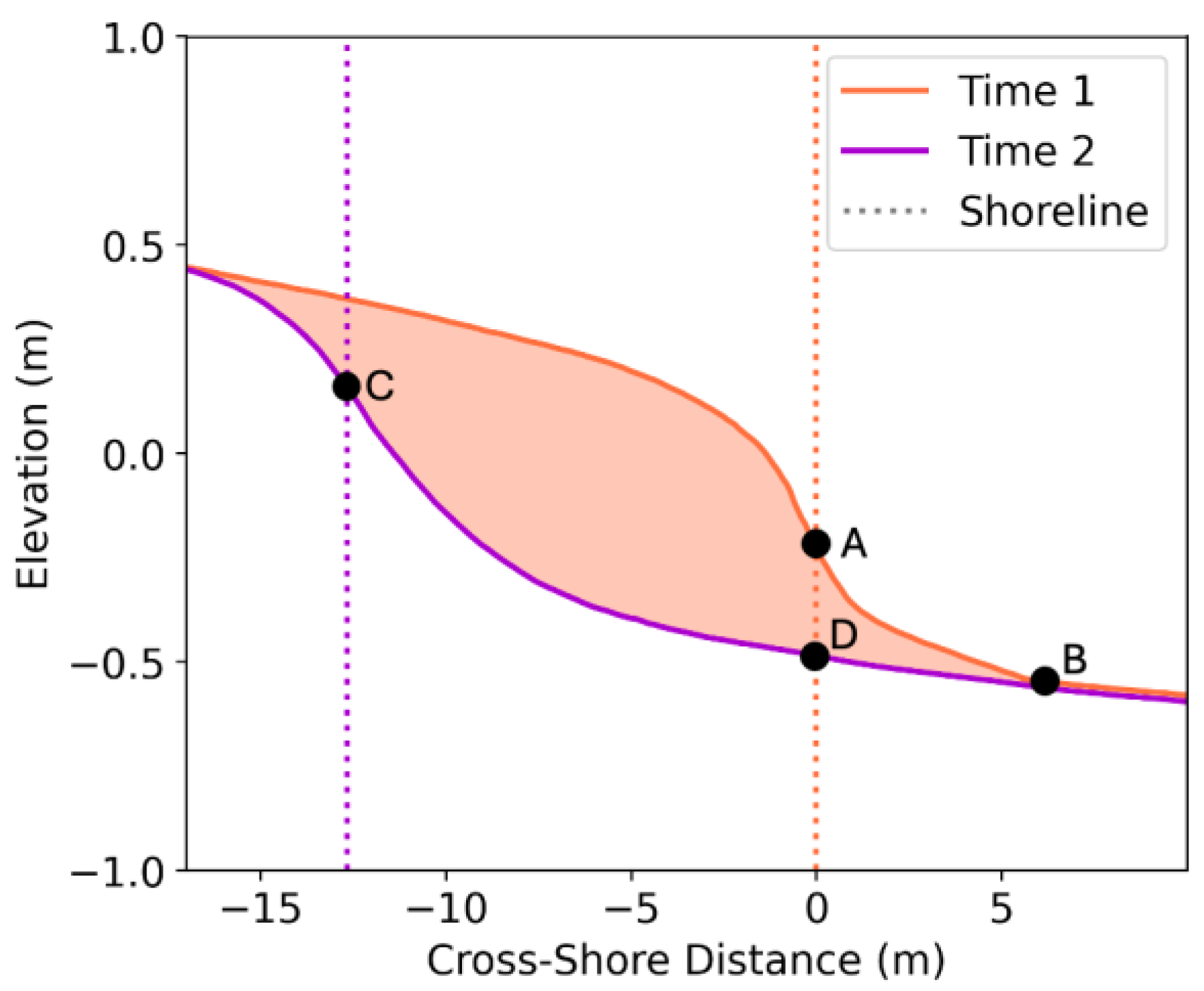
Figure 5.
Scatter plot comparing estimated to true elevations from 2023 where solid/dashed black lines represent the best-fit line for SfM/echosounder validation respectively and the grey line represents a 1-1 relationship. SfM data (estimate) is compared to RTK data (true) and colored based on feature. Echosounder data (estimate) is compared to SfM data (true) in red and collected solely in the intertidal flat.
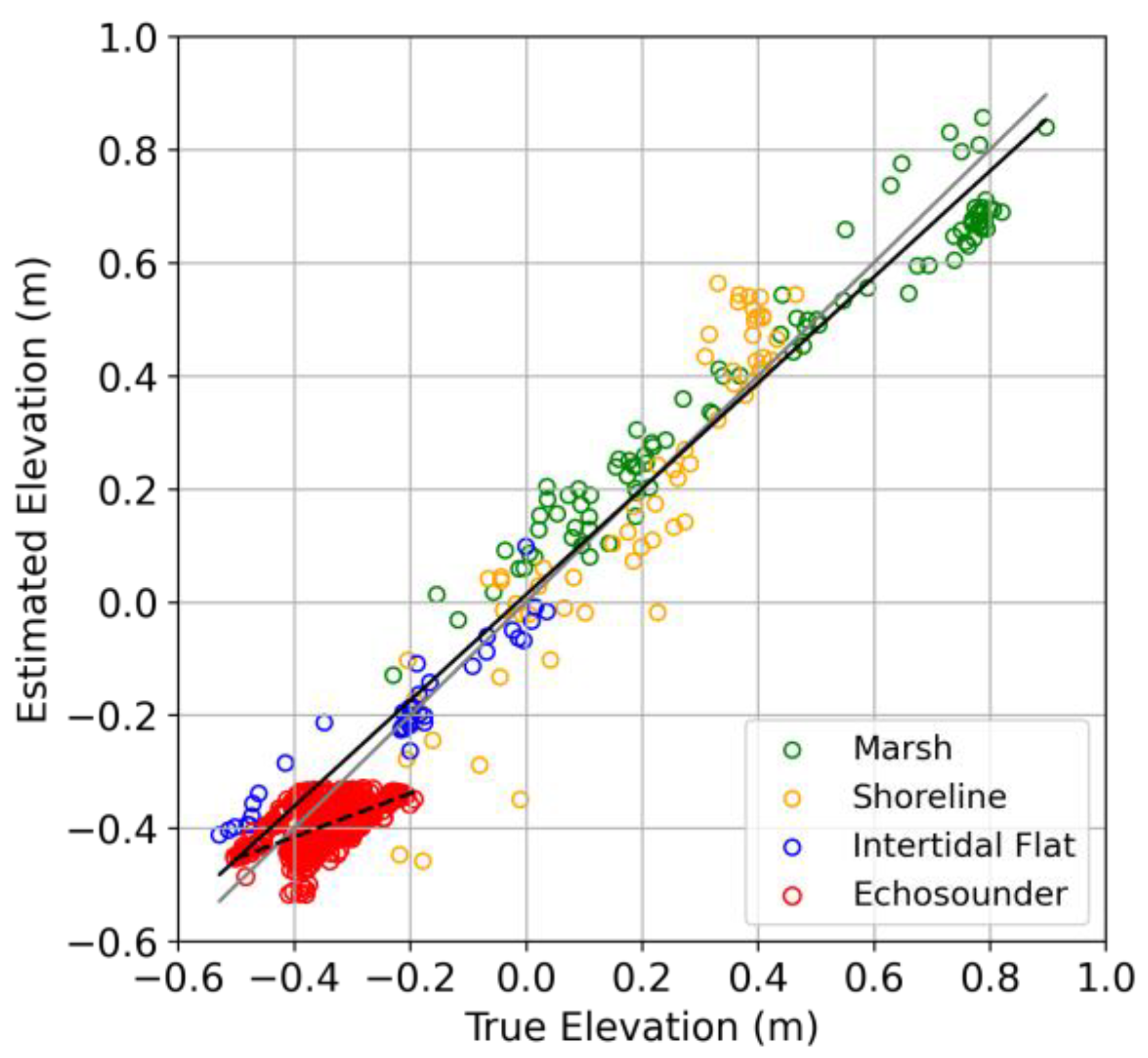
Figure 6.
(A) Orthomosaic of SP from 2023. (B) Topobathymetric DEM with tidal datums (MLLW, MSL, and MHHW) plotted as white lines. The horizontal black lines denote the transition from the northwest region (NW), the oyster reef region (Reef), and southeast region (SE). (C) Closeup of the DEM and (D) orthomosaic. (E) Difference maps comparing 2022 to 2023 and (F) 2015 to 2023, with the respective shorelines plotted.
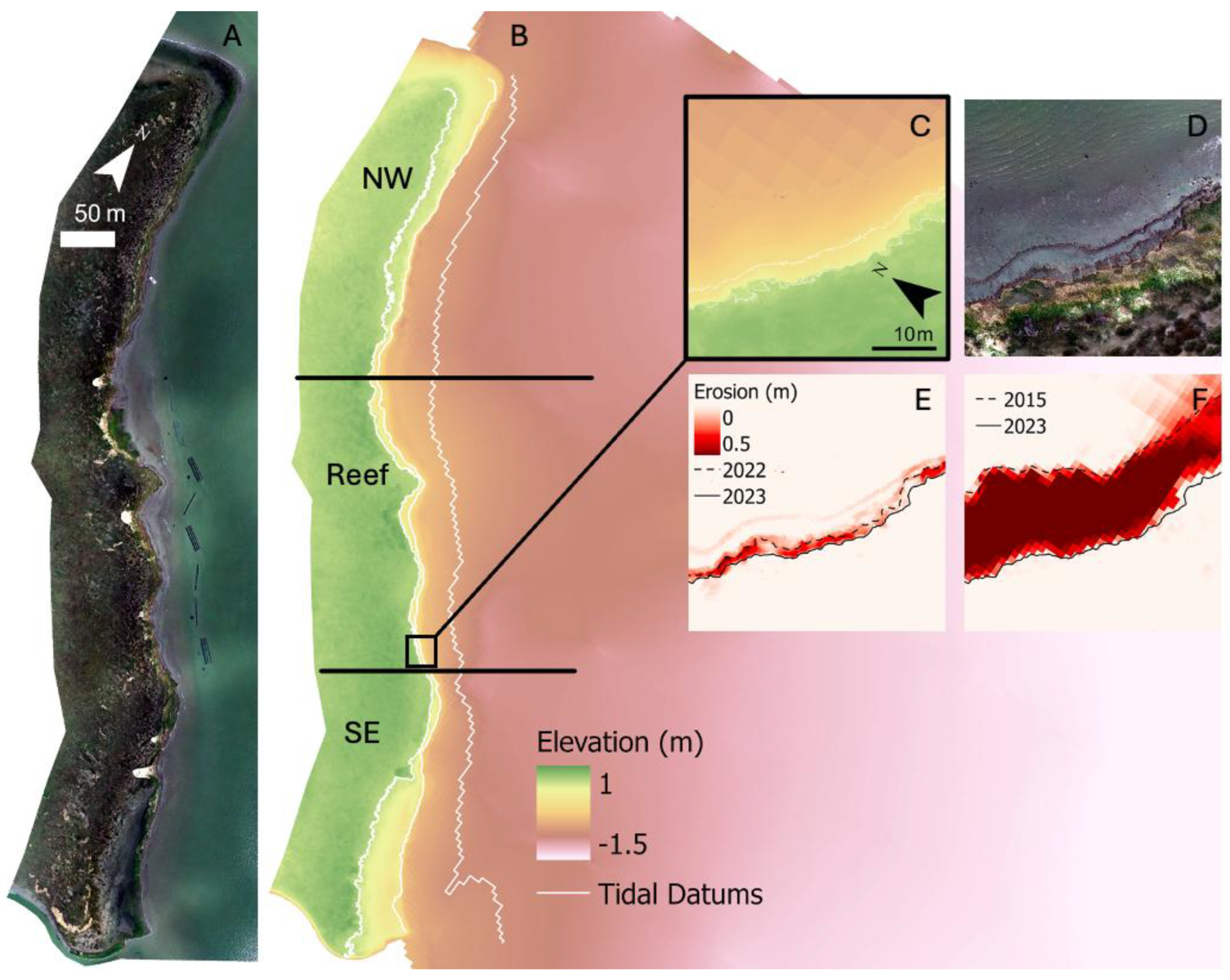
Figure 7.
Elevation profiles showing the cross-sectional morphology of the bay-marsh boundary across the entire study site. The solid lines represent the mean elevation of all transects within 1 m horizontal bins. Shading is the standard deviation, and error bars represent . The x-axis is zeroed at the location of the 2015 shoreline.
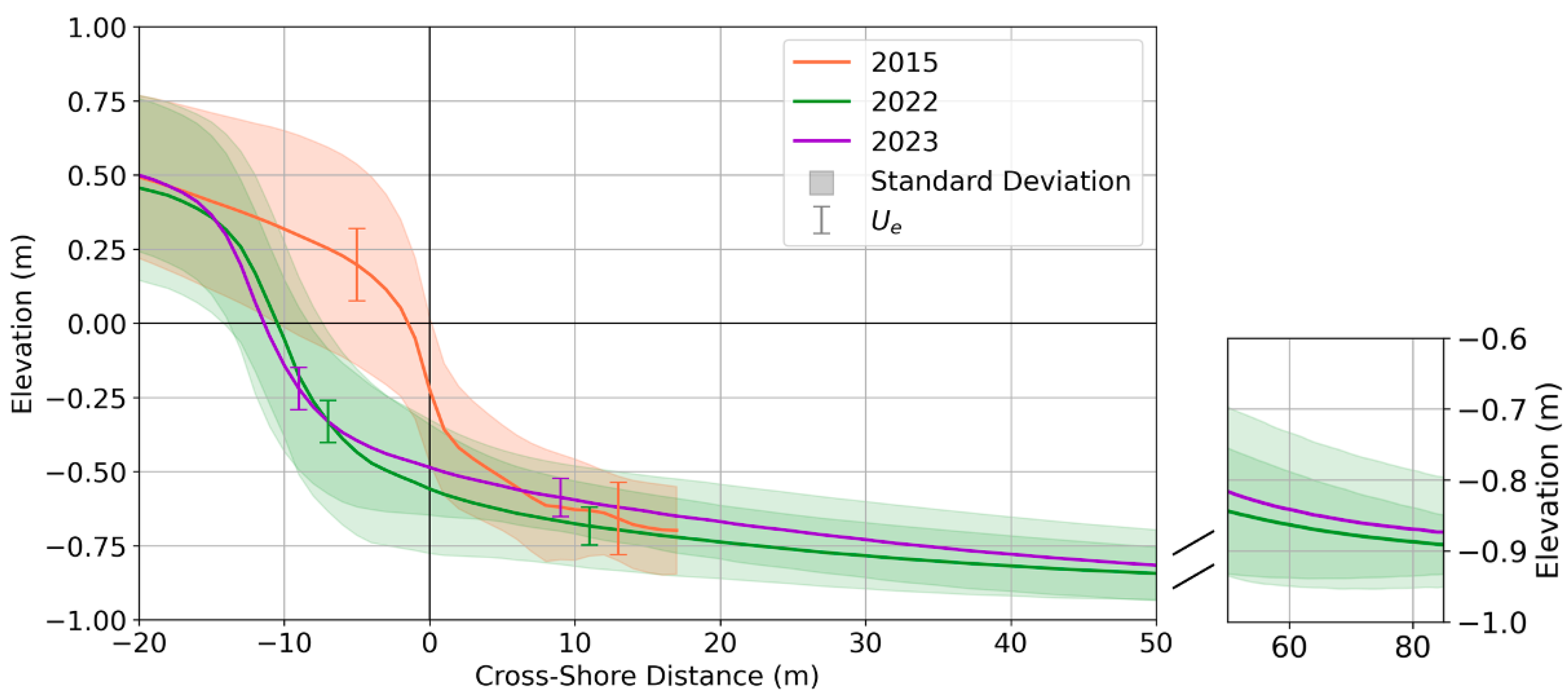
Figure 8.
(Left) Lateral change rates at the 8-year and annual timesteps separated by region where the dots represent the mean, the error bars represent uncertainty , and the boxes are the interquartile range. (Right) Map of lateral change rates zoomed in to the NW region of SP with the 8-year timestep plotted just offshore of the annual timestep.
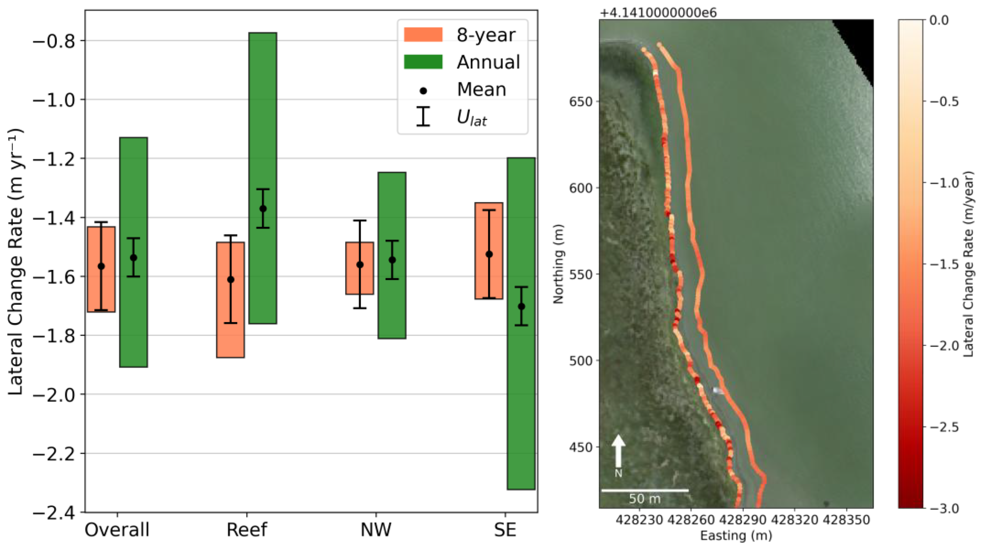
Figure 9.
Elevation difference profiles at the 8-year and annual timesteps. The solid colored lines represent the mean elevation profile for a given year as in Figure 7. Solid black lines are the elevation differences, with the standard deviation represented by the grey shading and the as error bars. The red shading represents erosion of the edge; darker red shading is the inner edge specifically; blue shading is deposition in the intertidal flat. The x-axis is zeroed at the location of the 2015 shoreline at the 8-year timestep and the 2022 shoreline at the annual timestep.
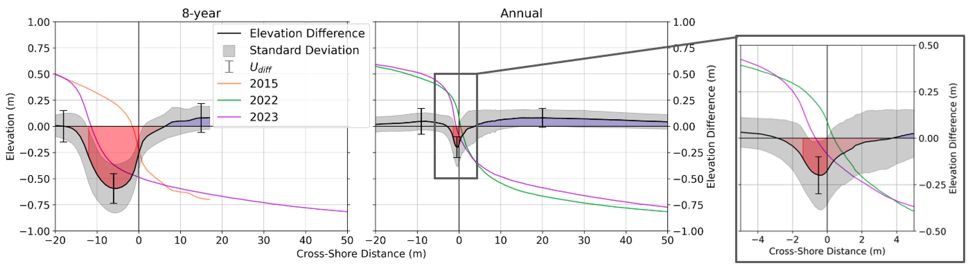
Figure 10.
Mean volumetric change rates as dots and as the error bars. Boxes represent the interquartile range. Separated by timestep and morphodynamic zone.
Figure 10.
Mean volumetric change rates as dots and as the error bars. Boxes represent the interquartile range. Separated by timestep and morphodynamic zone.
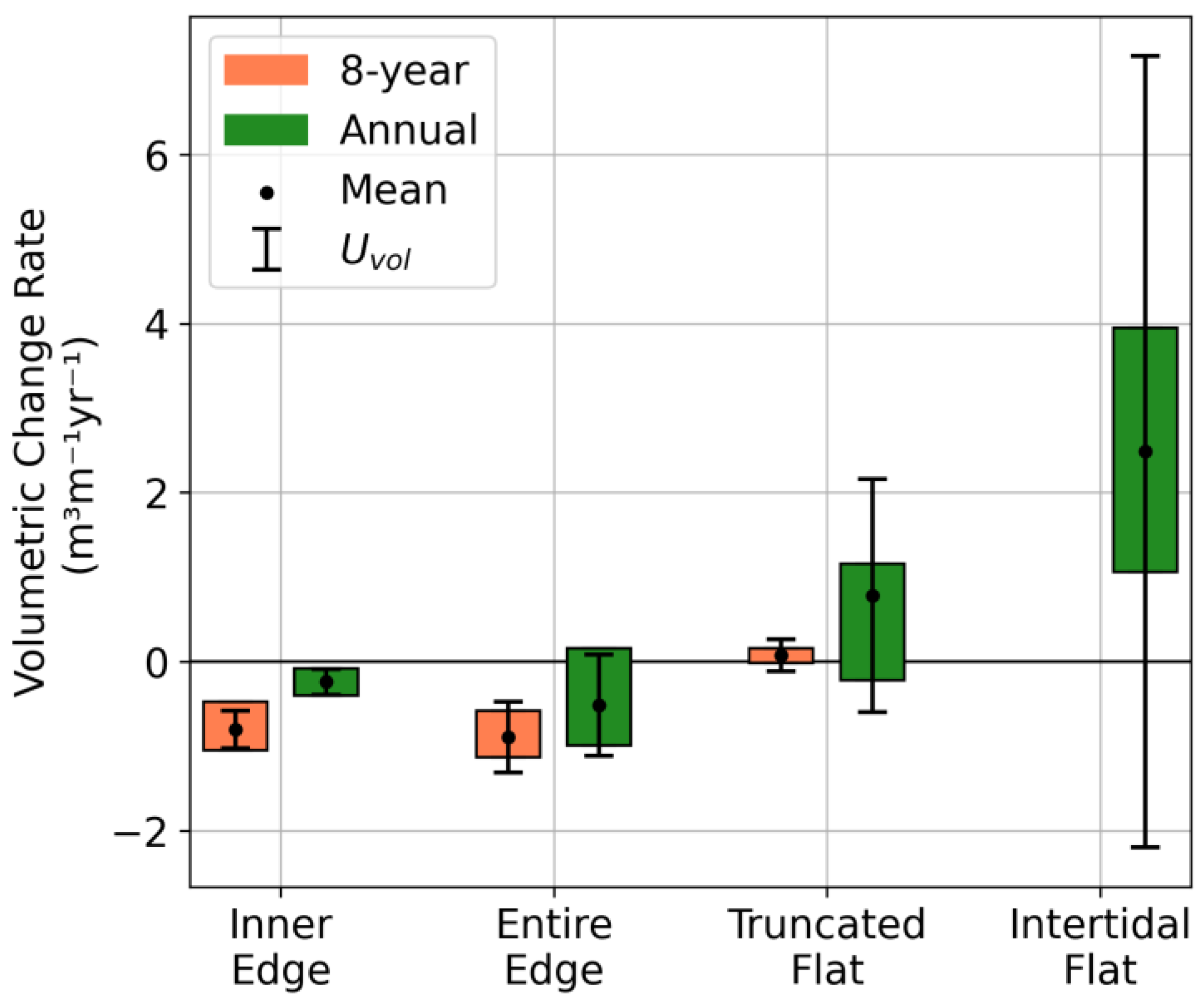
Figure 11.
Density plots of volumetric change rates of the marsh edge per alongshore distance for each transect, based on 2 approaches of estimating volumetric change rates with limited vertical data. The measured values of the inner edge are from the comprehensive analysis provided above.
Figure 11.
Density plots of volumetric change rates of the marsh edge per alongshore distance for each transect, based on 2 approaches of estimating volumetric change rates with limited vertical data. The measured values of the inner edge are from the comprehensive analysis provided above.
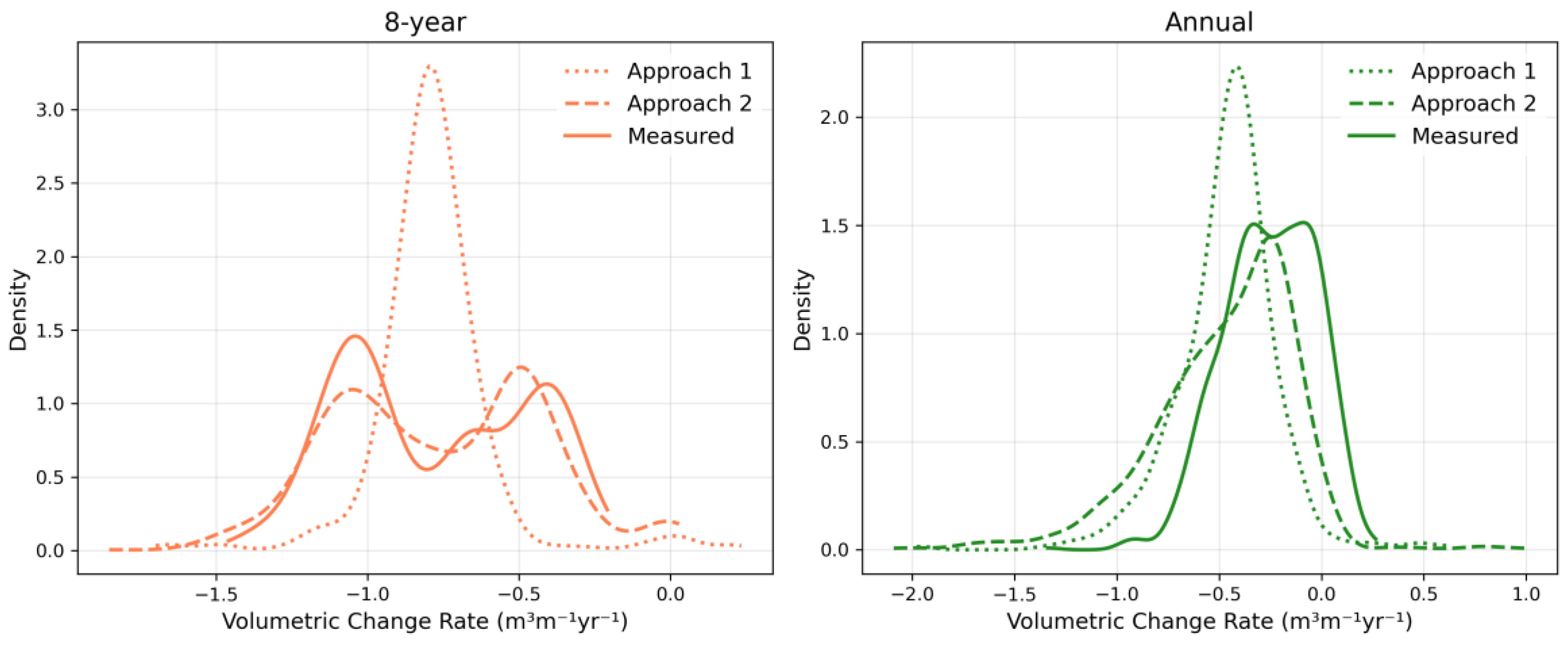
Figure 12.
Contours of the -0.5 m elevation for 2015 (before oyster reef installment) and 2022 (after oyster reef installment). The vertical black lines delineate the NW, Reef, and SE regions.
Figure 12.
Contours of the -0.5 m elevation for 2015 (before oyster reef installment) and 2022 (after oyster reef installment). The vertical black lines delineate the NW, Reef, and SE regions.
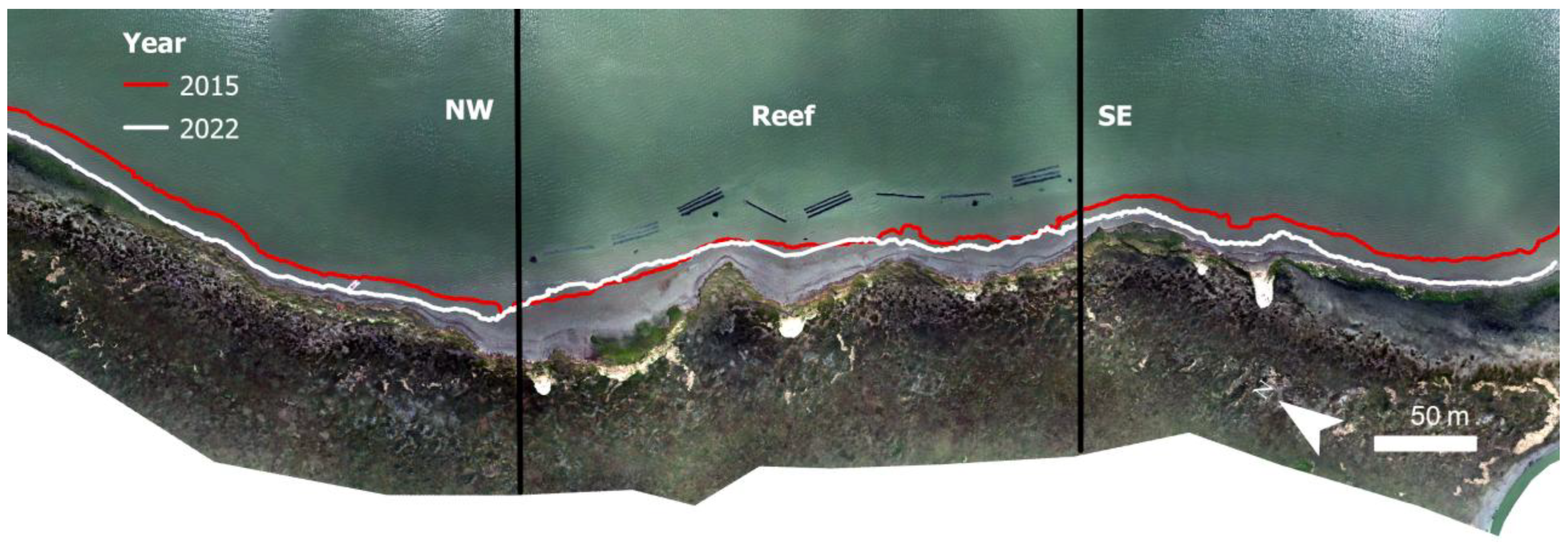

Table 1.
(m) for SfM data (estimate) compared to RTK data (true) in 2023 and separated based on feature. Echosounder data (estimate) is compared to SfM data (true).
Table 1.
(m) for SfM data (estimate) compared to RTK data (true) in 2023 and separated based on feature. Echosounder data (estimate) is compared to SfM data (true).
| Overall | Marsh | Shoreline | Intertidal Flat | Echosounder |
| 0.07 | 0.09 | 0.11 | 0.06 | 0.06 |
Table 2.
Lateral change rate means (m yr-1), uncertainty , and standard deviations (SD).
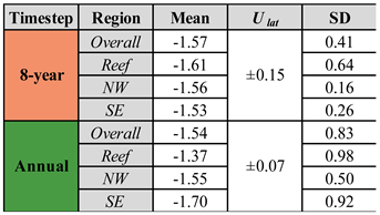
Table 3.
The mean and standard deviation of volumetric change rates per alongshore distance (m3 m-1 yr-1) and (m3 m-1 yr-1) for each morphodynamic zone and region for both the 8-year and annual timestep.
Table 3.
The mean and standard deviation of volumetric change rates per alongshore distance (m3 m-1 yr-1) and (m3 m-1 yr-1) for each morphodynamic zone and region for both the 8-year and annual timestep.
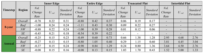
Table 4.
Mean and standard deviation of estimates of volumetric change rates (m3 m-1 yr-1) using limited vertical data compare to measured rates of the inner edge.
Table 4.
Mean and standard deviation of estimates of volumetric change rates (m3 m-1 yr-1) using limited vertical data compare to measured rates of the inner edge.
Disclaimer/Publisher’s Note: The statements, opinions and data contained in all publications are solely those of the individual author(s) and contributor(s) and not of MDPI and/or the editor(s). MDPI and/or the editor(s) disclaim responsibility for any injury to people or property resulting from any ideas, methods, instructions or products referred to in the content. |
© 2025 by the authors. Licensee MDPI, Basel, Switzerland. This article is an open access article distributed under the terms and conditions of the Creative Commons Attribution (CC BY) license (http://creativecommons.org/licenses/by/4.0/).
Copyright: This open access article is published under a Creative Commons CC BY 4.0 license, which permit the free download, distribution, and reuse, provided that the author and preprint are cited in any reuse.


