
Submitted:
10 April 2025
Posted:
10 April 2025
You are already at the latest version
Abstract
The Volume-of-Fluid (VOF) method is widely used for multiphase flow simulations, where the VOF function implicitly represents the interface through the volume fraction field. The height function (HF) method on a Cartesian mesh integrates the volume fractions of a column of cells across the interface. A stencil of three consecutive heights and centered finite differences computes the unit normal n and the curvature κ with second-order convergence with grid refinement. The interface line can cross more than one cell of the column and the value of the geometrical properties of the interface should be interpolated in the cut cells. The continuous height function is used to show that a constant approximation of the two geometrical properties across the column provides first-order convergence, while linear or quadratic interpolations provide second-order convergence. The numerical results agree with the theoretical development presented in this study.
Keywords:
interface reconstruction
; VOF/PLIC method
; height function method
; curvature
; two-phase flow
1. Introduction
Multiphase flows with moving interfaces separating immiscible fluids are present in many natural phenomena and industrial applications. These flows are often characterized by high density and viscosity ratios, a wide range of spatial scales and strong deformation of the interface due to surface tension that may produce complex topologies with interface merging or splitting. The surface tension force, located at the fluid-fluid interface, can be modelled by a force per unit volume, using the continuum surface force (CFS) model [1], , where is the surface tension coefficient and a surface distribution localized at the interface [2]. The accuracy of the CSF model requires a precise calculation of the interface geometry, in particular of the local values of the interface unit normal and of its curvature , in the computational cells that are cut by the interface. Several methods have been proposed to follow the time evolution of a moving interface, examples include, among others, the Volume of Fluid (VOF) method [3], the Level Set (LS) method [4] and the Front-Tracking (FT) method [5].
The VOF method considers the fraction of volume of any computational cell to represent implicitly the interface between two immiscible fluids
where is the volume of the cell and the phase indicator function with value 1 inside the reference phase and 0 in the secondary phase.
The advection of the volume fraction field depends on the local fluid velocity and satisfies the following advection equation
A geometrical, rather than algebraic, approach is required to solve Eq. (1) in order to minimize the numerical diffusion of the interface. To this aim, the interface should be reconstructed as a first step. The Piecewise Linear Interface Calculation (PLIC) approximates in two dimensions the interface line as a segment in each cut cell, , where the non homogeneous term is computed by enforcing area conservation [6]. Various schemes have been proposed to estimate the unit interface normal in a uniform Cartesian mesh, for example [7,8,9]. Mass-conservative advection schemes have been developed to compute phase fluxes across the cell boundary from the reconstructed interface in two dimensions (2D) [10] and three dimensions (3D) [11]. They can still produce very small mass errors due to finite machine precision, that should be removed during the numerical simulations.
In the height function (HF) method the heights are computed by summing across the interface the volume fractions of a column of cells of a Cartesian mesh. The height in a column is an approximation of the distance of the interface point on the column midline from a reference coordinate line, as shown in Figure 1a. Three consecutive heights along the same coordinate direction are required to compute the unit normal and the curvature with centered finite differences. The Standard Height Function (SHF) method uses a fixed stencil to calculate the three heights, while the Generalized Height Function (GHF) method uses an adaptive stencil to compute them [12]. The second approach is more precise at low resolution or in the presence of complex topologies that are characterized by interface breakup or coalescence. The HF method has also been extended to non-uniform Cartesian meshes [13], to adaptively refined meshes [12] and to unstructured meshes [14].
The HF method fails to provide adequate estimates of the interface geometry when the surface is not well resolved in the computational grid, in other terms, when the local radius of curvature is of the order of the grid spacing. A few hybrid methods have been developed to overcome this issue. At high grid resolutions, the unit normal and the curvature of the interface are computed with second-order convergence with the HF method. At lower grid resolutions the hybrid method should switch automatically to another more robust method with coarse meshes. The volume fraction field C can be convoluted with a smoothing kernel to obtain a more regular function (CV) [15]. Another possibility is the reconstructed distance function (RDF), which can be computed from the VOF function and the piecewise linear approximation of the interface [15], in a way similar to the coupled VOF-Level Set (CLSVOF) method [16]. The CV and the RDF functions can then be numerically differentiated to compute the curvature. Least-squared (LS) methods have also been proposed by fitting a parabola/paraboloid to the volume fractions of a block of cells [17] or to a set of interfacial points [12]. Other methods to compute the mean curvature include volumetric fitting methods [18].
More recently, a machine-learning approach has been used to estimate interface properties, directly from the volume fractions of a fixed block of cells [19,20,21], or even from the HF distribution [22]. The curvature estimate with this approach has not been shown to converge with mesh refinement, still it can be used at the lowest grid resolutions as a part of a hybrid method.
In some articles, the HF method is observed to have first-order convergence with grid refinement [20,21], while theoretical results indicate second-order convergence with mesh refinement. In this study, we investigate the reasons for this unexpected behavior and discuss a possible way to remove this inconsistency. Section 2 introduces the continuous height function of [23] and three different polynomial approximations of the interface line, of its unit normal and of the curvature in a column of cells cut by the interface. Section 3 considers an interface line described by a set of differentiable parametric equations and characterized by a variation of the curvature both in magnitude and sign. Second-order convergence with mesh refinement is recovered when the interface line is drawn in a uniform Cartesian grid at the points where the heights are located, but data interpolation provides a different order of convergence according to the polynomial approximation under consideration. Finally, our conclusions are drawn in Section 4.
2. Interface Line Approximation with the Height Function
2.1. The Continuous Height Function
Following the derivation of [23], we consider an interface line that locally can be espressed in the explicit form , when . The inverse form , should be considered when . We assume that is continuous with its derivatives, with the notation . The continuous height function is then defined as
is by definition the mean value of in the given interval of integration of length h. Similarly, the mean value of in the two adjacent intervals can be denoted as and . With these three consecutive values of the height function, it is possible to approximate with centered finite differences the value of the first and second derivatives and of the curvature of the function at point x
The first derivative represents the slope of the tangent line that determines uniquely the direction of the unit normal . With an expansion in the Taylor series with the small parameter h, it is straightforward to show that [23]
where and . The approximation of the function and of its derivatives and curvature with the height function H and centered finite differences is therefore second-order accurate with the grid spacing h. However, it should be noted that this statement is correct only at the abscissa x where the height point is located.
For the situation depicted in Figure 1a, the interface section inside the central column does not cross a horizontal grid line and the height , where the interface geometrical properties are evaluated, is centered with respect to that section. On the other hand, in Figure 1b the same interface line crosses a horizontal grid line in the central column. A centered scheme would require the computation of the geometrical properties at midpoints and , after the calculation of the position of the interface intersection with the grid line.
For the normal calculation, this issue was first raised in [24], where the numerical second derivative, given by the second of Eqs. (3), was used to approximate the variation of the unit normal across the column, and the abscissa of midpoints and was computed with an expression involving the volume fraction C of the two consecutive cut cells. For the curvature calculation, a quadratic interpolation, that was demonstrated to be second-order accurate, was proposed in [23], but numerical results were not provided.
Here, we consider three consecutive values of a geometrical property, for example the height function values , and of Figure 1a, to interpolate the data inside the central column. We compute the three coefficients
and consider the three polynomials , and , of order 0, 1 and 2, respectively
Let be the abscissa of the midpoint of the central column, then at any point x of the central column, with and , we find
The constant approximation is first-order accurate in the central cell, while the linear and quadratic interpolations, and , are both second-order accurate. These results are a direct consequence of the fact that the three height function values , and are second-order accurate.
In place of the height function values, we can consider three consecutive values of the first derivative and of the curvature, both of them defined in Eqs. (3), to recompute the coefficients a, b, and c of the polynomial approximations. For the first derivative, we find
and for the curvature
where . For both geometrical properties, we find again that the constant approximation is first-order accurate, while the linear and quadratic approximations are second-order accurate.
2.2. The Discrete Height Function
In a computational domain in two dimensions partitioned with square cells of side h, the volume fraction field C is initialized with the new version of the Vofi library [25], which requires a user-defined function . The interface is described by the implicit equation , points inside the reference phase satisfy , while in the secondary phase. The library computes the interface intersections with the grid lines and in each cut cell performs, where it is required, a 1D Gauss-Legendre integration with a variable number of nodes. The new version optimizes the algorithms described in [26], while introducing a few new features as well.
A grid cell cut by the interface will have , then the discrete height H can be calculated with a one-dimensional (1D) stencil by adding the C data columnwise, along the y direction, or rowwise, along the x direction. Let us consider only the vertical direction, where the interface line can be locally written in the explicit form , then
In the standard height function method (SHF) a fixed value of n is used, then the 1D stencil will have 5 cells for and 7 cells for . The height point H is centered in the i-th column, but it is not necessarily inside the cell . Furthermore, it is not guaranteed that the interface line crosses the entire column within the stencil, or there can be more than one interface section in the given stencil. This second situation may happen in the case of complex topologies, such as droplet merging or filament breakup.
The generalized height function method (GHF) considers an adaptive 1D stencil [12], centered at the mixed cell and with a maximum length of cells. The algorithm is dynamical, and the summation in (13) stops as soon as a full cell, , and an empty one, , are found on opposite sides of the stencil.
We usually consider a stencil with cells, then the height in the first two cases of Figure 2 is correctly computed, but not in Figure 2c as the stencil is not wide enough. However, in Figure 2c, the height can be computed along the x coordinate direction. In Figure 2d, there is an empty cell between the two interface sections, and the GHF method is capable of computing the two local heights; this is not the case for the SHF method. If the two sections approach each other even more and the empty cell disappears, both methods fail to provide an adequate height function value.
The height H is stored as an offset from the cell center together with a positive integer flag to indicate if the height is measured from the top or the bottom of the cell. Therefore, when we collect the heights to compute the interface geometrical properties, we need to normalize their value to a common base of the central column before computing the numerical derivatives. In the mixed cells with no height, the integer flag is set to a negative value to indicate that an interpolation of the local geometrical data is required in that cell.
At small grid resolutions, it is not always possible to collect three consecutive values of the height function that have been computed along the same coordinate direction. In that case, we can combine discrete heights computed columnwise and rowwise. This part of the algorithm has been discussed in [23]. In this study, we investigate only the asymptotic behavior of the height function method. In the present implementation of the algorithm, a first sweep across the computational domain is required to compute the discrete heights with Eq. (13), then a second sweep is performed to calculate numerically the interface geometrical properties with Eqs. (3). Finally, with a third sweep, these data are interpolated where necessary with the polynomials of Eqs. (11) and (12), after the evaluation of the interface intersections with the grid lines with Eqs. (9).
3. Numerical Results
3.1. Analytical Test Case
To recover numerically the theoretical results of the previous section, we consider an interface line that requires the use of the height function along both coordinate directions, that is characterized by a variation of the curvature value both in magnitude and sign and where the curvature can also be computed analytically. To this aim, we consider the 4-petaled star, that was introduced in [21], with parametric equations
where is the radius of the base circle, the amplitude of the oscillation and the number of oscillations (or petals). The interface line is drawn in Figure 3a. However, because of the symmetry of the figure, we consider only the portion of the line in the top-right quadrant where the angle varies in the range . The straight line is another axis of symmetry, as also pointed out by the numerical results. We subdivide the square domain of side with square cells of side , where is the grid resolution. The coarsest resolution is , i is the resolution level, . and . A small portion of the computational grid at the lowest resolution is also shown in Figure 3a.
If the height function is numerically computed with Eq. (13) along the vertical direction y, we are approximating with the first one of Eqs. (3) the first derivative at position x with centered finite differences. Given the parametric representation of Eqs. (14) and (15) of the interface line, and with the notation and , we compute analytically the required derivatives as
and then the curvature as
These derivatives are computed at the abscissa of the midpoint of the different columns, with . In the top-right quadrant of Figure 3a, Eq. (14) is strictly monotonic and can be numerically inverted to express the angle as a function of x.
In a similar manner we can compute analytically the derivatives of the inverse function at the ordinate and plot them as a function of the angle after the inversion of Eq. (15). Therefore, we can plot the first derivatives and as a function of the angle on the same figure, as shown in Figure 3b. The sections represented with solid lines are those where the first derivative of and of are smaller than one in absolute value. In the figure we observe three consecutive switches from one representation of the derivative to the other one. In Figure 3c we plot the second derivative and in Figure 3d the curvature, which is a geometrical property of the line that does not depend on the analytical representation.
3.2. Pointwise Convergence
The minimum radius of curvature , or the maximum curvature , is found at , where . In that point the absolute value of the first derivative is equal to one, and there is a switch in the representation of the first derivative. For these two reasons, the error of the numerical approximation of the curvature is expected to be maximum. In Figure 4a we consider three consecutive columns, the middle one centered at the abscissa , computed from Eq. (14). The value H of the three heights is calculated with the Vofi library and the numerical first derivative and curvature with Eqs. (3). The local error for a geometrical property q is defined as follows
where is the analytical value at and the numerical value at resolution level i. The thickness of the largest column is , corresponding to level , that of the most slender one is , of level .
We also consider a block of square cells of side h of the computational domain that was previously defined. The point of interest at is always contained in the central column of the block, as shown in Figure 4b for the first three grid resolutions.
The midpoint of the central column provides an approximation of the abscissa , and it coincides with the root approximation of given by the bisection method. The sequence of midpoints is then approaching the value with the linear convergence of the bisection algorithm. In this case, we can define two local errors
where is the numerical value of q at from the three heights in the block and is the analytical value at . The results for the first derivative and the curvature at are shown in Figure 5. A second-order convergence is observed for the three different local errors, even if the sequence converges only linearly to . The fluctuation in the values of and is due to the fact that the error is maximum at and that the point can get very close to at any grid spacing h and then moves away at the next refinement, as typical of the bisection method.
3.3. Convergence to the Interface Line
In Figure 3, we have plotted the interface line, its first and second derivatives, and the curvature as a function of the angle . Sections of the different lines are drawn as solid lines where the first derivative of the function or of the inverse function are smaller than or equal to 1 in absolute value. In these sections, we compute the error at the abscissa or ordinate , where the height function is defined, for any geometrical property q as
where is the numerical value computed from the height function field and the corresponding analytical value.
As we double the grid resolution from cells to , the number of heights along each coordinate direction also roughly doubles. To keep that number more or less constant in a plot, we divide that number by the factor , where i is the resolution level that was previously defined. Similarly, for a second-order convergence, the error of Eq. (20) should decrease by the factor 4 from one resolution level to the next one. Again, to keep that value more or less constant at each abscissa , or ordinate , we multiply it by the factor , . In Figure 6, we plot the error of the height function, of its first and second derivatives, and of the curvature as a function of the angle . In Figure 6a, the three switches from one representation of the interface line to the other are seen as cusps. The error is maximum at , as previously anticipated. In the other plots, the error is still continuous at , because of the symmetry of the interface line with respect to that axis, but not in the other two transitions. A few minima appear in the plots that are due to error cancellation for the corresponding values of the angle .
The error of the height function model for any geometrical property q can be evaluated by the norm defined as
and by the norm
where again is the numerical value from the height function field, the analytical value at the same position , or , and the total number of cells where the height is positioned, at resolution level i.
The results for the two error norms are presented in Figure 7 for the first derivative and curvature. A second-order convergence is observed for both norms and geometrical properties.
3.4. Data Interpolation
The numerical results obtained in the previous section are in agreement with the theoretical development of Section 2.1, namely that the discrete height function approximation, given by Eq. (13), and the numerical approximation of its geometrical properties, given by Eqs. (3), are second-order accurate at the points where the height H is positioned. The vertical heights of Figure 1a are along the midline of each column. However, if the interface section inside the column crosses a horizontal grid line, as shown in Figure 1b, the two subsections of the interface lie on different grid cells. The issue is now which value should be considered for the normal vector and for the local curvature.
In Figure 1a, a translation of the interface line parallel to itself along the vertical direction changes the value of the three heights H by the same amount and the position of the intersection point with the horizontal grid line in Figure 1b as well. However, the value of the first and second derivatives and the curvature does not change. Therefore, to simplify the derivation, in the columns, or rows, where the height function is located, we consider the subgrid spacing and the positions at , with , for a total of 8 points. At each refinement level i, we then have additional points and the same two error norms of Eqs. (21) and (22). The value is again the analytical value of the geometrical property q computed at the additional points. In contrast, the numerical value is now computed with one of the three polynomial interpolations of Eqs. (9). The coefficients a, b and c are calculated from three consecutive values of q, as illustrated in Eqs. (8).
Figure 8 and Figure 9 show the convergence of and error norms for the interpolation of the first derivative and of the curvature, respectively. These results agree with the theoretical ones of Eqs. (11) and (12). The constant approximation shows first-order convergence. This is by far the most commonly-used approximation in two-phase flow simulations with the one fluid formulation of the Navier-Stokes equations. The linear and quadratic interpolations compute the first derivative more accurately with second-order convergence. This interpolation should be used at any grid resolution only when the interface line intersects a horizontal grid line in a given vertical column, as shown in Figure 1b, but not for example in the two adjacent columns. For the interpolation, a few more computations need to be performed: geometrical data need to be collected from the two lateral columns (or rows), to approximate the intersection and the position of the two midpoints and , where the geometrical data need to be interpolated. On a local Cartesian coordinate system with the origin on the bottom-left corner, the abscissa of the two midpoints are and , respectively.
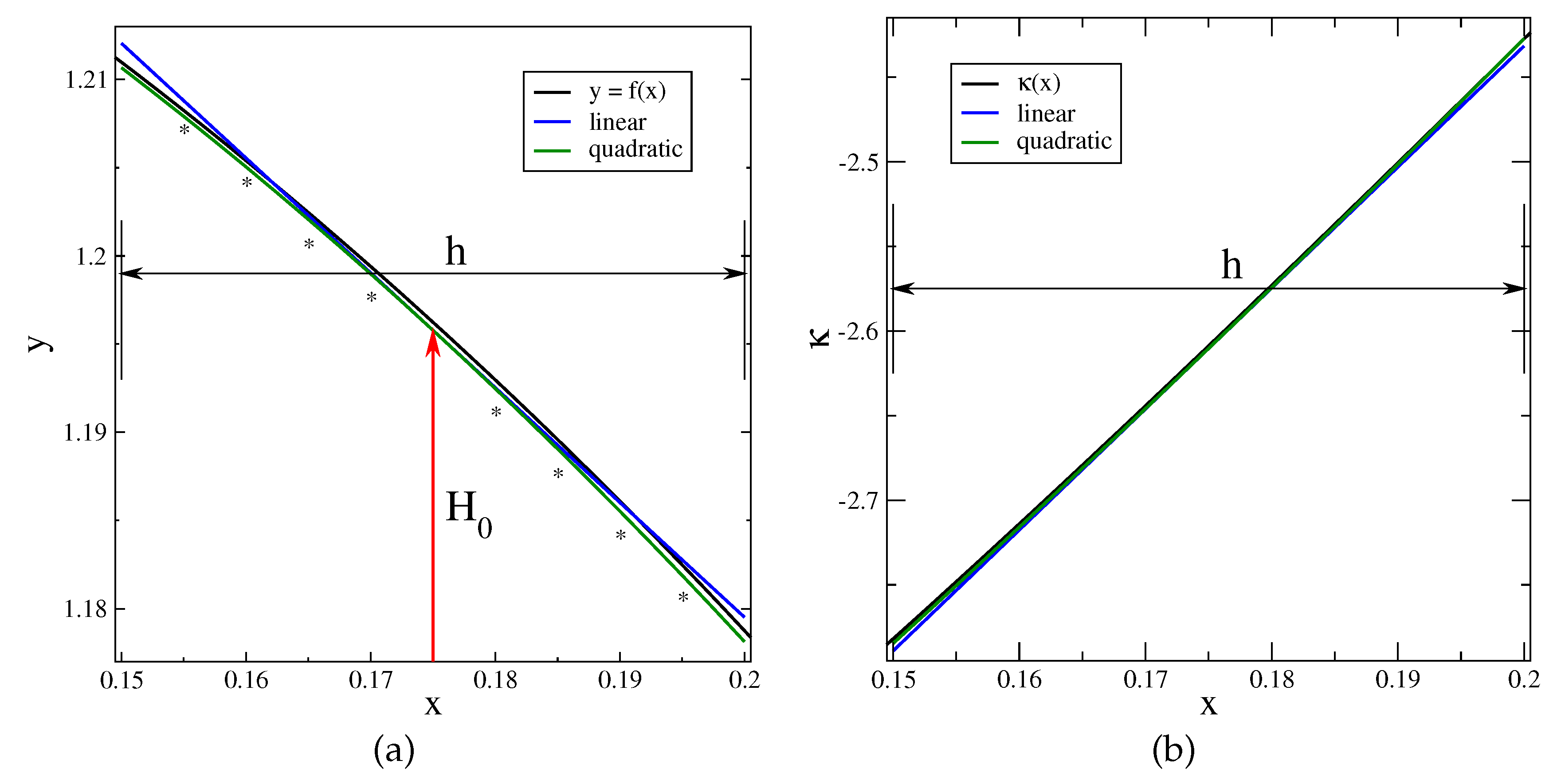
It is not surprising that the linear and quadratic interpolations show a similar behavior, since the geometrical properties q, that have been computed numerically, are only second-order accurate. Figure 10a shows the linear and quadratic approximations of the interface line calculated from three consecutive values of the height function H, in the vertical column with the abscissa x in the range , at the coarsest resolution, . The endpoint of the height H is always positioned in the convex region of the interface line, and the quadratic interpolation lies entirely in the same set. The central part of the linear approximation is also in the convex region. Still, it crosses the interface line, and the two endpoints of the linear interpolation are in the concave region. This implies that linear interpolation is closer to the interface line than the quadratic interpolation in a relevant fraction of the column size. The two interpolations are then comparable, and in any cut cell the “best” choice could be different according to the position of the intersection point and of the two midpoints and of Figure 1b. Figure 10b shows the linear and quadratic approximations of the interface curvature in the same column. The two interpolations are both in the convex region, and the quadratic one is somewhat closer to the analytical value.
4. Conclusions
In this study, we have considered the height function (HF) method for the representation of an interface line and the calculation of its geometrical properties. The HF method integrates the volume fraction (VOF) field along a column of grid cells of a Cartesian mesh and provides a smoother field to be differentiated with finite differences. We have chosen the generalized height function (GHF) approach, that considers an adaptive stencil for the VOF function integration, over the standard height function (SHF) approach, that considers a fixed stencil, because it computes more accurate heights, in particular in high curvature regions.
With the HF values from three consecutive columns of cells along the same coordinate direction and centered finite differences, the first and second derivatives of the interface line can be computed with second-order convergence with grid refinement. The unit normal and the curvature are then calculated along the column midline from these two derivatives.
The interface line can intersect more than one cell in a given column of a Cartesian mesh. When this happens, the interface geometrical properties have to be interpolated in the cut cells from the value in the column midline. We have considered three polynomials that correspond to constant, linear, and quadratic approximations of the interface line inside the column, respectively. The constant approximation is the most widely used and provides first-order convergence, the linear and quadratic approximations provide second-order convergence.
Finally, we have considered an interface line in a uniform Cartesian mesh. The interface is described by differentiable parametric equations and is characterized by a curvature changing both in magnitude and sign. The numerical results are in agreement with the theory we have presented.
Author Contributions
Conceptualization, A.C., S.M., J.P., R.S. and S.Z.; methodology, A.C., S.M., J.P., R.S. and S.Z.; software, A.C., S.M., J.P., R.S. and S.Z.; validation, A.C., S.M., J.P., R.S. and S.Z.; writing—original draft preparation, A.C., S.M., J.P., R.S. and S.Z.; writing—review and editing, A.C., S.M., J.P., R.S. and S.Z. All authors have read and agreed to the published version of the manuscript.
Funding
This research received no external funding.
Institutional Review Board Statement
Not applicable.
Informed Consent Statement
Not applicable.
Data Availability Statement
Dataset available on request from the authors.
Conflicts of Interest
The authors declare no conflicts of interest.
References
- Brackbill, J.U.; Kothe, D.B.; Zemach, C. A continuum method for modeling surface tension. J. Comput. Phys. 1992, 100, 335–354. [CrossRef]
- Tryggvason, G.; Scardovelli, R.; Zaleski, S. Direct Numerical Simulations of Gas-Liquid Multiphase Flows; Cambridge University Press, 2011.
- Hirt, C.W.; Nichols, B.D. Volume of Fluid (VOF) Method for the Dynamics of Free Boundaries. J. Comput. Phys. 1981, 39, 201–225. [CrossRef]
- Sussman, M.; Smereka, P.; Osher, S. A Level Set Approach for Computing Solutions to Incompressible Two–Phase Flow. J. Comput. Phys. 1994, 114, 146–159. [CrossRef]
- Tryggvason, G.; Bunner, B.; Esmaeeli, A.; Juric, D.; Al-Rawahi, N.; Tauber, W.; Han, J.; Nas, S.; Jan, Y.J. A Front–Tracking Method for the Computations of Multiphase Flow. J. Comput. Phys. 2001, 169, 708–759. [CrossRef]
- Scardovelli, R.; Zaleski, S. Analytical Relations Connecting Linear Interfaces and Volume Fractions in Rectangular Grids. J. Comput. Phys. 2000, 164, 228–237. [CrossRef]
- Youngs, D.L. Time–dependent multi–material flow with large fluid distortion. In Proceedings of the Numerical Methods for Fluid Dynamics; Morton, K.; Baines, M., Eds., New York, 1982; pp. 273–285.
- Pilliod, J.E.J.; Puckett, E.G. Second–order accurate volume–of–fluid algorithms for tracking material interfaces. J. Comput. Phys. 2004, 199, 465–502. [CrossRef]
- Aulisa, E.; Manservisi, S.; Scardovelli, R.; Zaleski, S. Interface reconstruction with least–squares fit and split advection in three–dimensional Cartesian geometry. J. Comput. Phys. 2007, 225, 2301–2319. [CrossRef]
- Aulisa, E.; Manservisi, S.; Scardovelli, R.; Zaleski, S. A geometrical area–preserving Volume–of–Fluid advection method. J. Comput. Phys. 2003, 192, 355–364. [CrossRef]
- Weymouth, G.D.; Yue, D.K.P. Conservative Volume–of–Fluid method for free–surface simulations on Cartesian–grids. J. Comput. Phys. 2010, 229, 2853–2865. [CrossRef]
- Popinet, S. An accurate adaptive solver for surface–tension–driven interfacial flows. J. Comput. Phys. 2009, 228, 5838–5866. [CrossRef]
- Francois, M.M.; Swartz, B.K. Interface curvature via volume fractions, heights, and mean values on nonuniform rectangular grids. J. Comput. Phys. 2010, 229, 527–540. [CrossRef]
- Ivey, C.B.; Moin, P. Accurate interface normal and curvature estimates on three–dimensional unstructured non–convex polyhedral meshes. J. Comput. Phys. 2015, 300, 365–386. [CrossRef]
- Cummins, S.J.; Francois, M.M.; Kothe, D.B. Estimating curvature from volume fractions. Computers and Structures 2005, 83, 425–434. [CrossRef]
- Sussman, M.; Puckett, E.G. A Coupled Level Set and Volume–of–Fluid Method for Computing 3D and Axisymmetric Incompressible Two–Phase Flows. J. Comput. Phys. 2000, 162, 301–337. [CrossRef]
- Renardy, Y.; Renardy, M. PROST: A Parabolic Reconstruction of Surface Tension for the Volume–of–Fluid Method. J. Comput. Phys. 2002, 183, 400–421. [CrossRef]
- Han, A.; Evrard, F.; Desjardins, O. Comparison of methods for curvature estimation from volume fractions. Int. J. Multiph. Flow 2024, 174, 104769. [CrossRef]
- Qi, Y.; Lu, J.; Scardovelli, R.; Zaleski, S.; Tryggvason, G. Computing curvature for volume of fluid methods using machine learning. J. Comput. Phys. 2019, 377, 155–161. [CrossRef]
- Patel, H.V.; Panda, A.; Kuipers, J.A.M.; Peters, E.A.J.F. Computing interface curvature from volume fractions: a machine learning approach. Comput. & Fluids 2019, 193, 104263.
- Önder, A.; Liu, P.L.F. Deep learning of interfacial curvature: A symmetry-preserving approach for the volume of fluid method. J. Comput. Phys. 2023, 485, 112110. [CrossRef]
- Cervone, A.; Manservisi, S.; Scardovelli, R.; Sirotti, L. Computing Interface Curvature from Height Functions Using Machine Learning with a Symmetry–Preserving Approach for Two–Phase Simulations. Energies 2024, 17, 3674. [CrossRef]
- Bornia, G.; Cervone, A.; Manservisi, S.; Scardovelli, R.; Zaleski, S. On the properties and limitations of the height function method in two–dimensional Cartesian geometry. J. Comput. Phys. 2011, 230, 851–862. [CrossRef]
- Ferdowsi, P.; Bussmann, M. Second–order accurate normals from height functions. J. Comput. Phys. 2008, 227, 9293–9302. [CrossRef]
- Chierici, A.; Chirco, L.; Chenadec, V.L.; Scardovelli, R.; Yecko, P.; Zaleski, S. An optimized VOFI library to initialize the volume fraction field. Comput. Phys. Commun. 2022, 281, 108506. [CrossRef]
- Bnà, S.; Manservisi, S.; Scardovelli, R.; Yecko, P.; Zaleski, S. Numerical integration of implicit functions for the initialization of the VOF function. Comput Fluids 2015, 113, 42–52. [CrossRef]
Figure 1.
(a) Three consecutive heights H are required to compute the interface unit normal and the curvature with centered finite differences at the midpoint x of the central column; (b) the interface section inside the central column crosses two consecutive grid cells, and the interface geometrical properties computed at point x should be interpolated at points and .
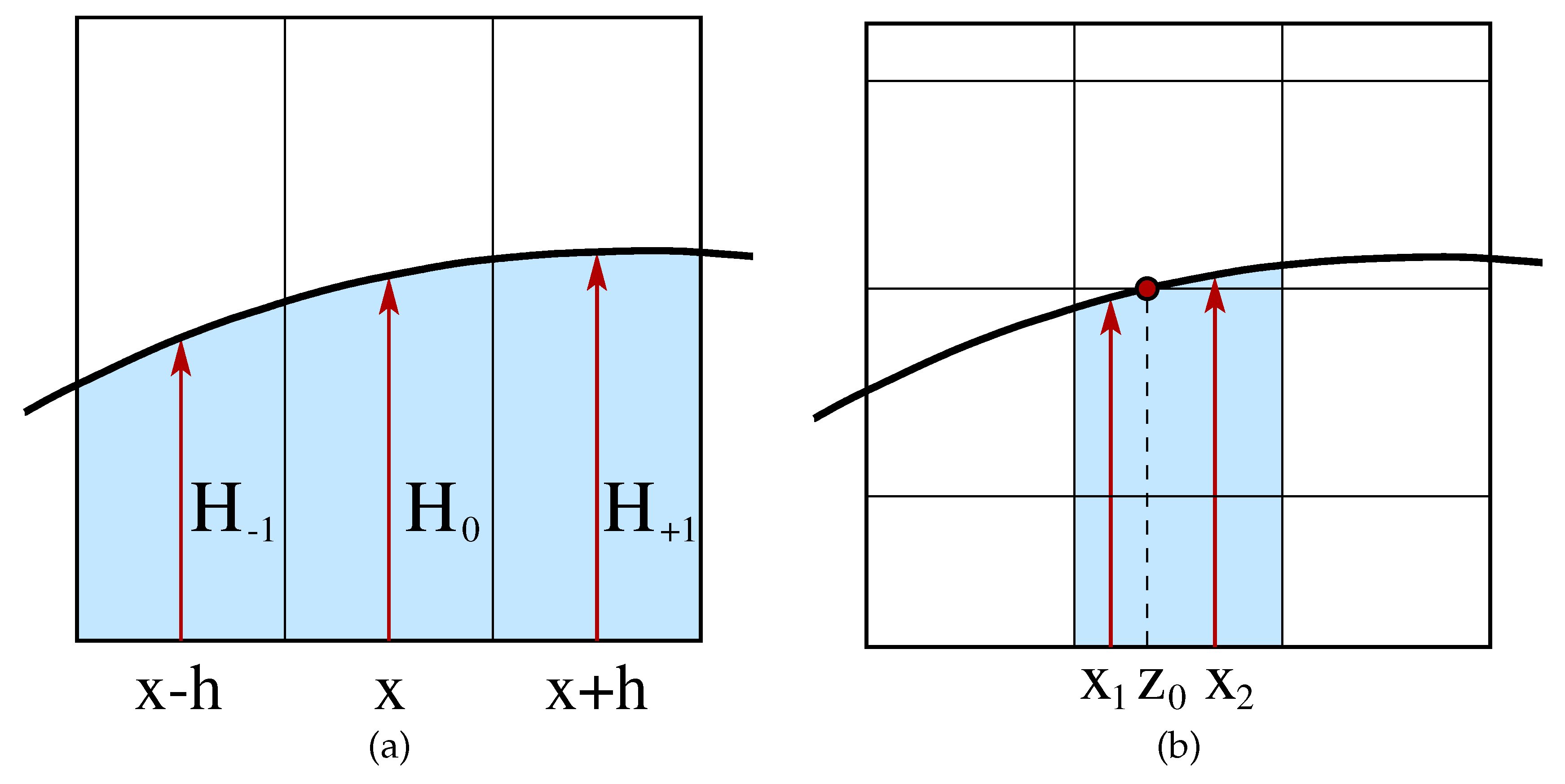
Figure 2.
Generalized height function (GHF) and a stencil with cells: (a) only three cells are required to compute the height; (b) the entire stencil is necessary; (c) the stencil is not wide enough, since the top cell is not empty; (d) both local heights can be computed.
Figure 2.
Generalized height function (GHF) and a stencil with cells: (a) only three cells are required to compute the height; (b) the entire stencil is necessary; (c) the stencil is not wide enough, since the top cell is not empty; (d) both local heights can be computed.
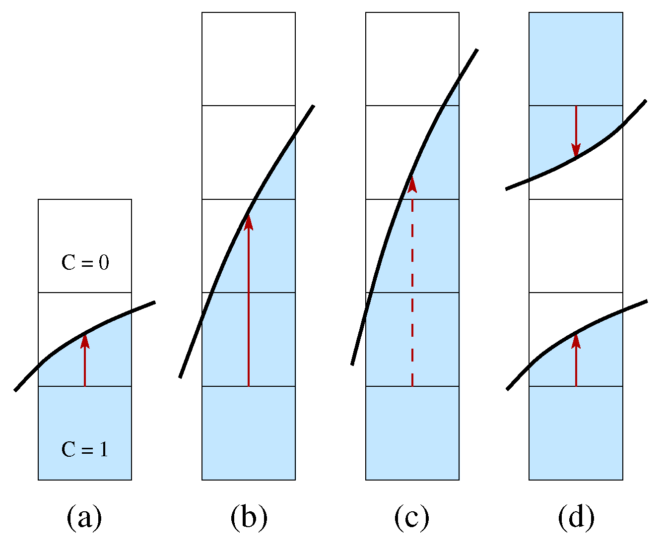
Figure 3.
(a) Base circle (green line) and 4-petaled star (indigo line), the top-right sector is the computational domain containing a quarter of the star (thick black line); (b) first derivative, (c) second derivative and (d) curvature as a function of the angle , computed from (red lines) and (blue lines); the sections shown as solid lines are those that are numerically approximated.
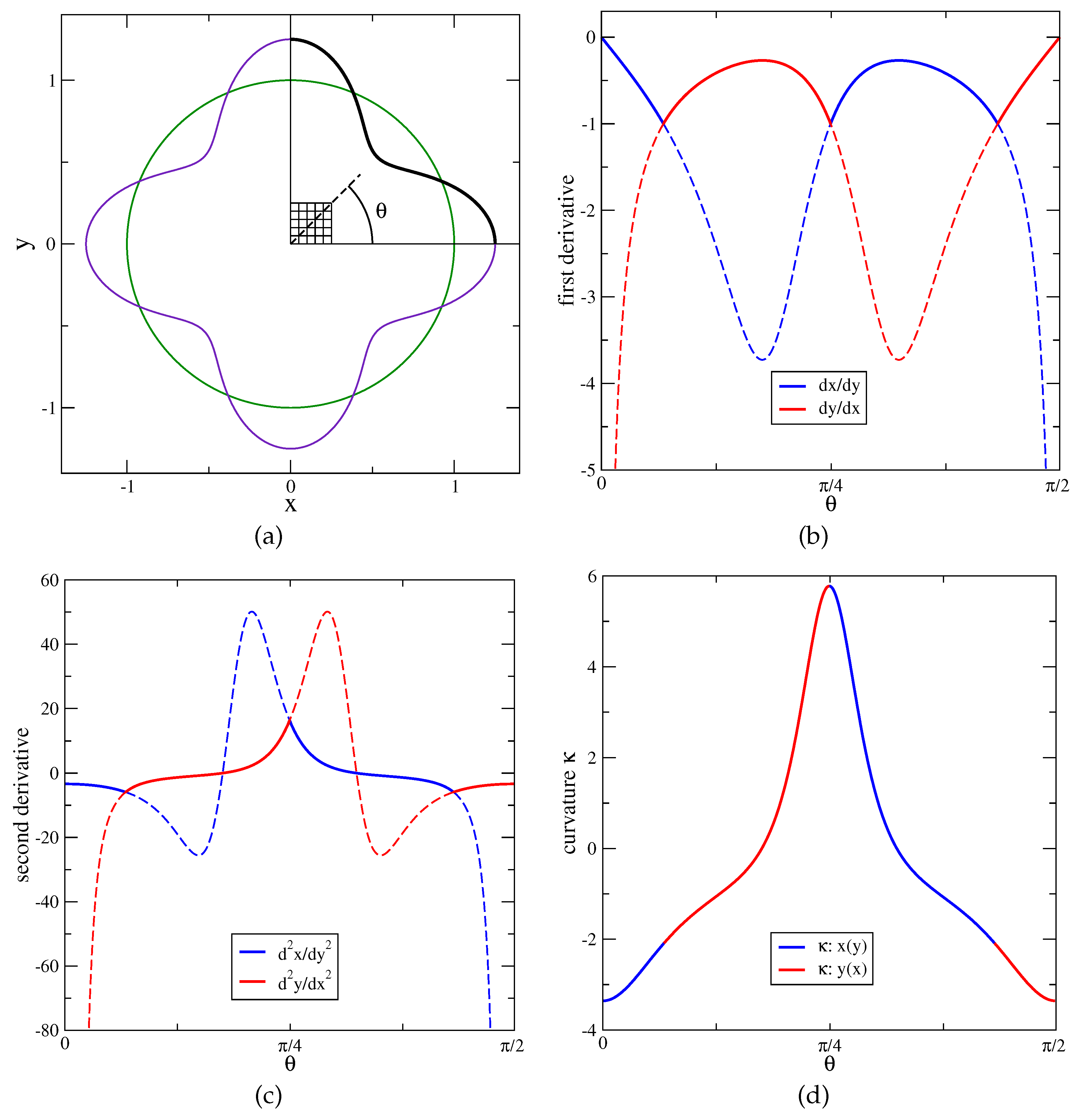
Figure 4.
Geometry to compute heights (red segments) near the point at (green point) of the interface (blue line). (a) Three consecutive columns with the largest spacing, , the middle one centered at . (b) Three consecutive blocks of square cells of the computational domain, the first one with the largest grid spacing . The interface point at is inside the central column of each block, where only the central height is drawn.
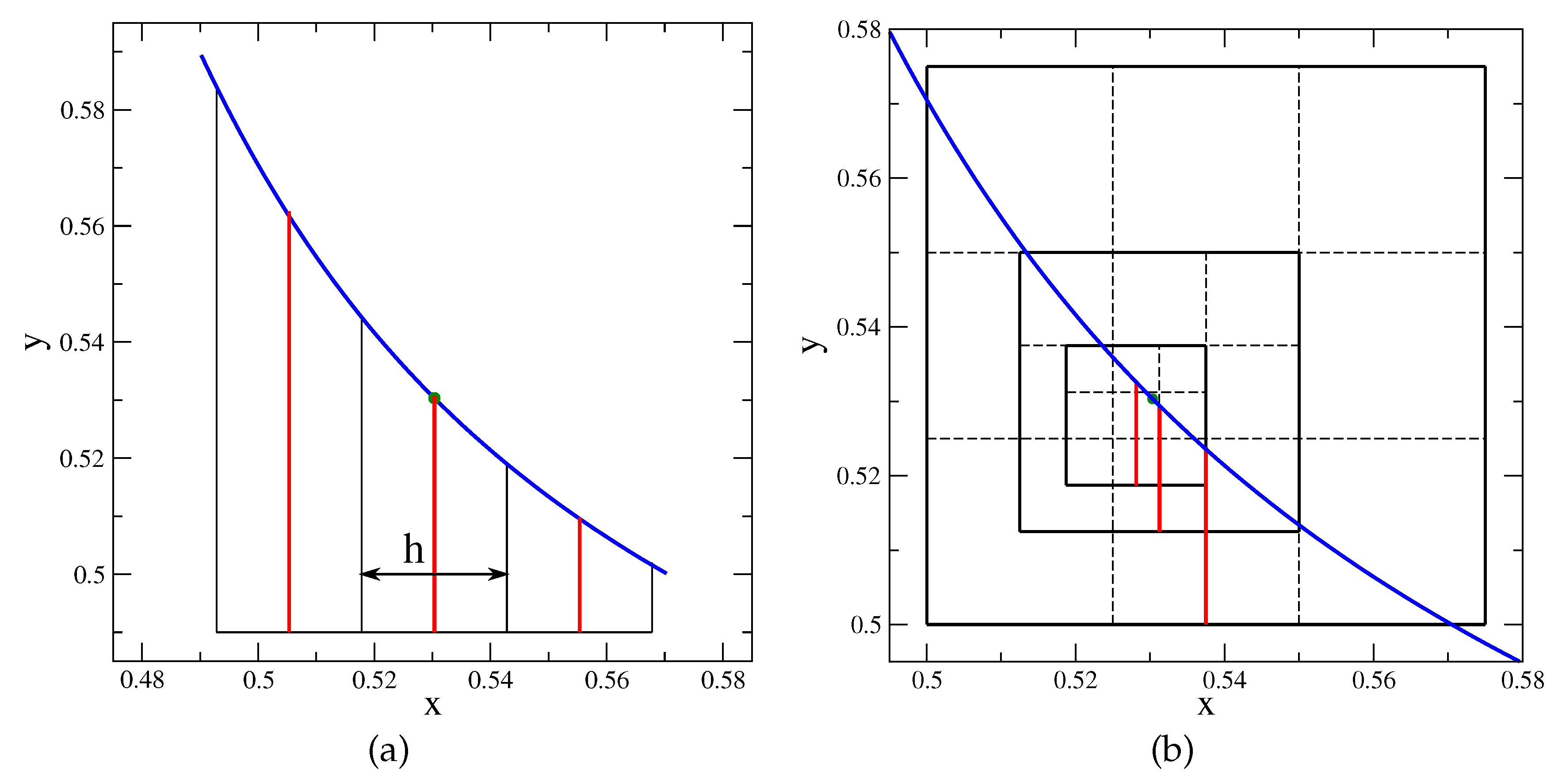
Figure 5.
Local error at point at the different resolutions : (a) first derivative, and (b) curvature. The errors , and are defined in the text.
Figure 5.
Local error at point at the different resolutions : (a) first derivative, and (b) curvature. The errors , and are defined in the text.
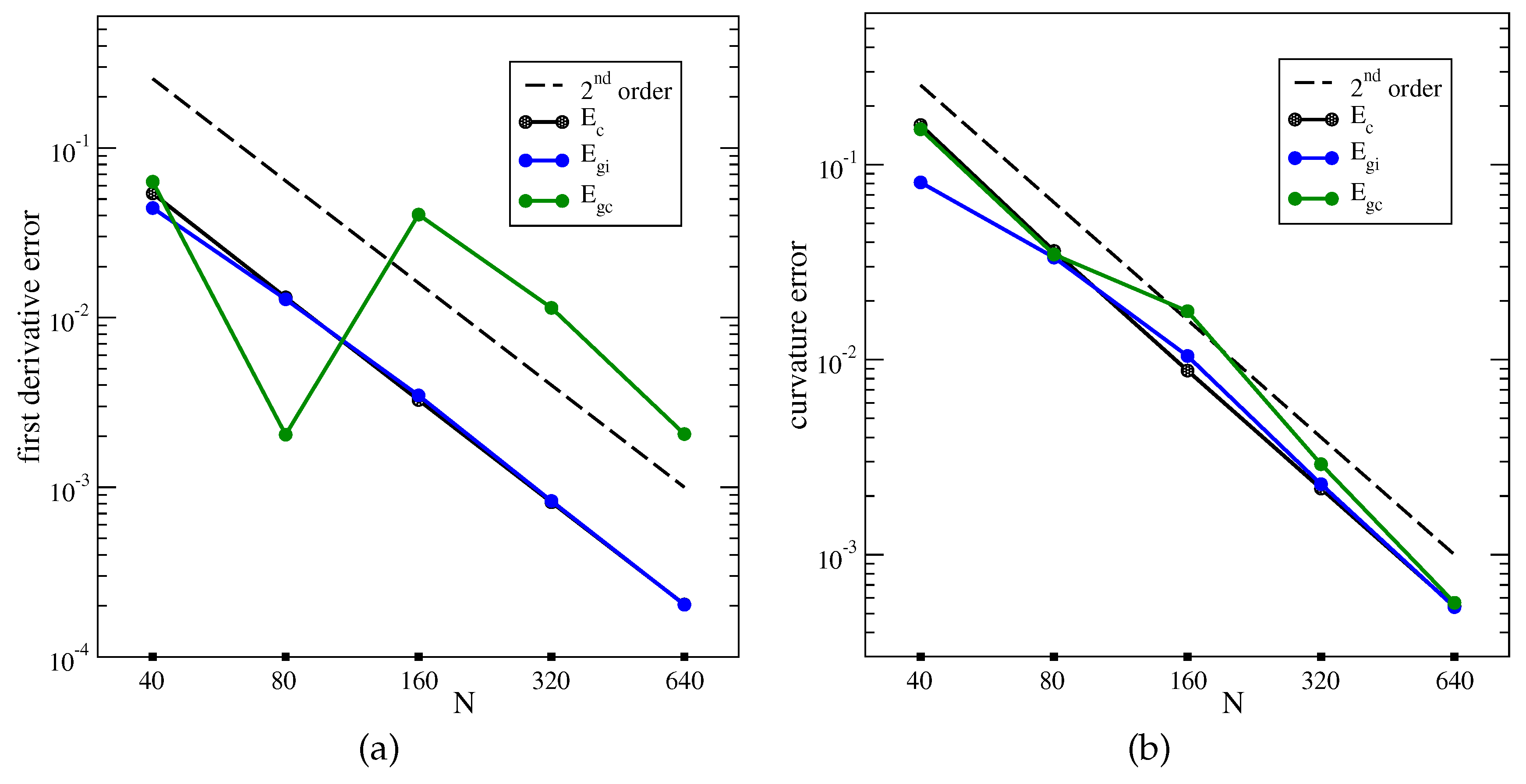
Figure 6.
Local error as s function of the angle , at the different grid resolutions N (): (a) height function, (b) first derivative, (c) second derivative and (d) curvature.
Figure 6.
Local error as s function of the angle , at the different grid resolutions N (): (a) height function, (b) first derivative, (c) second derivative and (d) curvature.
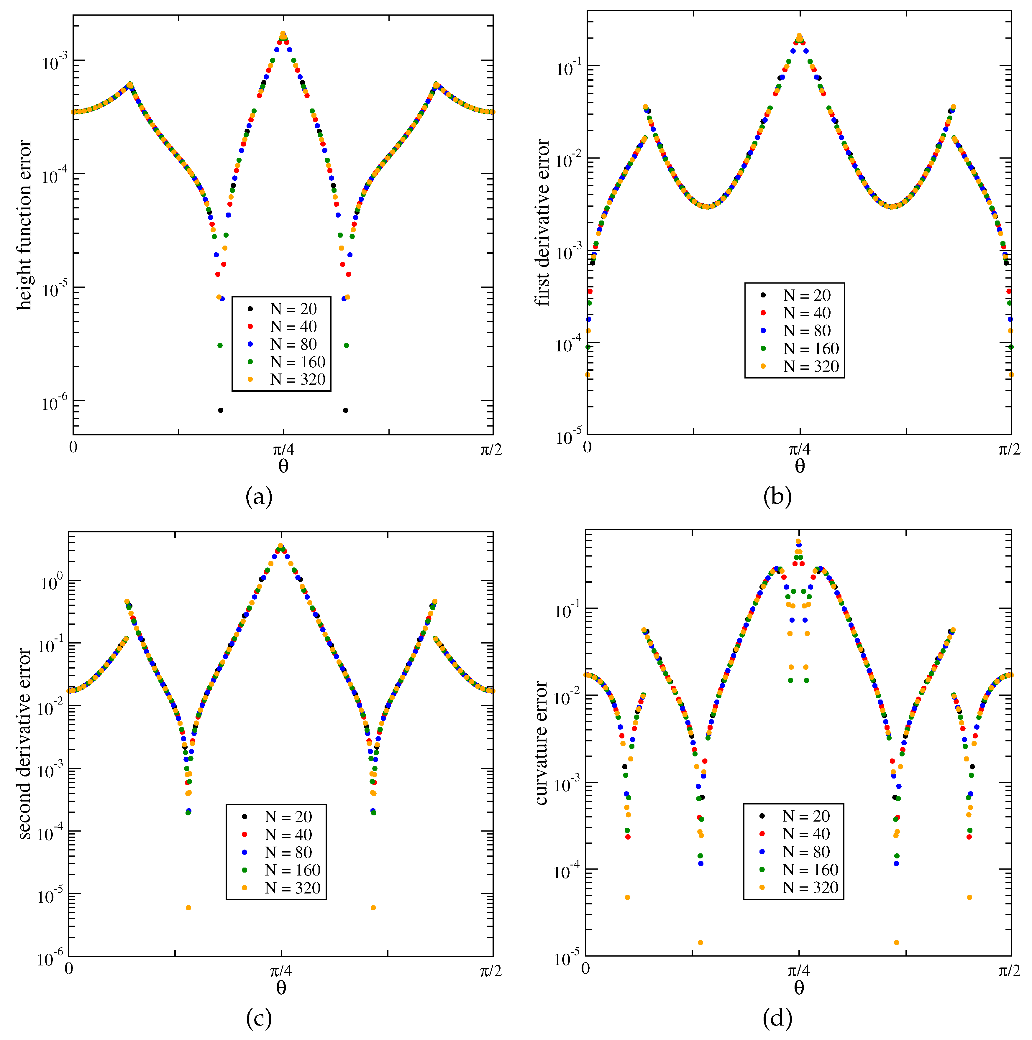
Figure 7.
Convergence of and error norms as a function of the grid resolution N: (a) first derivative, (b) curvature.
Figure 7.
Convergence of and error norms as a function of the grid resolution N: (a) first derivative, (b) curvature.
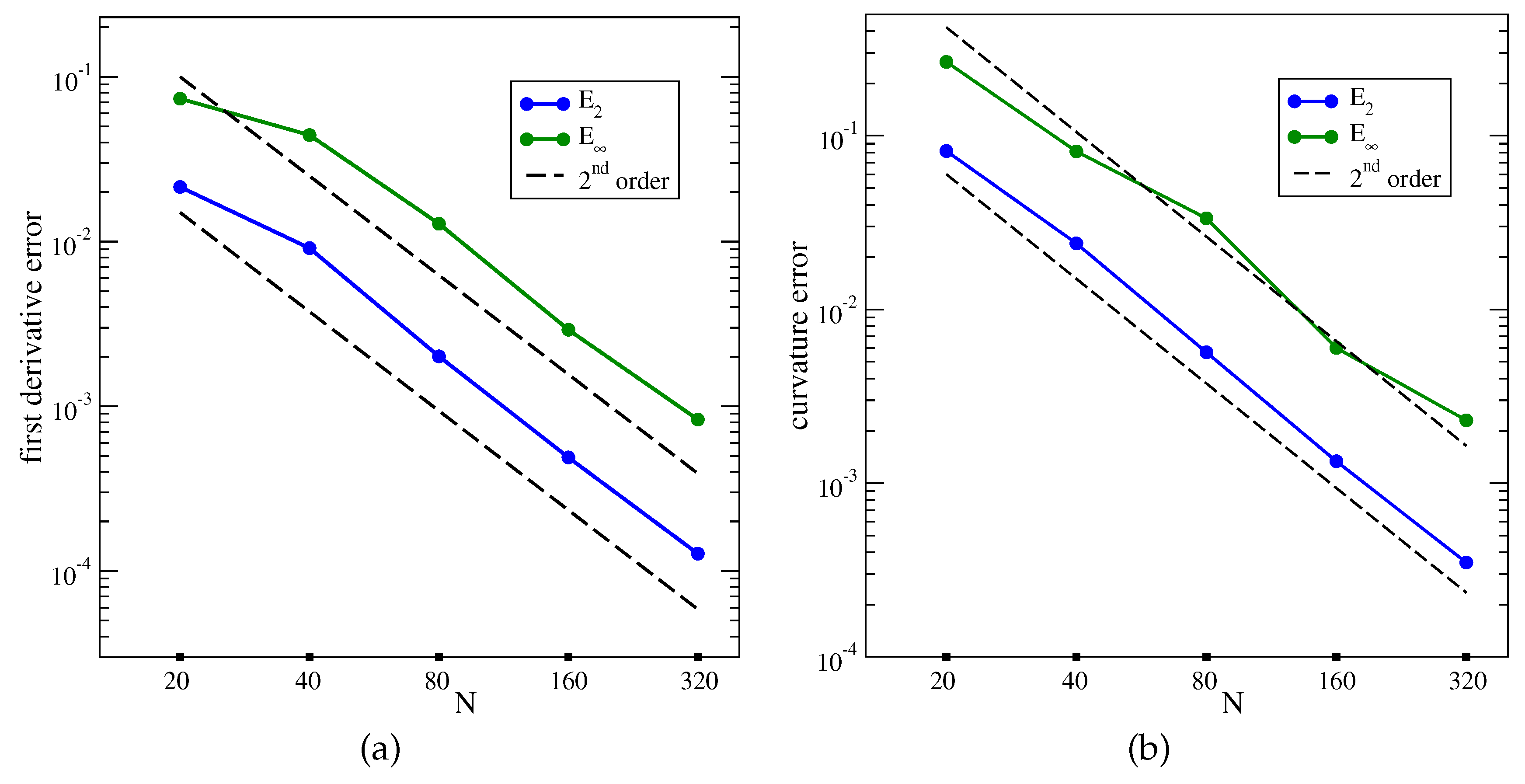
Figure 8.
Convergence of the constant, linear, and quadratic interpolations of the first derivative as a function of the grid resolution N: (a) error norm, (b) error norm.
Figure 8.
Convergence of the constant, linear, and quadratic interpolations of the first derivative as a function of the grid resolution N: (a) error norm, (b) error norm.
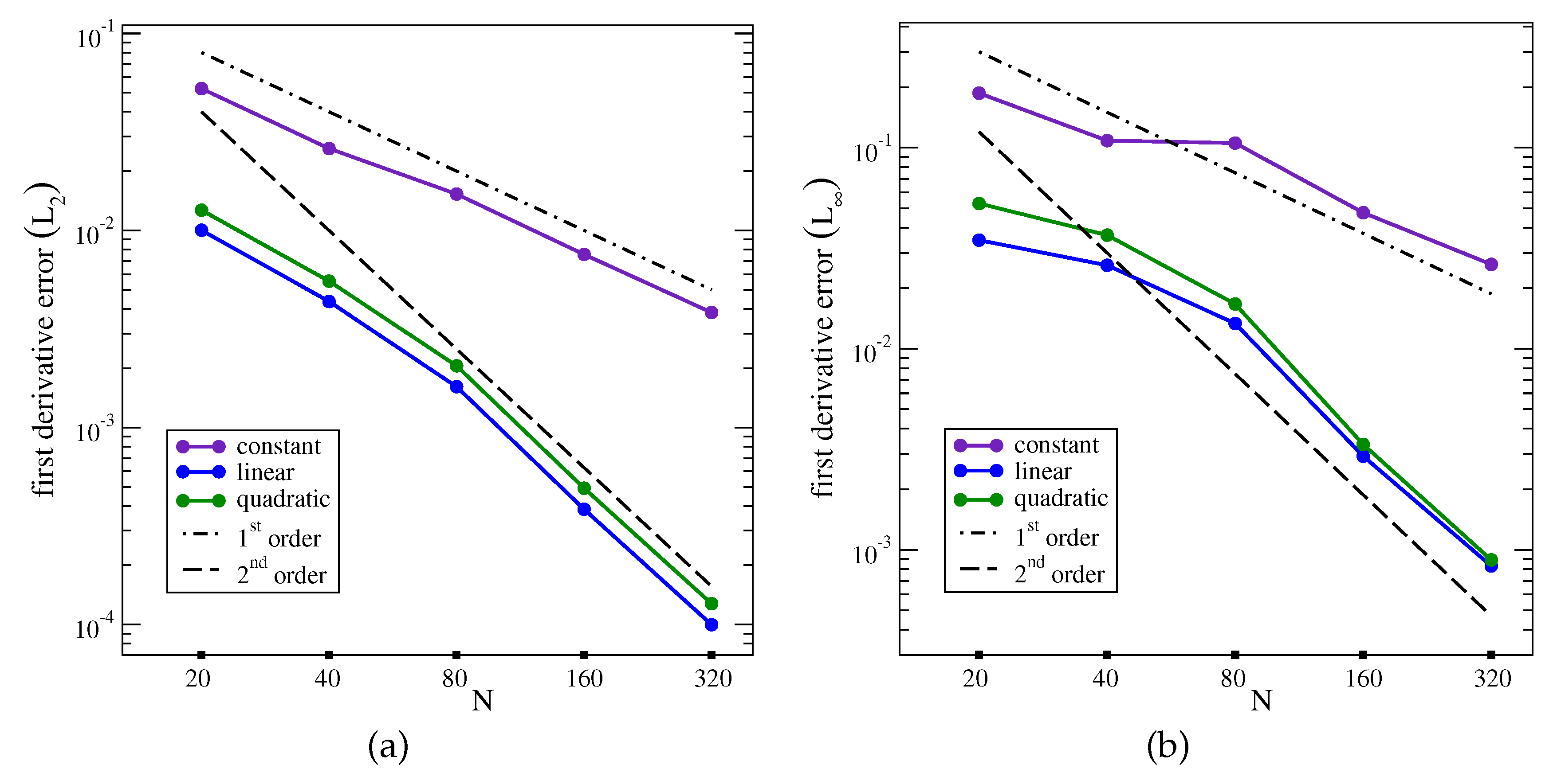
Figure 9.
Convergence of the constant, linear, and quadratic interpolations of the curvature as a function of the grid resolution N: (a) error norm, (b) error norm.
Figure 9.
Convergence of the constant, linear, and quadratic interpolations of the curvature as a function of the grid resolution N: (a) error norm, (b) error norm.
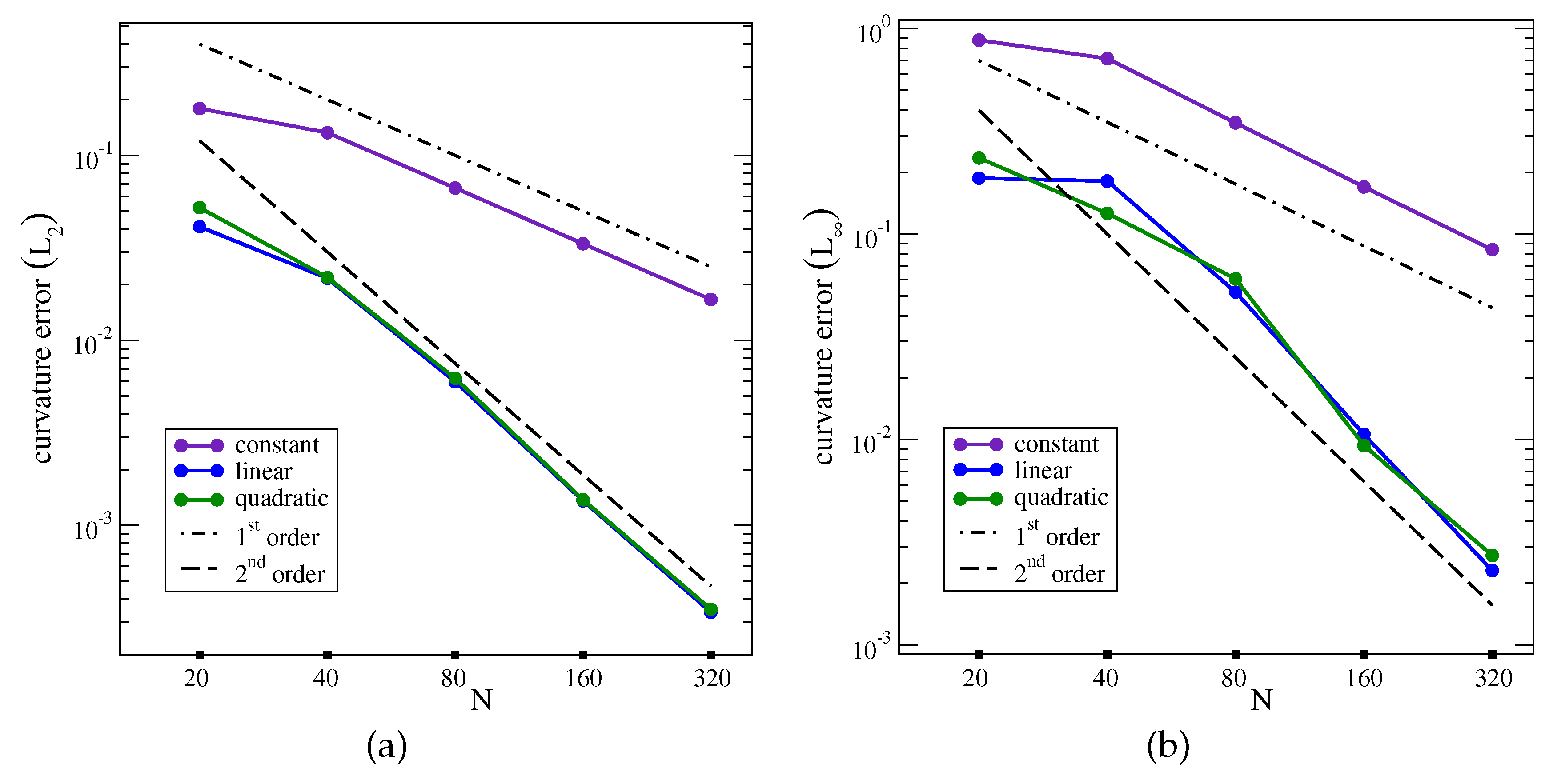
Figure 10.
Linear and quadratic interpolations in a vertical column at the coarsest resolution : (a) interface line; (b) curvature. The marks * are at abscissa x of the 8 additional points where we compute the error between the two interpolations and the analytical curve.
Figure 10.
Linear and quadratic interpolations in a vertical column at the coarsest resolution : (a) interface line; (b) curvature. The marks * are at abscissa x of the 8 additional points where we compute the error between the two interpolations and the analytical curve.
Disclaimer/Publisher’s Note: The statements, opinions and data contained in all publications are solely those of the individual author(s) and contributor(s) and not of MDPI and/or the editor(s). MDPI and/or the editor(s) disclaim responsibility for any injury to people or property resulting from any ideas, methods, instructions or products referred to in the content. |
© 2025 by the authors. Licensee MDPI, Basel, Switzerland. This article is an open access article distributed under the terms and conditions of the Creative Commons Attribution (CC BY) license (http://creativecommons.org/licenses/by/4.0/).
Copyright: This open access article is published under a Creative Commons CC BY 4.0 license, which permit the free download, distribution, and reuse, provided that the author and preprint are cited in any reuse.


