Submitted:
10 April 2025
Posted:
10 April 2025
You are already at the latest version
Abstract
The phase fraction plays a critical role in determining the solidification characteristics of metallic alloys. In this study, we propose a simplified method for estimating phase fraction based on the solidification time in cooling curves. The method was validated through experimental analysis of Al-18wt%Cu and Fe42Ni42B16 alloys, where phase fractions derived from cooling curves were compared with quantitative microstructure evaluations using computer-aided image analysis and the box-counting method. Results demonstrate strong consistency between the estimated phase fractions and experimental measurements, confirming the method’s reliability. The present method is easier operating, since it does not need derivative and integrals operations compared to Newtonian thermal analysis and Fourier thermal analysis methods. Furthermore, two key relationships deduced from the cooling curves were identified and analyzed: V/Rc=D/ΔT and RΔt=constant. These findings establish an operational framework for quantifying phase fractions and solidification rates in rapid solidification.
Keywords:
phase fraction
; cooling curve
; microstructure
; solidification
1. Introduction
The phase fraction analysis is useful to adjust the process for the material microstructure and properties controlling [1]. Neutron transmission spectroscopic imaging has enabled quantitative analysis of solid-liquid phase evolution during solidification through Bragg-edge profile analysis [2]. This wavelength-resolved technique has been further extended to characterize martensite phase fractions in bulk ferritic steels [3]. While X-ray computed tomography provides alternative phase quantification capabilities [4], and solidification phase fraction correlations have demonstrated predictive value for mechanical properties in additively manufactured Ti-6Al-4V alloys [5], these advanced characterization methods remain constrained by high operational costs and technical complexity. However, the temperature curve of alloy solidification process is helpful to obtain the phase fraction quickly and low cost, which has been used to study the process effect alloying elements on the mechanical performance of alloys [6]. There are several methods determine the phase fraction from temperature curve such as differential scanning calorimeter (DSC) [7], differential thermal analysis (DTA) microstructure [8,9], cooling curve thermal analysis [10,11], and baseline method [12]. Techniques like DTA and DSC are used for laboratory testing and cannot be used in the cases far from ideal and non-equilibrium system [13]. Cooling curve thermal analysis is regarded as one of the most effective methods for online monitoring of molten metal solidification processes, with two methods: Newtonian thermal analysis [14] and Fourier thermal analysis [15]. Both of these methods involve deriving the cooling curve and then integrating it [14,15]. Newtonian thermal analysis is using only one thermocouple that is centered in a solidifying sample, where the sample is assumed to be spatially isothermal. The most basic zero curve is an exponential that is fitted to the derivative of the cooling curve in the solid region [16]. However, due to differing heat capacities between the liquid and the solid, the zero curve rarely fits the derivative of the cooling curve in the liquid region too. For Fourier analysis it also uses a zero curve and the relative area between the zero curve and the derivative of the cooling curve to calculate solid fraction [15]. The difference between Fourier and Newtonian analysis is in how data are gathered and how the zero curve is determined. Data collection for the Fourier method utilizes two thermocouples of known locations in the sample; this allows the thermal gradient of the sample to be calculated. The thermal gradient along with thermal diffusivity, which is calculated from the cooling curve, is used to create a zero curve. The two methods require derivative and integral operations, so that it is not easy to operate. Furthermore, after derivation of some temperature curve with particularly dense collected data, the obtained curve fluctuates greatly, and the baseline cannot be found sometimes. Xu et al. report a baseline method [12] which uses the extension line of the liquid phase and the solid phase line as the baseline. It can avoid the problem of derivation cooling curve, but, this extension line is extended too far sometimes from the experiment data, with great uncertainty, and the extension line equation is not easy to determine accurately.
In the cooling curve of alloy undercooled solidification, there is a solidification plateau time, which was studied early by W. C. Roberts-Austen in 1897 [17]. After that, there are many studies focus on the recalescence process of undercooled solidification [18,19,20,21,22,23]. Patel et al. gave a method for handling the rapid solidification recalescence in laser spot welding by solving the coupled transient conservation equations of mass, momentum and energy [18]. He et al. studied the recalescence curves of rapid solidification of invar alloy and found that with the solidification of undercooling increasing, the microstructure changes from large dendrites to small columnar grains and then to fine equiaxed grains [19]. Galenko et al. studied the anomalous kinetics, patterns formation in recalescence, and found that changes in the shape of the recalescence front as the growth front morphology occur and multiple nucleation events forming the growth front [20]. An et al. studied the effect of Co on solidification characteristics and microstructural transformation of nonequilibrium solidified Cu-Ni alloys and found that the addition of a small amount of Co weakens the recalescence behaviour of the Cu55Ni45 alloy and significantly reduces the thermal strain in the rapid solidification phase [21]. Yang et al. studied the maximal recalescence temperature TR upon rapid solidification of bulk undercooled Cu 70 Ni 30 alloy and found that TR is affected by the difference of Gibbs free energy between the residual liquid and solid after recalescence [22]. Mullis et al. studied Why re-melting is not a plausible explanation in Ag-Cu alloy, and found that at low undercooling the volume fraction of anomalous eutectic near the nucleation site is around an order of magnitude greater than the calculated recalescence solid fraction [23]. Despite so many reports about recalescence, there is still a lack of systematic reports on the solidification fraction, solidification rate and solidification plateau time.
As the heat absorption in the solidification process for liquid and solid does not vary significantly, all the transition heat must be dissipated from the sample surface, and the heat release time for liquid and solid phases can be considered equivalent for the same size sample. Based on that, we propose a new method to quickly estimate the solid fraction during solidification upon the heat release time in this study. This approach eliminates computational dependencies while maintaining operational simplicity. Then the validation is conducted through synchronized cooling curve analysis and microstructural characterization of Al-18wt%Cu and Fe42Ni42B16 alloys. After that the solidification fraction, solidification rate and solidification plateau time will be discussed further.
2. Methods Description
2.1. Phase Fraction Prediction Method
The method is demonstrated in Figure 1, example for a typical cooling curve with two transitions in solidification. If one sample was cooled from high temperature to room temperature with liquid state (never solidified), the cooling process should be from A to B. If a solid sample that was not melted at high temperatures is cooled to room temperature, the temperature curve should change from point C to point D, as shown in Figure 1. The actual process that the sample’s temperature changes from high to low, the liquid phase transforms to a solid phase, so the temperature curve is changing along AB to CD gradually. Thus, AB and CD can be seen as the baseline for liquid and solid phase respectively. To estimate the solid phase faction during solidification and the method should not be difficult to operate, so the baseline AB and CD can be fitted by a parabolic equation. The detailed process for solid fraction calculation can be described as:
① Fitting the pure solid phase part of the cooling curve CD by a parabolic equation.
② Because the specific heat of the liquid and solid phases of the same sample is slightly different, different equations should be used for the cooling rates of the solid and liquid phases at the same temperature. The overall shapes of AB and CD are similar, so we can use the parabolic equation with the same quadratic coefficient α from Equation (1) to fit the liquid phase region of the cooling curve AB.
③ Then if a suitable equation can be used to describe the experiment data, it can be expressed as
T=T(t)
Note that all the equations above correspond to a single value of temperature and time.
④ The solid phase fraction of each point on the cooling curve is can be estimated by
The process is as shown in Figure 1. For any time t, the corresponding temperature T on the experimental data curve can be found by Equation (3). And then with the same T, we can calculate ts and tl from Equation (1) and Equation (2), respectively. In this way, the solid phase fraction for each temperature and time can be determined through Equation (4).
2.2. Microstructure Measurement Method
To identify the predicted result, there are two methods to measure the phase fraction from microstructure image. One method is computer aid image analysis which has been described by Gandin et al. [24]. It is based on a binary representation derived from microstructure images. For this method, the sample must be corroded well with a suitable etchant, and then the phase fraction can be accurately obtained by having a high contrast between the two phases in the photograph. When the microstructure images are of insufficient quality, this method cannot be used.
The second method is box-counting method improved by Xu et al.[25], which can solve the measurement difficulties caused by low image quality and uneven color distribution. It can be described as covered the image by the boxes of L×L at first, then the boxes containing primary phase (including boxes full of primary phase and the others partially filled with primary phase) is counted as α, and the boxes only contains primary phase is counted as αf. Then the fraction of the primary phase can be obtained by [25]
Equation (5) will give a more accurate result if the box size is smaller than the aim phase size, and the error analyzed details can be found in Ref. [25].
3. Experimental
In order to verify the present method, experimental data of Al-Cu and Fe-Ni-B alloys are analyzed. Figure 2a is the cooling curve measured from the solidification of an Al-18wt%Cu alloy sample. Then with the method described in Section 2, the pure solid phase part of the cooling curve can be fitted as =1.48t2-531.48t+47545.25. The pure liquid phase part can be fitted as =1.48 t2-493.80t+41625.85. Then from Equation (4) we can obtain the solid phase fraction curves of f-t (Figure 2a) and T-t (Figure 2b). From the inflection point of the curve, the fraction of primary phase dendrites (α-Al) is determined as 67%.
Figure 2c shows the SEM microstructure of the Al-18wt%Cu alloy sample. By adopting the computer image segmentation method, we can obtain the binary image as shown in Figure 2d, and the dendrite phase fraction is determined by the area of the red region as 65%. At the present, 67% or 65%, there is no way to prove which result is more accurate because the microstructure is only shown in the fraction of the section. That is to say, the calculation error from the cooling curve comes from the difference in the specific heat of the solid and liquid phases, and the error from the microstructure photos comes from the difference between the cross-sectional fraction and the real phase volume fraction. Whereas the results obtained from Equation (5) are in close agreement with the microstructure measurements.
To further validate the time fraction method derived from cooling curves, Figure 3a presents the cooling curves of the Fe₄₂Ni₄₂B₁₆ alloy. By using Equations (1)-(4), we can calculate the solid fraction curve f-t. From the eutectic transition point (the inflection point of solid fraction curve), we can determine the primary phase α-Fe(Ni) as about 0.335. The corresponding microstructure is shown in Figure 3b. For this microstructure, because the color distribution is not uniform and the score cannot be obtained by computer image analysis, so we adopt the box-counting method studied by Xu et al. [25]. The microstructure image in Figure 3b is covered by boxes of 50×50. The first step is counting the number of the full box as αf=473 (Figure 3c). The second step is counting the number of full and half boxes as α=1170 (Figure 3d). The total box number is 2500. Then by using Equation (5), the value of the primary phase α-Fe(Ni) fraction is obtained as f=(αf+α)/2L2=(473+1170)/2×50×50=0.328, which is very near the predicted result (0.335) from cooling curve. This method is not quickly but more reliable, which has been discussed in Ref. [25]. Therefore, the present method can be used to estimate the solid fraction during solidification.
4. Discussions
4.1. Solidification Fraction
Our previous study shows that the cooling curve can be calculated from the high-speed photographs of the solidification process [26], combining the present study results, the solid fraction can be estimated from the high-speed photographs directly, i.e., obtained the cooling curve from the high-speed video first, then analyzed the phase fraction from the cooling curve based on Equation (4). In this way, high-speed photography enables not only the quantitative tracking of solid-liquid interface velocity and morphology dynamics but also the calculation of solid phase fractions during solidification. When all the parameters are acquired from a single device, the time correspondence should be better than that from multiple device measurements. Therefore, a more complete solidification theoretical model can be developed based on these techniques.
4.2. Solidification Rate
Besides the solidification fraction related with cooling curve, the solidification rate, and the cooling rate can also be estimated from the cooling curves, as shown in Figure 5. Given Δτ as the time between recalescence start point and finish point, it can be expressed as:
Δτ=D/V=ΔT/Rc
Where D is the diameter of temperature measurement range which is determined by the parameter of the thermometer itself. V is the velocity of the solidification interface. Rc is the recalescence rate, Rc=ΔTR/Δτ, where ΔTR is the recalescence height in the temperature curve (Figure 5). Then, the relation between the solidification rate and recalescence rate in cooling curve can expressed as:
V/Rc=D/ΔT
This relation can be used to estamted the solidificaition rate from cooling curves.
4.3. Solidification Plateau Time
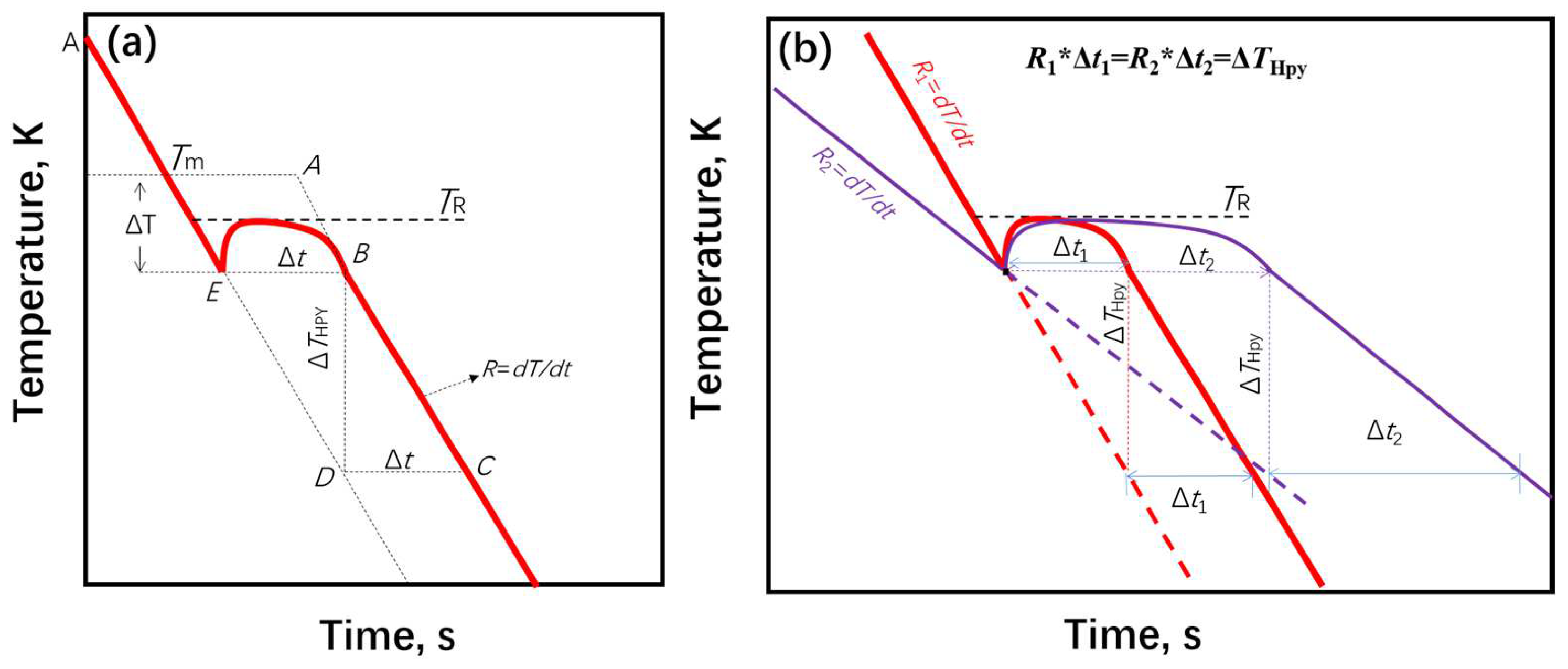
There is another relation between cooling rate and solidification plateau time (Δt) in cooling curve. Figure 6a shows the schematic diagram of the thermal history of a metallic sample in solidification process. For convenience of study, assumed the specific heat (Cp) is a constant so that the cooling curve can be seen as straight before or after solidification. As BC//ED, if we move BC to ED, where the point E can be seen as the nucleation point, it is easy to obtain the relationship from based on geometric knowledge,
where R is the cooling rate(=dT/dt), Δt the solidification plateau time from point E to B. Eq.(8) indicates that for an alloy, the cooling rate and the solidification plateau time is
BD=RΔt
RΔt =constant
If we assumed that there was no latent heat release in solidification, the thermal history may go along with the AED from liquid phase to solid phase. Because the latent heat of alloy in solidification is released that the temperature of the sample will increase or decrease at the same rate as the cooling rate, and the thermal history of the sample follows the path of AEBC (Figure 6a). At a time t, without consider the latent heat, the system temperature is D, and due to the latent heat release, the system temperature is B. Therefore, in the same time the temperature difference of D and B is attributed to the latent heat work, so there is
BD=⊿H/Cp=⊿Thpy
ΔTHpy is the temperature rise due to all the latent heat release. From Equation (8) and Equation (10), we have
RΔt =BD=⊿Thpy
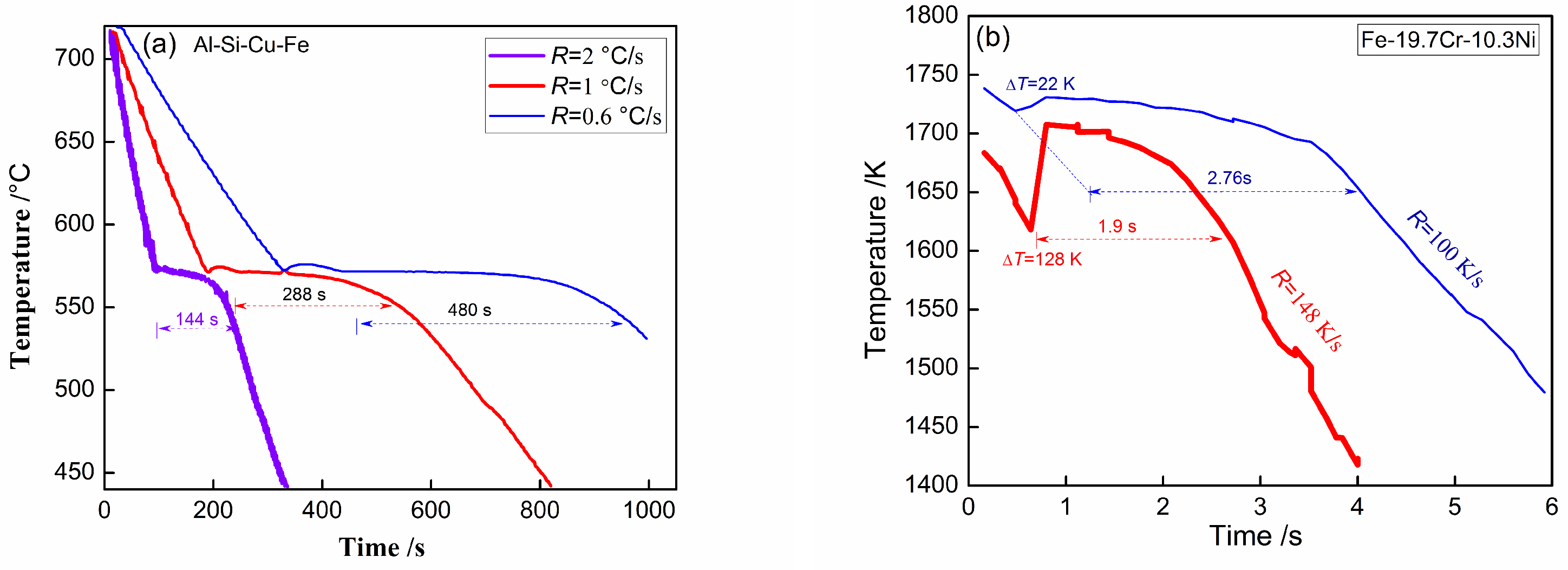
From Equation (11), the solidification plateau time is decided by cooling rate. The larger the cooling rate, the longer the solidification plateau time (Δt) is as shown in Figure 6b. we can find many experiment reports showing this rule [27,28]. Figure 7(a) displays the temperature curves during solidification of Al–Si–Cu–Fe alloy under varying cooling rates [26]. It can be found that for the curves with cooling rates of 2 °C/s, 1 °C/s, 0.6 °C/s, the corresponding plateau times are about 144 s, 288 s, 480 s, confirming the validity of the relationship RΔt=constant. Similarly, Figure 7(b) presents the cooling curves obtained during rapid solidification of Fe-Ni-Cr alloys with different undercoolings [28], which further corroborates the relationship of RΔt = constant in solidification processes.
The heating process also follows a similar relationship as Equation (9) which is not discussed here. Equations (4), (7) and (9) are three simple relationships for cooling curves of alloy in solidification.
5. Conclusions
From the cooling curve of the rapid solidification sample, the phase fraction change can be estimated using the proposed method based on the heat release time (). Its accuracy and practical applicability were validated through analyses of cooling curves and microstructures in Al-Cu and Fe-Ni-B alloys. The results were further corroborated by computer-aided image analysis and the box counting method for microstructural characterization. Unlike Newtonian thermal analysis and Fourier thermal analysis, which require derivative and integration operations, the present method offers greater operational simplicity. Additionally, two key relationships were identified from the cooling curves: the growth velocity–recalescence (V/Rc=D/ΔT) and the cooling rate–solidification plateau time (RΔt=constant). These relationships, combined with the phase fraction estimation, enable the prediction of solidification microstructure and solidification rate in rapid solidification processes.
Author Contributions
Conceptualization, Junfeng Xu; Methodology, Junfeng Xu, Tian Yang and Changlin Yang; Software, Junfeng Xu and Tian Yang; Validation, Junfeng Xu; Formal analysis, Yindong Fang and Changlin Yang; Investigation, Junfeng Xu; Data curation, Yindong Fang and Tian Yang; Writing—original draft, Junfeng Xu; Writing—review & editing, Junfeng Xu and Changlin Yang; Project administration, Junfeng Xu; Funding acquisition, Junfeng Xu.
Acknowledgments
The present work is dedicated to the blessed memory of Professor Markus Rettenmayr who provided thorough thermodynamic study and practical applications for novel metallic and alloying materials. JF Xu thank Professor Peter K. Galenko, Zhuo Li and Jitao Cao for their help with this study. This study is supported by National Natural Science Foundation of China (6220419).
References
- Tang, P.; Hu, Z.; Zhao, Y.; Huang, Q. Investigation on the solidification course of Al–Si alloys by using a numerical Newtonian thermal analysis method. Mater. Res. Express 2017, 4, 126511. [Google Scholar] [CrossRef]
- Kamiyama, T.; Hirano, K.; Sato, H.; Ono, K.; Suzuki, Y.; Ito, D.; Saito, Y. Application of Machine Learning Methods to Neutron Transmission Spectroscopic Imaging for Solid–Liquid Phase Fraction Analysis. Appl. Sci. 2021, 11, 5988. [Google Scholar] [CrossRef]
- Sato, H.; Kusumi, A.; Shiota, Y.; Hayashida, H.; Su, Y.; Parker, J.D.; Watanabe, K.; Kamiyama, T.; Kiyanagi, Y. Visualising Martensite Phase Fraction in Bulk Ferrite Steel by Superimposed Bragg-edge Profile Analysis of Wavelength-resolved Neutron Transmission Imaging. ISIJ Int. 2022, 62, 2319–2330. [Google Scholar] [CrossRef]
- Guarda, D.; Martinez-Garcia, J.; Fenk, B.; Schiffmann, D.; Gwerder, D.; Stamatiou, A.; Worlitschek, J.; Mancin, S.; Schuetz, P. New liquid fraction measurement methodology for phase change material analysis based on X-ray computed tomography. Int. J. Therm. Sci. 2023, 194, 108585. [Google Scholar] [CrossRef]
- Kamath, R.R.; Nandwana, P.; Ren, Y.; Choo, H. Solidification texture, variant selection, and phase fraction in a spot-melt electron-beam powder bed fusion processed Ti-6Al-4V. Addit. Manuf. 2021, 46, 102136. [Google Scholar] [CrossRef]
- Cruz, H.; Gonzalez, C.; Juárez, A.; Herrera, M.; Juarez, J. Quantification of the microconstituents formed during solidification by the Newton thermal analysis method. J. Mech. Work. Technol. 2006, 178, 128–134. [Google Scholar] [CrossRef]
- Schumacher P, Pogatscher S, Starink M J, SchickC, Mohles V and Milkereit B 2015 Quench-induced precipitates in Al–Si alloys: calorimetric determination of solute content and characterisation of microstructure Thermochim. Acta 602 63–73.
- Hernandez FCR and Sokolowski J H 2006 Thermal analysis and microscopical characterization of Al–Si hypereutectic alloys J. Alloys Compd. 419 180–90.
- Farahany S, Idris M H, OurdjiniA, Faris F and Ghandvar H 2015 Evaluation of the effect of grain refiners on the solidification characteristics of an Sr-modified ADC12 die-casting alloy by cooling curve thermal analysis J. Therm. Anal. Calorim. 119 1593–601.
- Fras, E. , Kapturkiewicz, W., Burbielko, A., & Lopez, H. F. (1993). A new concept in thermal analysis of castings. Transactions of the American Foundrymen’s Society., 101, 505-511.
- Emadi, D.; Whiting, L.V.; Djurdjevic, M.; Kierkus, W.T.; Sokolowski, J. Comparison of Newtonian and Fourier thermal analysis techniques for calculation of latent heat and solid fraction of aluminum alloys. Met. Met. 2004, 10, 91–106. [Google Scholar] [CrossRef]
- Xu, J.; Liu, F.; Xu, X.; Chen, Y. Determination of Solid Fraction from Cooling Curve. Met. Mater. Trans. A 2011, 43, 1268–1276. [Google Scholar] [CrossRef]
- Dediaeva E, PadalkoA, Akopyan T, SuchkovA and FedotovV 2015 Barothermography and microstructure of the hypoeutectic and eutectic alloys in Al–Si system J. Therm. Anal. Calorim. 121 485–90.
- J.W. Gibbs, M.J. Kaufman, R.E. Hackenberg, and P.F. Mendez: Metall. Mater. Trans. A, 2010, vol. 41A, pp. 2216–23.
- Djurdjevic M B, Odanovic Z, Talijan N. Characterization of the solidification path of AlSi5Cu (1–4 wt.%) alloys using cooling curve analysis[J]. Jom, 2011, 63(11): 51-57.
- D.M. Stefanescu, G. Upadhya, D. Bandyopadhyay, Metall. Trans. A 21A (1990) 997–100.
- Surfusion in Metals and Alloys1. Nature 1898, 58, 619–621. [CrossRef]
- Patel, S.; Reddy, P.; Kumar, A. A methodology to integrate melt pool convection with rapid solidification and undercooling kinetics in laser spot welding. Int. J. Heat Mass Transf. 2021, 164, 120575. [Google Scholar] [CrossRef]
- He, H.; Yao, Z.; Li, X.; Xu, J. Rapid Solidification of Invar Alloy. Materials 2023, 17, 231. [Google Scholar] [CrossRef]
- Galenko, P.; Toropova, L.; Alexandrov, D.; Phanikumar, G.; Assadi, H.; Reinartz, M.; Paul, P.; Fang, Y.; Lippmann, S. Anomalous kinetics, patterns formation in recalescence, and final microstructure of rapidly solidified Al-rich Al-Ni alloys. Acta Mater. 2022, 241. [Google Scholar] [CrossRef]
- An, H.; Chua, B.-L.; Saad, I.; Liew, W.Y.H. Effect of Co on Solidification Characteristics and Microstructural Transformation of Nonequilibrium Solidified Cu-Ni Alloys. J. Wuhan Univ. Technol. Sci. Ed. 2024, 39, 444–453. [Google Scholar] [CrossRef]
- Yang, W.; Liu, F.; Wang, H.; Chen, Z.; Yang, G.; Zhou, Y. Prediction of the maximal recalescence temperature upon rapid solidification of bulk undercooled Cu70Ni30 alloy. J. Alloy. Compd. 2008, 470, L13–L16. [Google Scholar] [CrossRef]
- Mullis, A.M.; Clopet, C.R. On the origin of anomalous eutectic growth from undercooled melts: Why re-melting is not a plausible explanation. Acta Mater. 2018, 145, 186–195. [Google Scholar] [CrossRef]
- C. -A. Gandin, S. Mosbah, T. Volkmann, and D.M. Herlach: Acta Mater., 2008, 56, pp. 3023–35.
- Xu, J.; Jian, Z.; Lian, X. An application of box counting method for measuring phase fraction. Measurement 2017, 100, 297–300. [Google Scholar] [CrossRef]
- Xu, J.; Xiao, Y.; Jian, Z. Observe the temperature curve for solidification from high-speed video image. J. Therm. Anal. Calorim. 2021, 146, 2273–2277. [Google Scholar] [CrossRef]
- Farahany, S.; Ourdjini, A.; Idris, M.H.; Shabestari, S.G. Computer-aided cooling curve thermal analysis of near eutectic Al–Si–Cu–Fe alloy. J. Therm. Anal. Calorim. 2013, 114, 705–717. [Google Scholar] [CrossRef]
- Koseki Toshihiko. “Undercooling and rapid solidification of Fe-Cr-Ni ternary alloys.” Massachusetts Institute of Technology, 1994.4.
Figure 1.
Schematic diagram of phase fraction calculated method from time baseline. TL is the stage sample is full of liquid i.e., from “A” to “B” is curve TL(t). TL curve change (A to B) is due to specific heat of liquid phase change and the temperature difference between sample and environment. Ts curve (C to D) change is due to the specific heat of solid phase change and the temperature difference between sample and environment.
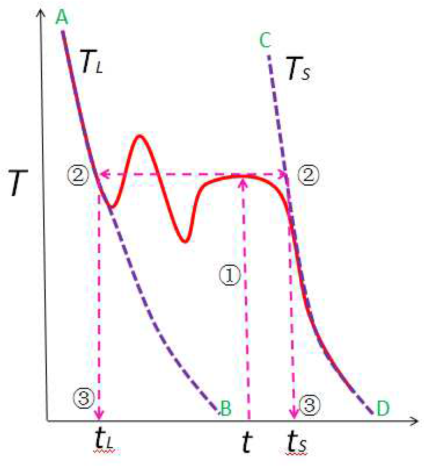
Figure 2.
Experiment and calculated result of Al-18wt%Cu alloy: (a) T-t curve and calculated f-t curve; (b) calculated f-T curve; (c) microstructure (The white area should be the eutectic region, but due to undercooled solidification, the eutectic area is replaced by single phase); (d) the primary phase fraction by computer image analysis(the green area is the eutectic region).
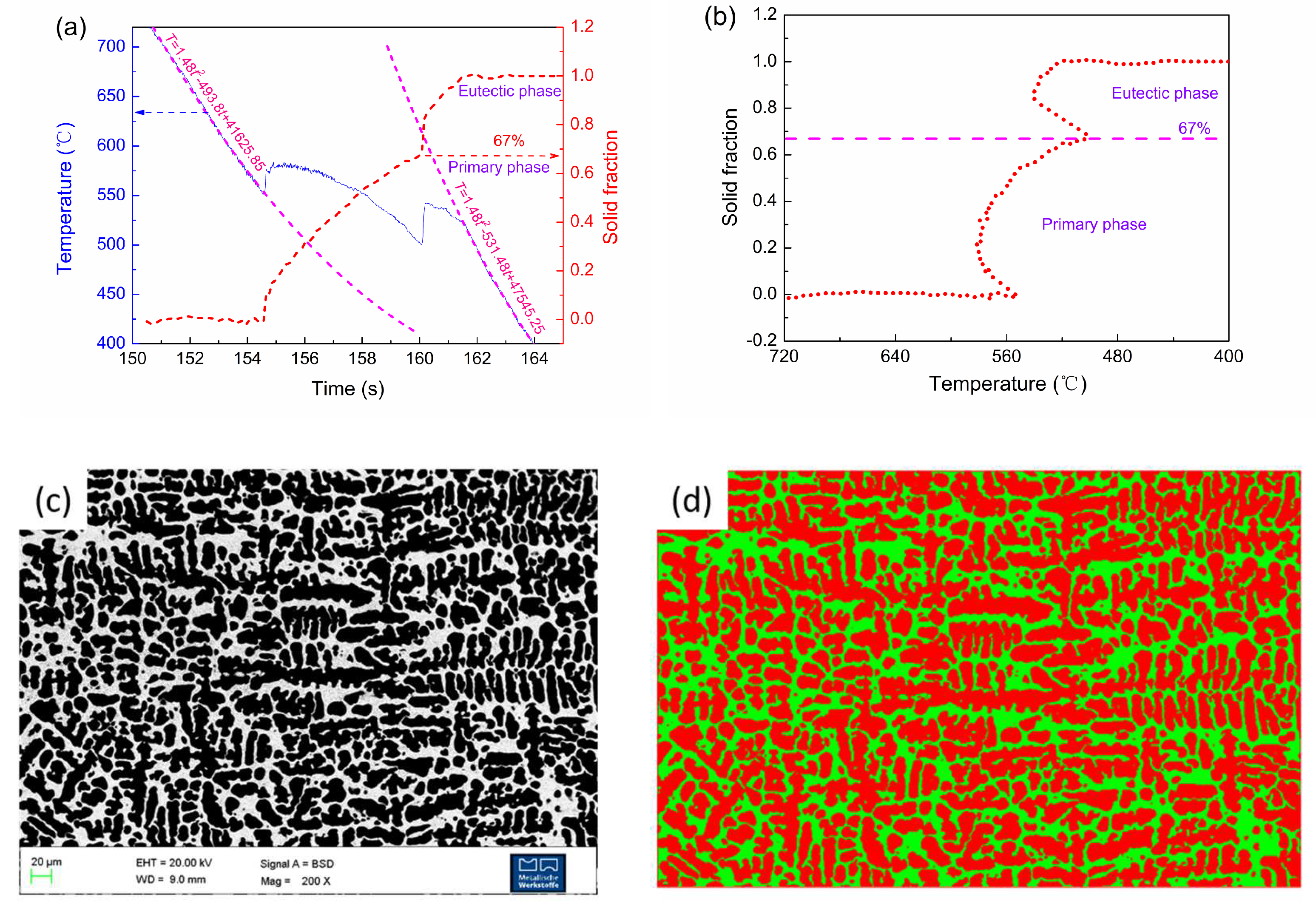
Figure 4.
Experiment and calculate result of Fe42Ni42B16 alloy: (a) T-t curve and f-t curves; (b) microstructure; (c) full box counting number αf=473; (d) half and full box counting number α=1170.
Figure 4.
Experiment and calculate result of Fe42Ni42B16 alloy: (a) T-t curve and f-t curves; (b) microstructure; (c) full box counting number αf=473; (d) half and full box counting number α=1170.
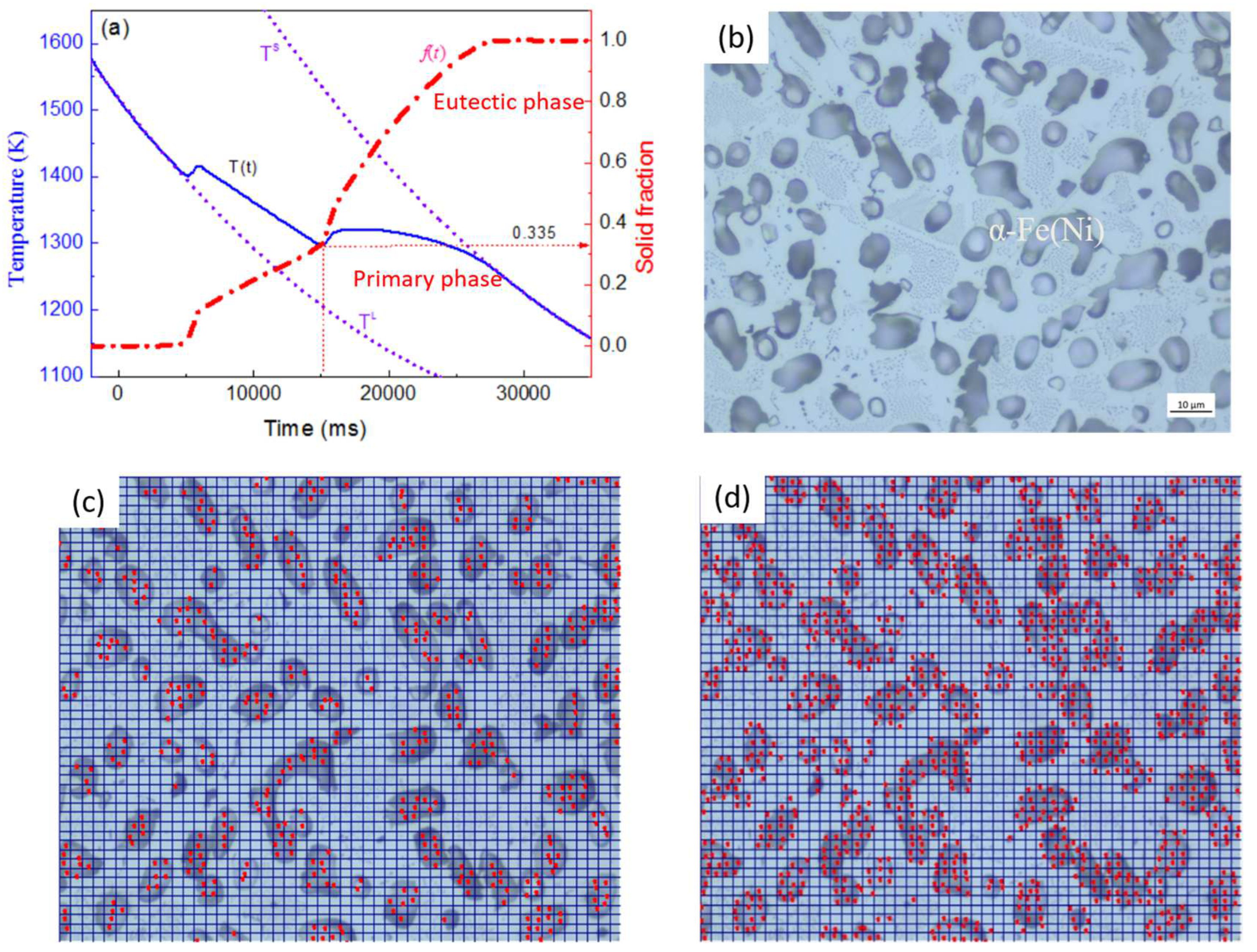
Figure 5.
The recalescence process vs. solidification process. D is the region diameter on the sample by the temperature detector. Δτ is the recalescence time.
Figure 5.
The recalescence process vs. solidification process. D is the region diameter on the sample by the temperature detector. Δτ is the recalescence time.
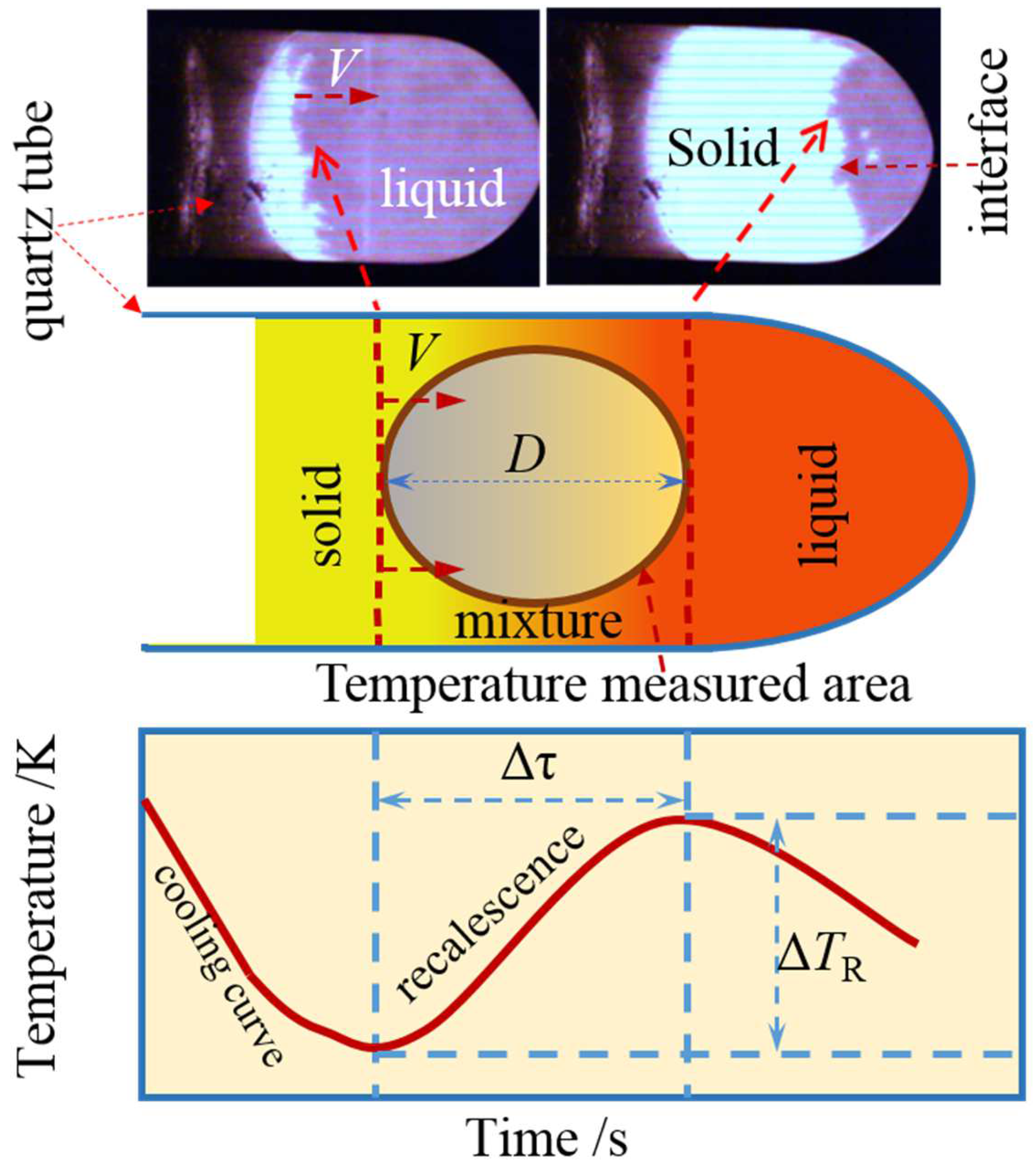
Figure 6.
Relation of solidification time(Δt) with cooling rate (R): (a) the cooling curve of the undercooled melt in solidification process; (b) cooling curves of alloys for different cooling rate.
Figure 6.
Relation of solidification time(Δt) with cooling rate (R): (a) the cooling curve of the undercooled melt in solidification process; (b) cooling curves of alloys for different cooling rate.
Disclaimer/Publisher’s Note: The statements, opinions and data contained in all publications are solely those of the individual author(s) and contributor(s) and not of MDPI and/or the editor(s). MDPI and/or the editor(s) disclaim responsibility for any injury to people or property resulting from any ideas, methods, instructions or products referred to in the content. |
© 2025 by the authors. Licensee MDPI, Basel, Switzerland. This article is an open access article distributed under the terms and conditions of the Creative Commons Attribution (CC BY) license (http://creativecommons.org/licenses/by/4.0/).
Copyright: This open access article is published under a Creative Commons CC BY 4.0 license, which permit the free download, distribution, and reuse, provided that the author and preprint are cited in any reuse.


