
Submitted:
08 April 2025
Posted:
08 April 2025
You are already at the latest version
Abstract
This study presents an innovative data-driven approach for the optimal design of water distribution networks (WDNs). The methodology comprises five key stages: Generation of 600 synthetic WDNs with diverse properties, optimized to determine optimal component diameters; Extraction of 80 topological and hydraulic features from the optimized WDNs using graph theory; Preprocessing and preparation of the extracted features using established data science methods; Application of six feature selection methods (Variance Threshold, k-best, chi-squared, Light Gradient-Boosting Machine, Permutation, and Extreme Gradient Boosting) to identify the most relevant features for describing optimal diameters; and Integration of the selected features with four machine learning models (Random Forest, Support Vector Machine, Bootstrap Aggregating, and Light Gradient-Boosting Machine), resulting in 24 ensemble models. The Extreme Gradient Boosting-Light Gradient-Boosting Machine (Xg-LGB) model emerged as the optimal choice, achieving R² and RMSE values of 0.98 and 0.02, respectively. When applied to a benchmark WDN, this model demonstrated high accuracy in predicting optimal diameters, with R² and RMSE values of 0.94 and 0.06, respectively. These results underscore the potential of the developed model for accurate and efficient optimal design of WDNs.
Keywords:
Water Distribution Networks
; Graph Theory
; Machine Learning
; Feature Engineering
; Network Optimization
1. Introduction
Water distribution networks (WDNs) are complex systems comprising interconnected components such as water supply sources, pipes, and control elements like pumps and valves. These networks play a crucial role in delivering water to consumers at the required pressure and quality. The design of WDNs has garnered significant attention from researchers and designers due to the substantial costs involved (Swamee and Sharma 2008).
The evolution of WDN design approaches has been marked by several key developments. Early efforts in the late 1960s focused on linear programming methods to minimize design costs under hydraulic constraints (Gupta 1969; Karmeli, Gadish, and Meyers 1968; Schaake and Lai 1969). The 1990s saw the rise of nonlinear programming techniques (Su et al. 1987, Duan et al. 1990, and Samani and Naeeni 1996). In recent years, metaheuristic algorithms have gained prominence for their ability to reduce costs effectively (Murphy and Simpson 1992; Savic and Walters 1997; Simpson, Dandy and Murphy 1994). As WDNs have grown more complex, multi-objective optimization algorithms have been developed to address additional factors such as reliability, water quality, and resilience (Creaco and Franchini 2014; Farmani, Walters and Savic 2005, 2006; Prasad and Park 2004; Riyahi, Bakhshipour and Haghighi 2023; Todini 2000).
Graph theory has emerged as a powerful tool for describing and analyzing WDNs. This approach represents WDNs as a set of nodes (consumers or hydraulic control components) connected by links (pipes) (Bondy and Murty 1976). The application of graph theory to WDNs began in the 1970s, initially focusing on understanding basic concepts and analyzing water flow and pressure (Hamam and Brameller 1971; Kesavan and Chandrashker 1972). Over time, researchers have adopted a more topological perspective, combining graph theory with analytical tools to develop innovative solutions for WDN analysis and design (Riyahi et al. 2024a).
Graph theory has found diverse applications in WDN research, including reliability analysis (Jung et al. 2016), network dimension reduction (Ulanicki et al. 1996; Giudicianni et al. 2019), robustness enhancement (Ostfeld 2005; Yazdani and Jeffrey 2010; Yazdani et al. 2011; Ulusoy et al. 2018), leak detection (Rajeswaran et al. 2018; Di Nardo et al. 2018a), network segmentation (Riyahi et al. 2024b; Tzatchkov et al. 2016; Deuerlein 2008), and pump operation planning (Price and Ostfeld 2016a, 2016b).
The integration of graph theory and machine learning has led to powerful new approaches in WDN analysis and management (Ahmed et al. 2024). This combination enables the extraction of topological features and the identification of complex patterns within WDNs. Applications of this synergy include leak detection and localization (Coelho et al. 2020; Arsene et al. 2012; Kang et al., 2017), water quality monitoring and prediction (Amali et al. 2018), pressure and demand forecasting (Liy-González et al. 2024), sensor and valve placement optimization (Cheng and Li 2023), district metered area design (Di Nardo et al. 2015, Han and Liu 2017), and asset management and failure prediction (Chen and Guikema 2020, Grammatopoulou et al. 2020, Xia et al. 2022).
Unlike traditional methods, which used hydraulic equations to design WDNs and determine the optimal pipe diameter, this study aims to alter the optimal design of WDNs by combining graph theory with machine learning models. The approach involves generating synthetic WDNs, optimizing their design, extracting topological and hydraulic features, and applying machine learning techniques to discover patterns for optimal diameter design. The process includes data preparation, feature selection using six methods, and the creation of 24 ensemble machine learning models. The best-performing model is then applied to the Hanoi WDN, demonstrating the effectiveness of this innovative approach in optimizing WDN design.
2. Methodology
This section introduces an innovative approach to water distribution network (WDN) design using supervised machine learning regression models. The method leverages topological and hydraulic features to achieve optimal WDN design without relying on traditional hydraulic equation-solving techniques. As illustrated in Figure 1, the approach consists of five key steps:
1.Generation and optimization of 600 synthetic WDNs to determine optimal pipe diameters.
2.Extraction of topological and hydraulic features for WDN components (pipes, nodes, and overall network graph).
3.Preparation of a database using the features obtained in step 2.
4.Application of six feature selection methods to identify the most relevant features.
5.Combination of the feature selection methods with four machine learning models, creating 24 ensemble machine learning models to detect optimal WDN design patterns.
6.The methodology concludes by applying the most effective ensemble machine learning model to identify optimal diameters for the Hanoi WDN, a real-world case study.
This approach represents a significant departure from traditional WDN design methods, potentially offering improved efficiency in determining optimal pipe diameters. The subsequent sections of the paper will provide detailed explanations of each stage in the proposed methodology.
2.1. Synthetic Water Distribution Network Generation
Diverse datasets of water distribution networks (WDNs) are essential for simulating and evaluating machine learning and graph theory-based methods. To achieve this, a specialized algorithm was developed to randomly generate WDNs that replicate the characteristics of real-world networks. By adhering to the structural rules that define actual WDNs, the algorithm ensures that the generated networks are both valid and functional. For example, the algorithm produces planar graphs where all connections (i.e., pipes) are joined exclusively at nodal points. This feature prevents unrealistic pipe connections and closely mirrors the structure of real WDNs.
Additionally, the number of pipes connected to a single node is limited to a maximum of four, further enhancing the resemblance to real networks by avoiding nodes with an excessive number of connections. These constraints, combined with other critical characteristics such as pipe lengths and friction coefficients, help create synthetic WDNs with acceptable similarity to real-world systems.
In this study, 600 synthetic WDNs were generated, with each network component having the following characteristics:
Number of nodes: Between 16 and 141 nodes
Number of pipes: Between 24 and 252 pipes
Pipe lengths: Between 20 and 100 meters
Hazen-Williams friction coefficient: In the 80 to 130 range
Reservoir head height: Between 20 and 90 meters
Number of loops: Between 9 and 112 loops
It is also important to note that the elevation of all nodes in these synthetic WDNs was set to zero. By incorporating these features, the generated datasets provide a robust foundation for evaluating machine learning models and graph theory-based approaches in WDN analysis.
2.2. Water Distribution Network Optimization
A primary goal in WDN design is to adequately meet consumer water needs at appropriate pressure levels while also minimizing design costs. A typical approach to achieving such a goal is single-objective optimization, where the objective function is formulated to reduce network construction cost. The main aim of such an optimization is to obtain values of the decision variables (pipe diameters) for which the objective function value (WDN cost) is minimum and the technical and hydraulic constraints within the system are satisfied. The objective function and pressure constraint employed in the optimization problem are presented as follows.
Equation (1) represents the objective function of the single-objective optimization algorithm. Here, is the cost of diameter per unit of pipe length, and is the pipe length. Equation (2) is the optimization problem constraint, where is the pressure at nodes (j), which must be greater than or equal to the minimum pressure (). The commercial diameters used in optimization problem and their corresponding costs are presented in Table 1. Hydraulic simulation of the randomly generated WDNs is performed in EPANET software (Rossman et al. 2020). To this end, the synthetic graphs created in Python are first introduced to EPANET using the EPANET Toolkit in Python (Kyriakou et al. 2023). Next, specifications for components, such as pipe diameter, pipe length, and nodal consumptions, are assigned to these components, and the hydraulic simulation is performed (Kyriakou et al. 2023). A single-objective genetic algorithm is used in this study to optimize the synthetic WDNs. A self-adaptive method is utilized to satisfy the pressure constraint. Please refer to the article by Makaremi et al. (2017) for further study about the self-adaptive method.
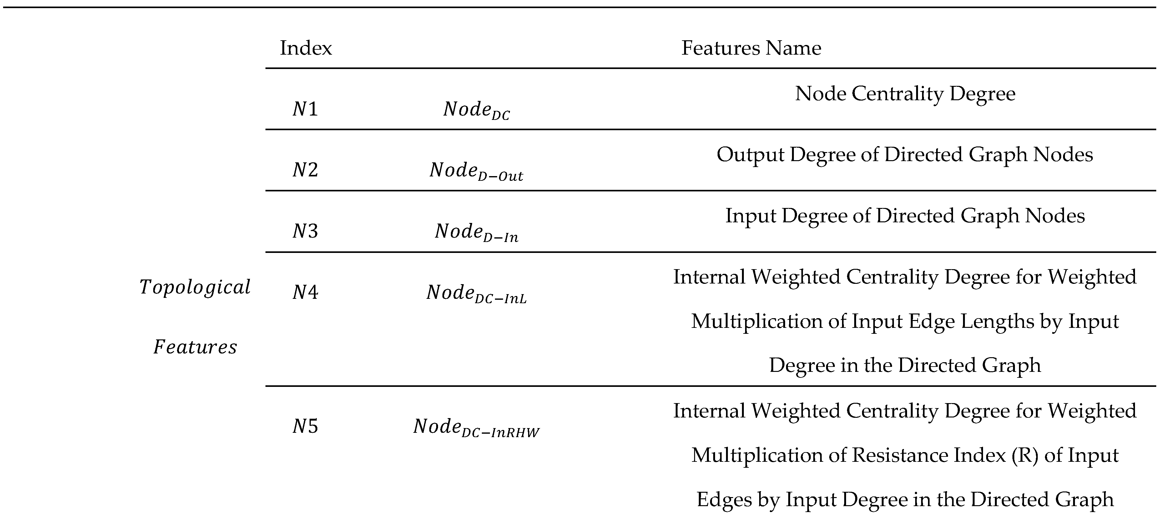
2.3. Topological and Hydraulic Features
The integration of topological and hydraulic features significantly enhances the application of machine learning models in water distribution network (WDN) analysis. Topological features, such as node degree, clustering coefficient, and shortest path, define the network structure and connections, offering valuable insights into its inherent organization and stability. Complementing these are hydraulic features that reflect WDN performance, including average flow velocity in pipes, pressure head at nodes, and flow rates under various conditions.
This study incorporates 80 diverse features as critical input variables for various machine learning algorithms. These features enable supervised machine learning models to learn complex relationships within WDNs, facilitating optimal design without solving hydraulic equations directly. The features used in this research encompass nodes, pipes, and the overall network graph.
Feature assignment follows a specific methodology:
- Node and overall network graph features are assigned to pipes.
- For each pipe, the average of features from connecting nodes is calculated and assigned as a descriptive feature.
- Features derived from the overall network graph are uniformly applied to all pipes within that network, aiding in network differentiation during the learning process.
The study employs both directed and undirected graph representations:
- Undirected graphs are used for features such as square clustering coefficient, node eccentricity, and pipe length index.
- Directed graphs are necessary for features like degree of centrality and shortest path from the reservoir to nodes.
- Some features, including node closeness centrality index and betweenness centrality indices, require examination of both directed and undirected graphs.
Water flow direction determines the graph directionality in WDNs. For features requiring graph weight attributes, either pipe length or the pipe resistance coefficient from the Hazen-Williams equation is used:
where:
- R = Pipe resistance
- = Pipe length
- C = Hazen-Williams coefficient
- = Pipe diameter
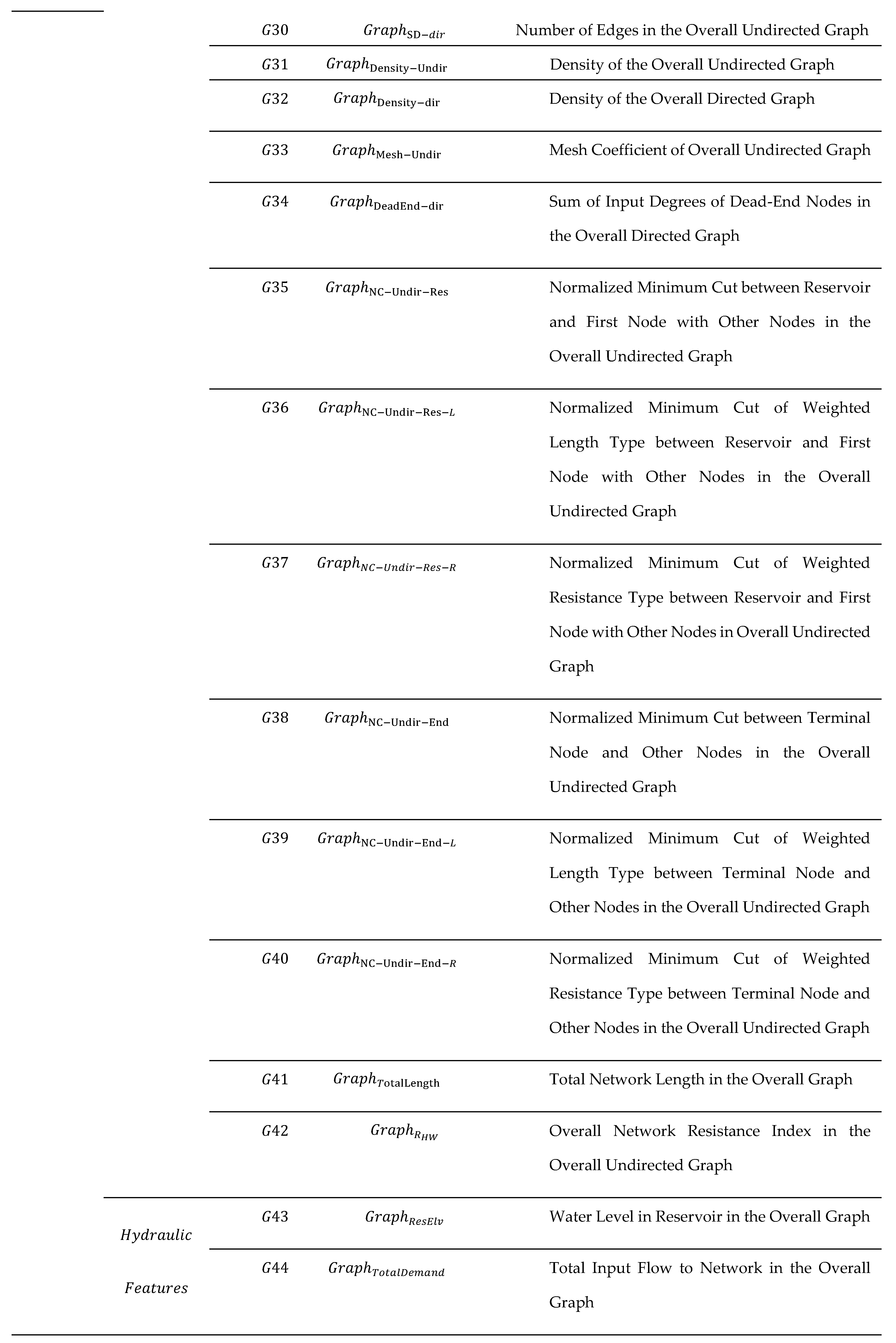
The target feature in this study is the optimal commercial diameters in WDNs, obtained through the optimization process. Table 2 presents a schematic of the features derived from 600 artificial networks. For a comprehensive list of features used in this study, please refer to Table A1 in the article Appendix.
2.4. Database Preparation
The critical stage of database preparation follows the development of the algorithm for randomly generating WDNs and extracting their topological and hydraulic features. This process is essential for creating a suitable dataset for machine learning algorithms and involves two key steps:
- Outlier Data Detection: Identifying and handling outliers is crucial as these anomalous values can significantly impact model training, reducing accuracy and generalizability. In this study outliers are defined as data points that differ by more than four times the standard deviation from the mean of the same data set. Once identified, outliers are removed from the final database.
- Data Normalization: Normalization is performed using the Min-max normalization method. This step is vital for (1) aligning features with different scales, and (2) preventing disproportionate impact of varying value ranges (e.g., pipe lengths vs. node pressures) on machine learning model performance.
By carefully addressing outliers and normalizing the data, we ensure that the machine learning algorithms have a clean, well-prepared dataset to work with, ultimately leading to more reliable and accurate results in WDN analysis and design.
2.5. Feature Selection Methods
Feature selection is a critical step in machine learning model usage, particularly when dealing with datasets containing a large number of features. This process involves identifying and selecting the most relevant and informative features from the original dataset for training a machine learning model. The primary objectives of feature selection are to enhance model performance, mitigate overfitting, accelerate training, and often provide better model interpretability (Zheng and Casari 2018; Venkatesh and Anuradha 2019).
Feature selection methods can be broadly categorized into four groups: Hybrid, Embedded, Wrapper, and Filter, with each method being suitable for feature extraction in different domains (Chandrashekar and Sahin 2014). The present study employs Filter and Embedded categories. Methods such as Var, Kb, and Chi2 fall under the Filter category, while methods like LGB, Per, and Xg belong to the Embedded group.
In Embedded methods, it is essential to tune the hyperparameters of the machine learning model. The selection of the optimal hyperparameter configuration directly impacts model performance (Yang and Shami 2020; Probst et al. 2018). In this study, the Grid search method is used for hyperparameter tuning, which is a theoretical decision-making approach that involves a comprehensive search for a fixed range of hyperparameter values (Injadat et al. 2020).
In the following the detailed explanations of all six feature selection methods used in this study is given.
- 1.
- Chi2
This statistical test is specifically used to examine the dependency between two variables (Liu and Setiono 1995). In feature selection, the chi2 method selects non-negative features that demonstrate the highest statistical dependency on the target variable (Khomytska et al. 2023). In this method, the chi2 value is calculated between each feature and the target variable, with higher chi2 indicating a stronger dependency between the feature and the target. Accordingly, features with larger chi2 values are selected as important features. This method is also well-suited for categorical data, with understanding the concept of variable dependency being relatively straightforward. The main limitation of this method involves its limited applicability to non-negative features and the target variable.
- 2.
- Var
In this simple and fast method, features that show little variation, meaning those with low variance, are removed from dataset (Guyon et al. 2003). The central concept is that features that are almost constant tend not to provide valuable information for the machine-learning model (Fida et al. 2021). A variance threshold is determined to apply this method, with features with variances lower than this value removed from the feature set. Due to its simplicity and high speed, this method is often used as a preprocessing stage for data dimension reduction. However, it should be noted that this method only examines features individually and ignores potential interactions between features. Additionally, selecting an appropriate value for the variance threshold can be somewhat arbitrary and data-dependent.
- 3.
- Kb
This method aims to select the K most relevant features to the target variable (Desyani et al. 2020). For this purpose, univariate statistical tests evaluate the relationship between each feature and the target variable. The functions used in this method assign a score to each feature based on statistical criteria. Subsequently, the K features that have obtained the highest scores are selected as the optimal features. Furthermore, the chi2 test can also be used as a scoring function for non-negative features. This method is relatively fast and efficient and can sufficiently identify features related to the target. However, much like the variance threshold method, Kb method does not account for the interactions between features. It assumes that the relationship of each feature with the target can be independently evaluated.
- 4.
- LGB
LGB is a robust gradient-boosting framework that inherently provides the ability to calculate and deliver feature significance scores (Ye et al. 2019; Hua 2020). This score indicates the impact of each feature on the building of the decision trees in the boosting model. During model training, LGB calculates metrics such as the number of times a feature is used to split nodes in trees, otherwise known as "split," or the reduction in node impurity due to using that feature, otherwise known as "gain." These values are indicators of feature significance. This approach has the advantage of feature selection being directly integrated into the model training process while accounting for the interactions between features. The key hyperparameters of this method, which are tuned before the training process using Grid search, include n_estimators, num_leaves, max_depth, and learning_rate.
- 5.
- Per
This method is applied to evaluate the relative significance of features after training a machine-learning model (Altmann et al., 2010). The model is first employed to predict the significance of any feature. Next, the feature values in the validation set are randomly shuffled. After this alteration, the model’s performance on the altered data is evaluated. A significant drop in performance following the randomization of feature values indicates that the feature is of high significance to the model since the disturbance of its values significantly impacts the model's ability to predict. The advantage of this approach is that it can be used for any trained model, and its conceptual basis is relatively easy to understand. However, it can be computationally costly for large datasets with a high number of features, as it would imply re-evaluating the model performance for every feature. As the model employed in this process is LightGBM, hyperparameters from the previous section are employed.
- 6.
- Xg
Like LGB, Xg is a popular gradient-boosting algorithm that offers feature significance calculation (Hsieh et al. 2019; Alsahaf et al. 2022). Xg, while training the model, assigns feature importance scores in terms of how often a feature is employed for splitting nodes, the split criterion's contribution from the feature-induced split, and the number of samples that are covered by splits of the feature or "coverage." Similar to LGB feature importance, this approach comes with model training inherently and considers interaction among features. It must be noted that the calculated feature significance is specific to the Xg model and may produce different results for other models. The tuned hyperparameters for the current research study are n_estimators, eta, gamma, and max_depth.
2.6. Machine Learning Models
Machine learning is a branch of artificial intelligence that enables computers to learn from data without explicit programming. In other words, instead of providing computers with step-by-step instructions to perform a task, large volumes of data are provided, with specific algorithms being employed to help the computer identify patterns, relationships, and rules within said data and make predictions or decisions based on this knowledge (Riyahi et al. 2018). The primary goal of machine learning is to develop systems that can improve their performance over time with the reception of additional data. This improvement could involve various areas such as prediction accuracy, processing speed, or the ability to recognize more complex patterns.
2.6.1. Regression in Machine Learning
Regression is one of the most critical and widely used aspects of supervised machine learning. Regression problems aim to establish a relationship between input and output variables. In this context, a relationship is developed to predict a continuous objective variable based on one or more predictor variables (Han et al. 2011). In the present study, four machine learning models, namely RF, SVM, BAG, and LGB are used in regression problems, which will be outlined in detail in the following sections.
- 1.
- Random Forest (RF)
The initial idea of the random forest was presented in 1972 by Messenger and Mandell (Messenger and Mandell 1972). This concept was later developed by Cutler et al. (2012). The random forest model is one of the most widely used algorithms in machine learning for classification and regression (Breiman 2001). This model is built on decision trees that are combined to increase prediction accuracy and stability. The main concept here is that each tree is trained independently, and each of said trees makes different decisions regarding the data. The final result is then obtained through voting (for classification problems) or averaging (for regression problems) among the trees. The advantages of random forest include stability and high accuracy. By reducing overfitting and providing diversity in predictions, this model achieves high accuracy in complex problems. Another advantage of the random forest model is its resistance to noise. Specifically, this model is less sensitive to noise and incorrect data due to the utilization of multiple trees. The adjusted hyperparameters of this method in the present study include n_estimators, min_samples_split, and max_depth.
- 2.
- SVM
SVM is one of the powerful and widely used algorithms in supervised machine learning (Cortes and Vapnik 1995). This algorithm is specifically used in classification and regression problems. The main concept behind SVM is locating an optimal hyperplane that separates data in the best possible way. The "optimal hyperplane" denotes locating a hyperplane that maximizes the margin. The margin refers to the distance between the hyperplane and the closest data points from objective function value. These close points are called "support vectors" and play a key role in determining the hyperplane position (Vapnik 2013). In other words, only these points impact the hyperplane location, with other data points having zero impact. SVMhas multiple advantages. This algorithm performs particularly well in high-dimensional spaces and is memory-efficient due to its focus on support vectors. Nevertheless, SVMs are still recognized as valuable tools in the machine learning toolkit due to their high accuracy and decent generalization capabilities. Thus, they are widely used in various fields, including machine vision, natural language processing, and bioinformatics (Scholkopf and Smola 2018; Ben-Hur and Weston 2010). The adjusted hyperparameters of this method in the present study include regularization parameter (C), Kernel, and gamma.
- 3.
- BAG
This idea was first used by Breiman et al. (1996) to predict classification and regression models, where they evaluated different models by varying the number of bags, with the results ultimately showing an increase in accuracy through the use of the combined BAG model (Breiman 1996). The BAG model approach is an ensemble learning process that creates multiple instances of a learner, a classifier in this case, to result in multiple predictions (Gaikwad and Thool 2015). The final model output is obtained using a combination rule (i.e., majority voting) of outputs from each created subspace. The generation of multiple samples is conducted by creating self-initiated iterations from the learning set, where samples are randomly drawn from the entire training data with replacement, placing the same number of samples in each subset (Tuysuzoglu and Birant 2020). The adjusted hyperparameters in this method in the present study include n_estimators, max_samples, and max_features.
- 4.
- LGB
The initial concept of boosting learning methods was presented by Schapire (1990). In this learning model, the goal is to boost performance. The performance of this method involves implementing a weak learner on the data, which is then enhanced to a strong learner in subsequent stages (Ke et al. 2017). The boosting learning method consists of various types, including the Gradient Boosting model, which transforms a weak learner into a strong learner. The LGB model is an optimized version of the Gradient Boosting framework designed for efficient regression and classification, particularly for high-dimensional data.
The risk of overfitting increased in previous models with increased tree depth, given the Level-Wise logic, which incrementally increased tree depth during training to improve model accuracy. However, in the new logic of the LGB algorithm, the enhancement and training process is Leaf-Wise, meaning that the best branching between leaves (features) is selected in each stage of the decision tree. This process is quite effective in increasing computational speed and reducing overfitting risk. The fundamental hyperparameters of this method were previously described in earlier sections.
2.6.2. Model Evaluation
Two criteria, and RMSE, are used to evaluate machine learning models. These criteria demonstrate the effectiveness and suitability of machine learning models for the dataset. The criterion indicates how much of the variance in the objective variable is explained by the model (Kutner et al. 2004). Furthermore, the RMSE criterion shows how far the predicted values are from the actual values. The relationships between these two criteria are as follows:
The values , , , and are outlined below:
- : The real value of the objective variable.
- : The predicted value of objective variable.
- : The mean value of objective variable.
- : The total number of samples.
2.6.3. Hanoi WDN
The most effective machine learning model, as determined by the comparative analysis, is selected for application to the Hanoi Water Distribution Network (WDN). Originally introduced by Fujiwara and Khang in 1990, the Hanoi WDN serves as a benchmark case study in water distribution system optimization. This network consists of 32 nodes, 34 pipes, 3 loops and1 reservoir with a water elevation of 100 meters.
Key hydraulic parameters of the Hanoi WDN include:
- Minimum pressure head at demand nodes: 30 meters
- Hazen-Williams coefficient for all pipes: 130
Figure 2 provides a visual representation of the Hanoi WDN layout, illustrating the network's topological structure and component relationships.
Figure 2 presents the demand at each node. Additionally, the pipe lengths in order of their respective numbers are: {100, 1350, 900, 1150, 1450, 450, 850, 850, 800, 950, 1200, 3500, 800, 500, 550, 2730, 1750, 800, 400, 2200, 1500, 500, 2650, 1230, 1300, 850, 300, 750, 1500, 2000, 1600, 150, 860, 950}. Five commercial pipe diameters are utilized in the design of the Hanoi WDN: 12, 16, 20, 24, 30, and 40 inches.
3. Results and Discussion
The first stage in the developed model involves the generation of synthetic WDNs. This process utilizes a developed algorithm that includes the graph mining library in Python (NetworkX), the EPANET Toolkit in Python (EPyT), and the genetic algorithm optimizer (geneticalgorithm2). Figure 3 shows the output of three synthetic WDNs. As evident from these WDNs, all components of the generated networks are interconnected, with no pipes interfering with each other. The minimum and maximum number of pipes connected to each node are 1 and 4, respectively. Finally, appropriate random values are assigned to each component of the generated networks to enable the hydraulic design process. For instance, as previously mentioned, pipe lengths are assigned values between 20 and 100 m, or the Hazen-Williams coefficient in pipes is assigned values between 80 and 130. Following the generation of 600 synthetic networks, the design process for the optimal WDN diameters begins. The number of genetic algorithm iterations is 400 iterations on average. Additionally, population size, mutation probability, and crossover probability are set to 12 times the WDN pipes, 0.06, and 0.85, respectively.
The topological and hydraulic features are extracted from the WDNs during the next stage. These features generally concern the topological and hydraulic properties of nodes, pipes, and the overall network graph, totaling 80 characteristics, with the target feature being the optimal pipe diameters. The features obtained for nodes are assigned to the pipes connected to them. This assignment is conducted by calculating the arithmetic mean of the features of the nodes at both sides of each pipe and assigning it as the corresponding pipe feature. Regarding the features obtained for the overall network graph, each extracted feature is assigned to all pipes in that WDN. For instance, the network efficiency feature (G7) illustrated in Table 3 is repeated for all pipes in the WDN with the same G7 value. The features extracted at this stage are presented in Table 3. The dataset, which comprises 80 features for 600 synthetic WDNs, has been uploaded to the GitHub site (https://github.com/bahrami-i/WDNs-Dataset), where readers can conveniently download it for use in their research.
The features depicted in Table 3 correspond to 600 synthetic WDNs, with the number of rows equal to 85,745 samples, the same as the number of pipes in 600 artificial networks. There are 80 columns corresponding to the number of features. Following obtaining topographical and hydraulic features, outliers are identified and removed from the dataset. To this end, all characteristics are examined, and the values exceeding 4 times the standard deviation relative to the data mean according to the Z-Score criterion are identified. The rows containing said features are removed from the dataset. Following the outlier removal process, the number of rows in the dataset decreases from 85,745 to 67,226 rows. Figure 4 compares the frequency histogram of the N4 feature before and after outlier removal. As illustrated, removing outliers has led to variations within the range of the N4 feature.
The dataset is then normalized using the min-max normalization method to scale the features within the 0 to 1 range. This data normalization improves machine learning model performance, increases convergence speed in gradient-based algorithms, and prevents characteristics with larger scales from dominating. Table 4 presents the output of Table 3 features following outlier removal and data normalization.
A visual comparison of Table 3 and Table 4 reveals that the row corresponding to index 85,742 in Table 3 has been removed from Table 4, which as previously explained, occurred due to outlier removal. Additionally, it is clear from Table 4 that the data have been normalized between 0 and 1 after data normalization process. The dataset is divided into training and test data sets during the next stage. Seventy percent of the total data is assigned to training data, while thirty percent is designated for test data.
The next stage involves performing essential feature extraction from the 80 existing features in the dataset. To this end, as previously stated, six models, namely Var, Kb, Chi2, LGB, Per, and Xg, are utilized. The Var, Chi2, and Kb models belong to the Filter model category, while the LGB, Xg, and Per models belong to the Embedded category. The hyperparameter tuning in Embedded models is carried out using the Grid search algorithm. Table 5 depicts the hyperparameter values of the Embedded models tuned using the Grid search algorithm. Additionally, Table 6 illustrates the top 20 features provided by the feature selection methods.
The analysis of results feature selection methods in Table 6 reveals several key insights:
Feature importance by category:
- Node-related features dominate in four methods (Xg, Per, LGB, and Chi2)
- Overall network graph properties are most prominent in two methods (Kb and Var)
Significance of specific features:
- N5 and N7 (weighted node centrality degrees) consistently appear in the top quartile for most methods, except Var
- Features using pipe resistance (R) as a weighted criterion show greater importance than those using pipe length
Distribution of top features:
- Node features: 50% on average
- Pipe features: 26% on average
- Graph features: 24% on average
Method-specific observations:
- Filter methods (e.g., Kb and Var) tend to select more overall network graph features
- Embedded methods (e.g., Xg, Per, LGB) primarily select node and pipe features
Application to machine learning:
- Top features from each selection method are paired with corresponding optimal diameters
- These feature sets are used as inputs for four machine learning models
- Hyperparameters for each model are optimized using the Grid search algorithm (detailed in Table 7)
Thus, 24 combined machine learning models are trained and ultimately evaluated with test data. The evaluation metrics used are and RMSE. Figure 5 shows the output of 24 coupled machine learning models. As observed in this figure, the strongest model based on both evaluation metrics is the Xg-LGB model, which implements the best features of the Xg method on the LGB regressor, with and RMSE values at 0.98 and 0.02, respectively. The weakest model is Var-SVM, with and RMSE values at 0.41 and 0.21, respectively.
After selecting the best machine learning method, the Xg-LGB model, this model is used to find the optimal diameters in the Hanoi WDN. The results show that is 0.94, indicating a high percentage of variance in the objective values (optimal diameters presented by Kadu et al. 2008) identified by the Xg-LGB model. Furthermore, the RMSE value is 0.06, indicating that a small percentage of variance in the objective values remains unidentified by the model due to various factors: a shortage of features, measurement errors, incidental noise, model limitations, and data limitations. By improving each of the mentioned factors, the model's efficiency could be enhanced. Table 8 presents the diameters calculated by the Xg-LGB model for the Hanoi WDN, along with the diameters of this network presented by Kadu. From the table, the diameters obtained by the Xg-LGB model are continuous values and rounded to the nearest commercial diameter. By comparing these diameters with Kadu's findings, it becomes clear that in approximately 65% of cases, the forecasted diameters of the Xg-LGB model are equal to Kadu's outputs, while in the remaining 35%, these diameters are one size larger than Kadu's results. Since Kadu's findings are obtained by applying the genetic optimization algorithm, the high level of consistency in the results predicted by the Xg-LGB model can be reasoned as follows: first, the original synthetic database presented in Table 3 is suitable for generating the optimal diameters for a given number of random WDNs; second, the Xg feature selection method in Table 6 has effectively identified the efficient features corresponding to the objective function; and third, the Xg-LGB model has well been trained concerning the original synthetic database and then to the Hanoi benchmark network, all of which can somehow embody the appropriate generalization of the model.
Additionally, using the predicted diameter results from the Xg-LGB model on the Hanoi WDN and conducting the hydraulic simulation with Epanet software, the nodal pressure heads are obtained, displayed in the last column of Table 8. Except for node 2, which has a pressure of 97.14 meters (due to its proximity to the reservoir), the pressures at other nodes range from 35 to 65 meters. This improves the minimum pressure derived from Kadu's diameter results and meets the maximum pressure requirements, which are essential for ensuring adequate pressure in consumer nodes.
4. Conclusion
The optimal design of WDNs is one of the most critical engineering challenges, directly impacting service quality, economic costs, and water resource sustainability. Given urban population growth and increasing water demand, there is an increasingly urgent need for efficient methods to design these networks. Traditional WDN design methods are often time-consuming and have significant limitations when facing complex networks. Thus, developing novel and intelligent methods that can perform optimal design with high speed and accuracy seems essential.
A novel machine learning-based approach for optimal water distribution network design was presented in this study. To this end, 600 synthetic WDNs were generated and optimized. Then, 80 topological and hydraulic features concerning nodes, pipes, and the overall network graph were extracted from the optimized WDNs. Following data preprocessing, including outlier detection and normalization, six feature selection methods, namely Chi2, Var, Kb, LGB, Permutation, and Xg, were employed. Subsequently, four machine learning algorithms, including RF, SVM, LGB, and BAG, were utilized in combination with feature selection methods. Results showed that the LGB-Xg method had the best performance based on and RMSE in optimal WDN design. This combination method not only demonstrated higher accuracy compared to other methods but also showed significant capability in generalizability and predicting optimal pipe diameters. Finally, the LGB-Xg method is applied to a real-world WDN, the Hanoi WDN, demonstrating that this model can predict the optimal pipe diameters with R² and RMSE values of 0.94 and 0.06, respectively. The research results indicated that among node, pipe, and overall network graph features, topological and hydraulic node features are of very high importance. This study demonstrates that using machine learning approaches can significantly improve water WDN design processes. Moreover, the study results can serve as a guideline for engineers and designers in the selection of appropriate pipe diameters in WDNs.
It is recommended that future studies investigate and explore the feasibility of using graph neural networks as an alternative to coupled machine learning models. Additionally, other factors such as reliability and uncertainty could be considered when developing machine learning methods for designing WDNs that achieve optimal diameters and enhance reliability.
Acknowledgments
This project is partially funded by the Deutsche Forschungsgemeinschaft (DFG) under Project number 544048327.
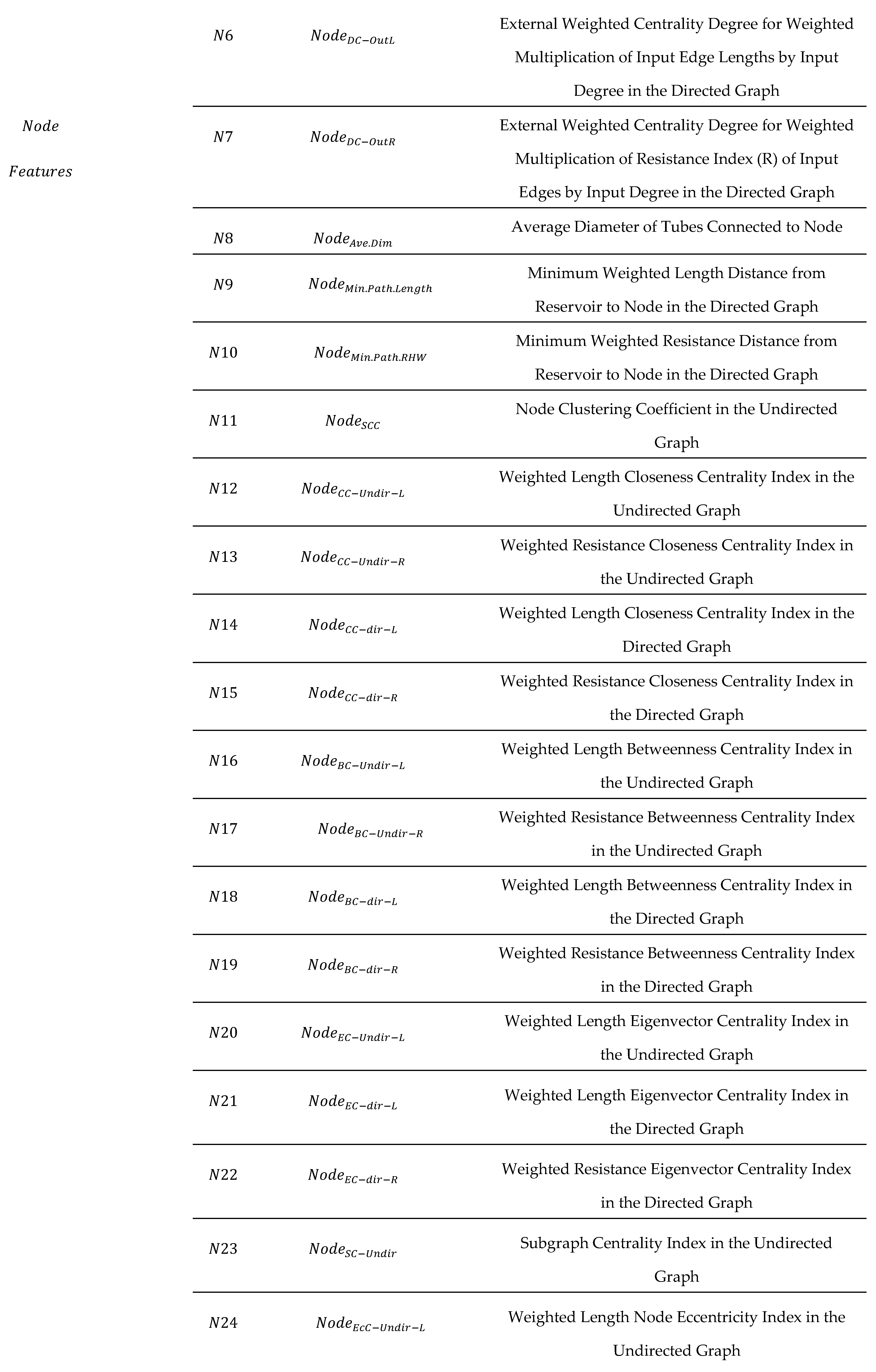
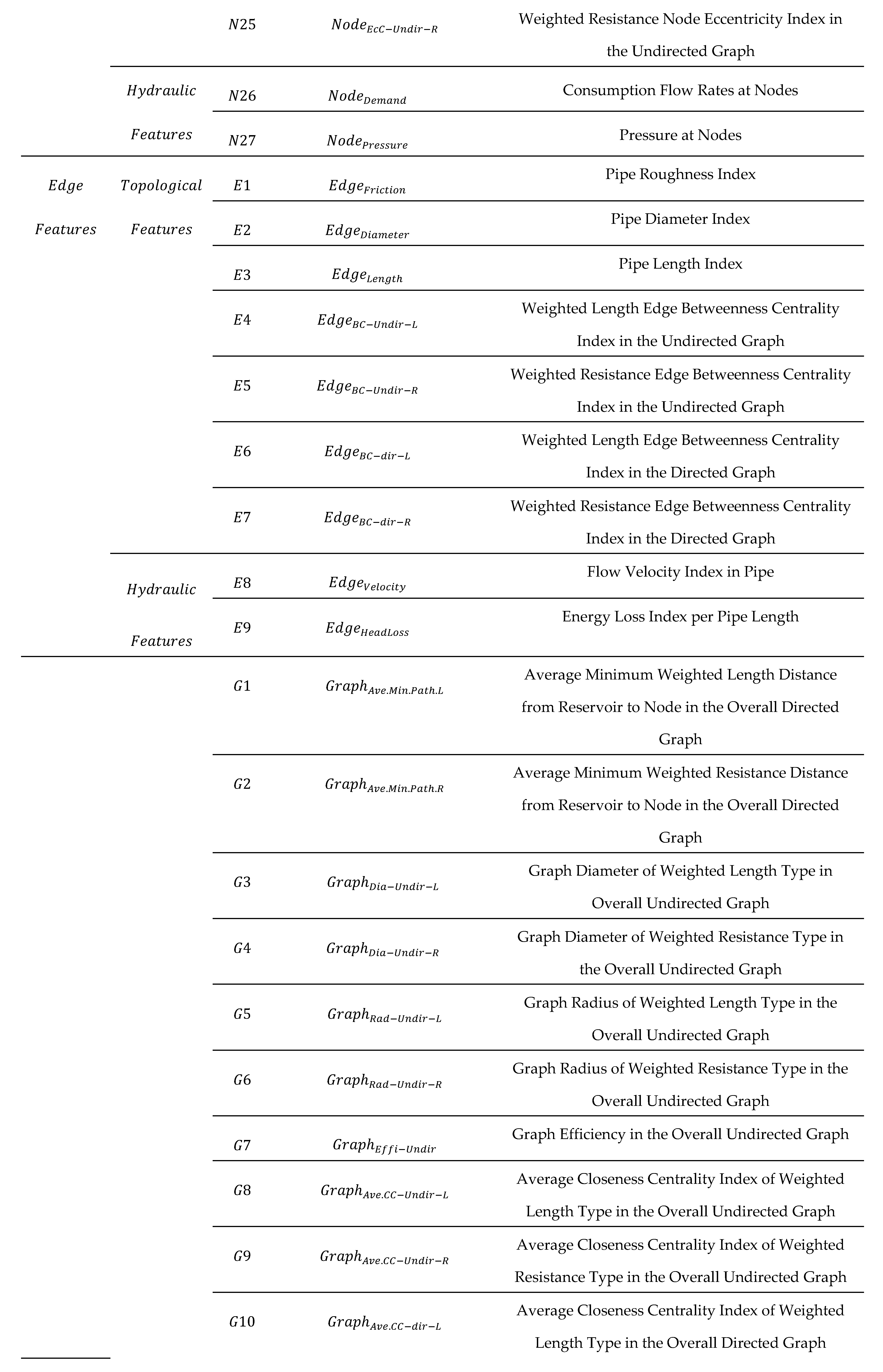
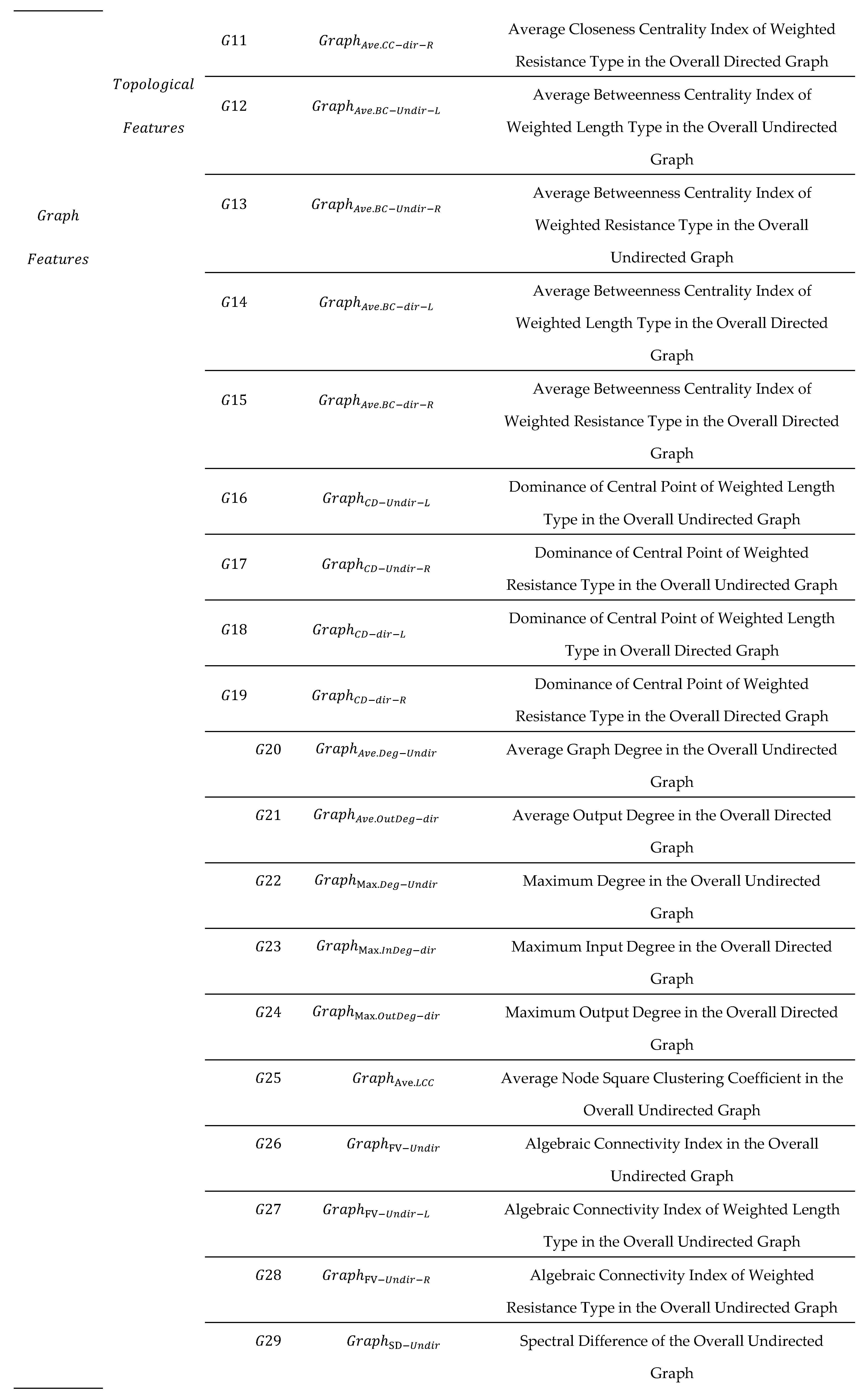
Appendix A

Table A1.
Complete List of Features Used in this Study.
References
- Ahmed, A. A.; Sayed, S.; Abdoulhalik, A.; Moutari, S.; Oyedele, L. Applications of machine learning to water resources management: A review of present status and future opportunities. Journal of Cleaner Production 2024, 140715. [Google Scholar] [CrossRef]
- Alsahaf, A.; Petkov, N.; Shenoy, V.; Azzopardi, G. A framework for feature selection through boosting. Expert Systems with Applications 2022, 187, 115895. [Google Scholar] [CrossRef]
- Altmann, A.; Toloşi, L.; Sander, O.; Lengauer, T. Permutation importance: a corrected feature importance measure. Bioinformatics 2010, 26, 1340–1347. [Google Scholar] [CrossRef]
- Amali, S.; Faddouli, N.E.E.; Boutoulout, A. Machine learning and graph theory to optimize drinking water. Procedia Computer Science 2018, 127, 310–319. [Google Scholar] [CrossRef]
- Arsene, C.T.; Gabrys, B.; Al-Dabass, D. Decision support system for water distribution systems based on neural networks and graphs theory for leakage detection. Expert Systems with Applications 2012, 39, 13214–13224. [Google Scholar] [CrossRef]
- Ben-Hur, A.; Weston, J. A user’s guide to support vector machines. Data mining techniques for the life sciences 2010, 223–239. [Google Scholar] [CrossRef]
- Bondy, J.A.; Murty, U. S. R 1976. GRAPH THEORY WITH APPLICATIONS. Elsevier Science Publishing Co.; Inc. 52 Vanderbilt Avenue, New York, N.Y. 10017.
- Breiman, L. Bagging Predictors. Machine Learning 1996, 123–140. [Google Scholar] [CrossRef]
- Breiman, L. Random Forest. Machine Learning 2001, 45, 5–32. [Google Scholar] [CrossRef]
- Chandrashekar, G.; Sahin, F. A survey on feature selection methods. Computers & electrical engineering 2014, 40, 16–28. [Google Scholar] [CrossRef]
- Chawla, N.V.; Bowyer, K.W.; Hall, L.O.; Kegelmeyer, W.P. SMOTE: synthetic minority over-sampling technique. Journal of artificial intelligence research 2002, 16, 321–357. [Google Scholar] [CrossRef]
- Chen, T.Y.J.; Guikema, S.D. Prediction of water main failures with the spatial clustering of breaks. Reliability Engineering & System Safety 2020, 203, 107108. [Google Scholar] [CrossRef]
- Cheng, M.; Li, J. Optimal sensor placement for leak location in water distribution networks: A feature selection method combined with graph signal processing. Water research, 2023, 242, 120313. [Google Scholar] [CrossRef]
- Coelho, M.; Austin, M.A.; Mishra, S.; Blackburn, M. Teaching Machines to Understand Urban Networks: A Graph Autoencoder Approach. International Journal on Advances in Networks and Services 2020, 13, 70–81. Available online: https://www.researchgate.net/publication/348992449.
- Cortes, C.; Vapnik, V. Support-vector networks. Mach Learn. 1995, 20, 273–297. [Google Scholar] [CrossRef]
- Creaco, E.; Franchini, M. Low Level Hybrid Procedure for the Multi-Objective Design of Water Distribution Networks. Procedia Engineering 2014, 70, 369–378. [Google Scholar] [CrossRef]
- Cutler, A.; Cutler, D.R.; Stevens, J.R. Random forests. Ensemble machine learning: Methods and applications 2012, 157–175. [Google Scholar] [CrossRef]
- Desyani, T.; Saifudin, A.; Yulianti, Y. Feature selection based on naive bayes for caesarean section prediction. IOP Conference Series: Materials Science and Engineering 2020, 879, 012091. [Google Scholar] [CrossRef]
- Deuerlein, J. W. Decomposition model of a general water supply network graph. Journal of Hydraulic Engineering 2008, 134, 822–832. [Google Scholar] [CrossRef]
- Di Nardo, A.; Di Natale, M.; Giudicianni, C.; Musmarra, D.; Santonastaso, G.F.; Simone, A. Water distribution system clustering and partitioning based on social network algorithms. Procedia Engineering 2015, 119, 196–205. [Google Scholar] [CrossRef]
- Di Nardo, A.; Giudicianni, C.; Greco, R.; Herrera, M.; Santonastaso, G.F. Applications of graph spectral techniques to water distribution network management. Water 2018, 10, 1–16. [Google Scholar] [CrossRef]
- Duan, N.; Mays, L. W.; Lansey, K. E. Optimal Reliability-Based Design of Pumping and Distribution Systems. Journal of Hydraulic Engineering 1990, 116, 249–268. [Google Scholar] [CrossRef]
- Farmani, R.; Walters, G. A.; Savic, D. A. Trade-Off Between Total Cost and Reliability for Anytown Water Distribution Network. Journal of Water Resources Planning and Management 2005, 131, 161–171. [Google Scholar] [CrossRef]
- Farmani, R.; Walters, G.; Savic, D. Evolutionary Multi-Objective Optimization of the Design and Operation of Water Distribution Network: Total Cost Vs. Reliability Vs. Water Quality. Journal of Hydroinformatics 2006, 8, 165–179. [Google Scholar] [CrossRef]
- Fida, M.A.F.A.; Ahmad, T.; Ntahobari, M. October. Variance threshold as early screening to Boruta feature selection for intrusion detection system. 2021 13th International Conference on Information & Communication Technology and System (ICTS); 2021; pp. 46–50. [Google Scholar] [CrossRef]
- Fujiwara, O.; Khang, D.B. A two-phase decomposition method for optimal design of looped water distribution networks. Water Resour Res 1990, 26, 539–549. [Google Scholar] [CrossRef]
- Gaikwad, D.P.; Thool, R.C. February. Intrusion detection system using bagging ensemble method of machine learning. 2015 international conference on computing communication control and automation; 2015; pp. 291–295. [Google Scholar] [CrossRef]
- Giudicianni, C.; Nardo, A.; Oliva, G.; Scala, A.; Herrera, M. A Dimensionality-Reduction Strategy to Compute Shortest Paths in Urban Water Networks. arXiv 2019. [Google Scholar] [CrossRef]
- Grammatopoulou, M.; Kanellopoulos, A.; Vamvoudakis, K.G.; Lau, N. A Multi-step and Resilient Predictive Q-learning Algorithm for IoT with Human Operators in the Loop: A Case Study in Water Supply Networks. arXiv 2020, arXiv:2006.03899. [Google Scholar] [CrossRef]
- Gupta, I. Linear Programming Analysis of a Water Supply System. AIIE Transactions 1969, 1, 56–61. [Google Scholar] [CrossRef]
- Guyon, I.; Elisseeff, A. An introduction to variable and feature selection. Journal of machine learning research 2003, 3, 1157–1182. [Google Scholar]
- Hamam, Y.M.; Brameller, A. Hybrid method for the solution of piping networks. Proc. of the IEEE 1971, 118, 1607–1612. [Google Scholar] [CrossRef]
- Han, J.; Pei, J.; Kamber, M. Data mining: Concepts and techniques; Elsevier, 2011. [Google Scholar]
- Han, R.; Liu, J.; Spectral clustering and genetic algorithm for design of district metered areas in water distribution systems. Procedia Engineering 2017, 186, 152–159. https://doi.org/10.1016/j.proeng.2017.03.221. Hsieh, C.P.; Chen, Y.T.; Beh, W.K.; Wu, A.Y.A 2019, October. Feature selection framework for XGBoost based on electrodermal activity in stress detection. In 2019 IEEE International Workshop on Signal Processing Systems (SiPS).; 330-335. IEEE. http://dx.doi.org/10.1109/SiPS47522.2019.9020321.
- Hua, Y. An efficient traffic classification scheme using embedded feature selection and lightgbm. 2020 Information Communication Technologies Conference (ICTC); 2020; pp. 125–130. [Google Scholar] [CrossRef]
- Injadat, M. N.; Moubayed, A.; Nassif, A.B.; Shami, A. Systematic Ensemble Model Selection Approach for Educational Data Mining. Knowledge-Based Systems 2020, 200. [Google Scholar] [CrossRef]
- Jung, D.; Yoo, D.; Kang, D.; Kim, J. Linear model for estimating water distribution system reliability. Journal of Water Resources Planning and Management. ASCE 2016, 142. [Google Scholar] [CrossRef]
- Kadu, MS.; Gupta, R.; Bhave, PR. Optimal design of water networks using a modified genetic algorithm with reduction in search space. J Water Resour Plan Manage 2008, 134, 147–160. [Google Scholar] [CrossRef]
- Kang, J.; Park, Y.J.; Lee, J.; Wang, S.H.; Eom, D.S. Novel leakage detection by ensemble CNN-SVM and graph-based localization in water distribution systems. IEEE Transactions on Industrial Electronics 2017, 65, 4279–4289. [Google Scholar] [CrossRef]
- Karmeli, D.; Gadish, Y.; Meyers, S. Design of Optimal Water Distribution Networks. Journal of the Pipeline Division 1968, 94, 1–10. [Google Scholar] [CrossRef]
- Ke, G.; Meng, Q.; Finley, T.; Wang, T.; Chen, W.; Ma, W.; Ye, Q.; Liu, T.Y. Lightgbm: A highly efficient gradient boosting decision tree. Advances in neural information processing systems 2017, 30. [Google Scholar]
- Kesavan, H.K.; Chandrashekar, M. Graph theoretic models for pipe network analysis. J. Hydraul. Div 1972, 98, 345–364. [Google Scholar] [CrossRef]
- Khomytska, I.; Bazylevych, I.; Teslyuk, V.; Karamysheva, I. The chi-square test and data clustering combined for author identification. 2023 IEEE 18th International Conference on Computer Science and Information Technologies (CSIT); 2023; pp. 1–5. [Google Scholar] [CrossRef]
- Kutner, M. H.; Nachtsheim, C. J.; Neter, J. Applied Linear Statistical Models, 5th ed.; McGraw-Hill/Irwin, 2004. [Google Scholar]
- Kyriakou, M.S.; Demetriades, M.; Vrachimis, S.G.; Eliades, D.G.; Polycarpou, M.M. EPyT: An EPANET-Python Toolkit for Smart Water Network Simulations. Journal of Open Source Software 2023, 8(92), 5947. [Google Scholar] [CrossRef]
- Liu, H.; Setiono, R. Chi2: Feature selection and discretization of numeric attributes. Proceedings of 7th IEEE international conference on tools with artificial intelligence; 1995; pp. 388–391. [Google Scholar] [CrossRef]
- Liy-González, P.-A.; Santos-Ruiz, I.; Delgado-Aguiñaga, J.-A.; Navarro-Díaz, A.; López-Estrada, F.-R.; Gómez-Peñate, S. Pressure interpolation in water distribution networks by using Gaussian processes: Application to leak diagnosis. MDPI Water 2024, 12, 1147. [Google Scholar] [CrossRef]
- Makaremi, Y.; Haghighi, A.; Ghafouri, H. R. Optimization of Pump Scheduling Program in Water Supply Systems Using a Self-Adaptive NSGA-II; a Review of Theory to Real Application. Water Resour Manage 2017, 31, 1283–1304. [Google Scholar] [CrossRef]
- Murphy, L. J.; Simpson, A. R. Pipe Optimisation Using Genetic Algorithms. Research Report No. R93. Department of Civil Engineering, University of Adelaide. 1992. [Google Scholar]
- Ostfeld, A. Water distribution systems connectivity analysis. Journal of Water Resources Planning and Management 2005, 131, 58–66. [Google Scholar] [CrossRef]
- Prasad, T. D.; Park, N. S. Multiobjective Genetic Algorithms for Design of Water Distribution Networks. Journal of Water Resources Planning and Management 2004, 130, 73–82. [Google Scholar] [CrossRef]
- Price, E.; Ostfeld, A. Graph theory modeling approach for optimal operation of water distribution systems. Journal of Hydraulic Engineering 2016, 142, 04015061. [Google Scholar] [CrossRef]
- Price, E.; Ostfeld, A. Optimal pump scheduling in water distribution systems using graph theory under hydraulic and chlorine constraints. J. Water Resour. Plan. Manag. 2016, 142, 04016037. [Google Scholar] [CrossRef]
- Probst, P.; Boulesteix, A.-L.; Bischl, B. Tunability: Importance of Hyperparameters of Machine Learning Algorithms. Journal of Machine Learning Research 2018, 1–32. [Google Scholar] [CrossRef]
- Rajeswaran, A.; Narasimhan, S.; Narasimhan, S. Graph Partitioning Algorithm for Leak Detection in Water Distribution Networks. J.Computers and Chemical Engineering 2018, 108, 11–23. [Google Scholar] [CrossRef]
- Riyahi, M.M.; Rahmanshahi, M.; Ranginkaman, M.H. Frequency domain analysis of transient flow in pipelines; application of the genetic programming to reduce the linearization errors. Journal of Hydraulic Structures 2018, 4, 75–90. [Google Scholar] [CrossRef]
- Riyahi, M. M.; Bakhshipour, A. E.; Haghighi, A. Probabilistic Warm Solutions-Based Multi-Objective Optimization Algorithm, Application in Optimal Design of Water Distribution Networks. Sustainable Cities and Society 2023, 91, 104424. [Google Scholar] [CrossRef]
- Riyahi, M.M.; Bakhshipour, A.E.; Giudicianni, C.; Dittmer, U.; Haghighi, A.; Creaco, E. An Analytical Solution for the Hydraulics of Looped Pipe Networks. Engineering Proceedings 2024, 69, 4. [Google Scholar] [CrossRef]
- Riyahi, M.M.; Giudicianni, C.; Haghighi, A.; Creaco, E. Coupled multi-objective optimization of water distribution network design and partitioning: a spectral graph-theory approach. Urban Water Journal 2024, 1–12. [Google Scholar] [CrossRef]
- Robert Messenger, R.; and Lewis Mandell, L. A Modal Search Technique for Predictibe Nominal Scale Multivariate Analys. Journal of the American Statistical Association 1972, 768–772. [Google Scholar] [CrossRef]
- Rossman, L.A.; Woo, H.; Tryby, M.; Shang, F.; Janke, R.; Haxton, T. EPANET 2.2 User Manual; Water Infrastructure Division. Center for Environmental Solutions and Emergency Response, 2020. [Google Scholar]
- Samani, H. M.; Taghi, S. Optimization of Water Distribution Networks. Journal of Hydraulic Research 1996, 34, 623–632. [Google Scholar] [CrossRef]
- Savic, D. A.; Walters, G., A. Genetic Algorithms for Least-Cost Design of Water Distribution Networks. Journal of Water Resources Planning and Management 1997, 123, 67–77. [Google Scholar] [CrossRef]
- Schaake, J. C., Jr; Lai, D. Linear Programming and Dynamic Programming Application to Water Distribution Network Design. Massachusetts Institute of Technology. Department of Civil Engineering: M.I.T. Hydrodynamics Laboratory 1969. [Google Scholar]
- Schapire, R.E. The strength of weak learnability. Machine Learning 1990, 5, 197–227. [Google Scholar] [CrossRef]
- Scholkopf, B.; Smola, A.J. Learning with kernels: support vector machines, regularization, optimization, and beyond; MIT press, 2018. [Google Scholar]
- Simpson, A. R.; Dandy, G. C.; Murphy, L. J. Genetic Algorithms Compared to Other Techniques for Pipe Optimization. Journal of Water Resources Planning and Management 1994, 120, 423–443. [Google Scholar] [CrossRef]
- Su, Y. C.; Mays, L. W.; Duan, N.; Lansey, K. E. Reliability-Based Optimization Model for Water Distribution Systems. Journal of Hydraulic Engineering 1987, 113, 1539–1556. [Google Scholar] [CrossRef]
- Swamee, P.K.; Sharma, A.K. Design of Water Supply Pipe Networks; John Wiley: New Jersey, 2008. [Google Scholar] [CrossRef]
- Todini, E. Looped Water Distribution Networks Design Using a Resilience Index Based Heuristic Approach. Urban Water 2000, 2, 115–122. [Google Scholar] [CrossRef]
- Tuysuzoglu, G.; Birant, D. Enhanced Bagging (eBagging): A Novel Approach for Ensemble Learning. The International Arab Journal of Information Technology 2020, 17, 515–528. [Google Scholar] [CrossRef]
- Tzatchkov, V.G.; Alcocer-Yamanaka, V.H.; Bourguett Ortíz, V. Graph Theory Based Algorithms for Water Distribution Network Sectorization Projects. In Water Distribution Systems Analysis Symposium; American Society of Civil Engineers: Cincinnati, OH, USA, 2016; pp. 1–15. [Google Scholar] [CrossRef]
- Ulanicki, B.; Zehnpfund, A.; Martinez, F. Simplification of water distribution network models. in Proc.; 2nd Int. Conf. on Hydroinformatics. Balkema Rotterdam, Netherlands.;, 493–500. 1996. [CrossRef]
- Ulusoy, A.-J.; Stoianov, I.; Chazerain, A. Hydraulically informed graph theoretic measure of link criticality for the resilience analysis of water distribution networks. Applied network science 2018, 3. [Google Scholar] [CrossRef]
- Vapnik, V. The nature of statistical learning theory. Springer science & business media. 2013. [Google Scholar]
- Venkatesh, B.; Anuradha, J. A review of feature selection and its methods. Cybernetics and information technologies 2019, 19, 3–26. [Google Scholar] [CrossRef]
- Xia, W.; Wang, S.; Shi, M.; Xia, Q.; Jin, W. Research on partition strategy of an urban water supply network based on optimized hierarchical clustering algorithm. Water Supply 2022, 22, 4387–4399. [Google Scholar] [CrossRef]
- Yang, L.; Shami, A. On Hyperparameter Optimization of Machine Learning Algorithms: Theory and Practice. Neurocomputing 2020, 415, 1–69. [Google Scholar] [CrossRef]
- Yazdani, A.; Jeffrey, P. Robustness and vulnerability analysis of water distribution networks using graph theoretic and complex network principles. Water Distribution Systems Analysis 2010, 933–945. [Google Scholar] [CrossRef]
- Yazdani, A.; Otoo, R.A.; Jeffrey, P. Resilience enhancing expansion strategies for water distribution systems: A network theory approach. Environmental Modelling and Software 2011, 26, 1574–1582. [Google Scholar] [CrossRef]
- Ye, Y.; Liu, C.; Zemiti, N.; Yang, C. Optimal feature selection for EMG-based finger force estimation using LightGBM model. 2019 28th IEEE international conference on robot and human interactive communication (RO-MAN); 2019; pp. 1–7. [Google Scholar] [CrossRef]
- Zheng, A.; Casari, A. Feature engineering for machine learning: Principles and Techniques for Data Scientists; O'Reilly Media, Inc., 2018. [Google Scholar]
Figure 1.
Flowchart of the developed machine learning model based on graph theory for water distribution network design.
Figure 1.
Flowchart of the developed machine learning model based on graph theory for water distribution network design.
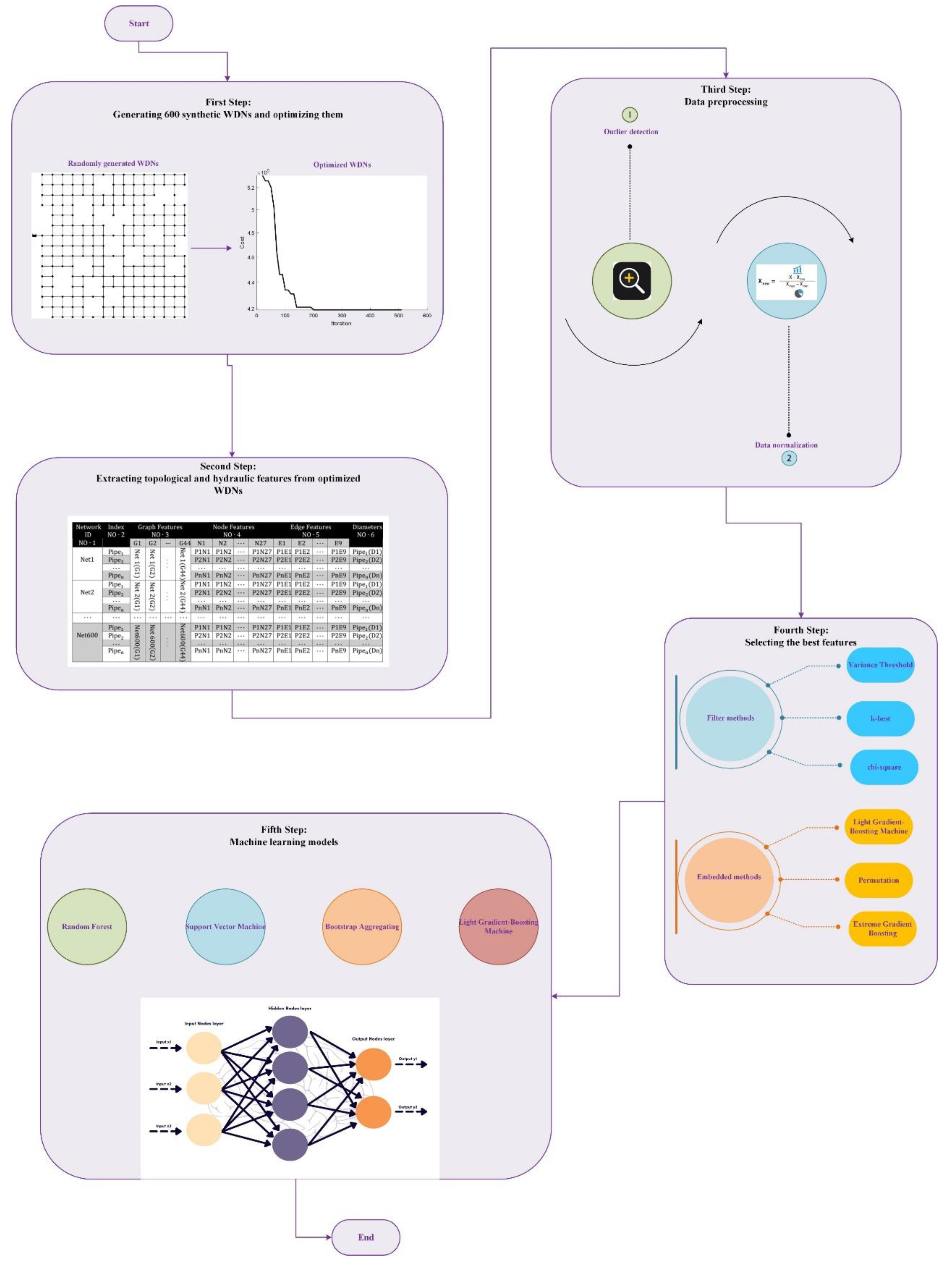
Figure 2.
Hanoi WDN.
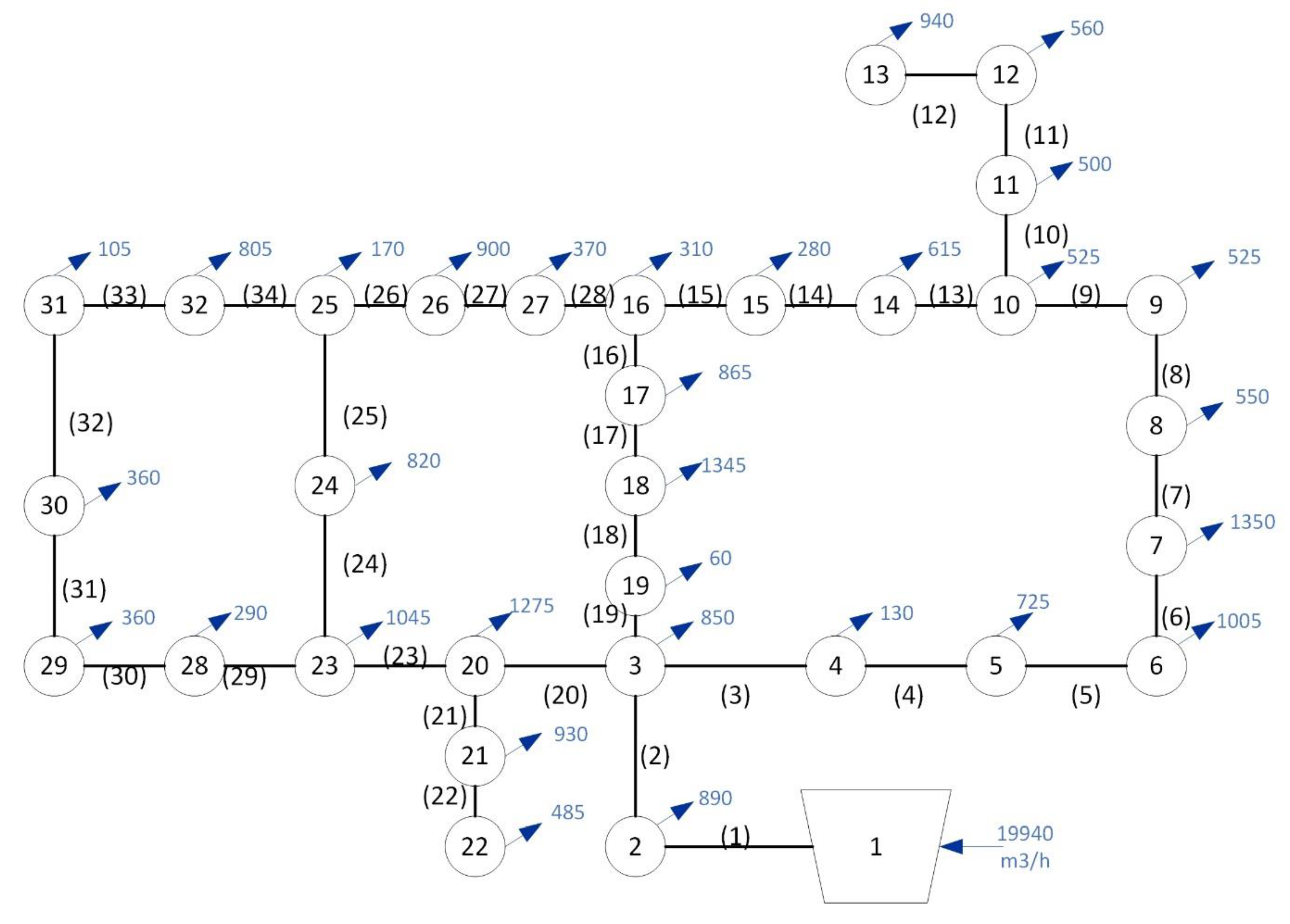
Figure 3.
Generated synthetic WDNs.
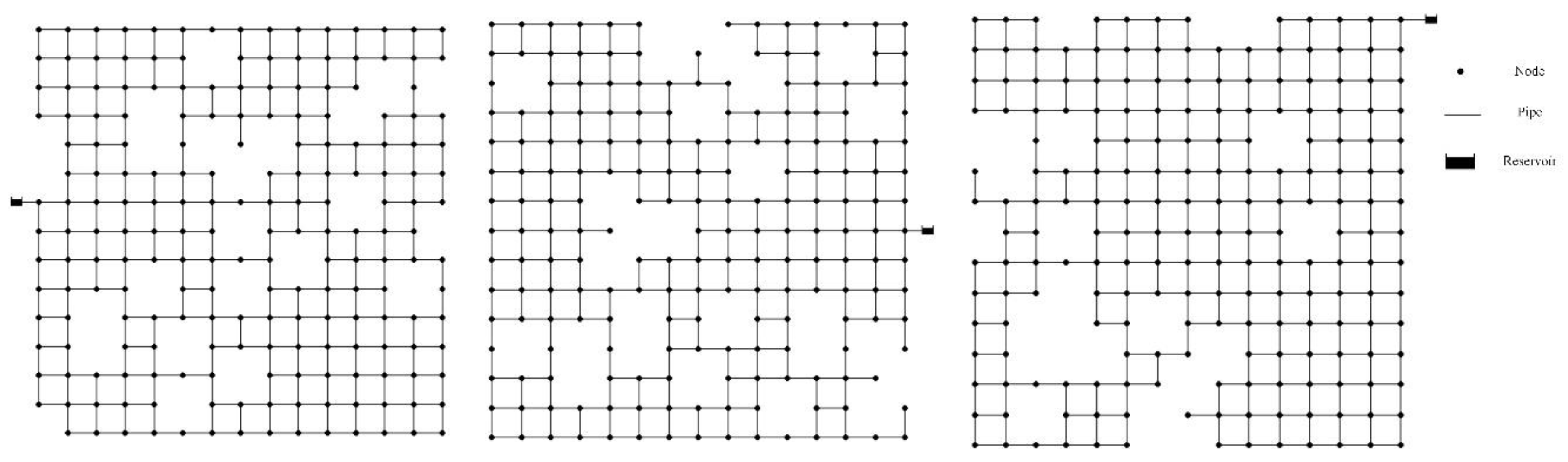
Figure 4.
Histogram of the N4 feature before (a) and after (b) outlier removal.
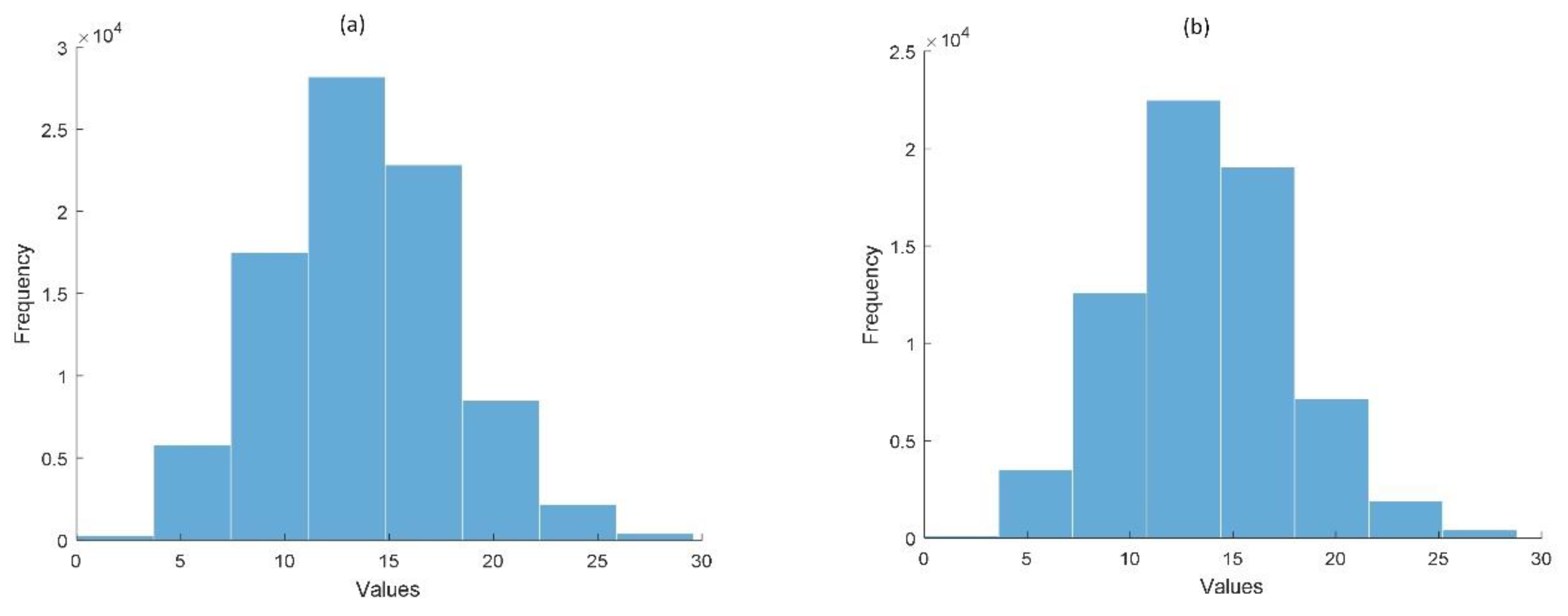
Figure 5.
The output of 24 coupled machine learning models.
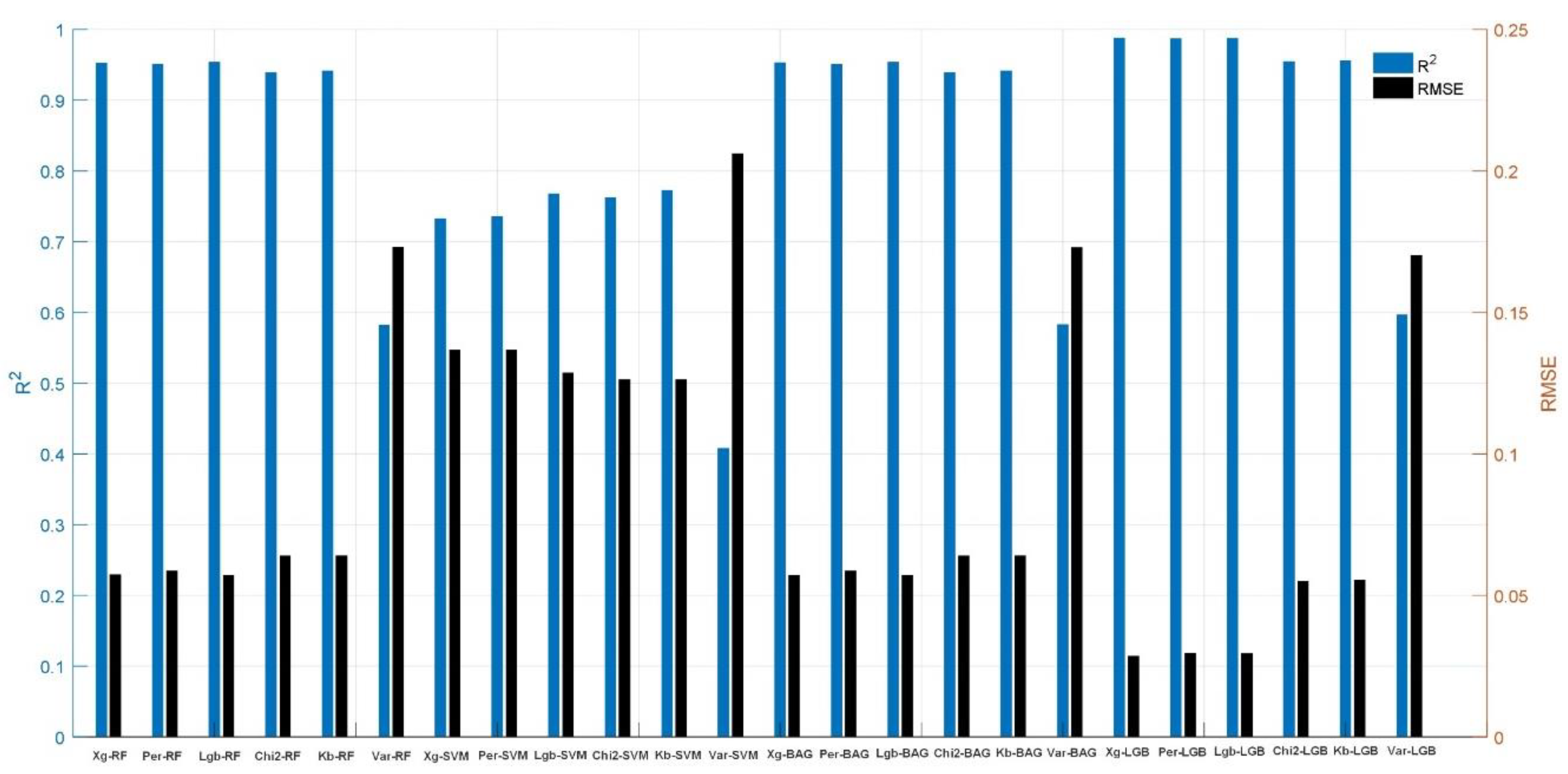
Table 1.
Commercial diameters and their corresponding costs.
| Diameter (mm) |
Cost of pipes (€) |
| 16 | 10.34 |
| 20 | 11.18 |
| 25 | 12.22 |
| 32 | 13.69 |
| 40 | 15.36 |
| 50 | 17.45 |
| 63 | 20.17 |
| 75 | 22.67 |
| 90 | 25.81 |
| 110 | 30.89 |
| 125 | 35.38 |
| 160 | 48.84 |
| 200 | 66.80 |
| 250 | 95.25 |
| 315 | 141.83 |
| 400 | 216.60 |
| 500 | 327.50 |
| 600 | 438.40 |
| 800 | 660.20 |
| 1000 | 882.00 |
Table 2.
The features obtained from synthetic WDNs.
| Network ID NO.1 |
Index NO.2 |
Graph Features NO.3 |
Node Features NO.4 |
Edge Features NO.5 |
Diameters NO.6 |
|||||||||
| G1 | G2 | … | G44 | N1 | N2 | … | N27 | E1 | E2 | … | E9 | |||
| Net 1 | Pipe1 | Net 1(G1) | Net 1(G2) | … | Net 1(G44) | P1N1 | P1N2 | … | P1N27 | P1E1 | P1E2 | … | P1E9 | Pipe1(D1) |
| Pipe2 | P2N1 | P2N2 | … | P2N27 | P2E1 | P2E2 | … | P2E9 | Pipe2(D2) | |||||
| … | … | … | … | … | … | … | … | … | … | |||||
| Pipen | PnN1 | PnN2 | … | PnN27 | PnE1 | PnE2 | … | PnE9 | Pipen(Dn) | |||||
| Net 2 | Pipe1 | Net 2(G1) | Net 2(G2) | … | Net 2(G44) | P1N1 | P1N2 | … | P1N27 | P1E1 | P1E2 | … | P1E9 | Pipe1(D1) |
| Pipe2 | P2N1 | P2N2 | … | P2N27 | P2E1 | P2E2 | … | P2E9 | Pipe2(D2) | |||||
| … | … | … | … | … | … | … | … | … | … | |||||
| Pipen | PnN1 | PnN2 | … | PnN27 | PnE1 | PnE2 | … | PnE9 | Pipen(Dn) | |||||
| … | … | … | … | … | … | … | … | … | … | … | … | … | … | … |
| Net 600 | Pipe1 | Net 600(G1) | Net 600(G2) | … | Net 600(G44) | P1N1 | P1N2 | … | P1N27 | P1E1 | P1E2 | … | P1E9 | Pipe1(D1) |
| Pipe2 | P2N1 | P2N2 | … | P2N27 | P2E1 | P2E2 | … | P2E9 | Pipe2(D2) | |||||
| … | … | … | … | … | … | … | … | … | … | |||||
| Pipen | PnN1 | PnN2 | … | PnN27 | PnE1 | PnE2 | … | PnE9 | Pipen(Dn) | |||||
Table 3.
First and last rows of extracted features from WDNs.
| Index | Graph Features | Node Features | Edge Features | Diameters (mm) |
|||||||||
| G1 | G2 | … | G44 | N1 | N2 | … | N27 | E1 | E3 | … | E9 | ||
| 0 | 379 | 407 | … | 3749 | 2.50 | 0.50 | … | 11.80 | 87 | 31 | … | 0.01 | 200 |
| 1 | 379 | 407 | … | 3749 | 2.50 | 1.00 | … | 11.90 | 108 | 71 | … | 0.00 | 600 |
| 2 | 379 | 407 | … | 3749 | 3.50 | 1.50 | … | 13.70 | 112 | 94 | … | 0.04 | 125 |
| 3 | 379 | 407 | … | 3749 | 3.00 | 1.00 | … | 11.90 | 112 | 22 | … | 0.00 | 500 |
| 4 | 379 | 407 | … | 3749 | 3.50 | 1.50 | … | 14.20 | 111 | 23 | … | 0.20 | 200 |
| 5 | 379 | 407 | … | 3749 | 2.50 | 1.00 | … | 15.20 | 114 | 29 | … | 0.22 | 50 |
| 6 | 379 | 407 | … | 3749 | 3.00 | 1.50 | … | 18.70 | 111 | 21 | … | 0.03 | 160 |
| 7 | 379 | 407 | … | 3749 | 3.00 | 1.50 | … | 18.90 | 111 | 22 | … | 0.00 | 800 |
| 8 | 379 | 407 | … | 3749 | 2.50 | 1.50 | … | 18.70 | 96 | 92 | … | 0.00 | 400 |
| 9 | 379 | 407 | … | 3749 | 3.50 | 2.00 | … | 18.50 | 96 | 78 | … | 0.00 | 315 |
| … | … | … | … | … | … | … | … | … | … | … | … | … | … |
| 85735 | 484 | 507 | … | 3672 | 3.00 | 0.50 | … | 28.80 | 120 | 46 | … | 0.00 | 250 |
| 85736 | 484 | 507 | … | 3672 | 3.00 | 1.50 | … | 36.50 | 118 | 54 | … | 0.30 | 40 |
| 85737 | 484 | 507 | … | 3672 | 3.00 | 1.50 | … | 45.00 | 106 | 63 | … | 0.03 | 250 |
| 85738 | 484 | 507 | … | 3672 | 3.00 | 1.00 | … | 46.30 | 87 | 38 | … | 0.02 | 315 |
| 85739 | 484 | 507 | … | 3672 | 3.00 | 1.50 | … | 52.20 | 88 | 49 | … | 0.22 | 90 |
| 85740 | 484 | 507 | … | 3672 | 3.00 | 1.50 | … | 58.80 | 91 | 40 | … | 0.06 | 315 |
| 85741 | 484 | 507 | … | 3672 | 3.00 | 1.50 | … | 63.80 | 92 | 89 | … | 0.08 | 315 |
| 85742 | 484 | 507 | … | 3672 | 3.00 | 2.00 | … | 68.20 | 83 | 45 | … | 0.03 | 1000 |
| 85743 | 484 | 507 | … | 3672 | 3.00 | 2.00 | … | 70.20 | 90 | 35 | … | 0.01 | 800 |
| 85744 | 484 | 507 | … | 3672 | 2.00 | 1.50 | … | 35.80 | 89 | 63 | … | 0.09 | 800 |
Table 4.
First and last rows of extracted features following outlier removal and normalization.
| Index | Graph Features | Node Features | Edge Features | Diameters (mm) |
|||||||||
| G1 | G2 | … | G44 | N1 | N2 | … | N27 | E1 | E3 | … | E9 | ||
| 0 | 0.23 | 0.04 | … | 0.41 | 0.25 | 0.00 | … | 0.13 | 0.17 | 0.14 | … | 0.01 | 0.19 |
| 1 | 0.23 | 0.04 | … | 0.41 | 0.25 | 0.20 | … | 0.14 | 0.70 | 0.64 | … | 0.00 | 0.59 |
| 2 | 0.23 | 0.04 | … | 0.41 | 0.75 | 0.40 | … | 0.16 | 0.80 | 0.92 | … | 0.07 | 0.11 |
| 3 | 0.23 | 0.04 | … | 0.41 | 0.50 | 0.20 | … | 0.14 | 0.80 | 0.02 | … | 0.00 | 0.49 |
| 4 | 0.23 | 0.04 | … | 0.41 | 0.75 | 0.40 | … | 0.16 | 0.77 | 0.04 | … | 0.38 | 0.19 |
| 5 | 0.23 | 0.04 | … | 0.41 | 0.25 | 0.20 | … | 0.17 | 0.85 | 0.11 | … | 0.44 | 0.03 |
| 6 | 0.23 | 0.04 | … | 0.41 | 0.50 | 0.40 | … | 0.22 | 0.77 | 0.01 | … | 0.06 | 0.15 |
| 7 | 0.23 | 0.04 | … | 0.41 | 0.50 | 0.40 | … | 0.22 | 0.77 | 0.02 | … | 0.00 | 0.80 |
| 8 | 0.23 | 0.04 | … | 0.41 | 0.25 | 0.40 | … | 0.22 | 0.40 | 0.90 | … | 0.01 | 0.39 |
| 9 | 0.23 | 0.04 | … | 0.41 | 0.75 | 0.60 | … | 0.21 | 0.40 | 0.73 | … | 0.00 | 0.30 |
| … | … | … | … | … | … | … | … | … | … | … | … | … | … |
| 85736 | 0.55 | 0.05 | … | 0.39 | 0.50 | 0.40 | … | 0.42 | 0.95 | 0.42 | … | 0.56 | 0.02 |
| 85737 | 0.55 | 0.05 | … | 0.39 | 0.50 | 0.40 | … | 0.52 | 0.65 | 0.54 | … | 0.06 | 0.24 |
| 85738 | 0.55 | 0.05 | … | 0.39 | 0.50 | 0.20 | … | 0.54 | 0.17 | 0.22 | … | 0.04 | 0.30 |
| 85739 | 0.55 | 0.05 | … | 0.39 | 0.50 | 0.40 | … | 0.61 | 0.20 | 0.36 | … | 0.44 | 0.07 |
| 85740 | 0.55 | 0.05 | … | 0.39 | 0.50 | 0.40 | … | 0.68 | 0.27 | 0.25 | … | 0.12 | 0.30 |
| 85741 | 0.55 | 0.05 | … | 0.39 | 0.50 | 0.40 | … | 0.74 | 0.30 | 0.86 | … | 0.17 | 0.30 |
| 85743 | 0.55 | 0.05 | … | 0.39 | 0.50 | 0.60 | … | 0.82 | 0.25 | 0.19 | … | 0.15 | 0.80 |
| 85744 | 0.55 | 0.05 | … | 0.39 | 0.00 | 0.40 | … | 0.41 | 0.22 | 0.54 | … | 0.17 | 0.80 |
Table 5.
Hyperparameter Values of Embedded Methods.
| Hyperparameter Tuning with Grid search | Embedded Methods | ||
| Xg | LGB | Per | |
| n-estimators | 1350 | 1500 | 1500 |
| eta | 0.250 | - | - |
| gamma | 0.002 | - | - |
| Max-depth | 15 | 12 | 12 |
| Num-leaves | - | 45 | 45 |
| Learning-rate | - | 0.011 | 0.011 |
Table 6.
Selection of top 20 features based on feature selection methods.
|
Methods Selected Features |
Kb | Chi2 | Var | LGB | Per | Xg | ||||||
| N5 | N5 | E1 | E9 | N5 | E9 | |||||||
| N7 | N7 | E3 | E8 | N7 | N5 | |||||||
| E5 | E5 | G43 | N5 | E3 | E8 | |||||||
| N8 | N8 | G44 | N7 | E9 | N7 | |||||||
| E9 | N17 | G7 | E3 | E1 | E1 | |||||||
| E3 | E9 | G20 | E1 | E5 | E3 | |||||||
| E1 | N15 | G21 | N8 | E8 | N8 | |||||||
| G42 | N19 | G23 | E5 | N8 | N10 | |||||||
| N23 | E8 | G30 | N10 | N10 | E5 | |||||||
| G12 | N18 | G31 | N6 | N6 | N6 | |||||||
| G8 | N2 | G32 | N4 | N3 | N26 | |||||||
| G4 | N10 | G35 | N17 | N17 | N4 | |||||||
| G17 | N3 | G36 | N26 | N1 | E6 | |||||||
| G13 | N13 | G39 | E4 | N23 | E7 | |||||||
| G10 | N6 | G41 | N19 | N25 | N17 | |||||||
| G41 | E3 | N1 | N9 | N4 | N20 | |||||||
| G6 | N4 | N2 | E6 | G25 | N15 | |||||||
| G18 | N14 | N5 | N18 | G3 | E4 | |||||||
| G27 | N22 | N7 | E7 | G2 | N9 | |||||||
| G2 | E1 | N23 | N20 | G10 | N19 | |||||||
| Node features percentage | 20 | 75 | 25 | 60 | 55 | 60 | ||||||
| Pipe features percentage | 20 | 25 | 10 | 40 | 25 | 40 | ||||||
| Over all graph features percentage | 60 | 0.0 | 65 | 0.0 | 20 | 0.0 | ||||||
Table 7.
Hyperparameter values of machine learning models.
| Hyperparameter tuning with Grid search | Ensemble model | |||
| RF | SVM | BAG | LGB | |
| n-estimators | 250 | - | 140 | 1500 |
| Max-depth | 30 | - | - | - |
| Min-samples-split | 10 | - | - | 12 |
| Max-samples | - | - | 0.7000 | - |
| Max-features | - | - | 0.7500 | - |
| C | - | 1.0000 | - | - |
| kernel | - | ‘ rbf ‘ | - | - |
| gamma | - | - | 0.0001 | - |
| Num-leaves | - | - | - | 45 |
| Learning-rate | - | - | - | 0.0110 |
Table 8.
The pipe diameters from Kadu and Xg-LGB models and pressure head in each node of Hanoi WDN.
Table 8.
The pipe diameters from Kadu and Xg-LGB models and pressure head in each node of Hanoi WDN.
| Pipe number | Predicted diameters | Node number | Pressure head from Xg-LGB model (m) | ||
| Pipe diameters from Kadu et al. (2008) (in) |
Continuous pipe diameters from Xg-LGB model (in) |
Commercial pipe diameters from Xg-LGB model (in) |
|||
| 1 | 40 | 38.9 | 40 | 1 | 100.00 |
| 2 | 40 | 36.9 | 40 | 2 | 97.14 |
| 3 | 40 | 40.7 | 40 | 3 | 61.67 |
| 4 | 40 | 40.3 | 40 | 4 | 57.39 |
| 5 | 40 | 39.9 | 40 | 5 | 52.09 |
| 6 | 40 | 39.5 | 40 | 6 | 46.56 |
| 7 | 40 | 39.1 | 40 | 7 | 45.29 |
| 8 | 40 | 40.0 | 40 | 8 | 43.83 |
| 9 | 30 | 33.7 | 30 | 9 | 42.69 |
| 10 | 30 | 35.4 | 40 | 10 | 39.40 |
| 11 | 30 | 34.9 | 30 | 11 | 39.01 |
| 12 | 24 | 27.4 | 30 | 12 | 37.85 |
| 13 | 16 | 18.2 | 20 | 13 | 36.44 |
| 14 | 12 | 14.0 | 16 | 14 | 37.81 |
| 15 | 12 | 13.0 | 12 | 15 | 37.66 |
| 16 | 16 | 18.4 | 20 | 16 | 38.17 |
| 17 | 20 | 22.1 | 24 | 17 | 45.01 |
| 18 | 24 | 24.4 | 24 | 18 | 51.52 |
| 19 | 24 | 28.2 | 30 | 19 | 60.16 |
| 20 | 40 | 40.0 | 40 | 20 | 51.41 |
| 21 | 20 | 23.4 | 24 | 21 | 47.56 |
| 22 | 12 | 13.1 | 12 | 22 | 42.40 |
| 23 | 40 | 39.2 | 40 | 23 | 45.98 |
| 24 | 30 | 34.6 | 30 | 24 | 41.44 |
| 25 | 30 | 34.4 | 30 | 25 | 38.72 |
| 26 | 20 | 21.4 | 20 | 26 | 36.67 |
| 27 | 12 | 14.1 | 16 | 27 | 36.69 |
| 28 | 12 | 14.6 | 16 | 28 | 39.30 |
| 29 | 16 | 17.6 | 16 | 29 | 36.26 |
| 30 | 12 | 14.5 | 16 | 30 | 36.26 |
| 31 | 12 | 13.0 | 12 | 31 | 36.47 |
| 32 | 16 | 17.6 | 16 | 32 | 36.74 |
| 33 | 20 | 23.9 | 24 | ||
| 34 | 24 | 26.8 | 24 | ||
Disclaimer/Publisher’s Note: The statements, opinions and data contained in all publications are solely those of the individual author(s) and contributor(s) and not of MDPI and/or the editor(s). MDPI and/or the editor(s) disclaim responsibility for any injury to people or property resulting from any ideas, methods, instructions or products referred to in the content. |
© 2025 by the authors. Licensee MDPI, Basel, Switzerland. This article is an open access article distributed under the terms and conditions of the Creative Commons Attribution (CC BY) license (http://creativecommons.org/licenses/by/4.0/).
Copyright: This open access article is published under a Creative Commons CC BY 4.0 license, which permit the free download, distribution, and reuse, provided that the author and preprint are cited in any reuse.


