Submitted:
07 April 2025
Posted:
08 April 2025
You are already at the latest version
Abstract
The growing interest in decentralized finance (DeFi), driven by advancements in blockchain technologies such as Ethereum, highlights the crucial role of smart contracts. However, the inherent openness of blockchains creates an extensive attack surface, exposing participants’ funds to undetected security flaws. In this work we investigate the use of deep reinforcement learning techniques, specifically Deep Q-Network (DQN) and Proximal Policy Optimization (PPO), for detecting and classifying vulnerabilities in smart contracts. This approach utilizes control flow graphs (CFGs) generated through EtherSolve to capture the semantic features of contract bytecode, enabling the reinforcement learning models to recognize patterns and make more accurate predictions. Experimental results from extensive public datasets of smart contracts reveal that the PPO model performs better than DQN and demonstrates effectiveness in identifying unchecked-call vulnerability. The PPO model exhibits more stable and consistent learning patterns and achieves higher overall rewards. This research introduces a machine learning method for enhancing smart contract security, reducing financial risks for users, and contributing to future developments in reinforcement learning applications.
Keywords:
blockchain
; decentralized finance
; smart contract
; reinforcement learning
1. Introduction
The rapid expansion of decentralized finance (DeFi) applications, especially on public blockchain platforms such as Ethereum, has significantly transformed the financial landscape [1]. Unlike conventional banking systems, DeFi utilizes the transparency and openness of decentralized networks, particularly blockchain technologies, to provide diverse financial services. However, the inherent openness of DeFi makes it highly susceptible to external attacks, posing serious risks to the security of participants’ funds. According to Kirişçi’s [2] study using the Fermatean fuzzy AHP approach to rank various risks in DeFi, technical risks are paramount, whereas financial risks are the most significant sub-risk, followed by transaction risks. On one hand, Solidity, the primary language for developing smart contracts, has certain design flaws that necessitate a strong focus on code security by developers. On the other hand, the immutable nature of blockchain technology means that deploying a vulnerable contract can result in irreversible financial losses.
Potential dangers arising from security vulnerabilities in DeFi can be enormous, as the ramifications extend beyond financial losses, encompassing broader systemic threats including diminished user trust [3]. A notable example is the 2016 DAO attack [4], where hackers exploited a vulnerability in a smart contract, stealing approximately $60 million in Ether, leading to a 40% drop in its market value. Another significant incident occurred in 2017 when Parity [5], an Ethereum wallet provider, lost around $270 million due to a vulnerability that destroyed a multi-signature wallet contract. More recently, in October 2022, a hacker exploited a cross-chain bridge vulnerability on the BNB Chain, resulting in the theft of 2 million BNB tokens, valued at approximately $566 million [6]. As of 2024, SlowMist [7] reports that cumulative losses from blockchain hacks have surpassed $3.5 billion. These recurring security breaches have severely impeded the development of the DeFi ecosystem and adversely affected stakeholders’ interests. Therefore, conducting thorough and precise security analyses of smart contracts prior to their deployment on Ethereum is crucial to minimize vulnerabilities, mitigate further security incidents, and safeguard users’ assets and trust in DeFi ecosystem.
Machine learning techniques have proven to be an effective approach for detecting security vulnerabilities in smart contracts. While traditional methods like static analysis and symbolic execution are used to identify issues such as reentrancy, integer overflows, and timestamp dependencies, these automated techniques are limited to detecting known vulnerabilities, are often time-intensive, and depend heavily on predefined rules from experts. As a result, machine learning and deep learning approaches have been developed to minimize the need for heavy feature engineering. Despite the growing success of supervised-learning-based detection methods, the exploration of reinforcement learning in smart contract vulnerability detection remains relatively underdeveloped in the existing literature.
To address the gap, this paper aims to apply reinforcement learning techniques to the process of smart-contract vulnerability detection and conducting an empirical analysis with a substantial dataset.
The main contributions of this paper are as follows:
- We design and implement a reinforcement learning architecture for detecting and classifying smart contract vulnerabilities and show its viability through a comparison analysis.
- Based on the characteristics of smart contract bytecode, we propose CFGs, a graph-base method for input representations to capture richer semantic information within the bytecode.
- We propose a machine learning approach for improving blockchain security and future reinforcement learning applications.
The rest of the paper is organized as follows. Section 2 provides a comprehensive review of the research work related to this paper. In Section 3, we elaborate the data work in the analysis and the methodology for building feature representations and model architectures. Section 4 examines and discusses the experimental results, and Section 5 summarizes and highlights possible future research work.
2. Related Works
Extensive research of formal methods has been conducted on the detection of vulnerabilities in smart contracts by earlier times. Traditional methods, distinguished by the software testing techniques utilized, can be classified into four categories: symbolic execution, formal verification, fuzz testing and static analysis [8]. Symbolic execution is first used in automated analysis tool such as Oyente [9] and Mythril [10] for Ethereum smart contracts, where it simulates all possible execution paths on contract codes and detecting potential vulnerabilities but may face difficulty when analyzing complex contracts. The formal verification tool Securify [11] and static analysis tools such as SmartCheck [12] and Slither [13] improve the efficacy of addressing complex issues by adopting a specialized domain-specific representation to describe compliance and violation patterns, thereby facilitating the identification of potential security flaws. However, it may overlook new vulnerabilities that do not conform to known patterns. Numerous dynamic analysis tools, including ReDefender [14] and ConFuzzius [15], have gained popularity as the fuzz testing technique develops. These tools generate fuzzing inputs and verify vulnerabilities through dynamic data dependency analysis, but their detection scope is restricted to a narrow of vulnerability types.
Traditional tools predominantly depend on predefined hard logic rules established by experts for detecting vulnerabilities. However, as smart contract technology advances, these tools are becoming insufficient to meet contemporary requirements due to below limitations [16].
- The complexity of smart contract structures and functionalities is increasing. As the variety of vulnerabilities in smart contracts continues to grow, expert-defined rules based on existing vulnerability definitions struggle to keep pace with these updates.
- Smart contracts may demonstrate varied behaviors at runtime depending on different conditions, complicating the process of vulnerability verification and rendering the analysis highly resource- and time-consuming due to their dynamic and conditional nature.
In recent years, machine learning-based approaches for detecting vulnerabilities in smart contracts have garnered extensive attention and research, as a higher accurate and efficient results are achieved during smart-contract security analysis. Within this field, supervised learning techniques have particularly made significant progress and are widely applied in real-world scenarios, including the web service tool SmartEmbed [17] for detecting repetitive code and clone-related bugs, the support vector machine embedded scanning system SCScan [18], a tree-based approach using an improved CatBoost algorithm for early detection of Ponzi Smart Contracts on Ethereum [19]. More deep learning approaches have emerged since 2020. The bidirectional Long Short-Term Memory networks enhance detection accuracy for reentrancy vulnerabilities and reduces the occurrence of false positives by incorporating contract snippet representations and attention mechanisms [20,21]. And convolutional neural network and graph neural network architectures are used to detect vulnerabilities in smart contracts and achieve over 80% accuracy by maintaining the semantic and contextual information under abstract syntax trees representations [22,23]. There also emerges specialized bidirectional encoder representations from transformers models for smart contract vulnerability detection to mitigate the challenge of insufficient labelled data [24,25].
While supervised learning techniques have yielded notable successes in the detection of smart contract vulnerabilities, reinforcement learning approaches have received relatively less attention and exploration in this field. Andrijasa et al.’s [26] review paper proposed a deep reinforcement learning with multi-agent fuzzing for exploit generation on cross-contract, and Su et al. [27] introduced a novel reinforcement learning fuzzer (RLF) a year later, which utilized reinforcement learning to guide fuzzing for generating vulnerable transaction sequences in smart contracts and effectively detecting sophisticated vulnerabilities requiring specific transaction sequences. However, RLF merely investigated the efficiency of detecting Ether-Leaking and Suicidal vulnerabilities, and the dataset used for training RLF consists of just 1,291 entries, which may restrict the generalizability and reliability of reinforcement learning methods.
This paper seeks to address the aforementioned challenges and other undisclosed gaps by applying deep reinforcement learning algorithms to the vulnerability detection task and utilizing a more comprehensive dataset for model training.
3. Materials and Methods
3.1. Data
3.1.1. Data Description
The dataset adopted in this study was obtained from the public dataset released by Rossini et al. [28] on HuggingFace [29]. Combined with other open-source datasets sorted in earlier research, this dataset is extensive, high-quality, and includes over 100,000 entries from active contracts on the Ethereum main net, where the source code of every contract was obtained via Etherscan API [30] and bytecode was retrieved using `web3` Python package.
Entries in this dataset are labelled as each contract’s code is verified by the Slither static analyzer to detect its vulnerability type. It has been mapped to the following five categories.
- Access-control: This vulnerability occurs when smart contracts inadequately enforce permission controls, enabling attackers to perform unauthorized actions. It contains several subclasses. 1) Suicidal: This refers to contracts that include functions capable of terminating the contract and transferring its funds; 2) Arbitrary-send: Code loophole leading to Ether loss when the contract sends Ether to arbitrary addresses; 3) tx.origin: Relying on `tx.origin` for authentication can be risky as it may enable attacks where a malicious contract can impersonate the original sender; 4) Controlled-delegatecall: Security issue that arises when a contract improperly uses the delegatecall() function.
- Arithmetic: This class is related to Integer underflow and overflow errors as well as Divide-before-multiply error where division is done before multiplication.
- Reentrancy: A security issue occurs when a contract allows an external call to another contract before it resolves the initial call, potentially allowing an attacker to drain funds or exploit the contract’s state. This type of vulnerability can be further classified as Reentrancy-no-eth where attacks do not involve Ether and Reenthrancy-eth where attacks involve Ether transfers.
- Unchecked-calls: This class refers to a security issue that arises when a contract makes an external call to another contract or address without properly checking the success of that call. It includes three main types, which are Unused-return, Unchecked-low level and Unchecked-transfer calls.
- Other vulnerabilities: 1) Uninitialized-storage: Storage pointers that are not initialized can redirect data to unexpected storage slots; 2) Mapping-deletion: The belief that deleting a mapping deletes its contents; 3) Time dependency: a smart contract depends on the block timestamp or block number where time-related values can be influenced or predicted to some extent by miners, leading to potential manipulation; 4) Constant-function-state: Functions marked as constant/view that can modify state lead to unexpected behaviors; 5) Array-by-reference: Passing arrays by reference can lead to unexpected side effects if they’re modified.
3.1.2. Data Preparation
With basic data cleaning done, we then expanded the list-type labels across multiple rows, as a single contract may exhibit multiple types of vulnerability in practice. Table 1 illustrates the distribution of contracts across each vulnerability class in our training set. A notable observation is the significant class imbalance, with the unchecked-calls, safe, and reentrancy classes being the most prevalent, whereas the access-control vulnerability class is underrepresented and contains only about 1.1 thousand smart contracts, making it the minority class.
The dataset was split into training, validation, and test sets while preserving the class distribution. The final splits consist of approximately 134k entries for training, 18k for validation, and 27k for testing. As shown in Figure 1, although the vulnerability classes are imbalanced, their distribution remains proportionally consistent across all subsets, as expected.
Lastly, we eliminated duplicate rows and dropped elements for which the bytecode was not available before forming reinforcement learning environment.
3.2. Control Flow Graphs
The key concept in the feature engineering process is the generation of control flow graphs. Rather than utilizing decompiled raw opcode in a sequence level to retain semantic information of how the contract operates within Ethereum Virtual Machine, this paper leverages graph representation approach for bytecode parsing. CFGs are often preferred over raw opcode of bytecode as input representations for reinforcement learning (RL) methods because CFGs provide a structured and high-level abstraction of the program’s execution flow. A CFG captures the possible paths that might be traversed through a program during its execution, which allows for a more comprehensive understanding of the logical flow and control dependencies within the code. This is particularly important in detecting vulnerabilities in smart contracts, where understanding the control flow can reveal critical insights into how different parts of the contract interact and where potential security flaws might locate. Also, RL algorithms like PPO rely on the environment’s state representation to learn optimal policies. When the state space is well-structured, as with CFGs, the learning process becomes more efficient and effective.
However, the inherent complexity of Ethereum bytecode, particularly in jump resolution, presents substantial challenges for static analysis and reduces the accuracy of extraction of CFGs by existing automated tools. EtherSolve, introduced by Contro et al. [31], provided a novel static analysis tool leveraging symbolic execution of the Ethereum operand stack. This approach enables the resolution of jumps within Ethereum bytecode, facilitating the construction of accurate CFGs for compiled smart contracts. The CFG is a directed graph that illustrates the execution flow within a program, where nodes represent the program’s basic blocks—sequences of opcodes that lack jumps except in the final opcode—while edges connect potential successive basic. The process of generating a CFG is detailed through a series of steps below.
- Bytecode parsing. It begins by identifying and removing the metadata section of the raw bytecode, followed by parsing the remaining bytes into opcodes.
- Basic block identification. A basic block is a sequence of opcodes executed consecutively without any other instructions altering the flow of control. Specific opcodes JUMP (unconditional jumps), JUMPI (conditional jumps), STOP, REVERT, RETURN, INVALID and SELFDESTRUCT, mark the end of a basic block, while JUMPDEST marks the start.
- Symbolic stack execution. This step is used to resolve the destinations of orphan jumps during CFG construction. Orphan jumps are common in smart contracts, especially when a function call returns, and their destinations need to be determined. The approach involves symbolically executing the stack by focusing only on opcodes that interact with jump addresses (PUSH, DUP, SWAP, AND and POP), while treating other opcodes as unknown.
- Static data separation. It involves removing static data from the CFG by identifying and excluding sections of the code that are not executable. This is done by detecting the 0xFE opcode, which marks the transition from executable code to static data with representation for invalid instruction, and subsequently removing any unconnected basic blocks from the graph.
- CFG decoration. It involves adding additional information to the control flow graph to make it more useful for analysts and subsequent static analysis tasks (e.g., for vulnerability detection). Specifically, EtherSolve highlights important components of the CFG, such as the dispatcher, fallback function, and final basic block.
This paper utilizes EtherSolve.jar, sourced from Github [32], to generate control flow graphs from the bytecode of smart contracts. The generated CFGs are stored in .dot format for features extraction, which is subsequently used to feed reinforcement learning agents. Figure 2 shows a partial CFG for one contract from the training set.
3.3. Model Architectures
Reinforcement learning centers on the decision-making process, where agents interact with their environment to maximize the rewards they receive. This paper implements two model-free reinforcement learning algorithms that are Deep Q-Network (DQN) and PPO, where “model-free” indicates the agent has no access to a model of the environment.
3.3.1. Deep Q-Network
DQN is an off-policy reinforcement learning algorithm that combines Q-learning with deep neural networks. According to Mnih et al. [33], DQN agents can often be simulated through the probability distribution function derived from the state-value function in the action space or the scoring rules of the action-value function in the action space. This study uses agents that rely on action-value functions to define the vulnerability detection logic. Here, the agent can be mathematically modelled by where represents the action at time , denotes the state at time . The agent acts like a prophet to evaluate each action in the action space based on the current state, thereby making optimal decisions at each moment to maximize the reward during the progress. In the Q-learning algorithm, the agent is formed using a Q-table to store all actions across various states. However, in a real-world problem such as vulnerability detection in smart contracts, the vast number of states poses a challenge for Q-tables to manage effectively. To address this, the improved DQN utilizes deep neural networks to approximate Q-tables for constructing agents by taking a state as input and outputting Q-values for all possible actions (Figure 3) [34]. This allows the algorithm to handle high-dimensional state spaces, such as images or graphs.
The training process for agent in Q-learning relies on the algorithm of temporal difference (TD) in Equation 1, where is learning rate, represents discount factor, indicates the action taken by the Q-learning agent.
In the DQN framework, the TD equation is employed to update the parameters of the neural network. Instead of learning from consecutive samples, DQN uses a replay buffer to store the agent’s experiences. Specifically, the replay buffer records state transitions, selected actions, and the corresponding immediate rewards from each agent-environment interaction, forming a tuple . During training, mini-batches of experiences are randomly sampled from the buffer to update the Q-network. This technique helps to break the correlation between consecutive samples and leads to more stable training. This approach leads to the definition of the DQN objective function as in Equation 2, where is the vector of parameters of agent .
In this paper, the procedure for employing DQN agents in vulnerability detection is outlined as follows: begin at time , the pair set of CFG’s node and edge is initialised and fill in the data inputs. An action is randomly selected to establish the initial state . Subsequently, for in , the agent chooses the action that yields the highest score based on the function and executes this action within the environment. Following this, the agent receives the immediate reward from the environment and observes the subsequent state ,updating the agent’s parameter vector accordingly, leading to the formation of the next state . This procedure is repeated until the environment reaches the terminal state . The primary objective of the agent is to maximise the cumulative return of . The specific algorithm for using neural network to train the agent can be found in Algorithm 1.
| Algorithm 1. DQN with Replay Buffer |
| Initialize experience replay buffer to capacity |
| Initialize Q-network with random weights Initialize a target network where Set action space for six possible class labels For episode = 1, do: Initialize state from first observation of CFG features For step to do: With probability select a random action or select action Execute action on the environment (i.e., predict vulnerability type) Observe reward and next state Store state transition in replay buffer Randomly sample minibatch of transition tuple from Set or if episode ends at step Perform a gradient descent step on loss for Set for every C step end for end for |
3.3.2. Proximal Policy Optimization
Unlike the off-policy DQN, PPO is an on-policy reinforcement learning algorithm that relies heavily on policy gradients where the key idea is to push up the probabilities of actions that lead to higher return, in the meantime push down the probabilities of actions that lead to lower return, until it arrives at the optimal policy. Under normal policy gradient, it keeps new and old policies close in parameter space. However, since even minor variations in parameter space can result in significant performance differences, a single bad step can collapse the policy performance. This risk makes large step sizes particularly dangerous when applying vanilla policy gradients, thereby hurting the sample efficiency. To address the challenge, an improved PPO algorithm firstly introduced by Schulman et al. [35] from OpenAI [36], refines policies by taking the largest step possible to enhance performance, while adhering to a constraint that ensures the new policy remains sufficiently similar to the previous one. This paper implements the clip version of PPO, which uses specialized clipping (positive or negative advantage) instead of KL-divergence in the objective function to remove incentives for the new policy to get far from the old policy.
Let denote a policy with parameter , and denote the expected finite-horizon undiscounted return of the policy. The gradient of can be defined as:
where is a trajectory and is the advantage function for the current policy.
PPO-clip updates policies via:
which takes multiple steps of minibatch size to maximise the objective. Here is given by:
Where
in which represents a (small) hyperparameter that dictates the permissible deviation of the new policy from the old.
To derive meaningful insights from this clipping setup, let’s focus on a specific state-action pair , and think of cases.
- Advantage is positive: Suppose the advantage for that state-action pair is positive, its contribution to the objective function diminishes to:
Since the advantage is positive, the objective will increase if the action becomes more likely, i.e., if increases. However, the function in this expression imposes a cap on how much the objective can rise. Once exceeds , the minimum constraint activates, causing the term to reach a ceiling of . Consequently, the new policy does not gain further benefit by diverging significantly from the previous policy.
- Advantage is negative: Suppose the advantage for that state-action pair is negative, its contribution to the objective function diminishes to:
Since the advantage is negative, the objective will increase if the action becomes less likely, i.e., if decreases. However, the function in this expression imposes a cap on how much the objective can rise. Once falls below , the maximum constraint activates, causing the term to reach a ceiling of . Consequently, again, the new policy does not gain further benefit by diverging significantly from the previous policy.
In this study, PPO-clip algorithm is utilized to train a stochastic policy using an on-policy approach, where it explores by sampling actions based on the most recent iteration of its stochastic policy. The degree of randomness in action selection (the vulnerability type) is influenced by initial conditions and the training process. As training progresses, the policy tends to become less random since the update mechanism encourages the exploitation of rewards that have already been found. However, one drawback of PPO is that this process may cause the policy to get trapped in local optima. The full details can be found in Algorithm 2 below.
| Algorithm 2. PPO-Clip |
| Initialize policy parameter |
| Initialize value function parameters For do: Collect set of trajectories by running policy in the environment Compute rewards-to-go Compute advantage estimates based on current value function Update the policy by maximising the PPO-Clip objective: typically via stochastic gradient ascent with Adam Fit value function by regression on mean-squared error: typically via some gradient decent algorithm end for |
3.4. Model Configurations
3.4.1. Agent Environment
To ensure the reinforcement learning agent performs well, it is necessary to set up a custom environment tailored to the classification task as formed in this paper. It involves constructing the action and observation spaces, implementing functions to retrieve the current observation and transition between states, and incorporating a function to compute the immediate reward. After setup, apply the training, validation and test sets to the environment. The complete framework for environment setup is detailed in Algorithm 3.
| Algorithm 3. Agent Environment Setup |
| class SmartContractEnv() |
| function extract_features_from_cfg() Extract graph features from .dot file of CFGs function __init__() Initialize current step as Initialize action space as to capture six classes Initialize observation space as feature shape of extract_features_from_cfg() function _get_observation() Extract the CFG features for the current contract function step() Set current step forward while episode not done, do: Set next state by _get_observation() Calculate reward by _calculate_reward () end while function _calculate_reward() Define the reward calculation rules as: when action matches true labels, get a reward 1 Initialize environments to training, validation and test sets by SmartContractEnv() |
3.4.2. Hyperparameter Tuning
Hyperparameter tuning is a critical aspect of optimizing reinforcement learning algorithms like DQN and PPO because it directly influences the model’s performance and convergence. In reinforcement learning, hyperparameters control various aspects of the learning process, such as how quickly the model adapts to changes (learning rate), the size and management of experience replay buffers (buffer size etc.), how actions are selected (gamma), and the frequency and the way updates are made (batch size, steps, epochs). In this paper, the following hyperparameters are considered for tuning:
- Learning rate: This parameter controls how much the model updates its knowledge after each step. A too-high learning rate might cause the model to overlook optimal solutions, while a too-low rate may result in slow learning and the model getting stuck in local optima.
- Batch size: Size of the minibatch for training. Larger batch sizes generally lead to more stable updates but require more computational resources.
- Gamma: The discount factor belonging to (0,1) that represents the importance of future rewards. A gamma close to 1.0 makes the model value long-term rewards, while a smaller gamma makes it prioritize immediate rewards.
- Steps before learning (DQN specific): This defines how many steps of the model to collect transitions for before learning starts. Delaying learning can help the model accumulate a diverse set of experiences, improving the stability and performance of the learning process.
- Buffer size (DQN specific): Size of the replay buffer that stores past experiences for the model to learn. A larger buffer allows the model to learn from a broader range of experiences but may increase memory usage and slow down training.
- Number of steps (PPO specific): The number of steps to run for each environment per update. More steps can stabilize the model by providing more data for each update but may also slow down the learning process.
- Number of epochs (PPO specific): This specifies how many times the model iterates over the data to optimize the policy during each update. More epochs can lead to better policies but can also increase the risk of overfitting.
- Entropy coefficient (PPO specific): Entropy coefficient for the loss calculation. Higher coefficient can promote exploration and help in avoiding local minima.
- Clip range (PPO specific): Clipping parameter, it can be a function of the current progress remaining (from 1 to 0). In PPO, the clip range limits how much the policy can change during training, which helps maintain the balance between exploring new policies and retaining what has already been learned.
3.5. Evaluation Metrics
Considering that the objective of this study is formed as a multi-label classification task with an imbalanced dataset, we adopted three primary metrics to evaluate our models, which are Accuracy, Micro-Recall and Micro-F1. The ROC curve and Precision-Recall (PR) curve are also implemented to evaluate the model performance across classes using One-Vs-All methodology.
- Label Accuracy: it measures the proportion of correct predictions for each label across all instances. Formally, denote as the true label value (either 0 or 1) of the th label for the th sample, and as its predicted label value. Label accuracy can be defined as:
- Subset Accuracy: a stricter accuracy score that measures the proportion of instances where all labels are correctly predicted. The mathematical formulation is:
- Micro-Recall: Recall measures the proportion of correctly identified out of all actual positives. For micro-level evaluation, labels from all samples are merged into a single comprehensive set. The recall is then calculated based on this aggregated set with following formula:
- Micro-F1: The F1 score is the harmonic mean between Precision and Recall, bounded between 0 and 1. At the micro-level, the F1 score can be calculated as:
where
- Learning curve: The learning curve plots the model’s performance (in our case the reward) against the number of training iterations or episodes. It helps to visualize the learning process, showing how quickly the model learns and how well it generalizes to new data.
- Receiver operating characteristic (ROC) curve: The ROC curve is a visual tool used to assess a classification model’s effectiveness by illustrating the relationship between the True Positive Rate (TPR) and the False Positive Rate (FPR). TPR reflects the percentage of actual positives that the model correctly identifies, while FPR represents the percentage of negatives mistakenly classified as positives. An ideal ROC curve would rise along the y-axis towards the upper left corner, indicating high TPR and low FPR. The Area Under the ROC curve (AUC) provides an overall performance metric for the model. AUC values range from 0 to 1, with values near 1 indicating superior model performance, and those around 0.5 suggesting performance comparable to random guessing. In a multi-label classification task, One-Vs-All methodology is adopted to plot the ROC curve.
- Precision-Recall (PR) curve: The PR curve is particularly insightful when dealing with imbalanced datasets, where the positive class is rare. It focuses on the precision (positive predictive value) and recall (sensitivity) of the model, providing a clear view of the trade-off between these two metrics. By adjusting this threshold, different combinations of precision and recall can be achieved, which are then visualized on the PR curve. Lowering the threshold typically increases the likelihood of predicting positive instances, which may result in more false positives, thus reducing precision but raising recall. Conversely, raising the threshold makes the model more selective, leading to fewer false positives and higher precision, but potentially at the cost of reduced recall. Ideally, a model would achieve both high precision and recall, with the PR curve nearing the top-right corner of the graph. The area under the PR curve (AUC-PR) serves as a single summary metric, with higher values indicating better performance.
4. Experiment and Analysis
In this study, our experiments were conducted on GPU nodes from a high-performance computing facility. Each node was equipped with two NVIDIA Tesla V100 GPUs (16GB HBM2 memory each), 64GB of DDR4 RAM, and an 8-core Intel Xeon E5-2698 v4 CPU.
Experiments in this section begins by evaluating the performance of reinforcement learning models using three metrics during validation phase, accompanied by an analysis of their learning curves. Following the evaluation, the optimal one will be selected and deployed to the test set for effectiveness examination. The section concludes by discussing the experimental results.
4.1. Evaluation of RL Model Performance
Table 4 presents the validation metrics for DQN and PPO performances. Both models underperformed in this multi-label classification task, achieving only 18.69% and 29.47% accuracy, respectively. A likely contributing factor to these suboptimal outcomes is the limited data available for each class. The training set, consisting of 13,400 elements across six classes, resulted in insufficient data per class, which may hinder the models’ predictive capabilities. This limitation is particularly significant given that the models were trained from scratch using high-level semantic features from control flow graphs, which typically require large datasets for effective training. Notably, the PPO model outperformed the DQN model, demonstrating superior accuracy, recall, and F1 score.
Moreover, learning curves can be further plotted to evaluate the learning process for both models (Figure 7). The DQN learning curve shows a high frequency of low rewards with many episodes having rewards close to 1.0 and a sparse high reward pattern, suggesting that the DQN model is struggling to consistently learn an action that results in higher rewards, and it may not be converging well or may be experiencing significant variance in the learning process. On the other hand, the PPO learning curve shows a more gradual increase in rewards over episodes with rewards are generally higher compared to the DQN model. While there is some fluctuation in rewards, this is normal and suggests the model is exploring different strategies. The general trend appears to be upward, indicating that the PPO model is learning and improving its policy. To sum it up, the PPO model seems to be more stable than the DQN model as the curve is smoother and shows more consistency in achieving higher rewards, which is typical of PPO due to its on-policy nature and the way it optimizes the policy.
4.2. Evaluation of RL Model Effectiveness
Based on the validation performance, the PPO model is selected as the optimal model and subsequently deployed on the test set, with the classification report summarized in Table 5. The accuracy stands at 30%, which is consistent with the accuracy observed on the validation set, indicating the stability of the PPO model. However, the predictive performance varies significantly across different classes. The recall for unchecked-calls is notably high at 0.81, with an F1 score of 0.46, the highest among all classes. Safe class follows, achieving an F1 score of 0.19. The remaining four classes exhibit suboptimal prediction performance. This outcome is consistent with the dataset’s characteristics identified during data preparation, where a pronounced class imbalance was observed, with the ratio of unchecked-calls to access-control classes being approximately 3:1. Given that nearly half of the contracts fall within the unchecked-calls and safe classes, these categories have a substantial amount of data available for training the reinforcement model, leading to better predictive performance for these classes.
To visualize the model effectiveness among various vulnerability categories, both the ROC curve and the Precision-Recall (PR) curve were plotted for analysis (Figure 4). The ROC curve reveals similarly suboptimal model performance across six classes, with the Area Under the Curve (AUC) values hovering around 0.55. However, in the case of imbalanced datasets where positive class is infrequent, the ROC curve can be misleading, as it might indicate high performance even if the model performs poorly on the positive class. Thus, the PR curve offers a more insightful evaluation for our task, as it focused on the positive class (i.e., the vulnerability class) and aims to mitigate the significant costs associated with false positives (i.e., falsely detecting vulnerabilities). The results align with the classification report, as the area under the PR curve for unchecked-calls stands at 0.78, indicating that the model demonstrates moderate effectiveness when predicting the majority class.
4.3. Discussion
Despite the creative effort in applying reinforcement learning algorithms to vulnerability detection, there are still some limitations faced by this study and directions for future research. One significant limitation lies in the use of a limited dataset for training the reinforcement learning models. This limitation hinders the models’ ability to adequately learn patterns across individual classes. This research primarily relies on CFGs to extract high-level semantics from contract bytecode. However, other graph representations, such as abstract syntax tree and program dependency graph, may offer richer syntactic and semantic insights.
5. Conclusions
This paper shows that reinforcement learning techniques could be a viable tool for detecting and classifying smart contract vulnerabilities. Utilizing a publicly sourced dataset, two distinct model architectures are trained and evaluated. Treating vulnerability detection as a multi-label classification problem, graph representations are generated to capture relevant semantic features from the contract bytecode. The results indicate that, given the configurations in terms of custom environment setup and hyperparameter tuning, the PPO model exhibits more stable and consistent learning patterns and achieves higher overall rewards. When applied to the test set, the PPO model displays effectiveness, particularly for the majority class of vulnerabilities, as evidenced by metrics such as Micro Recall, Micro F1, and the PR curve. The findings of this study offer valuable insights that may encourage scholars and developers to explore the potential of reinforcement learning techniques for improving smart contract security and mitigating financial risks for DeFi stakeholders.
Supplementary Materials
The code is provided at https://github.com/jjdlg361/SmartContractRL
Author Contributions
Conceptualization, Ravji; methodology, Zhang, de Leon and Koulouris; software, de Leon, Koulouris and Zhang; validation, de Leon, Koulouris; investigation, de Leon, Koulouris and Zhang, Medda, Ravji; resources, de Leon; data curation, de Leon Jose Juan; writing—original draft preparation, de Leon, Koulouris and Zhang, Medda, Ravji; writing—review and editing, de Leon, Koulouris and Zhang, Medda, Ravji; visualization, de Leon, Koulouris and Zhang.; supervision, Medda and Ravji; project administration, Medda. All authors have read and agreed to the published version of the manuscript.
Funding
This research received no external funding.
Data Availability Statement
The dataset adopted in this study was obtained from the public dataset released by Rossini et al. [28] on HuggingFace [29]. Combined with other open-source datasets sorted in earlier research, this dataset is extensive, high-quality, and includes over 100,000 entries from active contracts on the Ethereum main net, where the source code of every contract was obtained via Etherscan API [30] and bytecode was retrieved using `web3` Python package.
Conflicts of Interest
The authors declare no conflicts of interest.
Abbreviations
The following abbreviations are used in this manuscript:
| DeFi | Decentralized Finance |
| DQN | Deep Q-Network |
| PPO | Proximal Policy Optimization |
| CFG | Control Flow Graph |
| CFGs | Control Flow Graphs |
| RLF | Reinforcement Learning Fuzzer |
| RL | Reinforcement Learning |
| ROC | Receiver Operating Characteristic |
| PR | Precission-Recall |
| TPR | True Positive Rate |
| FPR | False Positive Rate |
References
- Wood, G. Ethereum: A Secure Decentralized Generalised Transaction Ledger. Ethereum Project Yellow Paper 2014, 151, 1–32. [Google Scholar]
- Ki̇ri̇şçi̇, M. A Risk Assessment Method for Decentralized Finance(DeFi) with Fermatean Fuzzy AHP Approach. Advances in transdisciplinary engineering 2023, 42, 1215–1223. [Google Scholar] [CrossRef]
- De Baets, C. , Suleiman, B., Chitizadeh, A. and Razzak, I. Vulnerability Detection in Smart Contracts: A Comprehensive Survey. arXiv: Cryptograophy and Security. [CrossRef]
- Mehar, M. , Shier, C.L., Giambattista, A., Gong, E., Fletcher, G., Sanayhie, R., Kim, H.M. and Laskowski, M. Understanding a revolutionary and flawed grand experiment in blockchain: The DAO attack. Journal of Cases on Information Technology. [CrossRef]
- Breidenbach, L. , Daian, P., Juels, A., Sirer, E.G. An in-depth look at the parity multisig bug’. Hacking 2017. [Google Scholar]
- Explained: The BNB Chain Hack (October 2022). Available online: https://www.halborn.com/blog/post/explained-the-bnb-chain-hack-october-2022 (accessed on 15 March 2025).
- SlowMist. Available online: https://hacked.slowmist.io/ (accessed on 12 March 2025).
- Piantadosi, V. , Rosa, G., Placella, D., Scalabrino, S. and Oliveto, R. Detecting functional and security-related issues in smart contracts: A systematic literature review. Software: Practice and Experience. [CrossRef]
- Luu, L. , Chu, D. H., Olickel, H., Saxena, P. and Hobor, Vienna, Austria, 24 October 2016., A. Making smart contracts smarter’. In Proceedings of the 2016 ACM SIGSAC Conference on Computer and Communications Security. [Google Scholar] [CrossRef]
- Prechtel, D. , Groß, T. In and Müller, T. (2019). Evaluating Spread of ‘Gasless Send’ in Ethereum Smart Contracts. In Proceedings of the 2019 10th IFIP International Conference on New Technologies, Mobility and Security (NTMS) Canary Islands, Spain, 24-26 June 2019. [Google Scholar] [CrossRef]
- Tsankov, P. , Dan, A. , Drachsler-Cohen, D., Gervais, A., Bünzli, F. and Vechev, In Proceedings of the 2018 ACM SIGSAC Conference on Computer and Communications Security, Toronto, Canada, 15 October 2018., M. Securify: Practical Security Analysis of Smart Contracts. [CrossRef]
- Tikhomirov, S. , Voskresenskaya, E. , Ivanitskiy, I., Takhaviev, R., Marchenko, E. and Alexandrov, Gothenburg, Sweden, 27 May 2018., Y. SmartCheck: static analysis of ethereum smart contracts. In Proceedings of the 1st International Workshop on Emerging Trends in Software Engineering for Blockchain. [CrossRef]
- Feist, J. , Grieco, G. and Groce, A. Slither: A Static Analysis Framework For Smart Contracts. 2019 IEEE/ACM 2nd International Workshop on Emerging Trends in Software Engineering for Blockchain (WETSEB), 8–15. [CrossRef]
- Li, B. , Pan, Z. and Hu, T. ReDefender: Detecting Reentrancy Vulnerabilities in Smart Contracts Automatically. IEEE Transactions on Reliability. [CrossRef]
- Torres, C. F. , Iannillo, A. K., Gervais, A. and State, R. ConFuzzius: A Data Dependency-Aware Hybrid Fuzzer for Smart Contracts. 2021 IEEE European Symposium on Security and Privacy (EuroS&P). [CrossRef]
- Li, J. , Lu, G., Gao, Y. and Gao, F. A Smart Contract Vulnerability Detection Method Based on Multimodal Feature Fusion and Deep Learning. Mathematics 2023, 11, 4823. [Google Scholar] [CrossRef]
- Gao, Z. , Jayasundara, V., Jiang, L., Xia, X., Lo, D. and Grundy, J. SmartEmbed: A Tool for Clone and Bug Detection in Smart Contracts through Structural Code Embedding. 2019 IEEE International Conference on Software Maintenance and Evolution (ICSME), Cleveland, OH, USA, 29 September. [CrossRef]
- Hao, X. , Ren, W., Zheng, W. and Zhu, T. SCScan: A SVM-Based Scanning System for Vulnerabilities in Blockchain Smart Contracts. 2020 IEEE 19th International Conference on Trust, Security and Privacy in Computing and Communications (TrustCom), Guangzhou, China, 29 December. [CrossRef]
- Zhang, Y. , Kang, S., Dai, W., Chen, S. and Zhu, J. Code Will Speak: Early detection of Ponzi Smart Contracts on Ethereum. 2021 IEEE International Conference on Services Computing (SCC), Chicago, IL, USA, 05-. 10 September. [CrossRef]
- Qian, P. , Liu, Z., He, Q., Zimmermann, R. and Wang, X. Towards Automated Reentrancy Detection for Smart Contracts Based on Sequential Models. IEEE Access, 1968. [Google Scholar] [CrossRef]
- Xu, G. , Liu, L. and Zhou, Z. Reentrancy Vulnerability Detection of Smart Contract Based on Bidirectional Sequential Neural Network with Hierarchical Attention Mechanism. 2022 International Conference on Blockchain Technology and Information Security (ICBCTIS), Huaihua City, China, 15-. 17 July. [CrossRef]
- Hwang, S.J. , Choi, S.H., Shin, J. and Choi, Y.H. CodeNet: Code-Targeted Convolutional Neural Network Architecture for Smart Contract Vulnerability Detection. IEEE Access, 3259. [Google Scholar] [CrossRef]
- Cai, C. , Li, B., Zhang, J., Sun, X. and Chen, B. Combine sliced joint graph with graph neural networks for smart contract vulnerability detection. Journal of Systems and Software 2023, 195, 111550–111565. [Google Scholar] [CrossRef]
- Sun, X. , Tu, L.C., Zhang, J., Cai, J., Li, B. and Wang, Y. ASSBert: Active and semi-supervised bert for smart contract vulnerability detection. Journal of information security and applications, 1034. [Google Scholar] [CrossRef]
- He, F. , Li, F. and Liang, P. Enhancing smart contract security: Leveraging pre-trained language models for advanced vulnerability detection. IET blockchain. [CrossRef]
- Andrijasa, M. F. , Ismail, S. A. and Ahmad, N. Towards Automatic Exploit Generation for Identifying Re-Entrancy Attacks on Cross-Contract. 2022 IEEE Symposium on Future Telecommunication Technologies (SOFTT), 15–20. [CrossRef]
- Su, J. , Dai, H. N., Zhao, L., Zheng, Z. and Luo, X. Effectively Generating Vulnerable Transaction Sequences in Smart Contracts with Reinforcement Learning-guided Fuzzing. Proceedings of the 37th IEEE/ACM International Conference on Automated Software Engineering, Rochester, MI, USA, 5 January. [CrossRef]
- Rossini, M. , Zichichi, M. and Ferretti, S. On the Use of Deep Neural Networks for Security Vulnerabilities Detection in Smart Contracts. 2023 IEEE International Conference on Pervasive Computing and Communications Workshops and other Affiliated Events (PerCom Workshops), Atlanta, GA, USA, 11-. 13 March. [CrossRef]
- slither-audited-smart-contracts. Available online: https://huggingface.co/datasets/mwritescode/slither-audited-smart-contracts (accessed on 14 July 2024).
- Etherscan. Available online: https://docs.etherscan.io/ (accessed on 12 August 2024).
- Contro, F. , Crosara, M., Ceccato, M. and Preda, M.D. EtherSolve: Computing an Accurate Control-Flow Graph from Ethereum Bytecode. arXiv: Software Engineering. [CrossRef]
- EtherSolve. Available online: https://github.com/SeUniVr/EtherSolve/blob/main/artifact/EtherSolve.jar (accessed on 15 August 2024).
- Mnih, V. , Kavukcuoglu, K., Silver, D., Rusu, A., Veness, J., Bellemare, M., Graves, A., Riedmiller, M., Fidjeland, A.K. and Ostrovski, G. et al. Human-level control through deep reinforcement learning. Nature.
- RPS: RL using Deep Q Network (DQN). Available online: https://www.kaggle.com/code/anmolkapoor/rps-rl-using-deep-q-network-dqn#Deep-Q-Network- (accessed on day month year).
- Schulman, J. , Wolski, F., Dhariwal, P., Radford, A. and Klimov, O. Proximal Policy Optimization Algorithms. arXiv: Learning. [CrossRef]
- Proximal Policy Optimization. Available online: https://spinningup.openai.com/en/latest/algorithms/ppo.html (accessed on 15 August 2024).
Figure 1.
Distribution of smart contract by vulnerability type in train, validation and test sets.
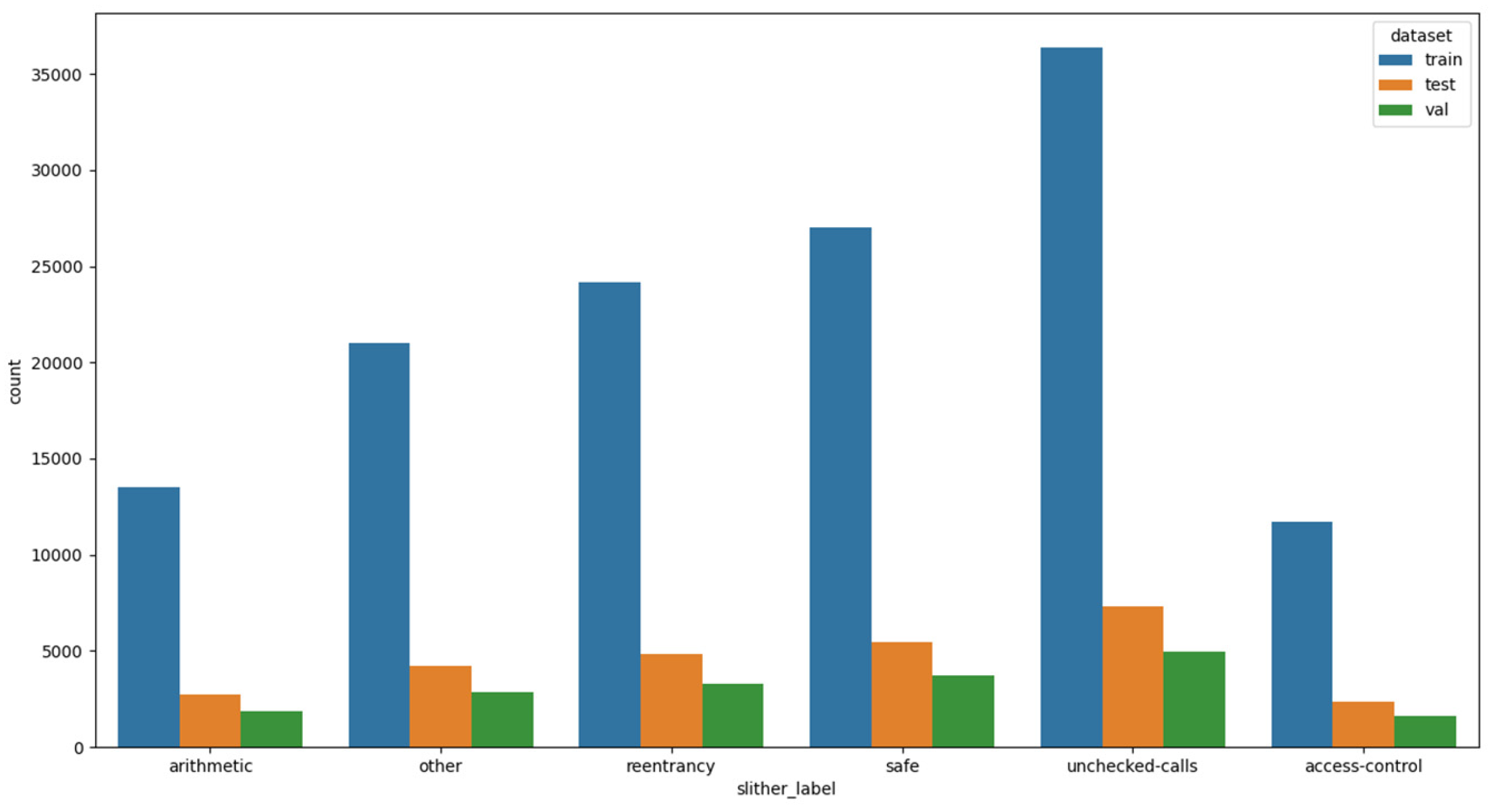
Figure 2.
Part of the CFG for smart contract 0xa840bb63c43e8a428879abe73ddfc7ed0213a96f.
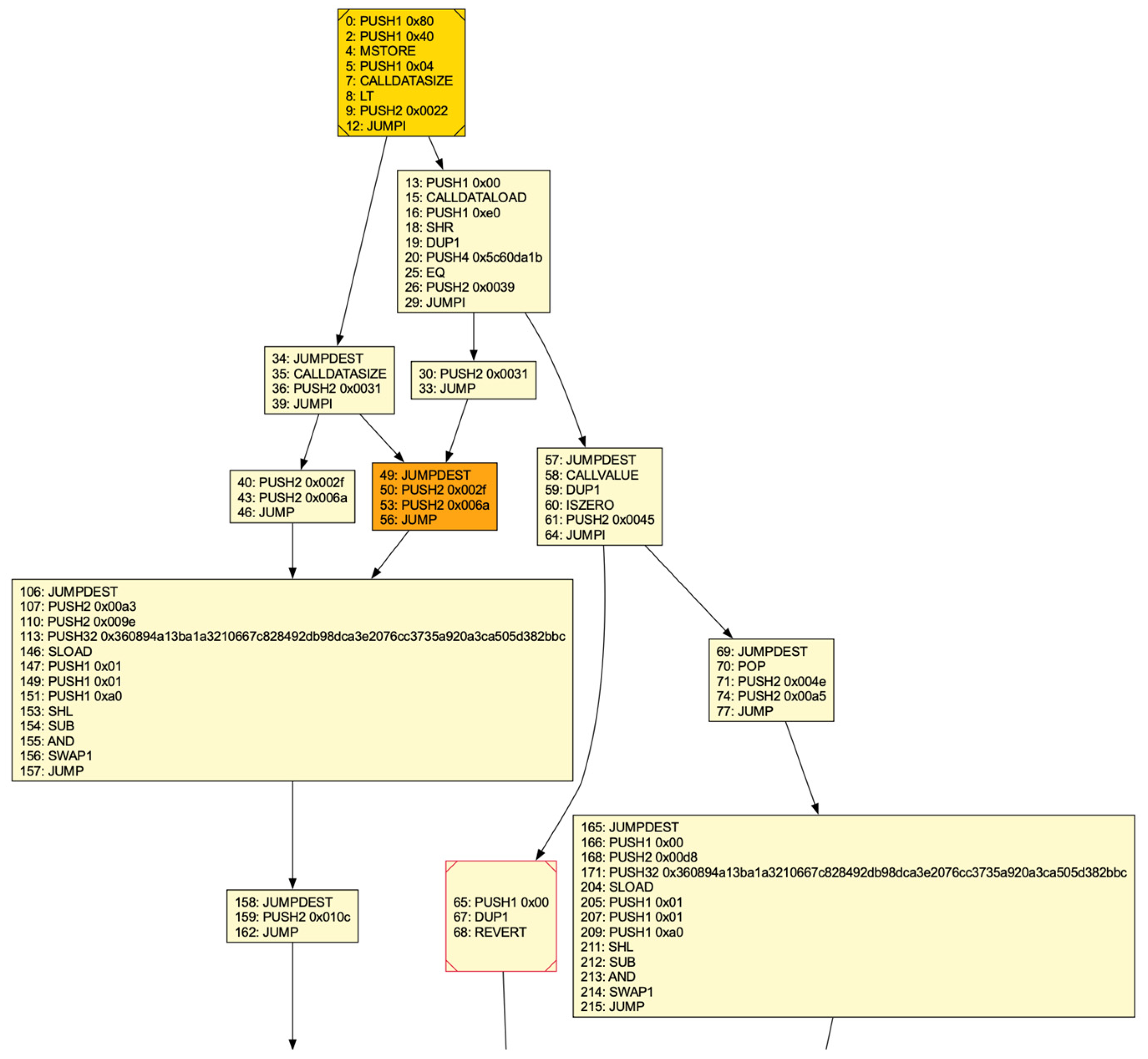
Figure 3.
Model architecture of Q-learning and DQN.
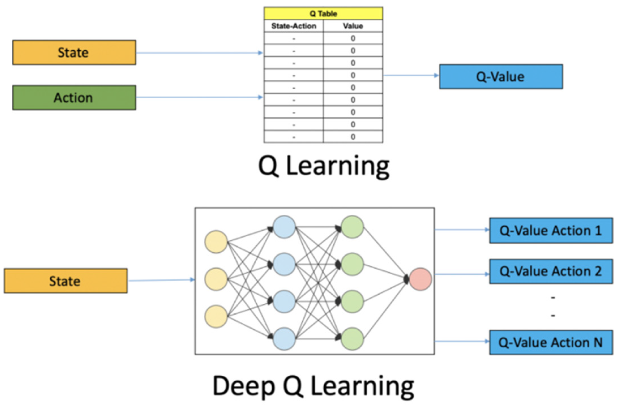
Figure 4.
PPO’s effectiveness across vulnerability categories: (a) ROC curve; (b) PR curve.
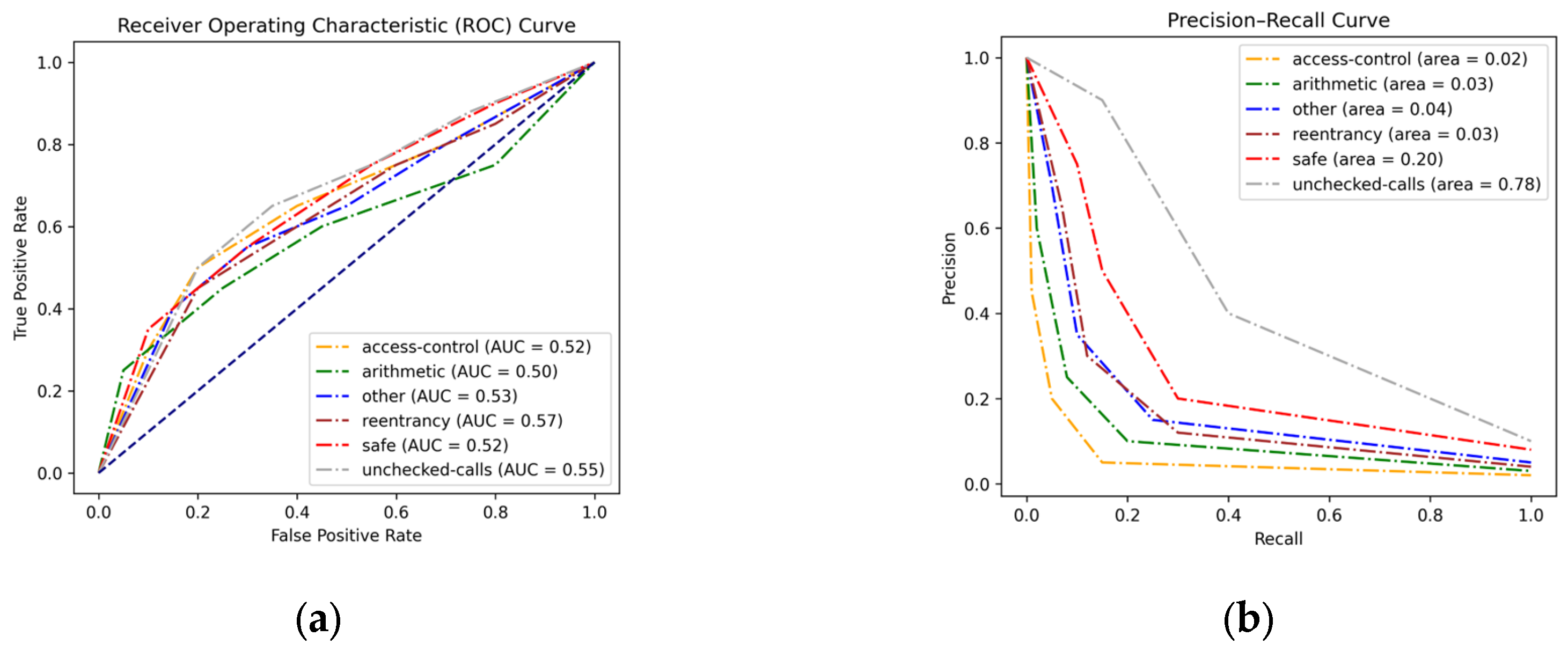

Table 1.
Number of elements per class in the training set.
| Vulnerability | Contracts |
|---|---|
| unchecked-calls | 36,770 |
| safe | 26,280 |
| reentrancy | 24,120 |
| other | 20,650 |
| arithmetic | 14,140 |
| access-control | 11,820 |
Table 2.
Hyperparameter tuning for DQN.
| Parameters | Tuning Range | Optimal Results |
|---|---|---|
| Learning rate | [1e-5, 1e-3] | 0.00015 |
| Batch size | < 32, 64, 128> | 64 |
| Gamma | [0.9, 0.9999] | 0.9400 |
| Steps before learning | [1000, 10000] | 3738 |
| Buffer size | [50000, 1000000] | 86245 |
| Max rewards achieved | 551.0 |
Table 3.
Hyperparameter tuning for PPO.
| Parameters | Tuning Range | Optimal Results |
|---|---|---|
| Learning rate | [1e-5, 1e-3] | 0.0002 |
| Batch size | < 32, 64, 128> | 32 |
| Gamma | [0.9, 0.9999] | 0.9543 |
| Number of steps | <64, 128, 256, 512> | 256 |
| Number of epochs | [1, 10] (int) | 9 |
| Entropy coefficient | [1e-8, 1e-2] | 1.3426 |
| Clip range | [0.1, 0.4] | 0.2195 |
| Max rewards achieved | 584.0 |
Table 4.
Comparison of DQN and PPO performance.
| Model | DQN | PPO |
|---|---|---|
| Accuracy | 0.1869 | 0.2947 |
| Recall | 0.1768 | 0.1930 |
| F1 score | 0.1452 | 0.1463 |
Abbreviations: DQN, Deep Q-Network; PPO, Proximal Policy Optimization.
Table 5.
Classification report of PPO model on the test set.
| Precision | Recall | F1-score | Support | |
|---|---|---|---|---|
| access-control | 0.03 | 0.01 | 0.01 | 193 |
| arithmetic | 0.11 | 0.02 | 0.04 | 249 |
| other | 0.15 | 0.03 | 0.05 | 410 |
| reentrancy | 0.25 | 0.03 | 0.05 | 441 |
| safe | 0.21 | 0.17 | 0.19 | 565 |
| unchecked-calls | 0.28 | 0.81 | 0.46 | 693 |
| accuracy | 0.30 | 2534 | ||
| micro avg | 0.19 | 0.19 | 0.17 | 2534 |
| macro avg | 0.20 | 0.18 | 0.14 | 2534 |
| weighted avg | 0.21 | 0.28 | 0.20 | 2534 |
Disclaimer/Publisher’s Note: The statements, opinions and data contained in all publications are solely those of the individual author(s) and contributor(s) and not of MDPI and/or the editor(s). MDPI and/or the editor(s) disclaim responsibility for any injury to people or property resulting from any ideas, methods, instructions or products referred to in the content. |
© 2025 by the authors. Licensee MDPI, Basel, Switzerland. This article is an open access article distributed under the terms and conditions of the Creative Commons Attribution (CC BY) license (http://creativecommons.org/licenses/by/4.0/).
Copyright: This open access article is published under a Creative Commons CC BY 4.0 license, which permit the free download, distribution, and reuse, provided that the author and preprint are cited in any reuse.


