Submitted:
04 April 2025
Posted:
07 April 2025
You are already at the latest version
Abstract
Fault diagnosis in large-scale systems presents significant challenges due to the complexity and high dimensionality of data, as well as the scarcity of labeled fault data, which is hard to obtain during the practical operation process. This paper proposes a novel approach, called Multi-Variable Meta-Transformer(MVMT) to tackle these challenges. In order to deal with the multivariable time-series data, we modify the transformer model, which is the currently most popular model on feature extraction of time series. To enable the transformer model to simultaneously receive continuous and state inputs, we introduced feature layers before the encoder to better integrate the characteristics of both continuous and state variables. Then we adopt the modified model as the base model for meta-learning. More specifically, the Model-Agnostic Meta-Learning (MAML) strategy. The proposed method leverages the power of transformers for handling multi-variable time series data and employs meta-learning to enable few-shot learning capabilities. The case studies conducted on the Tennessee Eastman Process database and a power-supply system database demonstrate the exceptional performance of fault diagnosis in few-shot scenarios, whether based on continuous-only data or a combination of continuous and state variables.
Keywords:
fault diagnosis
; few-shot learning
; time-series data
; meta-learning
; transformer
1. Introduction
Large-scale systems, such as industrial machinery, power grids, and transportation networks, are fundamental to modern infrastructure. Ensuring their dependability and safety requires precise and timely fault detection and diagnosis (FDD). Traditional knowledge-driven fault diagnosis methods rely heavily on extensive mechanistic knowledge and expert experience. However, as system complexity increases, constructing a diagnostic model solely based on first principles becomes infeasible. Consequently, since the early 21st century, FDD in large-scale systems has transitioned into the data-driven era.
With the continuous advancement of deep learning, its application in FDD has garnered significant attention. Deep neural networks excel at extracting features, allowing for precise modeling of complex nonlinear relationships in large-scale systems. However, as network size grows, so does the demand for vast amounts of labeled data. Conventional deep learning-based fault diagnosis methods often require substantial labeled datasets, which are challenging to obtain in real-world scenarios. Moreover, the intricate interconnections and high dimensionality of variables in these systems further complicate the diagnostic process.
One of the key challenges in data-driven FDD is the limited availability of fault samples for each specific fault category. To address this issue, meta-learning has emerged as a promising approach. Meta-learning, or "learning to learn" [1], enables models to generalize from a few examples, making it particularly suitable for fault diagnosis in large-scale systems where labeled data is scarce. It involves deriving prior knowledge from numerous similar few-shot fault diagnosis tasks and utilizing this prior knowledge to build a model that quickly adapts to new fault scenarios. Depending on the type of prior knowledge, meta-learning can be classified into initialization-based, metric-based, and optimizer-based methods.
Among these, Model-Agnostic Meta-Learning (MAML) is one of the most effective initialization-based approaches. MAML learns an optimal set of initial network weights from a large number of source domain samples, which serves as prior knowledge [2]. This knowledge is then applied to the target domain, enabling rapid adaptation for few-shot fault diagnosis tasks. Initially, MAML was implemented using Convolutional Neural Networks (CNN), which are well-suited for feature extraction from 2D image data. However, when analyzing multivariate time-series data in complex systems, CNNs may fall short due to their limited ability to capture temporal dependencies.
While MAML is designed to work with different parameterized models, integrating Recurrent Neural Networks (RNNs) or Long Short-Term Memory (LSTM) networks—commonly used for time-series analysis—poses computational challenges. The recurrent nature of these architectures requires extensive computations and backpropagation, significantly slowing down the meta-training process. As a result, traditional recurrent architectures, despite their effectiveness in multivariate time-series classification, are not well-suited for MAML-based FDD.
To overcome these limitations, recent advancements in deep learning have introduced Transformers, which have demonstrated exceptional performance in handling complex, high-dimensional data. Unlike RNNs, Transformers utilize position encoding to retain sequence information without relying on recurrence, making them a compelling choice for meta-learning applications.
In real-world fault diagnosis scenarios, multivariate time-series data often consists of both continuous analog and discrete state variables. To effectively capture the unique characteristics of these variable types, we propose an enhanced Transformer model. In our approach, analog and state variables are processed through separate embedding layers to extract their respective feature representations before being fed into the Transformer’s encoder for multi-head self-attention operations. This architecture ensures that both types of variables are effectively merged and utilized for fault diagnosis.
By integrating this enhanced multi-variable Transformer model with MAML, we introduce the Multi-Variable Meta-Transformer (MVMT), a novel approach specifically designed for small-sample fault diagnosis in large-scale systems. Unlike existing methods, MVMT effectively captures the unique characteristics of both continuous analog and discrete state variables through separate embedding layers, ensuring a more comprehensive representation of multivariate time-series data. Furthermore, by leveraging the self-attention mechanism of Transformers, our approach overcomes the limitations of recurrent structures, significantly improving both computational efficiency and adaptation speed in meta-learning.
To rigorously evaluate the effectiveness of MVMT, we conducted extensive experiments on the Tennessee Eastman Process (TEP) dataset and a satellite power-supply system dataset. Comparative analysis with state-of-the-art neural networks, including LSTM, CNN, and Vision Transformer (ViT) combined with meta-learning, demonstrates that MVMT achieves superior fault diagnosis accuracy while maintaining high training efficiency. This work makes three key contributions: (1) introducing a Transformer-based meta-learning framework tailored for multivariate time-series fault diagnosis in the few-shot scenario, (2) proposing a novel embedding mechanism that effectively integrates both analog and state variables, and (3) validating the effectiveness of MVMT through comprehensive experimental comparisons on benchmark and real-world datasets. Our findings underscore the potential of Transformer-based meta-learning in addressing the challenges of few-shot fault diagnosis in complex large-scale systems.
The article will progress as follows: Chapter 2 will discuss related work, focusing on the use of transformers in fault diagnosis and advancements in meta-learning for addressing fault diagnosis with limited data. Chapter 3, Methodology, will detail the MVMT method, outlining its model structure and training approaches. Chapter 4 will cover the experimental setup, detailing the datasets used and the experimental configurations. Chapter 5 will showcase the experimental results and offer a detailed analysis. Finally, Chapter 6 will present conclusions regarding the MVMT method.
2. Related Work
Fault diagnosis in large-scale systems has evolved significantly over the years, with recent advancements in deep learning, particularly transformers, and meta-learning techniques addressing key challenges such as high-dimensional data and limited labeled examples.
2.1. Transformers in Fault Diagnosis
The self-attention deep network Transformer was originally proposed for natural language processing tasks [3]. Due to its self-attention mechanism, Transformer has demonstrated excellent capabilities in handling sequential data. This mechanism enables Transformer to capture long-term temporal dependencies and complex features, making it intuitively well-suited for time series data analysis. In the context of fault diagnosis, Transformer has shown great potential in extracting features from long-term sequential data.
In recent years, Transformer models have demonstrated significant potential in the field of mechanical equipment fault diagnosis. Jin et al. [4] proposed a rotating machinery fault diagnosis method based on the time series Transformer (TST). This method introduced a new time series tokenizer to convert one-dimensional data into a format suitable for Transformer processing. Experimental results showed that TST achieved higher fault diagnosis accuracy than traditional CNN and RNN models on the CWRU, XJTU-SY, and UCONN datasets. As the first attempt to apply Transformer to the field of mechanical fault diagnosis, it directly tokenizes the time series data, which is an operation that converts time series data into discrete tokens, and then feeds them into the classical Transformer model. The overall structure is shown in Figure 1.
Hou et al. [5] designed a bearing fault diagnosis method based on Transformer and ResNet (TAR). This method first used a one-dimensional convolutional layer to perform feature separation and embedding on the original signal and then passed it to the Transformer encoder and ResNet framework for feature extraction. The application of transfer learning strategies reduced the training difficulty of new tasks. Experimental results on the CWRU dataset showed that TAR achieved a fault diagnosis accuracy of 99.90% under noise-free conditions, and its average fault diagnosis accuracy under different signal-to-noise ratios was also higher than that of comparative methods.
Fang et al. [6] proposed a lightweight Transformer called CLFormer for rotating machinery fault diagnosis. This model replaced the original embedding module with a convolutional embedding module and used a linear self-attention mechanism to reduce model complexity. In experiments, the number of parameters of CLFormer was reduced from 35.22K in the original Transformer to 4.88K, and the fault diagnosis accuracy was improved from 82.68% to 90.53%, demonstrating its practical value.
Hou et al. [7] designed a multi-feature parallel fusion rolling bearing fault diagnosis method based on Transformer, called Diagnosisformer. This method first performed fast Fourier transform on the original vibration data to extract frequency domain features and then extracted local and global features of the data through a multi-feature parallel fusion encoder. Experimental results on self-made rotating machinery fault diagnosis data and the CWRU dataset showed that the average diagnosis accuracy of Diagnosisformer reached 99.84% and 99.85%, respectively, significantly outperforming methods such as CNN, CNN-LSTM, RNN, LSTM, and GRU.
Yang et al. [8] proposed a signal Transformer (SiT) based on an attention mechanism and applied it to bearing fault diagnosis research. This method used short-time Fourier transform to convert one-dimensional fault signals into two-dimensional images, which were then fed into the Transformer model for classification. Experimental results showed that compared with traditional convolutional models, SiT performed better in processing fault time information and improved classification accuracy.
In recent years, Transformer-based fault diagnosis methods have advanced rapidly. Starting from the initial TST model, a series of new methods and technologies have emerged and evolved at a fast pace. However, despite these advancements, the application of Transformer models in fault diagnosis still faces several key limitations:
- Data Scarcity: Although Transformer models excel on large-scale datasets, acquiring sufficient labeled data remains a major challenge in complex system fault diagnosis, particularly in few-shot learning scenarios. In many industrial applications, system failures are rare, leading to a severe shortage of samples for each fault type. Despite its powerful feature extraction capabilities, Transformer typically relies on a vast amount of labeled data for effective training, which is often impractical in real-world settings. While some unsupervised learning methods have been proposed, they still require a large number of unlabeled samples and fail to fundamentally overcome the limitations imposed by sample scarcity on model performance.
- Multivariate Issues: As observed in previous studies, nearly all research relies on publicly available bearing datasets to benchmark against state-of-the-art methods. While this approach intuitively evaluates the performance of proposed methods, bearing datasets inherently consist of single-variable time series data collected from vibration sensors. In contrast, data in complex systems often comprise multivariate time series, making it challenging for bearing datasets to accurately reflect the effectiveness of Transformer-based fault diagnosis methods in more diverse and realistic application scenarios.
- Time Series Nature: Since bearing datasets typically consist of high-frequency sampled time series data, researchers often tokenize or transform them into the frequency domain for processing. However, in large and complex systems—such as process industries and spacecraft—the sampling frequency is usually much lower. Due to limited sampling rates and fewer data points, conventional operations like segmentation or tokenization may fail to effectively extract meaningful features. Consequently, determining how to process these measurement variables and efficiently input them into Transformer models remains an urgent challenge that needs to be addressed.
- State Variables: Similar to the previous issues, bearing datasets primarily collect vibration signals, which are analog data. However, in complex systems, measurement data often include crucial state variables, such as switch states and operating modes, which significantly impact system behavior. Despite their importance, these state variables have not been adequately considered in model inputs. Effectively processing these state variables and seamlessly integrating their features with analog data remains a critical challenge in fault diagnosis.
2.2. Advancements of Meta-Learning in Fault Diagnosis
In recent years, meta-learning has emerged as a promising approach to address challenges in fault diagnosis of complex systems, particularly under conditions of limited data availability and varying operational environments. Traditional deep learning methods often require large amounts of labeled data and may struggle to generalize across different working conditions. Meta-learning, or "learning to learn," aims to enable models to rapidly adapt to new tasks with minimal data by leveraging prior experience from related tasks. Model-Agnostic Meta-Learning (MAML) is a prominent meta-learning approach that has been widely adopted due to its ability to quickly adapt to new tasks with only a few examples. MAML optimizes the model’s initial parameters, enabling rapid fine-tuning for specific tasks, making it particularly well-suited for fault diagnosis scenarios where labeled fault data is scarce.
One notable application of meta-learning in fault diagnosis is the development of the Meta-Learning Fault Diagnosis (MLFD) framework. This approach utilizes MAML to learn initial model parameters that can be quickly fine-tuned to new fault diagnosis tasks with limited data. By converting raw vibration signals into time-frequency images and organizing tasks according to an N-way K-shot protocol, MLFD has demonstrated superior performance in few-shot fault diagnosis scenarios [9].It has shown outstanding performance in bearing fault diagnosis tasks under complex and variable operating conditions. Meanwhile, Chang and Lin [10] introduced an adaptive learning rate and proposed the MLALR method to further enhance fault diagnosis accuracy.
To further enhance adaptability, researchers have combined meta-learning with Neural Architecture Search (NAS). The MetaNAS approach employs meta-learning to find optimal initial parameters, allowing the model to identify the most effective network architecture for new fault modes with only a few gradient updates. This integration addresses the challenge of diagnosing novel fault types under small-sample conditions [11].
Another advancement is the Meta-GENE framework, which focuses on domain generalization in intelligent fault diagnosis. By incorporating gradient aligning and semantic matching strategies within a meta-learning framework, Meta-GENE enhances the model’s ability to generalize across different domains, making it particularly useful in industrial environments with diverse operating conditions [12].
Furthermore, there has been a growing interest in combining meta-learning with transformers to leverage the strengths of both approaches. Transformers, with their powerful feature extraction capabilities, serve as an excellent base model for meta-learning. The integration of transformers with MAML allows for effective handling of multi-variable time-series data and enables fast adaptation to new fault types with limited labeled data. This combination has demonstrated superior performance in few-shot fault diagnosis tasks, offering a robust and scalable solution for large-scale systems.
In summary, the application of transformers in fault diagnosis and the advancements in meta-learning techniques have significantly contributed to addressing the challenges of high-dimensional data and limited labeled examples. The integration of these approaches, as proposed in this work, holds great potential for improving the accuracy, efficiency, and adaptability of fault diagnosis models in complex, large-scale systems.
3. Methodology
3.1. Overall framework of the Multi-Variable Meta-Transformer(MVMT)
By seamlessly integrating MAML, the Transformer model, and multi-variable fusion strategies, we introduce the Multi-Variable Meta-Transformer (MVMT). Designed for high efficiency and accuracy, MVMT enables rapid feature extraction and classification, even when only a few samples of both analog and state variables are available. The overall framework of MVMT is depicted in Figure 2.
The MVMT framework is structured into three key stages:
- Data Collection and Preprocessing: Faults are classified as either source faults or target faults based on the number of available samples. Source faults, being common, have a sufficient number of samples, whereas target faults are rare and have only a limited number of samples. These faults are then allocated to a meta-training task set and a meta-testing task set, respectively. Notably, the faults in the meta-testing set are entirely distinct from those in the meta-training set. Unlike conventional train-test splits, fault types included in the meta-training set do not reappear in the meta-testing set.
- Meta-Training Phase: In this stage, a MAML strategy is employed to train the multi-variable Transformer model, optimizing its initial parameters. This process yields a well-initialized multi-variable Transformer encoder, which serves as the foundation for the subsequent meta-testing phase.
- Meta-Testing Phase: Here, the pre-trained multi-variable Transformer model is fine-tuned using the limited samples of rare faults, enabling it to effectively perform the final few-shot fault diagnosis task.
The following sections provide a detailed explanation of the meta-learning techniques, the Transformer model, and the overall architecture and training process of the MVMT model.
3.2. Meta-Learning Framework
To enhance the few-shot learning capability of the base model, we integrate it into a meta-learning framework, specifically leveraging Model-Agnostic Meta-Learning (MAML). MAML optimizes model parameters to facilitate rapid adaptation to new tasks, even with only a few available data samples.
In the context of few-shot learning for fault diagnosis, each task T consists of N fault types (N-way), with K support samples (K-shot) per type, Q query samples, and a specific loss function .
The core idea of MAML is to determine an optimal model initialization such that, under the distribution of the entire classification task set, a model initialized with can be quickly trained to achieve high performance. In other words, this initialization enables the model to efficiently adapt to various classification tasks within the task set.
The MAML algorithm consists of two key optimization processes: meta-training and meta-testing. During meta-training, the model learns from multiple tasks to enhance its ability to adapt rapidly. The objective is to identify an optimal initial parameter from the source domain dataset during meta-training and transfer it as prior knowledge to the target domain. This allows the model to fine-tune efficiently with only a few gradient updates in the target domain, enabling effective adaptation to new tasks.
Figure 3 illustrates the relationship between the meta-training and meta-testing phases.
The overall process of the MAML algorithm is as follows:
- Sample B tasks from the task distribution . Each task consists of N fault types, with K support samples for task-specific training and Q query samples for task-specific validation.
- For each task , use the support samples to compute the updated parameters through S iterations of inner-loop training:where is the inner-loop learning rate.
- Evaluate the updated model using the query sets from all B tasks. The task-specific loss function is used to compute the overall meta-objective:
- Update the model parameters using the meta-gradient:where is the meta-learning rate (outer-loop learning rate).
Figure 4 illustrates the workflow of the MAML algorithm. Step 2 represents the inner loop of the process, while steps 1 through 4 form the outer loop.
The objective of the outer loop is to optimize the model’s initial parameters through training on multiple tasks. Specifically, the outer loop attempts to find a good initialization parameter that allows the model to quickly adapt to new tasks. The outer loop updates the initialization parameters using the meta-loss from multiple tasks, thereby enhancing the model’s generalization ability.
The inner loop is used for short-term optimization on each task, with the goal of adjusting the model parameters through a few gradient updates based on the task’s data. The optimization process in the inner loop typically uses gradient descent to update the model parameters. For each task , the model is fine-tuned on the task-specific training data during the inner loop.
While the objectives of the outer and inner loops are different, they are interdependent. The inner loop fine-tunes the parameters on each task, enabling the model to rapidly adapt to the task-specific features. Meanwhile, the outer loop optimizes the initial parameters based on the training results from multiple tasks, allowing the initialization to generalize to different tasks. In MAML, the outer and inner loops alternate, progressively enhancing the model’s adaptability through multiple training iterations.

Table 1.
MAML algorithm for classification tasks.
| Algorithm | MAML for Classification |
|---|---|
| Input: | : learning rate for inner updates |
| : learning rate for meta-update | |
| : distribution over tasks | |
| Output: | Model parameters |
| 1: | Initialize model parameters |
| 2: | while not done do |
| 3: | Sample batch of tasks |
| 4: | for all do |
| 5: | Sample K datapoints |
| 6: | Evaluate using |
| 7: | Compute adapted parameters with gradient descent: |
| 8: | end for |
| 9: | Sample new datapoints |
| 10: | Compute meta-objective: |
| 11: | end while |
During meta-testing, the model uses the learned initial parameters to quickly adapt to new tasks with a few gradient steps, enabling effective few-shot learning.
Meta-SGD is an extension of MAML that not only learns the initial parameters but also learns the learning rates for each parameter during the meta-training process. This provides an additional layer of flexibility and can lead to faster convergence and better performance.
The main modification in Meta-SGD is that each parameter has an associated learning rate . During the meta-training phase, both the initial parameters and the learning rates are updated.
Table 2.
Meta-SGD algorithm for classification tasks.
| Algorithm | Meta-SGD for Classification |
|---|---|
| Input: | : learning rates for inner updates (learned) |
| : learning rate for meta-update | |
| : distribution over tasks | |
| Output: | Model parameters and learning rates |
| 1: | Initialize model parameters and learning rates |
| 2: | while not done do |
| 3: | Sample batch of tasks |
| 4: | for all do |
| 5: | Sample K datapoints |
| 6: | Evaluate using |
| 7: | Compute adapted parameters with learned |
| gradient descent: | |
| 8: | end for |
| 9: | Sample new datapoints |
| 10: | Compute meta-objective: |
| 11: | end while |
During meta-testing, the model uses the learned initial parameters and learning rates to quickly adapt to new tasks with a few gradient steps, enhancing the effectiveness of few-shot learning.
In practical fault diagnosis applications, the number of fault categories in tasks from the source domain may not necessarily match those in the target domain. To address this issue, we introduced an Adaptive Classifier. While traditional MAML uses a fixed classification head, the Adaptive Classifier generates a specific classifier for each task, enabling dynamic adaptation to the number of categories in different tasks.
Table 3.
MAML Algorithm with Adaptive Classifier.
| Step | Description |
|---|---|
| Input | : Inner-loop learning rate |
| : Meta-learning rate | |
| : Task distribution | |
| Output | Optimized model parameters |
| 1: | Initialize model parameters |
| 2: | while not converged do |
| 3: | Sample a batch of tasks from task distribution |
| 4: | for each task do |
| 5: | Sample support set and query set |
| 6: | Construct the adaptive classifier using |
| 7: | Compute task-specific loss: |
| 8: | Compute task-specific parameter updates: |
| 9: | end for |
| 10: | Compute meta-loss on the query set: |
| 11: | Update meta-parameters: |
| 12: | end while |
3.3. Multi-Variable Transformer
The Transformer[3], a deep network based on self-attention, was initially proposed for natural language processing tasks and has demonstrated exceptional capability in capturing long-range dependencies. In this study, we extend the Transformer model to multi-variable time series data, which is prevalent in complex systems such as process industries, energy systems, and on-orbit spacecraft.
3.3.1. Overall Structure of Transformer
The overall architecture of the Transformer, as shown in Figure 5, consists of two main components: the Encoder and the Decoder. The encoder extracts high-level features from the input data, while the decoder utilizes these features to generate predictions.
The encoder consists of N identical layers, each comprising two key components:
1. Multi-Head Self-Attention Mechanism
2. Feed-Forward Network (FFN)
Given an input time series , it is first processed through an Embedding Layer and Positional Encoding before being fed into the Transformer encoder:
The encoder computes representations as follows:
where:
- is the representation at layer l.
- Multi-head attention allows the model to learn various time dependencies.
- The Feed-Forward Network (FFN) applies nonlinear transformations to enhance feature representations.
The decoder has a similar structure but includes an additional Cross-Attention layer to incorporate information from the encoder output. The decoder computation follows:
where:
- is the decoder representation at layer l.
- The cross-attention mechanism allows the decoder to access encoder representations , improving prediction performance.
The decoder’s final output is passed through a linear layer followed by a Softmax function to obtain the final prediction:
where:
- and are learnable parameters.
- For classification tasks, Softmax outputs a probability distribution over classes.
- For regression tasks, the model directly outputs the predicted values.
Multi-Head Self-Attention is a crucial component of the Transformer model, enabling it to dynamically assign varying levels of importance to different variables. The self-attention mechanism is formulated as follows:
3.3.2. Self-Attention Mechanism
The core of the Transformer model is the self-attention mechanism, which dynamically weighs the importance of different time steps and variables, thereby improving feature representation. The standard scaled dot-product attention mechanism is defined as:
where:
- Q (Query): Represents the current time step information.
- K (Key): Stores information about the entire input sequence.
- V (Value): Stores the feature representations of the input sequence.
- is the dimensionality of the key vectors.
The computation process involves:
1. Computing similarity: Performing the dot product .
2. Scaling: Dividing by to prevent gradient explosion.
3. Softmax normalization: Generating attention weights.
4. Weighted sum: Computing the final attention output.
To enhance feature learning, the Transformer employs multi-head attention, allowing multiple independent attention heads to focus on different aspects of the input:
where:
-h is the number of attention heads.
- Each represents an independent attention mechanism.
- is a learnable linear transformation matrix.
Advantages of multi-head attention:
- Enables the model to capture different levels of features, improving representation capability.
- Avoids local optima that may arise from a single attention head.
3.3.3. Positional Encoding
Since the Transformer lacks inherent recurrence, it explicitly incorporates sequential information via positional encoding, defined as:
where:
- is the position index.
- i is the dimension index.
- is the embedding dimension.
Functionality:
- Ensures temporally close time steps have similar representations.
- Enables the Transformer to recognize sequence order, improving time series modeling.
3.3.4. Multi-Variable Transformer Architecture
Since fault diagnosis is a classification task, we use only the Transformer encoder without the decoder. Given that multi-variable data includes both numerical (analog) and categorical (state) data, we design two separate Transformer encoders for feature extraction. Figure 6 illustrates the multi-variable Transformer structure.
For analog variables, the embedding layer employs a fully connected Feed-Forward Network (FFN), whereas for categorical state variables, we utilize a Word2Vec-based embedding approach. Word2Vec maps discrete state variables into a continuous vector space, allowing them to be processed effectively by the Transformer encoder.
Finally, the outputs from both Transformer encoders are concatenated into a feature matrix (feature size sequence length N) and passed into an adaptive classifier to generate the final classification result.
3.4. Discussion on Time Complexity
During our research, we observed significant variations in computational time when using different types of neural networks as the backbone model for MAML, even with the same parameter scale. In fault diagnosis practices, if conditions permit, longer input sequences are often preferred to achieve higher diagnostic accuracy. Therefore, this section discusses the time complexity of MAML when LSTM, 1D CNN, and Transformer are used as the backbone models concerning the input sequence length N.
LSTM (Long Short-Term Memory) has a computational complexity of per time step, where d represents the hidden layer dimension. Therefore, for a sequence of length N, the total computational complexity of LSTM is .
For a 1D Convolutional Neural Network (1D CNN), the computational complexity is primarily determined by the convolution operations. Assuming the input sequence length is N, the convolution kernel size is k, and the output dimension of the convolution layer is d (i.e., the number of channels), the computational complexity of the convolution operation is .
The computational complexity of a Transformer model is mainly attributed to the self-attention mechanism. The self-attention operation at each position involves pairwise interactions, leading to a complexity of . Considering the feature dimension d, the computational complexity per layer is , resulting in an overall complexity of .
In MAML, gradient computation requires two forward passes and one backward pass. Therefore, the time complexity for different models combined with MAML is:
From a theoretical perspective, the influence of sequence length N is most significant for the Transformer + MAML approach. This implies that the computational cost of MVMT increases with longer sequences. However, in practical experiments, we observed that when the sequence length is relatively short, the absolute training time of a Transformer with the same scale is comparable to that of LSTM, while CNN remains the fastest. As the sequence length increases, the computational burden of LSTM rises more sharply than that of the Transformer, whereas the computational time of the Transformer and CNN increases at a slower rate. This discrepancy between theoretical complexity and actual runtime can be attributed to GPU parallelism.
- 1D CNN: Convolution operations exhibit high parallelism, especially on GPU, allowing for more efficient acceleration compared to LSTM and Transformer models. This advantage is particularly evident when processing long sequences and large batches.
- LSTM: While LSTM can leverage GPU for batch computations, its inherently sequential nature limits parallel efficiency. Since each time step must be computed before the next one begins, LSTM computations remain fundamentally serial, resulting in a complexity of even on GPU.
- Transformer: Owing to its fully parallelizable self-attention mechanism, Transformer models benefit significantly from GPU acceleration. Since attention computations at each position are independent, Transformers generally outperform LSTMs in terms of efficiency, particularly as sequence length N increases.
In conclusion, although Transformer models theoretically have higher computational complexity, GPU acceleration significantly mitigates their runtime cost in practice. Compared to LSTM, the Transformer becomes increasingly advantageous as the sequence length grows. Moreover, since MAML involves both inner-loop and outer-loop updates, the integration of the MAML algorithm further enhances the training efficiency of the Transformer model.
4. Experimental Setup
4.1. Datasets
We evaluate our approach on two datasets: Tennessee Eastman Process (TEP) Dataset and Power-Supply System Dataset
4.1.1. Dataset 1: TEP
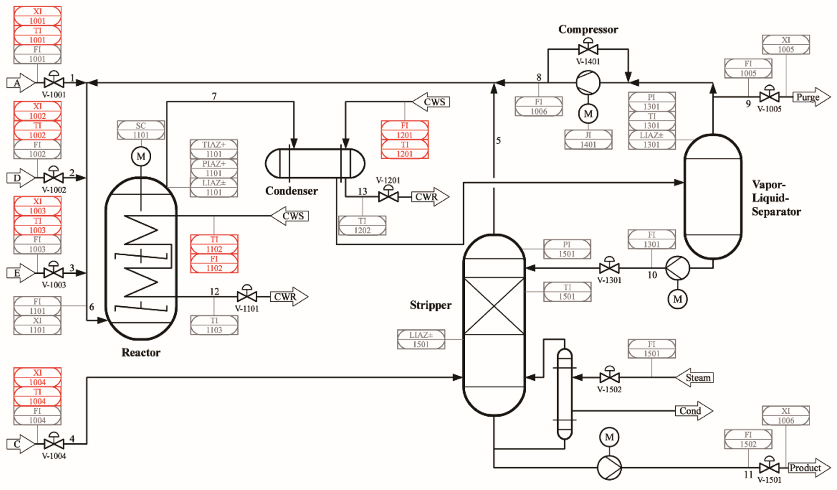
The Tennessee-Eastman (TE) process is a well-established chemical process simulation system that represents a typical industrial chemical production process involving multiple unit operations and a set of adjustable variables. It simulates a large-scale chemical plant, with its core centered around an ethylene production process. Through precise modeling and simulation, the TE process captures common dynamic and nonlinear behaviors in chemical operations, including improper control actions, process faults, and other operational anomalies. It is widely utilized in research on process control, optimization, monitoring, and fault diagnosis. The TE dataset encompasses 20 typical fault modes observed in industrial processes, making it a standard benchmark for process monitoring and fault diagnosis studies. Further details can be found in Appendix Table A1.
Figure 7.
Tennessee-Eastman process schematic diagram.
The TE process dataset consists of multiple subsets, with each fault mode containing both a training set and a testing set. The dataset size is as follows:
- Training Set: The training set for each fault mode contains 480 samples.
- Testing Set: The testing set for each fault mode contains 960 samples.
Each data sample contains 53 variables, including:
- 40 Process Variables
- 13 Manipulated Variables
A complete list of all variables is provided in Appendix Table A2.
Considering that different fault types vary in detection difficulty, we allocated fault types with similar difficulty levels between the meta-training set and the meta-testing set based on diagnostic accuracy under sufficient sample conditions.
Table 4.
TEP Dataset: Fault Types in Meta-Training and Meta-Testing Sets.
| Task Set | Selected Fault Types |
|---|---|
| Meta-Training Set | 3, 5, 6, 7, 8, 9, 10, 11, 15, 16, 18, 19, 20 |
| Meta-Testing Set | 1, 2, 4, 12, 13, 14, 17 |
After dividing the fault types into meta-training and meta-testing sets, we construct two types of few-shot learning tasks:
- Task 1: Each task contains 5 fault types. In the meta-training set, each fault type includes 1 support sample and 5 query samples, whereas in the meta-testing set, each fault type includes 1 support sample and 30 query samples. The length of each sample is 50.
- Task 2: Each task contains 5 fault types. In the meta-training set, each fault type includes 3 support samples and 10 query samples, whereas in the meta-testing set, each fault type includes 3 support samples and 30 query samples. The length of each sample is 30.
The task construction details are summarized in Table 5.
4.1.2. Dataset 2: Power-Supply System
This dataset comprises operational data from a real-world power-supply system of in-orbit spacecraft, including variables related to voltage, current, temperature, and other relevant parameters. It includes labeled instances of different fault conditions that occur in the system.
The dataset contains 24 types of faults, as listed in Appendix Table A3.
Since the number of samples varies across different faults, we divide them into meta-training and meta-testing sets based on actual sample availability. The selected fault types for each set are listed in Table 6.
Based on the division of fault types, we construct three types of few-shot learning tasks:
- Task Setting 1: Each task in both the meta-training and meta-testing sets contains 5 fault types. The meta-training set includes 5 support samples and 10 query samples per task, while the meta-testing set includes 5 support samples and 30 query samples per task. The length of each sample is 30.
- Task Setting 2: The meta-training set contains 5 fault types per task, whereas the meta-testing set contains 7 fault types per task. In the meta-training set, each task consists of 5 support samples and 10 query samples, while in the meta-testing set, each task consists of 5 support samples and 30 query samples. The length of each sample is 30.
- Task Setting 3: Each task in both the meta-training and meta-testing sets contains 5 fault types. The meta-training set includes 3 support samples and 10 query samples per task, while the meta-testing set includes 3 support samples and 30 query samples per task. The length of each sample is 50.
The details of task construction are summarized in Table 7.
4.2. Evaluation Metrics
The evaluation metrics are categorized into two dimensions: efficiency and performance.
For the efficiency dimension, we adopt the total meta-training time, denoted as , as the evaluation metric.
For the performance dimension, we measure the classification accuracy of the trained model (with optimal initialization) on the query samples of all tasks in the test set.
4.3. Comparison Methods
To evaluate the effectiveness of the proposed method, we compare it against the following state-of-the-art meta-learning-based fault diagnosis approaches:
Furthermore, in Dataset 2, we incorporate the meta-SGD strategy to explore its impact on both efficiency and performance across different models.
4.4. Hyperparameter Settings
To ensure a rigorous and fair comparison, we conducted preliminary experiments using a sufficient number of samples from both Dataset 1 and Dataset 2. Each base model was optimized using Optuna, and the final tuned hyperparameters are presented in Table 8 and Table 9.
It is noteworthy that Dataset 2 contains both continuous (analog) and discrete (state) variables. Hence, the input feature size is configured to accommodate both data types.
5. Results and Discussion
5.1. Experimental Results on Dataset 1 (TEP)
Table 10 presents the results of training and testing directly on the meta-test task set without employing the MAML learning strategy. Here, MVT refers to Multi Variable Transformer, which can handle multivariate time series but does not utilize the MAML learning method for training on the meta-test task set from scratch.
Table 11 summarizes the training time and classification accuracy of models incorporating the MAML strategy.
From the results, it is evident that the proposed MVMT model consistently achieves the highest accuracy across both task settings while requiring only half the training time of LSTM+MAML. Although 1DCNN+MAML exhibits the fastest training speed, significantly outperforming other methods in terms of efficiency, its final performance remains inferior to Transformer-based models and is comparable to LSTM. On the other hand, LSTM attains moderate accuracy but incurs the longest training time. Overall, these findings indicate that MVMT offers a clear and consistent advantage in few-shot fault diagnosis tasks for chemical processes.
Moreover, regardless of the model architecture, incorporating the MAML strategy enables the models to learn better initial parameters from the source domain, facilitating rapid adaptation to new tasks in the target domain.
5.2. Experimental Results on Dataset 2 (Power-Supply System)
Table 12 presents the experimental results on Dataset 2, where both analog and state variables are included. Under these conditions, MVMT demonstrates an even greater advantage.
In Task Setting 1 (5-way 5-shot classification), MVMT achieves the highest fault diagnosis accuracy while maintaining stable and efficient training performance. In contrast, LSTM requires the longest training time but fails to deliver accuracy improvements proportional to its computational cost. It is also noteworthy that the MAML algorithm consistently enhances each model’s adaptation to target-domain tasks, as parameters learned from the source domain significantly improve accuracy over random initialization.
When meta-SGD is introduced, the accuracy of 1DCNN and LSTM improves, while training time remains stable or even decreases slightly—likely due to hardware performance fluctuations. However, for Transformer-based models, the application of meta-SGD does not yield significant accuracy gains. In fact, for ViT, accuracy decreases from 78.40% to 72.66%, making it even less effective than LSTM+meta-SGD.
In Task Setting 2, the meta-test tasks involve 7-way classification to evaluate whether the adaptive classifier can handle varying class numbers. The results indicate that the classifier successfully adapts to this scenario, with MVMT again achieving the highest accuracy (73.00%). Although 1DCNN maintains a training time advantage, its accuracy drops significantly compared to Task Setting 1, suggesting that its combination with the adaptive classifier is less effective than MVMT. Regarding the impact of meta-SGD, there is a slight accuracy improvement for 1DCNN and ViT, while its effect on MVMT and LSTM is negligible. Additionally, in the baseline models without MAML, MVT achieves an accuracy close to that of MAML-enhanced 1DCNN, highlighting MVT’s inherent adaptability to different tasks.
Task Setting 3 involves longer sequences but fewer support samples (3-shot). Even under these conditions, MVMT remains the best-performing model, significantly outperforming others. When meta-SGD is introduced, 1DCNN and LSTM show notable accuracy improvements, whereas Transformer-based models see minimal gains. This observation suggests that Transformer models exhibit similar parameter update patterns during training, reducing the need for meta-SGD to adjust learning rates for individual parameters.
6. Conclusion
This paper investigates fault pattern recognition in complex engineering systems based on meta-learning, specifically focusing on fault diagnosis and classification. The limitations of existing methods are analyzed, and the Transformer model is improved. We propose the Multi-Variable Transformer based on Self-Attention Mechanism (MVMT), which fully leverages the rapid adaptability of meta-learning and the powerful feature extraction ability of Transformer. MVMT efficiently performs multi-variable fault pattern recognition under small sample conditions, showing promising application prospects and theoretical value.
- MVMT has excellent feature extraction capabilities, particularly suited for time-series data. It also takes advantage of GPU’s efficient parallel computation capabilities, avoiding the high computational costs associated with traditional Recurrent Neural Networks (RNN) and Long Short-Term Memory (LSTM) networks.
- MVMT can quickly adapt to new fault tasks with only a small amount of data, which is especially important for fault categories with scarce samples in complex systems.
- MVMT effectively integrates different types of variables (e.g., analog and status variables), providing high flexibility for application in complex systems.
- The introduction of an Adaptive Classifier addresses the issue of varying numbers of categories across tasks, a problem that traditional MAML could not handle.
- Comparative experiments on the TE chemical process dataset and on-orbit spacecraft telemetry dataset have shown that MVMT outperforms existing methods in multi-variable, small-sample fault diagnosis tasks for complex systems.
In the future, as the scale of complex engineering systems continues to expand and the number of system components increases, fault diagnosis tasks will face more complex and diversified challenges. First, how to achieve real-time multi-fault pattern recognition and fault detection in more complex systems will be an important direction for future research. Traditional methods often focus on detecting a single fault mode, but in practical applications, multiple fault modes may occur simultaneously or interact with each other. This requires model designs that can simultaneously recognize and distinguish multiple fault modes in parallel. Therefore, future research can explore Multi-Task Learning (MTL) methods based on deep learning, optimizing multiple fault diagnosis tasks simultaneously to enhance the adaptability of models in complex systems.
Second, with the increasing diversification of fault diagnosis data types and sources, how to effectively handle different types of data (e.g., time-series data, image data, text data, etc.) and achieve cross-modal fusion and analysis will be an important direction for future research. Currently, although Transformer models have demonstrated excellent performance in multi-variable time-series data, further technological innovations are needed when handling more complex data forms. For example, combining Graph Neural Networks (GNN) with Transformer models can better model and optimize global information from the system structure and the relationships between nodes, providing more accurate support for global system fault diagnosis.
Finally, with the improvement of computational power and hardware environments, how to apply advanced fault diagnosis technologies in practical industrial environments and promote the popularization of smart manufacturing and Industrial Internet of Things (IIoT) will also be an important research direction. In this process, the interpretability of models will become particularly important, as practical industrial applications often require a clear understanding of the model’s decision-making process. Future research can focus on enhancing the interpretability and transparency of deep learning models, developing efficient, robust, and easy-to-understand fault diagnosis systems that meet the needs of engineering practice. Through the integration and innovation of these technologies, future complex engineering systems will be able to conduct fault detection and prediction more intelligently, significantly improving system reliability and safety.
Author Contributions
Conceptualization, Li, W. and Yang, F.; methodology, Li, W.; validation, Li, W. and Nie, Y.; resources, Yang, F.; data curation, Li, W. and Nie, Y.; writing—original draft preparation, Li, W.; writing—review and editing, Li, W. and Nie, Y.; supervision, Yang, F.; funding acquisition, Yang, F. All authors have read and agreed to the published version of the manuscript.
Funding
This research was funded by National Natural Science Foundation of China, grant number 61873142.
Data Availability Statement
The data supporting the reported results are available at Github under the following link: https://github.com/YPCJ/MVMT.git.
Acknowledgments
The authors would like to thank China Satellite Network Group Co., Ltd for the data support during the experiments.
Conflicts of Interest
The authors declare no conflicts of interest. The funders had no role in the design of the study; in the collection, analyses, or interpretation of data; in the writing of the manuscript; or in the decision to publish the results.
Appendix A. Datasets Detail
Table A1.
Fault description in TEP Dataset
| Fault | Description |
|---|---|
| IDV(1) | A/C Feed Ratio, B Composition Constant (Stream 4) Step |
| IDV(2) | B Composition, A/C Ratio Constant (Stream 4) Step |
| IDV(3) | D Feed Temperature (Stream 2) Step |
| IDV(4) | Reactor Cooling Water Inlet Temperature Step |
| IDV(5) | Condenser Cooling Water Inlet Temperature Step |
| IDV(6) | A Feed Loss (Stream 1) Step |
| IDV(7) | C Header Pressure Loss - Reduced Availability (Stream 4) Step |
| IDV(8) | A, B, C Feed Composition (Stream 4) Random Variation |
| IDV(9) | D Feed Temperature (Stream 2) Random Variation |
| IDV(10) | C Feed Temperature (Stream 4) Random Variation |
| IDV(11) | Reactor Cooling Water Inlet Temperature Random Variation |
| IDV(12) | Condenser Cooling Water Inlet Temperature Random Variation |
| IDV(13) | Reaction Kinetics Slow Drift |
| IDV(14) | Reactor Cooling Water Valve Sticking |
| IDV(15) | Condenser Cooling Water Valve Sticking |
| IDV(16) | Unknown |
| IDV(17) | Unknown |
| IDV(18) | Unknown |
| IDV(19) | Unknown |
| IDV(20) | Unknown |
Table A2.
Variables in TEP Dataset
| Variable | Description | Variable | Description |
|---|---|---|---|
| XMV(1) | D Feed Flow (stream 2) (Corrected Order) | XMEAS(15) | Stripper Level |
| XMV(2) | E Feed Flow (stream 3) (Corrected Order) | XMEAS(16) | Stripper Pressure |
| XMV(3) | A Feed Flow (stream 1) (Corrected Order) | XMEAS(17) | Stripper Underflow (stream 11) |
| XMV(4) | A and C Feed Flow (stream 4) | XMEAS(18) | Stripper Temperature |
| XMV(5) | Compressor Recycle Valve | XMEAS(19) | Stripper Steam Flow |
| XMV(6) | Purge Valve (stream 9) | XMEAS(20) | Compressor Work |
| XMV(7) | Separator Pot Liquid Flow (stream 10) | XMEAS(21) | Reactor Cooling Water Outlet Temp |
| XMV(8) | Stripper Liquid Product Flow (stream 11) | XMEAS(22) | Separator Cooling Water Outlet Temp |
| XMV(9) | Stripper Steam Valve | XMEAS(23) | Component A |
| XMV(10) | Reactor Cooling Water Flow | XMEAS(24) | Component B |
| XMV(11) | Condenser Cooling Water Flow | XMEAS(25) | Component C |
| XMV(12) | Agitator Speed | XMEAS(26) | Component D |
| XMEAS(1) | A Feed (stream 1) | XMEAS(27) | Component E |
| XMEAS(2) | D Feed (stream 2) | XMEAS(28) | Component F |
| XMEAS(3) | E Feed (stream 3) | XMEAS(29) | Component A |
| XMEAS(4) | A and C Feed (stream 4) | XMEAS(30) | Component B |
| XMEAS(5) | Recycle Flow (stream 8) | XMEAS(31) | Component C |
| XMEAS(6) | Reactor Feed Rate (stream 6) | XMEAS(32) | Component D |
| XMEAS(7) | Reactor Pressure | XMEAS(33) | Component E |
| XMEAS(8) | Reactor Level | XMEAS(34) | Component F |
| XMEAS(9) | Reactor Temperature | XMEAS(35) | Component G |
| XMEAS(10) | Purge Rate (stream 9) | XMEAS(36) | Component H |
| XMEAS(11) | Product Sep Temp | XMEAS(37) | Component D |
| XMEAS(12) | Product Sep Level | XMEAS(38) | Component E |
| XMEAS(13) | Prod Sep Pressure | XMEAS(39) | Component F |
| XMEAS(14) | Prod Sep Underflow (stream 10) | XMEAS(40) | Component G |
| XMEAS(41) | Component H |
Table A3.
Fault Descriptions of Power-Supply System
| Number | Device | Unit | Fault Description |
|---|---|---|---|
| 0 | Power Controller | BCRB Module | Single Drive Transistor Open or Short in MEA Circuit |
| 1 | Power Controller | BCRB Module | Single Operational Amplifier Open or Short in MEA Circuit |
| 2 | Power Controller | BCRB Module | Incorrect Battery Charging Voltage Command |
| 3 | Power Controller | Power Lower Machine | CDM Module Current Telemetry Circuit Fault |
| 4 | Power Controller | Power Lower Machine | POWER Module Bus Current Measurement Circuit Fault |
| 5 | Power Controller | Power Lower Machine | Solar Array Current Measurement Circuit Fault |
| 6 | Power Controller | Power Lower Machine | Communication Fault |
| 7 | Power Controller | Global | Load Short Circuit |
| 8 | Power Controller | Power Module | S3R Circuit Diode Short Circuit |
| 9 | Power Controller | Power Module | S3R Circuit Shunt MOSFET Open Circuit |
| 10 | Power Controller | Power Module | Abnormal S3R Shunt Status |
| 11 | Power Controller | Distribution (Heater) Module | Y Board Heater Incorrectly On |
| 12 | Power Controller | Distribution (Heater) Module | Battery Heater Band Incorrectly Off |
| 13 | Power Controller | Distribution (Heater) Module | Battery Heater Band Incorrectly On |
| 14 | Solar Array | Isolation Diode | Short Circuit |
| 15 | Solar Array | Isolation Diode | Open Circuit |
| 16 | Solar Array | Interconnect Ribbon | Open Circuit |
| 17 | Solar Array | Bus Bar | Solder Joint Open Circuit |
| 18 | Solar Array | Solar Cell | Single Cell Short Circuit |
| 19 | Solar Array | Solar Cell | Single Cell Open Circuit |
| 20 | Solar Array | Solar Cell | Solar Cell Performance Degradation |
| 21 | Solar Array | Solar Wing | Single Subarray Open Circuit |
| 22 | Solar Array | Solar Wing | Single Wing Open Circuit |
| 23 | Solar Array | Solar Wing | Solar Wing Single Subarray Open Circuit |
References
- Hospedales, T.; Antoniou, A.; Micaelli, P.; et al. Meta-learning in neural networks: A survey. IEEE Transactions on Pattern Analysis and Machine Intelligence 2021, 44, 5149–5169. [Google Scholar] [CrossRef] [PubMed]
- Finn, C.; Abbeel, P.; Levine, S. Model-agnostic meta-learning for fast adaptation of deep networks. In Proceedings of the Proc. of the 34th Int’l Conf. on Machine Learning, Vol. 70; 2017; pp. 1126–1135. [Google Scholar]
- Vaswani, A.; Shazeer, N.; Parmar, N.; et al. Attention is all you need. In Proceedings of the Advances in Neural Information Processing Systems, Vol. 30. 2017. [Google Scholar]
- Jin, Y.; Hou, L.; Chen, Y. A time series transformer based method for the rotating machinery fault diagnosis. Neurocomputing 2022, 494, 379–395. [Google Scholar] [CrossRef]
- Hou, S.; Lian, A.; Chu, Y. Bearing fault diagnosis method using the joint feature extraction of Transformer and ResNet. Measurement Science and Technology 2023, 34, 075108. [Google Scholar] [CrossRef]
- Fang, H.; Deng, J.; Bai, Y.; Feng, B.; Li, S.; Shao, S.; Chen, D. CLFormer: A lightweight transformer based on convolutional embedding and linear self-attention with strong robustness for bearing fault diagnosis under limited sample conditions. IEEE Transactions on Instrumentation and Measurement 2021, 71, 1–8. [Google Scholar] [CrossRef]
- Hou, Y.; Wang, J.; Chen, Z.; Ma, J.; Li, T. Diagnosisformer: An efficient rolling bearing fault diagnosis method based on improved Transformer. Engineering Applications of Artificial Intelligence 2023, 124, 106507. [Google Scholar] [CrossRef]
- Yang, Z.; Cen, J.; Liu, X.; Xiong, J.; Chen, H. Research on bearing fault diagnosis method based on transformer neural network. Measurement Science and Technology 2022, 33, 085111. [Google Scholar] [CrossRef]
- Li, C.; Li, S.; Zhang, A.; He, Q.; Liao, Z.; Hu, J. Meta-learning for few-shot bearing fault diagnosis under complex working conditions. Neurocomputing 2021, 439, 197–211. [Google Scholar] [CrossRef]
- Chang, L.; Lin, Y.H. Meta-Learning With Adaptive Learning Rates for Few-Shot Fault Diagnosis. IEEE/ASME Transactions on Mechatronics 2022, 27, 5948–5958. [Google Scholar] [CrossRef]
- Li, X.; Li, X.; Li, S.; Zhou, X.; Jin, L. Small sample-based new modality fault diagnosis based on meta-learning and neural architecture search. Control and Decision 2023, 38, 3175–3183. [Google Scholar]
- Ren, L.; Mo, T.; Cheng, X. Meta-learning based domain generalization framework for fault diagnosis with gradient aligning and semantic matching. IEEE Transactions on Industrial Informatics 2023, 20, 754–764. [Google Scholar] [CrossRef]
- Hochreiter, S.; Schmidhuber, J. Long short-term memory. Neural computation 1997, 9, 1735–1780. [Google Scholar] [CrossRef] [PubMed]
- LeCun, Y.; Bengio, Y. Convolutional networks for images, speech, and time series. In The Handbook of Brain Theory and Neural Networks; 1995; pp. 3361–1995.
- Dosovitskiy, A.; Beyer, L.; Kolesnikov, A.; et al. An image is worth 16x16 words: Transformers for image recognition at scale. In Proceedings of the International Conference on Learning Representations (ICLR); 2021. [Google Scholar]
Figure 1.
Schematic diagram of the Time Series Transformer (TST) structure [4].
Figure 1.
Schematic diagram of the Time Series Transformer (TST) structure [4].
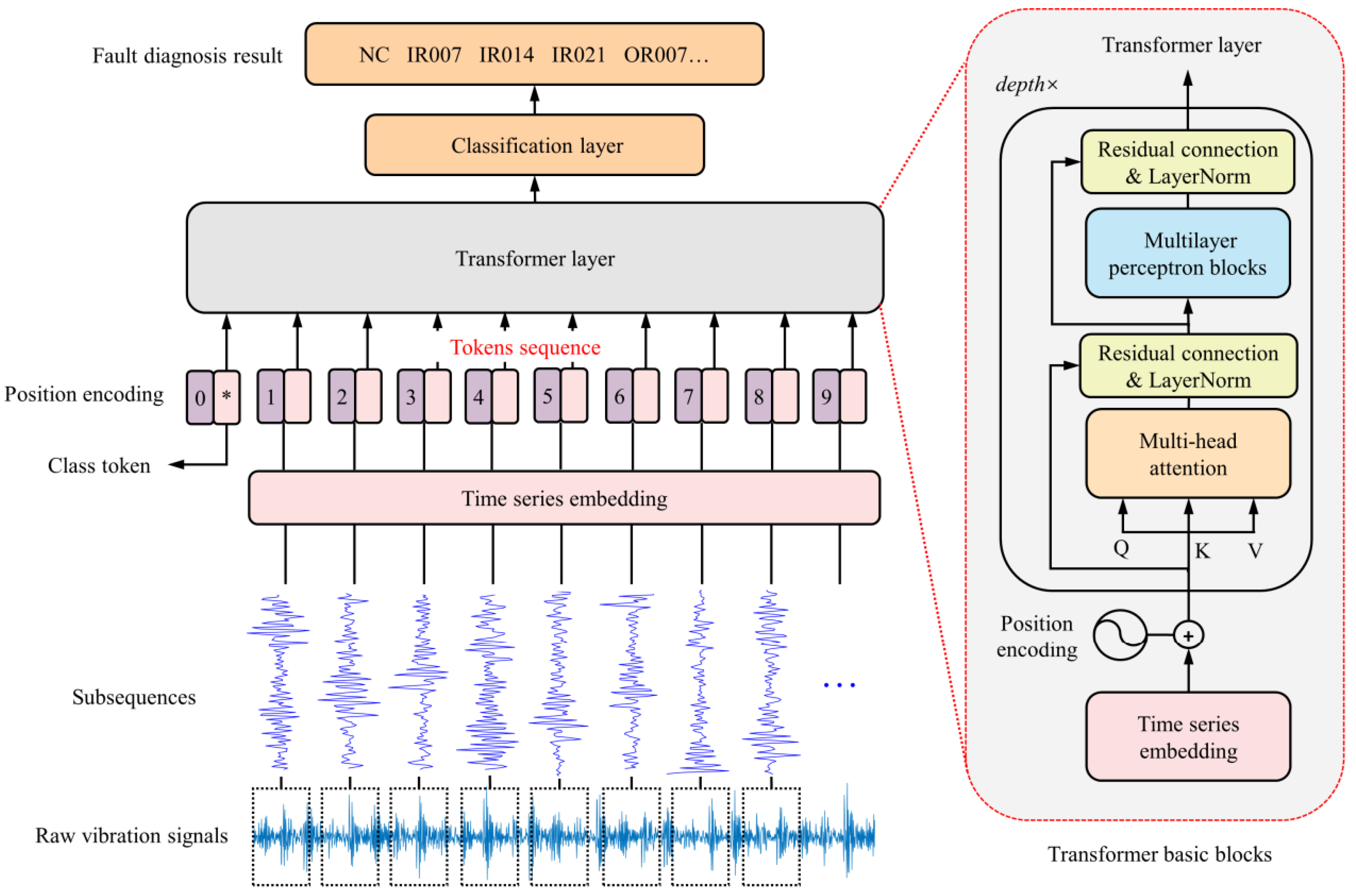
Figure 2.
Overall framework of the Multi-Variable Meta-Transformer.
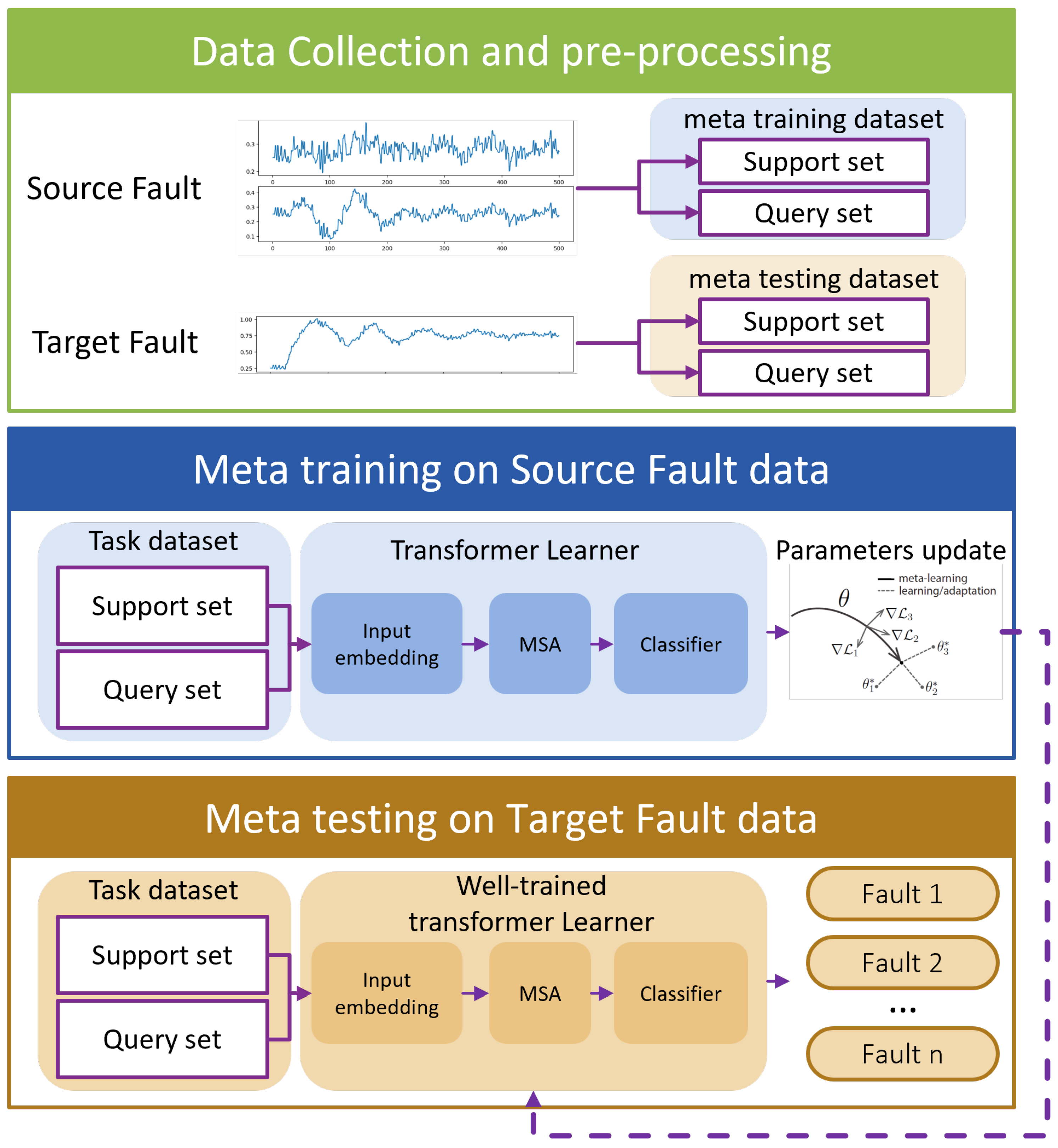
Figure 3.
Relationship between meta-training and meta-testing.
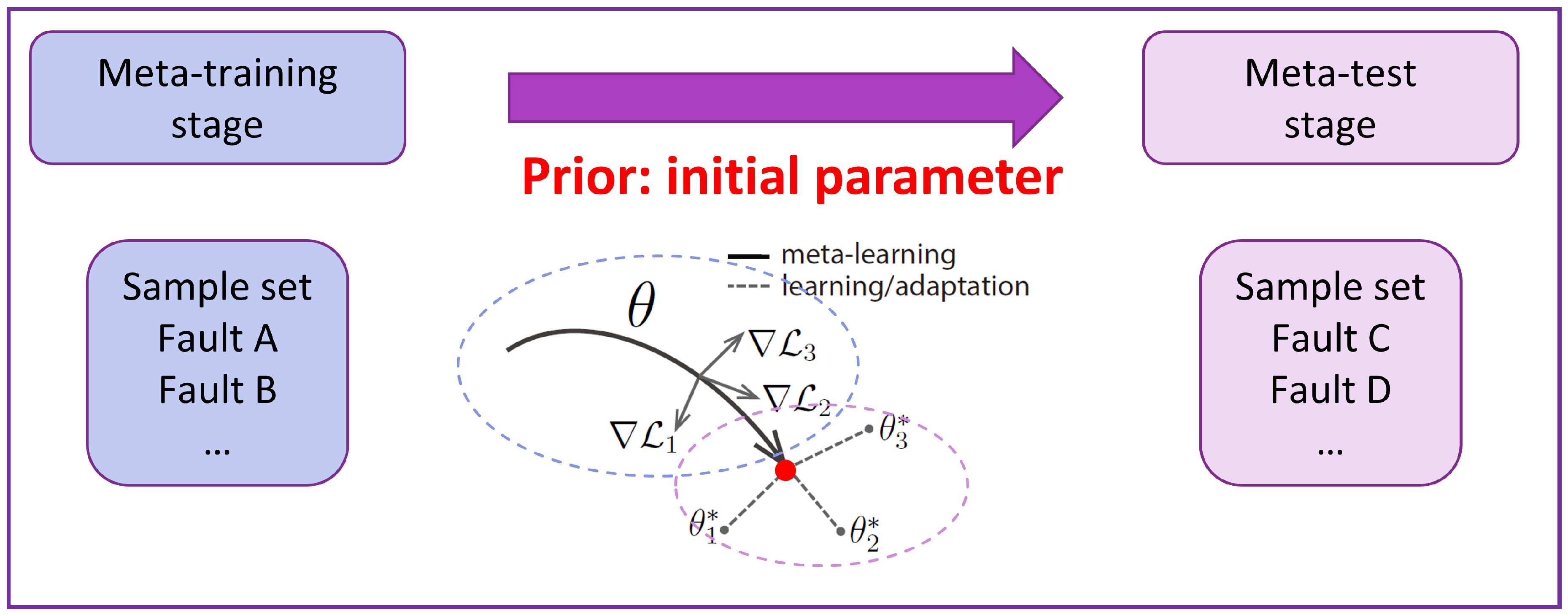
Figure 4.
MAML algorithm workflow.
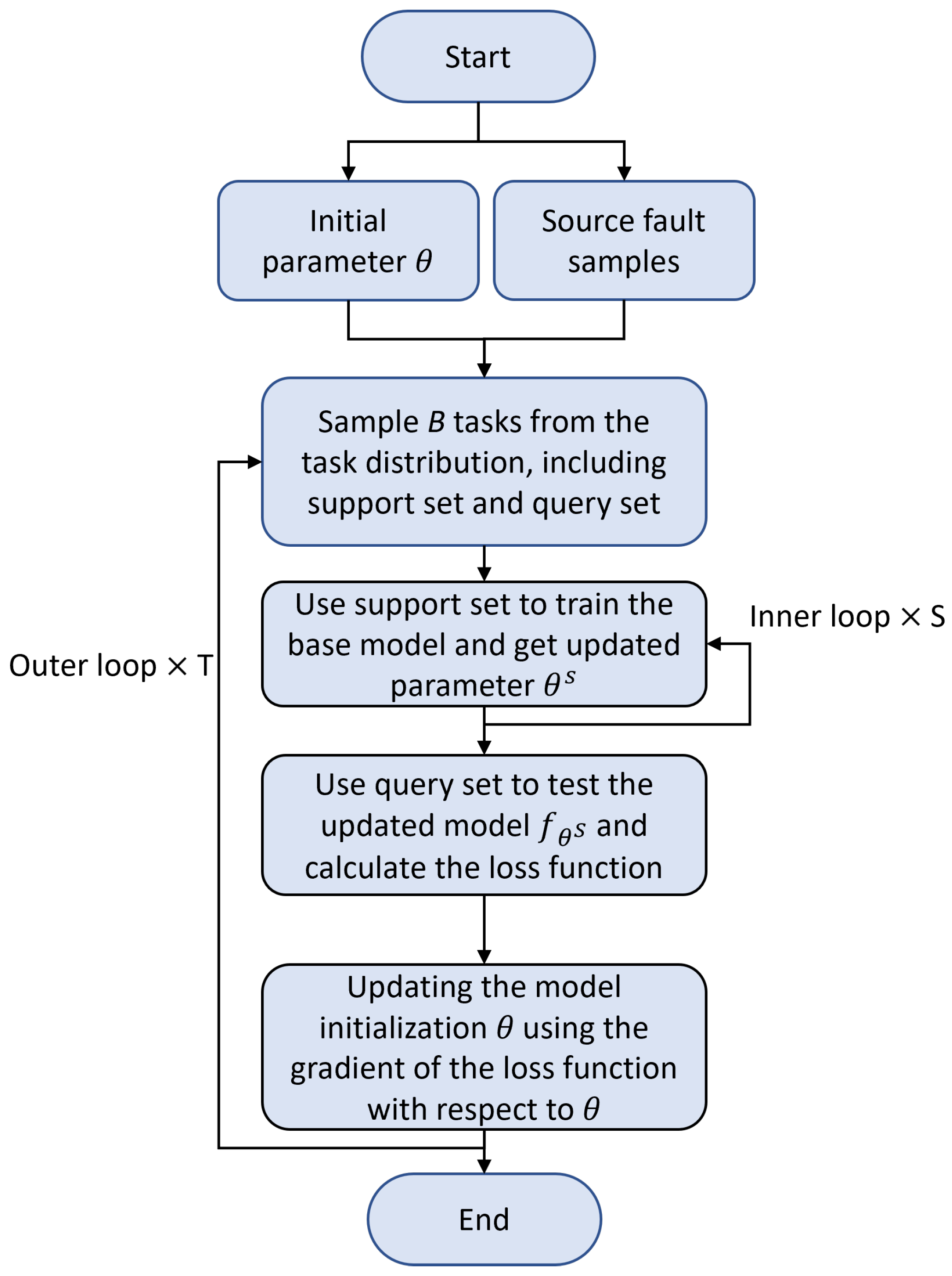
Figure 5.
Transformer Structure includes multiple encoders and decoders [3].
Figure 5.
Transformer Structure includes multiple encoders and decoders [3].
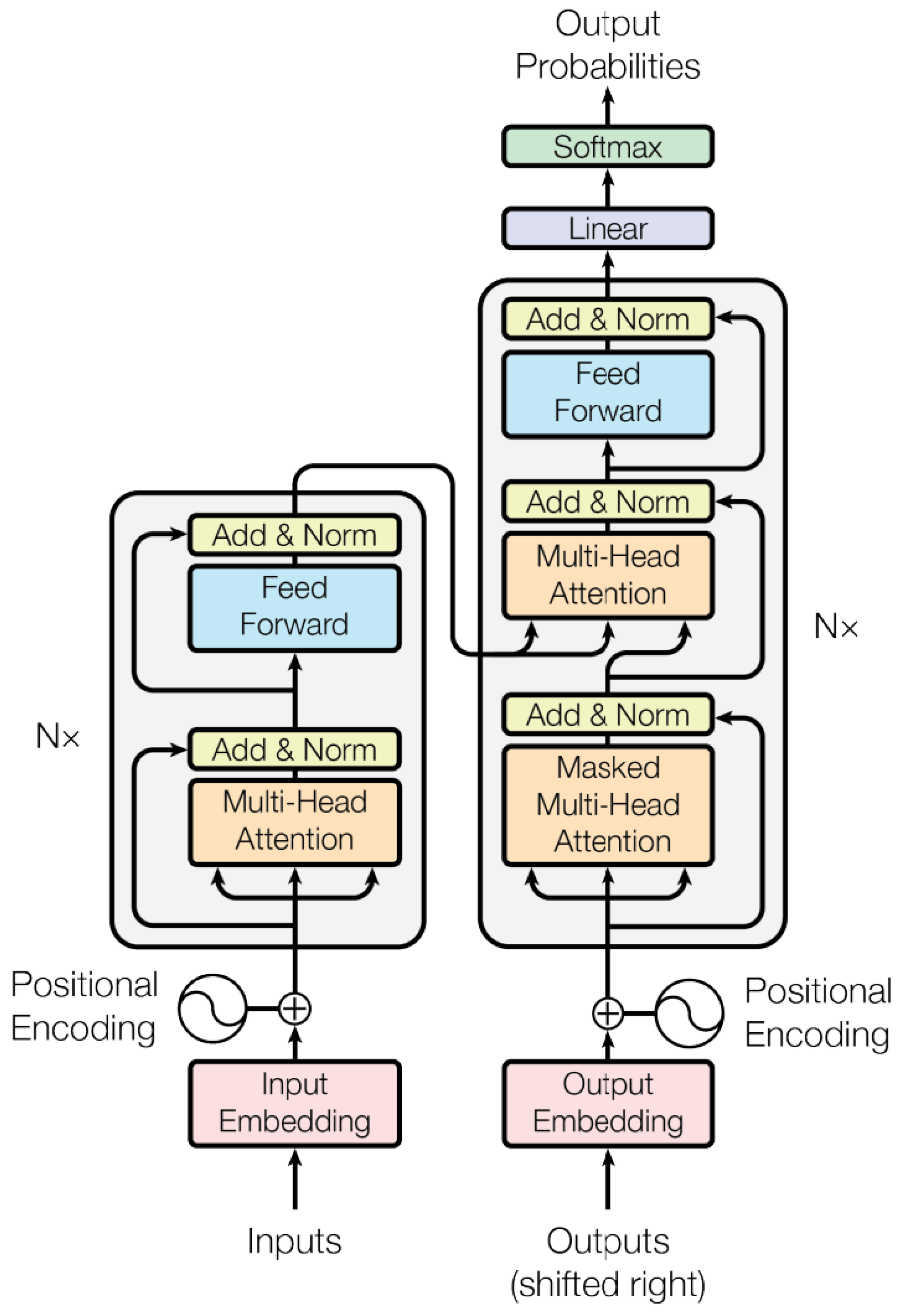
Figure 6.
Multi-Variable Transformer Architecture.
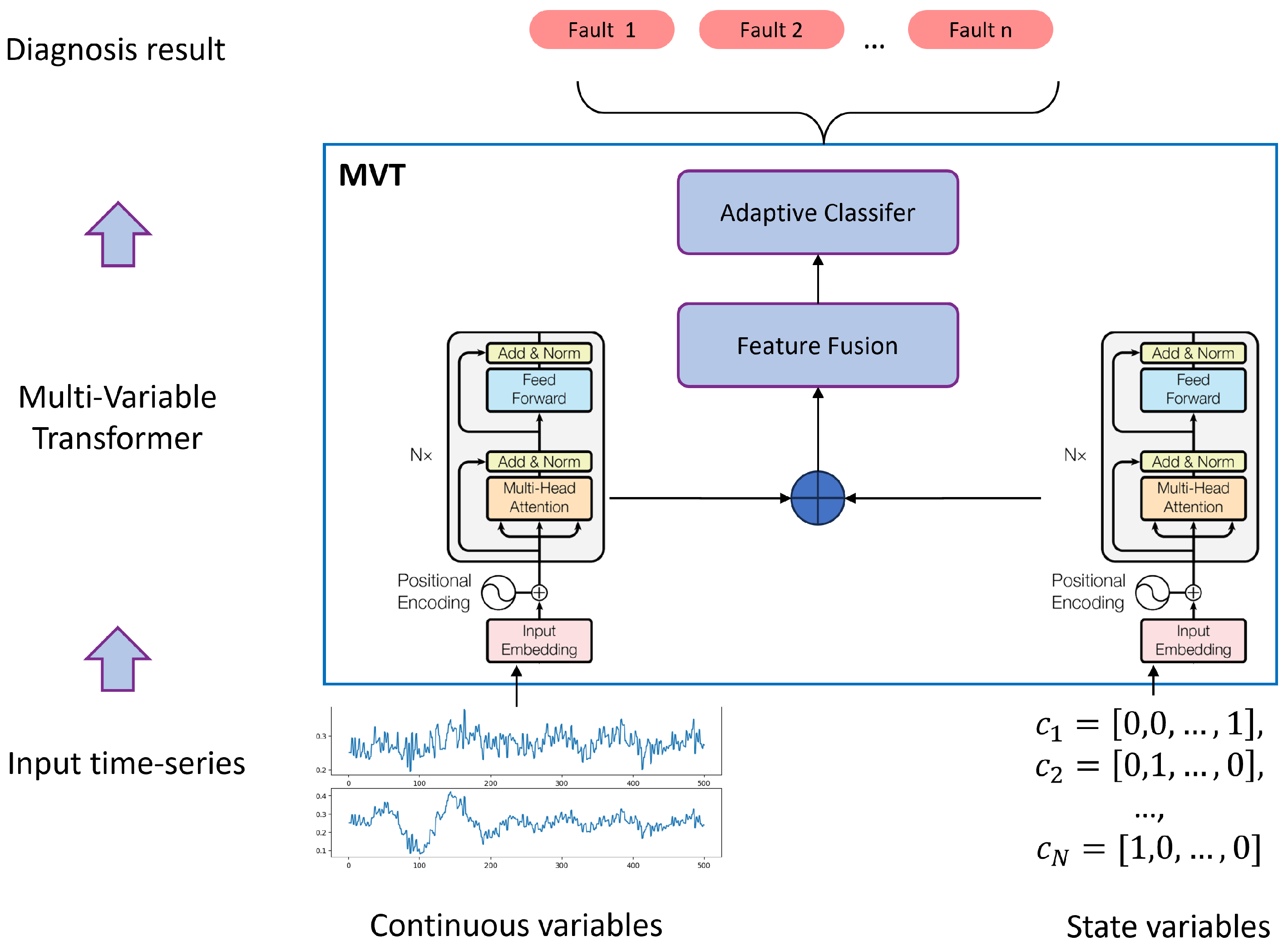
Table 5.
Task Settings for the TEP Dataset.
| Task Type | Dataset | Number of Fault Types | Support Samples | Query Samples | Sample Length |
|---|---|---|---|---|---|
| Task 1 | Meta-Training Set | 5 | 1 | 5 | 50 |
| Meta-Testing Set | 5 | 1 | 30 | 50 | |
| Task 2 | Meta-Training Set | 5 | 3 | 10 | 30 |
| Meta-Testing Set | 5 | 3 | 30 | 30 |
Table 6.
Satellite Data: Fault Types in Meta-Training and Meta-Testing Sets.
| Dataset | Selected Fault Types |
|---|---|
| Meta-Training Set | 0, 1, 5, 8, 9, 11, 12, 14, 16, 17, 18, 19, 20, 22 |
| Meta-Testing Set | 2, 3, 4, 6, 7, 10, 13, 15, 21, 23 |
Table 7.
Task Settings for the Satellite Telemetry Dataset.
| Task Setting | Dataset | Number of Fault Types | Support Samples | Query Samples | Sample Length |
|---|---|---|---|---|---|
| Task Setting 1 | Meta-Training Set | 5 | 5 | 10 | 30 |
| Meta-Testing Set | 5 | 5 | 30 | 30 | |
| Task Setting 2 | Meta-Training Set | 5 | 5 | 10 | 30 |
| Meta-Testing Set | 7 | 5 | 30 | 30 | |
| Task Setting 3 | Meta-Training Set | 5 | 3 | 10 | 50 |
| Meta-Testing Set | 5 | 3 | 30 | 50 |
Table 8.
Optimized Hyperparameters for Dataset 1.
| Model | Hidden Size | Feature Size | Attention Heads | Encoder Layers | Kernel Size |
|---|---|---|---|---|---|
| MVMT | 128 | 256 | 3 | 2 | – |
| LSTM | 32 | 224 | – | – | – |
| 1DCNN | 96 | 256 | – | – | 5 |
| ViT | 96 | 96 | 4 | 2 | – |
Table 9.
Optimized Hyperparameters for Dataset 2.
| Model | Hidden Size | Feature Size | Attention Heads | Encoder Layers | Kernel Size |
|---|---|---|---|---|---|
| MVMT | 256 | 256 | 8 | 4 | – |
| LSTM | 128 | 196 | – | – | – |
| 1DCNN | 128 | 256 | – | – | 7 |
| ViT | 96 | 96 | 4 | 2 | – |
Table 10.
Experimental Results on Dataset 1: Baseline Models.
| Task Setting | Setting 1 | Setting 2 |
|---|---|---|
| Method | Accuracy | Accuracy |
| 1DCNN | 33.67% | 38.00% |
| LSTM | 30.14% | 39.67% |
| ViT | 43.55% | 44.53% |
| MVT(proposed) | 44.15% | 43.76% |
Table 11.
Experimental Results on Dataset 1: Models with MAML Strategy.
| Task Setting | Setting 1 | Setting 2 | ||
|---|---|---|---|---|
| Method | Accuracy | Training Time (s) | Accuracy | Training Time (s) |
| 1DCNN+MAML | 52.73% | 706 | 60.94% | 903 |
| LSTM+MAML | 50.05% | 7749 | 61.33% | 7670 |
| ViT+MAML | 53.47% | 2826 | 63.80% | 3172 |
| MVMT(proposed) | 56.70% | 2867 | 68.00% | 3165 |
Table 12.
Experimental Results on Dataset 2.
| Task Setting | Setting 1 | Setting 2 | Setting 3 | |||
|---|---|---|---|---|---|---|
| Method | Accuracy | Training Time | Accuracy | Training Time | Accuracy | Training Time |
| 1DCNN | 16.30% | NaN | 14.50% | NaN | 19.52% | NaN |
| LSTM | 31.40% | NaN | 33.74% | NaN | 32.86% | NaN |
| ViT | 36.73% | NaN | 26.67% | NaN | 22.86% | NaN |
| MVT (proposed) | 31.67% | NaN | 41.33% | NaN | 33.64% | NaN |
| 1DCNN+MAML | 64.45% | 1353 | 43.63% | 1464 | 65.53% | 1814 |
| LSTM+MAML | 67.87% | 5258 | 60.00% | 5216 | 70.10% | 8750 |
| ViT+MAML | 78.40% | 2955 | 64.45% | 2778 | 80.20% | 3322 |
| MVMT (proposed) | 83.20% | 2652 | 72.10% | 2787 | 80.86% | 3001 |
| 1DCNN+meta-SGD | 68.9% | 1282 | 47.92% | 1550 | 69.87% | 1923 |
| LSTM+meta-SGD | 73.34% | 5250 | 60.00% | 5640 | 79.05% | 8917 |
| ViT+meta-SGD | 72.66% | 2821 | 67.14% | 2775 | 73.30% | 3174 |
| MVMT+meta-SGD (proposed) | 81.15% | 2542 | 73.00% | 2918 | 79.25% | 3111 |
Disclaimer/Publisher’s Note: The statements, opinions and data contained in all publications are solely those of the individual author(s) and contributor(s) and not of MDPI and/or the editor(s). MDPI and/or the editor(s) disclaim responsibility for any injury to people or property resulting from any ideas, methods, instructions or products referred to in the content. |
© 2025 by the authors. Licensee MDPI, Basel, Switzerland. This article is an open access article distributed under the terms and conditions of the Creative Commons Attribution (CC BY) license (http://creativecommons.org/licenses/by/4.0/).
Copyright: This open access article is published under a Creative Commons CC BY 4.0 license, which permit the free download, distribution, and reuse, provided that the author and preprint are cited in any reuse.


