Submitted:
03 April 2025
Posted:
04 April 2025
You are already at the latest version
Abstract
Proximal plant-based monitoring provides high-resolution data about trees, leading to more precise orchard management and in-depth knowledge about the tree physiology. The present work focuses on continuous real-time monitoring of olive cv. 'Ascolana Tenera' on an hourly time span during the third stage of fruit growth (mesocarp cell expansion) under mild water stress conditions (ψStem above -2 MPa). This is achieved by mounting dendrometers on the root, trunk, branch, and fruit to assess and model the behavior of each organ. The diameter variation of each organ at various time intervals (daily, two-weeks, and entire experiment), as well as their hysteretic patterns relative to each other and vapor pressure deficit, has been demonstrated. The results show different correlations between various organs, ranging from very weak to strongly positive. However, the trend of fruit versus root consistently shows a strong positive relationship throughout the entire experiment (R² = 0.83) and good across various two-week intervals (R² ranging from 0.54 to 0.93). Additionally, different time lags in dehydration and rehydration between organs were observed, suggesting that the branch is the most reactive organ, regulating dehydration and rehydration in the tree. Regarding the hysteretic pattern, different rotational patterns and characteristics (shape) were observed among the organs and in relation to vapor pressure deficit. This research provides valuable insight into the flow dynamics within a tree, models plant water relations and time lags in terms of water storage and transport and could be implemented for precise olive tree water status detection.
Keywords:
Olea europaea L.
; hysteresis
; continuous plant-based monitoring
; time lag
; diameter fluctuation
; dendrometer
; water flow dynamics
1. Introduction
Precise farming management involves high-resolution data collection from sources such as micro-climates, soil, plants, and fruits, followed by the implementation of appropriate agronomical practices [1,2]. In the olive, continuous monitoring aims at applying real-time optimization to orchard performance [3,4,5] and it can be obtained using proximal plant-based sensors mounted in contact with the surface of the organs of the plant such as the root, trunk, stem, leaves, and fruit [6,7].
This kind of sensing has been investigated in several studies on olives. For instance, Cuevas et al. [8] measured the trunk diameter variation to obtain an index for water stress. Brunetti et al. [9] used a custom leaf sensor to continuously monitor leaf water status as an applicable tool for precision irrigation. Khosravi et al. [10] monitored fruit diameter and simulated a model for olive maturation detection in the cultivar ‘Frantoio’. However, there are some challenges regarding the application of continuous monitoring using proximal plant-based sensors in olive orchard, such as the difficulty of replicating on many trees [11], and wide genetic diversity of olive, which leads to various physiological and morphological mechanisms, requiring the development of cultivar-specific thresholds [12], or developing not cultivar specific methods.
To deal with these challenges various solutions have been provided. Several research suggested the application of innovative methods for evaluation of sensor output data such as hysteresis phenomenon [13,14,15]. Hysteresis is defined as a non-linear loop-like behavior that does not show affine similarity with respect to time [14,16]. In olive, Khosravi et al. [5] developed a method using detection of different hysteresis curves for fruit diameter versus Vapor Pressure Deficit (VPD) and suggested a non-cultivar-specific model for setting quantitative index of water status detection. However, this method has been tested just on the Proximal fruit-based sensing and should be examined for other tree organs.
Another suggested solution was to combine non-continuously measured parameters with continuously measured data. Hernandez-Santana et al. [17] measured stomatal conductance in a non-continuous manner and correlated it with continuously measured sap flow. This study suggested the possibility of estimating stomatal conductance in olive trees automatically and continuously under field conditions by using sap flux data.
Some other advanced research combined different continuous plant-based measurements. Rodriguez-Dominguez et al. [18] used stem sap flow and leaf turgor pressure to model the response of trees regarding different levels of water stress and prioritized implementation of different sensors according to the different levels of stress. Marino et al. [4] combined three different sensors, including sap flow, leaf turgor pressure, and fruit gauge, to identify the most efficient one for detecting mild water stress in two Sicilian olive cultivars. The results suggested that a combination of sensors could detect water stress in olives earlier than a single sensor. Additionally, different responses were reported between these two olive cultivars. Therefore, more studies combining various sensors are needed to reveal different response of various organs and to establish more robust models in different climates and olive cultivars.
This research examined four different organs of the olive tree, including root, trunk, branch and fruit by mounting proximal plant-based sensors (dendrometer) to evaluate the evolution of each organ on the same tree during the third stage of olive fruit growth (mesocarp cell expansion). The specific objective was to continuously describe the behavior of the ‘Ascolana Tenera’ olive cultivar under mild water stress conditions. To our knowledge, no other studies have yet continuously monitored olive trees through root, trunk, branch and fruit diameters.
2. Materials and Methods
2.1. Site Description and Phenology
The experiment was conducted in 2023 in 14-years old olive trees (Olea europaea L., cv. ‘Ascolana Tenera’) at the commercial olive orchard of Olive Gregori, in Montalto delle Marche, Ascoli Piceno, Italy (latitude 42° 580 5700 N; longitude 13° 380 2100 E; altitude 310 m asl). The olive trees were planted with a northwest to southeast orientation, according to a 7.0 × 7.0 m array (204 trees per hectare) and trained as free open vase. The soil had a clay texture and the agricultural operations, pest control and fertilization practices were conducted in accordance with organic farming practices. The full bloom occurred on the 31st of May (DOY 151) and the pit hardening on the 29th of July (DOY 210). Olive trees were rainfed during 2023.
2.2. Plant Measurements
The diameter of root, trunk, branch, and fruit were monitored by automatic dendrometers from August 14th (DOY 226) to October 8th (DOY 281), 2023. Sensor’s installation consisted in two different sensors set. The first set of sensors (Ecomatik GmbH, Munich, Germany) was installed on 3 representative trees and consisted in one root dendrometer (model DD-RO), one trunk dendrometer (model DD-L1), two branch dendrometers (model DD-S2) and two fruit extensimeters (synonyms of fruit gauge/dendrometer, model DF6). This resulted in a total of 3 root dendrometers, 3 trunk dendrometers, 6 branch dendrometers, and 6 fruit extensimeters. The second set of sensors, installed in 3 representative trees consisted in a branch dendrometer and a fruit extensimeter of the same model as before, making a total of 3 branch dendrometers and 3 extensimeters. Totally we examined the diameter of 3 roots, 3 trunks, 9 branches, and 9 fruits. All sensors were connected to low-power Long Range Wide Area Network, (LoRaWAN) nodes (Ecomatik GmbH, Munich, Germany). The LoRa nodes were integrated via a LoRaWAN gateway, which establishes the connection to the Internet and the LoRa server for storing the measurement data.
Regarding the root dendrometer, the north-west side of the trunk at about 40 cm from the base was excavated to a depth of approximately 30 to 45 cm to locate a lateral root with a diameter of around 1 cm, upon which the dendrometer was mounted. Trunk dendrometers were installed on the northern side of the trunk at a height of about 40 cm from the ground, in areas free of scars and other irregularities. Fruit extensimeters were mounted on the same side of the trunk as the trunk dendrometers, at a height of about 1.2 meters and positioned at the midpoint of the canopy. Branch dendrometers were mounted on the same branch as the extensimeters.
The collected data underwent standardization using z-scores method [19] with the following equation:
where z is the standardized value, x is the value of the existing data, and mean is the average of all data and SD is the standard deviation. The standardized value could range from negative to positive value, according to the distance from the mean of the data.
z = (x−mean)/SD
On all the trees with the installed sensors, the stem water potential (ᴪStem) was measured at midday every 3 to 4 weeks (Table 1) using a pressure chamber (model 1000, PMS Instrument Co., Albany, OR, USA) on apical shoots (with 3-5 pairs of leaves) covered with aluminum foil approximately 1 hour before the reading [20]. These measurements were conducted during midday solar time. Table 1 shows that even though the trees were not irrigated, they maintained a mild water stress.
2.3. Meteorological Data
The climate of the study area is Mediterranean, and according to the Köppen–Geiger climate classification, Montalto delle Marche falls under the Cfb category, which is characterized by warm temperatures and high humidity, particularly during the summer months [21]. The meteorological data were sourced from the nearest Regional meteorological station (www.protezionecivile.marche.it), located approximately 6 km away from the orchard. Vapor Pressure Deficit (VPD) was computed using the formula recommended by Monteith and Unsworth [22]:
where RH is the relative humidity, SVP is the saturated vapor pressure and T is the temperature (°C).
VPD = (1 − (RH/100)) × SVP and SVP (Pascals) = 610.7 × 10^(7.5T/(237.3+T))
The VPD and rainfall data captured during the experiment (DOY 226 to DOY 281) are reported in Figure 1. The highest hourly VPD measured was 4.46 kPa on August 25th (DOY 237). The lowest value of VPD was 0.00 kPa on the 30th and 31st of August, as well as on the 14th, 15th, 16th, 17th, 18th, 23rd, 24th, 25th of September, and on the 5th of October (DOY 242, 243, 257, 258, 259, 260, 261, 266, 267, 268, and 278, respectively) due to an increase in relative humidity to 100%. The highest daily average of VPD was 2.71 kPa on August the 26th (DOY 238), whereas the lowest was 0.14 kPa on September the 15th (DOY 258). The daily mean VPD during the experiment was 1.23 ± 0.58 kPa.
Throughout the experimental period, the total cumulated rainfall was 42.4 mm, with peak hourly and daily values reaching 19.6 mm hour−1 and 20.6 mm day−1, respectively, recorded on September the 23rd (DOY 266).
2.4. Hysteresis Pattern
Considering hysteretic behavior as an indirect response of vegetation to diurnal changes in the external environment [23], the daily hysteretic pattern of different organs versus VPD has been monitored. VPD has been selected not only as one of the most significant variables but also as a driver for transpiration in plants due to its crucial role in plant growth and productivity [24]. To describe the hysteresis rotational pattern, the terms clockwise and anticlockwise were used. Additionally, the hysteresis form was characterized as either partial or complete. A partial hysteresis curve appeared only during part of day and did not represent the entire day. In contrast, a complete hysteresis loop represents the entire day (see [5,15]).
2.5. Data Analysis and Visualization
Descriptive statistics were conducted on the output of different sensors, obtaining the mean, maximum, minimum and standard deviation. A regression analysis was performed to evaluate the linear relationship between the organs over the entire experiment period and across four different time intervals. The coefficient of determination (R2) was calculated. Data analysis and graph visualization were performed using SigmaPlot 14.5 (Systat Software, Inc., San Jose, CA, USA).
3. Results
3.1. Fruit, Branch, Trunk and Root Sensing
Standardized diameter measurements throughout the experiment period are presented for root (Figure 2D), trunk (Figure 2C), branch (Figure 2B), and fruit (Figure 2A). Considering the initial and the ending point of experiment, Table 2 displays the growth in standardized diameter for all the considered organs. Interestingly the growth rate was not the same among the different organs. The root showed the highest increase in the standardized diameter (3.37 units), followed by the fruit (3.28), trunk (2.95) and branch (1.64).
Furthermore, there was notable daily diameter fluctuation in all the organs with different rates. The highest daily diameter fluctuation was found for the branch, followed by the trunk, and the lowest was registered for the fruit, followed by the root (Figure S1).
Regarding the correlation among different organs, a strong relationship was observed between the trunk and the fruit (R² = 0.93) and the trunk and root (R² = 0.90), followed by a moderately strong correlation between the fruit and the root (R² = 0.83). Conversely, moderate-to-weak correlations were found between the branch and the root (R² = 0.57) and the branch and the fruit (R² = 0.45) (Figure 3).
These various associations suggest different degrees of influence or interaction between the studied components. However, considering the physiological changes during the different stages of the plant growth, capturing the mentioned associations throughout shorter intervals is beneficial. Therefore, the experimental period is divided into four time-intervals, each lasting 14 days (Figure S2).
The trend for the root vs. the fruit exhibited a relatively consistent, strong, positive relationship across the four intervals, with R-squared values ranging from 0.54 to 0.93 (Table 3). On the contrary, there was minimal or very weak correlation between the other organs (ranging from R² = 0 to 0.49), with an exception in the third interval (from 254 to 267 DOYs with intense rains), where a strong correlation between root and trunk (R² = 0.95), trunk and fruit (R² = 0.83), and moderately strong correlation between root and branch (R² = 0.63) and trunk and branch (R² = 0.65) were observed.
3.2. Daily Trend of Fruit, Branch, Trunk and Root and Hysteresis Curves Versus VPD
Regarding the daily pattern of the sensors, the root in 60.7% of cases (34 out of 56), the trunk in 91.1% of cases (51 out of 56), and the branch in 98.2% of cases (55 out of 56) were characterized by shrinkage from mid-morning to early afternoon, followed by an expansion from late afternoon to early morning (Figure 4). However, the duration, initial point, finishing point, and slope of daily shrinkage and expansion were dissimilar among different organs. The shrinkage for the root and trunk started around 6:00 to 8:00, while for the branch started around 4:00 to 6:00. The expansion for the root and trunk began around 15:00 to 17:00, whereas for the branch started around 13:00 to 15:00 (Table S1). For the fruit, this daily pattern was observed only in 41.1% of cases (23 out of 56) (Figure 4) with starting shrinkage around 8:00 to 9:00 and expansion around 17:00 to 18:00 (Table S1). In the remaining cases (33 out of 56), the daily trend for the fruit diameter was observed as an increase, with variations in duration and slope across different hours and days (Figure S3).
In most of the cases, the circadian variation of the diameter versus VPD formed a hysteresis curve, although with varying magnitude, frequency, and rotational pattern (Figure 5).
In details, the hysteresis loops of diameter versus VPD were observed in 66.1% of cases (37 out of 56) for the fruit, 87.5% of cases (49 out of 56) for the branch, 94.3% of cases (50 out of 53) for the trunk, and 64.3% of cases (36 out of 56) for the root. The rotational pattern of the hysteretic pattern for fruit, trunk and root was clockwise, whereas for the branch it was anticlockwise (Table 4).
Moreover, hysteretic patterns among each organ were observable, like before, with varying magnitude, frequency and rotational patterns (Figure 6). The most frequent daily hysteresis was formed in the relation between the branch and trunk in 100% of the cases (56 out of 56), while the least frequent one was observed between the fruit and root in 33.9% of the cases (19 out of 56) (Table 4).
4. Discussion
The daily trends of the fruit, branch, and trunk were consistent with the expectations: shrinkage from mid-morning to early afternoon, followed by an expansion from late afternoon to early morning. The highest variation rate was in the branch and could be due to the synergistic effect of water absorption by both fruits and leaves, which created the largest daily fluctuation compared to fruit and trunk. Regarding the daily dynamics of the olive root, there are no previous research studies to compare with our results; however, it could be described similarly to the other considered organs (trunk, branch, and fruit) but with higher daily variability in recorded data compared to the other organs. This variability could be influenced by other factors such as soil/root hydraulic [25], dynamic of wetting and drying [26], root temperature and biomass [27]. Another type of continuous olive root monitoring, not using a dendrometer, was conducted by Villalobos et al. [28], where they measured diurnal variation of root conductance by combining microtensiometers and sap flow sensors. This approach was based on simultaneous determinations of sap flow and xylem water potential, which allowed them to estimate the temporal variations of root hydraulic conductance in olive trees. It was observed that root hydraulic conductance was proportional to transpiration, and the daily variation showed an inverted pattern than the diameter measured in our trial, that is an increase during the day and decrease in the night. Although the actual regulator of these changes was not identified.
It can be hypothesized that the continuous flow of water from root to fruit, affected by VPD, creates similar daily fluctuations in the root and the other organs. Additionally, since the trees used for our experiment did not experience severe water stress (Table 1), we observed a quick response of the root system to available water [29], resulting in a visible uniformity in daily diameter fluctuations (shrinkage and expansion) between the root and the other organs.
It is interesting how the shrinkage occurs with a different timeline among the considered organs: first occurring in the branch, followed by the trunk and root (simultaneously), and finally in the fruit (Table S1). This could be due to the water transpiration of the leaves, which affects the branch first and then moves toward the trunk and root. The withdrawal of water from internal storage compartments can contribute to 10–50% of a tree's daily water usage, depending on factors such as species, ecosystem type, and tree size [30,31]. Water storage as a homeostatic mechanism is particularly crucial in olive trees. During peak transpiration, they rely on stored water, which is later replenished, allowing roots to absorb water at moderate rates over an extended period [31]. In the expansion phase, the branch is again the first organ to react (expand), followed by the trunk and root (simultaneously), and finally the fruit (Table S1). These aspects are more evident in Figure 6, where the best hysteretic curve (loop-like behavior) is observed in the branch versus fruit, showing the highest time lag between the start of shrinkage in the branch (4:00 to 6:00) and fruit (8:00 to 9:00) and the start of expansion in the branch (13:00 to 15:00) and fruit (17:00 to 18:00). Consequently, a more obvious hysteretic pattern is observable, while the mentioned time lags in the trunk versus root are the lowest; therefore, the hysteretic magnitude in root versus trunk is not very clear. The time lag in dehydration and rehydration in different organs could be used as a signal for detecting different levels of water stress or as a time sensitive early warning for irrigation management. Interestingly, the time lag in rehydration was described in other fruits, such as nectarines, by Scalisi et al, [32], where they continuously monitored fruit and leaf hydration and explain that it could represent an early warning for water stress not influenced by the fruit development stage.
We could assume that through all studied organs in this research, considering the initial time of shrinkage and expansion (Table S2), higher daily fluctuation (Figure S2) as well different rotational pattern of hysteresis versus VPD (anticlockwise), branch is the most reactive organ which regulate dehydration and rehydration in tree.
The hysteretic pattern is an indirect response of vegetation to diurnal changes in the external environment [23], with VPD being the major factor affecting the diurnal hysteresis loop [13,15]. In our study, among organs, the trunk showed the highest frequency of hysteresis curve appearance versus VPD, followed by the branch. About the relation of organ between each other, the relationship between trunk and branch showed the highest frequency of hysteresis curve appearance, followed by the branch versus root, and the trunk versus root. This suggests that the trunk and branch are suitable indicators for hysteretic pattern recognition, serving as useful tools for precision tree management. Although, in our research the frequency of daily hysteretic pattern of fruit versus VPD was lower compared to the other organs, another study by Khosravi et al. [5] examined four different olive cultivars under deficit irrigation regime and demonstrate that magnitude of daily hysteresis curve of fruit versus VPD could be used as a non-cultivar specific index for monitoring water status. Therefore, it can be expected that this non cultivar specific index could be observed among organs with the highest frequency of hysteresis curve appearance versus VPD, such as the trunk. The lower frequency of the daily hysteretic pattern of fruit versus VPD could be a result of rain [10]), as rain can alter the daily dynamics of olive fruit growth by affecting the relative growth rate of the fruit [33]. The hysteretic pattern of the olive trunk was also reported by Fernández et al. [34], who showed a hysteresis curve with varying magnitudes in the relationship between diurnal courses of trunk diameter variation and sap flux. They observed the same trend in trunk diameter variation as we did. Additionally, they mentioned that when using trunk-based indices, factors such as plant age, size, and crop load should be considered. Another study by Moriana et al. [35] reported similar results regarding trunk variation. Furthermore, they noted that the relationship between trunk-derived indices of maximum daily shrinkage (MDS) and midday stem water potential values of -1.5 MPa or greater (under light water stress conditions, as in our experiment) is linear, with increasing MDS values corresponding to a decrease in stem size. The authors proposed that the reduction in MDS might be caused by decreased transpiration due to the progressive closure of stomata under severe water stress. They concluded that, although there isn't a direct relationship between MDS and stem diameter in olive trees, the observed response patterns could be explained by the effects of transpiration and soil water deficits on both variables.
The results of our study showed a good correlation between olive root and fruit in both the long term (entire experiment) and the short term (14-day intervals) (Table 3 and Figure 3). This suggests that the root and fruit are well-aligned. It suggests that to monitor the flow dynamics within a tree and model plant water relations and time lags in terms of water storage and transport capacities, fruit and root data could be effectively coordinated.
However, with the increasing available water caused by rain in the third time interval (DOY 254 to 267), the correlation between root and trunk increased notably. This could be the result of positive root pressure due to the rising soil humidity level and, at the same time, a decrease in the average VPD during this time interval (Table S2). This change in the correlations between parameters throughout the season could be caused by variations in the radial resistance between xylem and bark on a diurnal and seasonal basis, which affects the water flux between these two tissues [36]. Therefore, trees need to optimize water flow through their tissue compartments and ensure a certain level of coordination between capacitance, vertical water flux in the xylem, transpiration, and radial water movement in the phloem [31].
5. Conclusions
Our study presents insights into the organ correlations within olive trees, particularly in relation to water storage and transport under mild water stress conditions. The daily shrinkage and expansion patterns of the fruit, branch, trunk, and root followed expected trends, with the branch playing a role to control the process of dehydration and rehydration, likely due to its function in the different leaf and fruit water use. The observed hysteretic patterns, particularly the strong relationship between the trunk and branch versus VPD, suggest that these organs are useful indicators for precise water status detection and irrigation management. Additionally, the significant correlations between the root and fruit indicate the potential for coordinated monitoring of plant water relations, while the influence of rain on the dynamics between the root and trunk highlights the complexity of environmental factors affecting tree water balance. The findings underscore the importance of considering time lags in organ dehydration and rehydration as priority means of physiological coordination and early signals of water stress, offering a practical tool for optimizing orchard management and irrigation practices. Further research can focus on the application of different levels of water stress and on considering different olive cultivars, as olive species (Olea europaea L) has a very wide genetic diversity.
Supplementary Materials
The following supporting information can be downloaded at the website of this paper posted on Preprints.org, Figure S1: The daily trends of diameter fluctuation throughout the experiment period.; Figure S2: Continuous measurements of diameter of olive fruit, branch, trunk and root in four time-intervals, each lasting 14 days: (A) from DOY 226 to DOY 239; (B) from DOY 240 to DOY 253; (C) from DOY 254 to DOY 267; (D) from DOY 268 to DOY 281. Data of fruit and branch represent the average of nine replicates, while data of trunk and root represent the average of three replicates. Missing data from 238 to 241 day of the year (DOY) for trunk diameter. For better illustration of daily fluctuation of each single organs, different range for y axis has been employed; Figure S3: Continuous measurements of diameter of olive fruit in two single day interval of the experiment with continuous growth trend. A: 22th of September (DOY 265); B: 30th of September (DOY 273). For better illustration of daily fluctuation, different range for y axis has been employed; Table S1: Starting time of shrinkage and expansion for different organs during entire experiment period; Table S2: Weather parameters in four intervals.
Author Contributions
Conceptualization, D.N., A.K., E.M.L. and V.G.; methodology, A.K. and F.B.; software, A.M. and A.K; investigation, D.N.; data curation, A.K. and A.M.; writing—original draft preparation, A.K.; writing—review and editing, D.N., A.K., V.G, E.M.L. and F.B.; visualization, A.K.; supervision, D.N.; project administration, D.N.; funding acquisition, D.N. All authors have read and agreed to the published version of the manuscript.
Funding
This research was partially funded by: TeneRa project of the operational group RiTA (ID 59750), “Valorization of genetic resources and introduction of innovative techniques for Ascolana tenera production” founded by PSR Marche 2014-2020 (16.1) and European Union – Next Generation EU. Project Code: ECS00000041; Project CUP: C43C22000380007; Project Title: Innovation, digitalization and sustainability for the diffused economy in Central Italy – VITALITY.
Data Availability Statement
All data are available with an email request to the authors
Acknowledgments
Olive Gregori Farm, in Montalto delle Marche, Ascoli Piceno, Italy
Conflicts of Interest
The authors declare no conflict of interest.
References
- Shafi, U.; Mumtaz, R.; García-Nieto, J.; Hassan, S.A.; Zaidi, S.A.R.; Iqbal, N. Precision Agriculture Techniques and Practices: From Considerations to Applications. Sensors 2019, 19, 3796. [Google Scholar] [CrossRef]
- Zude-Sasse, M.; Fountas, S.; Gemtos, T.; Abu-Khalaf, N. Applications of precision agriculture in horticultural crops. Eur. J. Hortic. Sci. 2016, 81, 78–90. [Google Scholar] [CrossRef]
- Scalisi, A.; Marino, G.; Marra, F.P.; Caruso, T.; Bianco, R.L. A Cultivar-Sensitive Approach for the Continuous Monitoring of Olive (Olea europaea L.) Tree Water Status by Fruit and Leaf Sensing. Front. Plant Sci. 2020, 11, 340. [Google Scholar] [CrossRef]
- Marino, G.; Scalisi, A.; Guzmán-Delgado, P.; Caruso, T.; Marra, F.P.; Bianco, R.L. Detecting Mild Water Stress in Olive with Multiple Plant-Based Continuous Sensors. Plants 2021, 10, 131. [Google Scholar] [CrossRef]
- Khosravi, A.; Zucchini, M.; Mancini, A.; Neri, D. Continuous Third Phase Fruit Monitoring in Olive with Regulated Deficit Irrigation to Set a Quantitative Index of Water Stress. Horticulturae 2022, 8, 1221. [Google Scholar] [CrossRef]
- Morandi, B.; Manfrini, L.; Zibordi, M.; Noferini, M.; Fiori, G.; Grappadelli, L.C. A Low-cost Device for Accurate and Continuous Measurements of Fruit Diameter. HortScience 2007, 42, 1380–1382. [Google Scholar] [CrossRef]
- Sishodia, R.P.; Ray, R.L.; Singh, S.K. Applications of Remote Sensing in Precision Agriculture: A Review. Remote. Sens. 2020, 12, 3136. [Google Scholar] [CrossRef]
- Cuevas, M.; Torres-Ruiz, J.; Álvarez, R.; Jiménez, M.D.; Cuerva, J.; Fernández, J. Assessment of trunk diameter variation derived indices as water stress indicators in mature olive trees. Agric. Water Manag. 2010, 97, 1293–1302. [Google Scholar] [CrossRef]
- Brunetti, C., Alderotti, F., Pasquini, D., Stella, C., Gori, A., Ferrini, F., ... & Centritto, M. (2022). On-line monitoring of plant water status: Validation of a novel sensor based on photon attenuation of radiation through the leaf. Science of The Total Environment, 817, 152881.
- Khosravi, A.; Zucchini, M.; Giorgi, V.; Mancini, A.; Neri, D. Continuous Monitoring of Olive Fruit Growth by Automatic Extensimeter in Response to Vapor Pressure Deficit from Pit Hardening to Harvest. Horticulturae 2021, 7, 349. [Google Scholar] [CrossRef]
- Fernández, J. Plant-based sensing to monitor water stress: Applicability to commercial orchards. Agric. Water Manag. 2014, 142, 99–109. [Google Scholar] [CrossRef]
- Bianco, R.L.; Scalisi, A. Water relations and carbohydrate partitioning of four greenhouse-grown olive genotypes under long-term drought. Trees 2016, 31, 717–727. [Google Scholar] [CrossRef]
- Zeppel, M.J.B.; Murray, B.R.; Barton, C.; Eamus, D. Seasonal responses of xylem sap velocity to VPD and solar radiation during drought in a stand of native trees in temperate Australia. Funct. Plant Biol. 2004, 31, 461–470. [Google Scholar] [CrossRef]
- Zhang, Q.; Manzoni, S.; Katul, G.; Porporato, A.; Yang, D. The hysteretic evapotranspiration—Vapor pressure deficit relation. J. Geophys. Res. Biogeosciences 2014, 119, 125–140. [Google Scholar] [CrossRef]
- Zucchini, M.; Khosravi, A.; Giorgi, V.; Mancini, A.; Neri, D. Is There Daily Growth Hysteresis versus Vapor Pressure Deficit in Cherry Fruit? Horticulturae 2021, 7, 131. [Google Scholar] [CrossRef]
- Mayergoyz, I. D. (2003). Mathematical models of hysteresis and their applications. Academic press.
- Hernandez-Santana, V.; Fernández, J.; Rodriguez-Dominguez, C.; Romero, R.; Diaz-Espejo, A. The dynamics of radial sap flux density reflects changes in stomatal conductance in response to soil and air water deficit. Agric. For. Meteorol. 2016, 218-219, 92–101. [Google Scholar] [CrossRef]
- Rodriguez-Dominguez, C.; Ehrenberger, W.; Sann, C.; Rüger, S.; Sukhorukov, V.; Martín-Palomo, M.; Diaz-Espejo, A.; Cuevas, M.; Torres-Ruiz, J.; Perez-Martin, A.; et al. Concomitant measurements of stem sap flow and leaf turgor pressure in olive trees using the leaf patch clamp pressure probe. Agric. Water Manag. 2012, 114, 50–58. [Google Scholar] [CrossRef]
- Bird, J. (2014). Engineering mathematics. Routledge.
- Caruso, G.; Palai, G.; Tozzini, L.; Gucci, R. Using Visible and Thermal Images by an Unmanned Aerial Vehicle to Monitor the Plant Water Status, Canopy Growth and Yield of Olive Trees (cvs. Frantoio and Leccino) under Different Irrigation Regimes. Agronomy 2022, 12, 1904. [Google Scholar] [CrossRef]
- Peel, M.C.; Finlayson, B.L.; McMahon, T.A. Updated world map of the Köppen-Geiger climate classification. Hydrol. Earth Syst. Sci. 2007, 11, 1633–1644. [Google Scholar] [CrossRef]
- Monteith, J., & Unsworth, M. (2013). Principles of environmental physics: plants, animals, and the atmosphere. Academic press.
- Zhang, R.; Xu, X.; Liu, M.; Zhang, Y.; Xu, C.; Yi, R.; Luo, W.; Soulsby, C. Hysteresis in sap flow and its controlling mechanisms for a deciduous broad-leaved tree species in a humid karst region. Sci. China Earth Sci. 2019, 62, 1744–1755. [Google Scholar] [CrossRef]
- Amitrano, C.; Arena, C.; Rouphael, Y.; De Pascale, S.; De Micco, V. Vapour pressure deficit: The hidden driver behind plant morphofunctional traits in controlled environments. Ann. Appl. Biol. 2019, 175, 313–325. [Google Scholar] [CrossRef]
- O'Brien, J.J.; Oberbauer, S.F.; Clark, D.B. Whole tree xylem sap flow responses to multiple environmental variables in a wet tropical forest. Plant, Cell Environ. 2004, 27, 551–567. [Google Scholar] [CrossRef]
- Gucci, R.; Lodolini, E.M.; Rapoport, H.F. Water deficit-induced changes in mesocarp cellular processes and the relationship between mesocarp and endocarp during olive fruit development. Tree Physiol. 2009, 29, 1575–1585. [Google Scholar] [CrossRef]
- Miserere, A.; Searles, P.S.; Manchó, G.; Maseda, P.H.; Rousseaux, M.C. Sap Flow Responses to Warming and Fruit Load in Young Olive Trees. Front. Plant Sci. 2019, 10, 1199. [Google Scholar] [CrossRef]
- Villalobos, F.J.; Testi, L.; García-Tejera, O.; López-Bernal, Á.; Tejado, I.; Vinagre, B.M. Measuring the Diurnal Variation of Root Conductance in Olive Trees Using Microtensiometers and Sap Flow Sensors. Plant Soil 2024, 1–14. [Google Scholar] [CrossRef]
- Clothier, B.E.; Green, S.R.; Moreno, F.; Fernández, J.E. Transpiration and root water uptake by olive trees. Plant Soil 1996, 184, 85–96. [Google Scholar] [CrossRef]
- Scholz, F.G.; Phillips, N.G.; Bucci, S.J.; Meinzer, FG.C.; Goldstein, G. 2011. Hydraulic capacitance: biophysics and functional significance of internal water sources in relation to tree size. In Size- and Age-related Changes in Tree Structure and Function, Meinzer FC, Lachenbruch B, Dawson TE (eds). New York: Springer; 341–362.
- Cocozza, C.; Marino, G.; Giovannelli, A.; Cantini, C.; Centritto, M.; Tognetti, R. Simultaneous measurements of stem radius variation and sap flux density reveal synchronisation of water storage and transpiration dynamics in olive trees. Ecohydrology 2014, 8, 33–45. [Google Scholar] [CrossRef]
- Scalisi, A.; O’connell, M.G.; Stefanelli, D.; Bianco, R.L. Fruit and Leaf Sensing for Continuous Detection of Nectarine Water Status. Front. Plant Sci. 2019, 10, 805. [Google Scholar] [CrossRef]
- Khosravi, A.; Zucchini, M.; Mancini, A.; Lodolini, E.M.; Neri, D. Continuous Monitoring of olive fruit growth by Proximal Sensor: Case study of the Daily Rain Effect. 2023 IEEE International Workshop on Metrology for Agriculture and Forestry (MetroAgriFor). LOCATION OF CONFERENCE, ItalyDATE OF CONFERENCE; pp. 273–276.
- Fernández, J.E.; Moreno, F.; Martín-Palomo, M.J.; Cuevas, M.V.; Torres-Ruiz, J.M.; Moriana, A. Combining sap flow and trunk diameter measurements to assess water needs in mature olive orchards. Environ. Exp. Bot. 2011, 72, 330–338. [Google Scholar] [CrossRef]
- Moriana, A.; Fereres, E.; Orgaz, F.; Castro, J.; Humanes; Pastor, M. THE RELATIONS BETWEEN TRUNK DIAMETER FLUCTUATIONS AND TREE WATER STATUS IN OLIVE TREES (Olea europea L.). Acta Hortic. 2000, 293–297, https://doi.org/10.17660/actahortic.2000.537.33. [CrossRef]
- Meinzer, F.C.; Johnson, D.M.; Lachenbruch, B.; McCulloh, K.A.; Woodruff, D.R. Xylem hydraulic safety margins in woody plants: coordination of stomatal control of xylem tension with hydraulic capacitance. Funct. Ecol. 2009, 23, 922–930. [Google Scholar] [CrossRef]
Figure 1.
The hourly and daily trends of vapor pressure deficit (VPD) and rainfall throughout the experiment period (from day 226 to day 282 of the year, DOY) were obtained from the nearest Regional meteorological station (protezionecivile.marche.it).
Figure 1.
The hourly and daily trends of vapor pressure deficit (VPD) and rainfall throughout the experiment period (from day 226 to day 282 of the year, DOY) were obtained from the nearest Regional meteorological station (protezionecivile.marche.it).

Figure 2.
Continuous measurements of diameter of olive fruit, branch, trunk and root during the experiment period (from DOY 226 to DOY 282): (A) fruit; (B) branch; (C) trunk; (D) root. A and B represent the average of nine replicates, while C and D represent the average of three replicates. Missing data from 238 to 241 day of the year (DOY) for trunk diameter. For the trunk diameter (C) some data are missing due to a malfunctioning of the IOP.
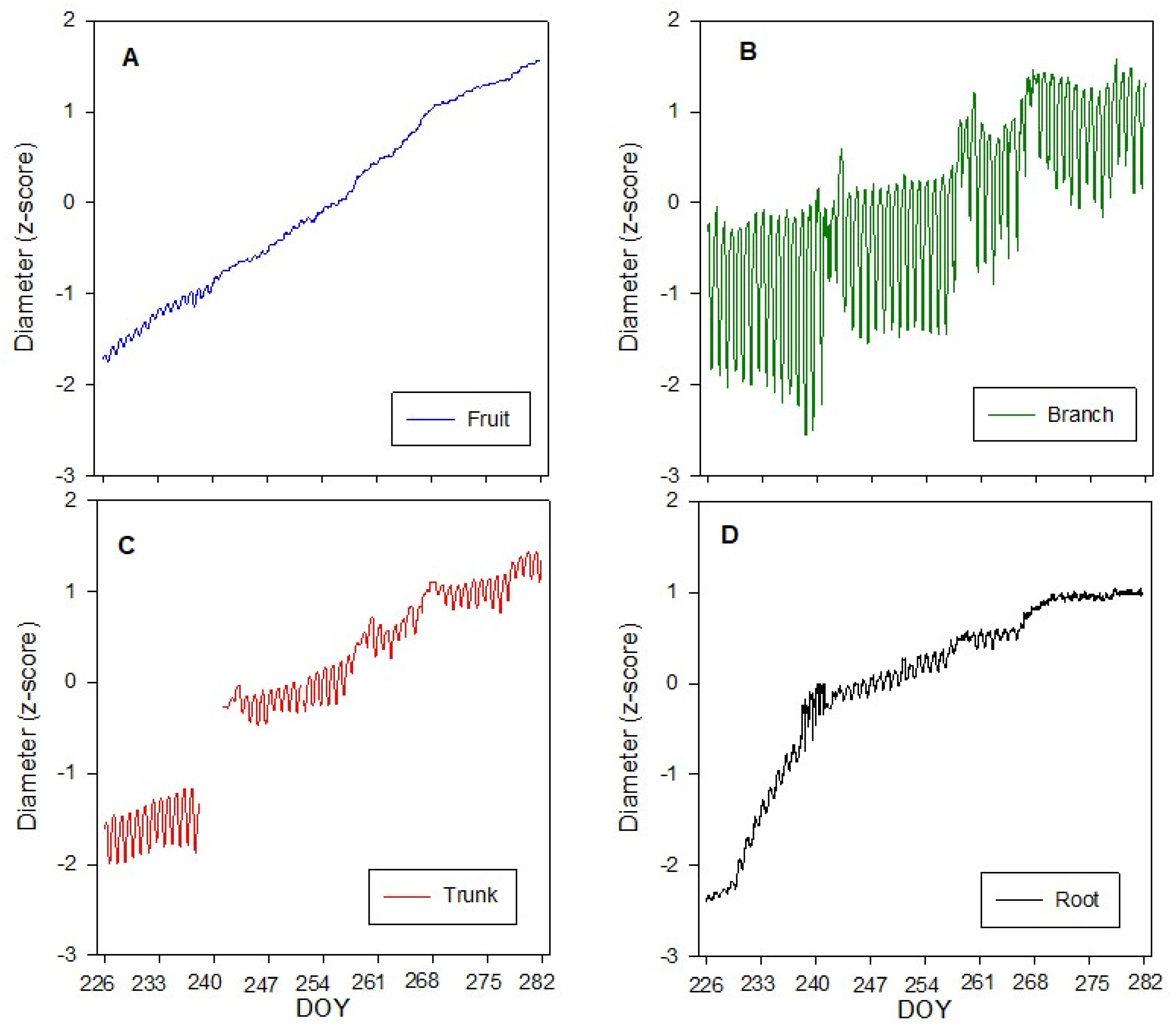
Figure 3.
Linear regression comparison of different tree organs during the experiment period (from DOY 226 to DOY 282). Blue lines represent confidence intervals, and red lines indicate predictions.
Figure 3.
Linear regression comparison of different tree organs during the experiment period (from DOY 226 to DOY 282). Blue lines represent confidence intervals, and red lines indicate predictions.
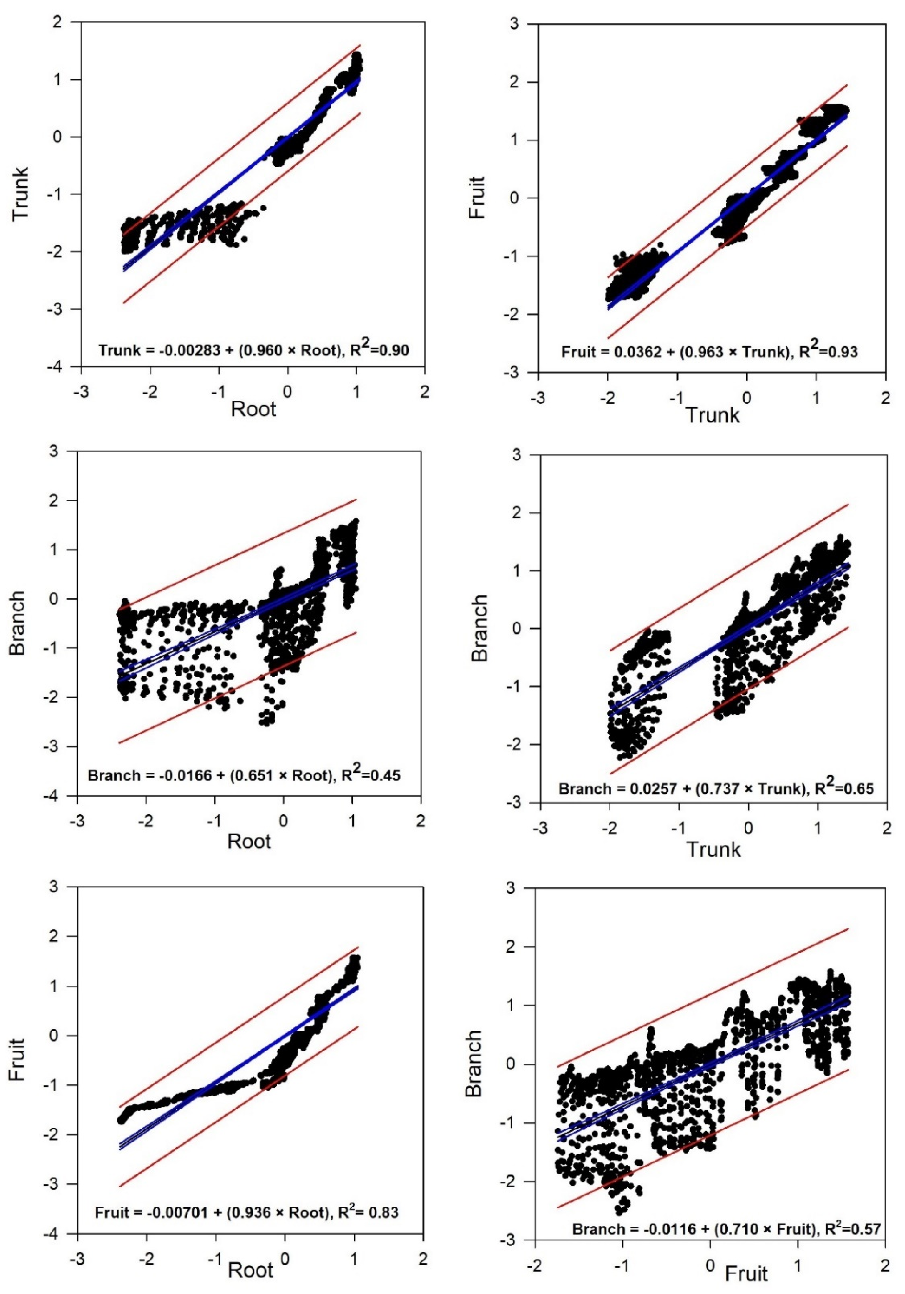
Figure 4.
Continuous measurements of diameter of the fruit, branch, trunk and root on a single day interval of the experiment (DOY 228). Fruit and branch represent the average of nine replicates, while root and trunk represent the average of three replicates. For better illustration of daily fluctuation of each single organ, a different range for y axis has been used. .
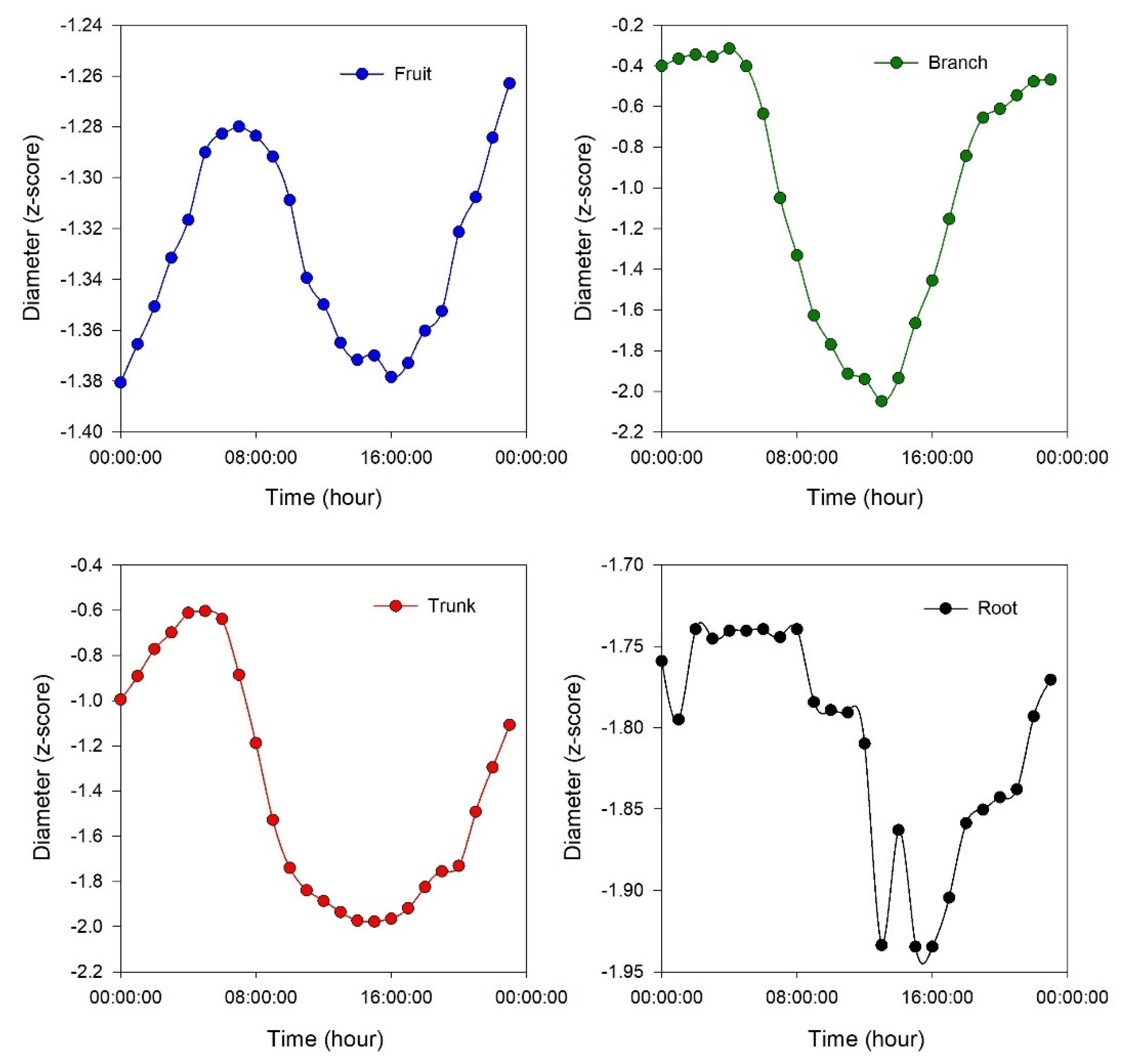
Figure 5.
Hysteresis curves of the diameter of the fruit, branch, trunk and root versus the Vapor Pressure Deficit (VPD) on a single day interval of the experiment (DOY 235). The yellow point shows the starting point of the curve, and the arrowed black lines show the rotational pattern. For better illustration of daily hysteresis curve of each single organ, a different range for y axis has been used.
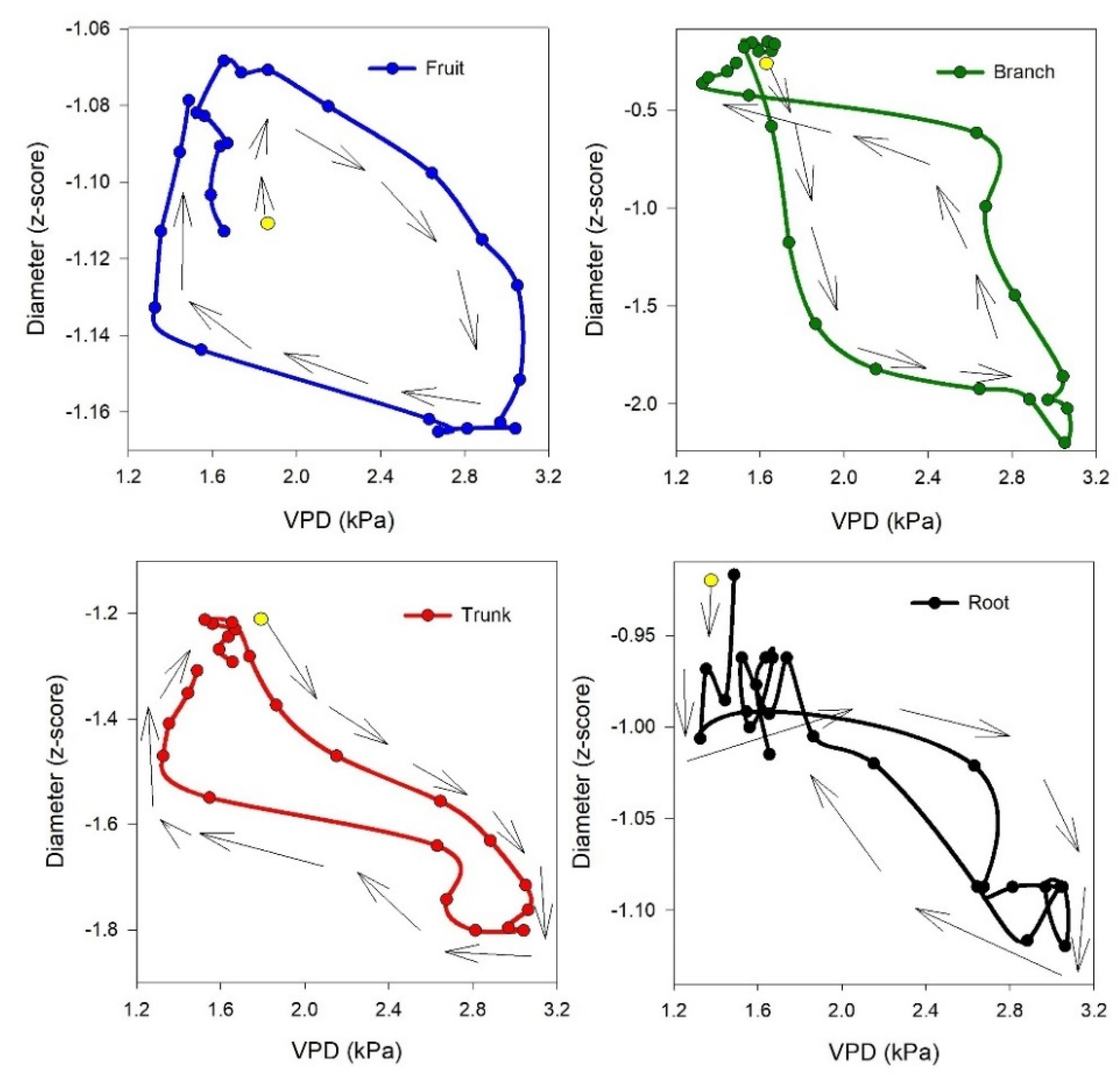
Figure 6.
The hysteresis curves of different plant organs in relation to each other on a single day interval of the experiment (DOY 235). The yellow point shows the starting point of the curves, and the arrowed black lines show the rotational pattern. For better illustration of daily hysteresis curves, a different range for y axis has been used.
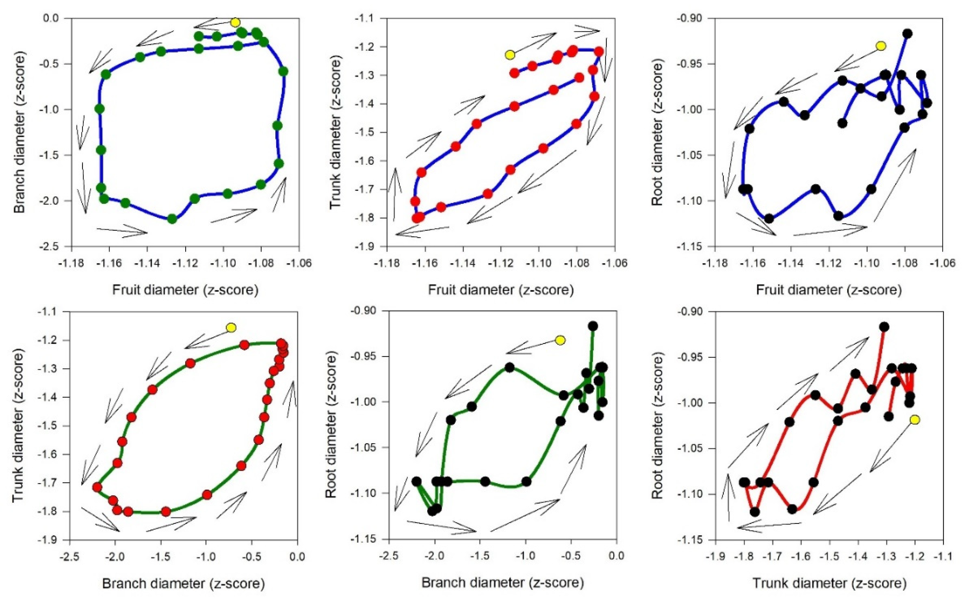

Table 1.
Stem water potential (ᴪStem) from DOY 194 to DOY 265. Each value represents the average of fifteen measurements.
Table 1.
Stem water potential (ᴪStem) from DOY 194 to DOY 265. Each value represents the average of fifteen measurements.
| DOY | ᴪStem (MPa) |
|---|---|
| 194 | -1.49 ± 0.18 |
| 213 | -1.89 ± 0.22 |
| 240 | -1.89 ± 0.20 |
| 265 | -1.36 ± 0.03 |
Table 2.
Statistical indices of different organs of the trees for the entire experimental period.
| Description | Number of records | Mean | Max | Min | Std. Dev | Initial point | Ending point |
|---|---|---|---|---|---|---|---|
| Fruit | 1344 | -0.009 | 1.57 | -1.74 | 0.99 | -1.71 | 1.57 |
| Branch | 1344 | -0.018 | 1.58 | -2.54 | 0.93 | -0.32 | 1.32 |
| Trunk | 1272 | 1.3 E-11 | 1.44 | -1.99 | 1.00 | -1.60 | 1.35 |
| Root | 1344 | -0.003 | 1.05 | -2.39 | 0.97 | -2.39 | 0.98 |
Table 3.
R-squared (R2) values of linear regression between the organs across four different time intervals of the experiment.
Table 3.
R-squared (R2) values of linear regression between the organs across four different time intervals of the experiment.
|
Description |
226 to 239 (DOY) |
240 to 253 (DOY) |
254 to 267 (DOY) |
268 to 281 (DOY) |
|---|---|---|---|---|
| Root vs Trunk | 0.22 | 0.49 | 0.95 | 0.29 |
| Root vs Branch | 0.00 | 0.06 | 0.63 | 0.00 |
| Root vs Fruit | 0.93 | 0.69 | 0.81 | 0.54 |
| Trunk vs Branch | 0.44 | 0.27 | 0.65 | 0.29 |
| Trunk vs Fruit | 0.29 | 0.20 | 0.83 | 0.42 |
| Branch vs Fruit | 0.00 | 0.00 | 0.34 | 0.00 |
Table 4.
Frequency of appearance of different hysteresis curves and rotational patterns, and frequency of days with no hysteresis pattern for different sensor outputs versus VPD and versus each other during the entire experiment period. There are 4 missing data points for fruit vs branch, fruit vs trunk, branch vs trunk, and trunk vs root, and 3 missing data points for trunk vs VPD.
| Description | Complete | Partial | Rotational pattern | No hysteresis |
|---|---|---|---|---|
| Fruit vs VPD | 5 | 32 | Clockwise | 19 |
| Branch vs VPD | 26 | 23 | Anticlockwise | 7 |
| Trunk vs VPD | 32 | 18 | Clockwise | 3 |
| Root vs VPD | 19 | 17 | Clockwise | 20 |
| Fruit vs Branch | 5 | 28 | Anticlockwise | 19 |
| Fruit vs Trunk | 2 | 29 | Clockwise | 21 |
| Fruit vs Root | 4 | 15 | Anticlockwise | 37 |
| Branch vs Trunk | 46 | 6 | Anticlockwise | 0 |
| Branch vs Root | 20 | 23 | Anticlockwise | 13 |
| Trunk vs Root | 28 | 11 | Clockwise | 13 |
Disclaimer/Publisher’s Note: The statements, opinions and data contained in all publications are solely those of the individual author(s) and contributor(s) and not of MDPI and/or the editor(s). MDPI and/or the editor(s) disclaim responsibility for any injury to people or property resulting from any ideas, methods, instructions or products referred to in the content. |
© 2025 by the authors. Licensee MDPI, Basel, Switzerland. This article is an open access article distributed under the terms and conditions of the Creative Commons Attribution (CC BY) license (http://creativecommons.org/licenses/by/4.0/).
Copyright: This open access article is published under a Creative Commons CC BY 4.0 license, which permit the free download, distribution, and reuse, provided that the author and preprint are cited in any reuse.


