
Submitted:
01 April 2025
Posted:
02 April 2025
You are already at the latest version
Abstract
To achieve shorter path length and lower repetition rate for robotic complete coverage path planning, a complete-coverage path-planning algorithm based on transition probability and learning perturbation operator (CCPP-TPLP) is proposed. Firstly, according to the adjacency information between nodes, the distance matrix and transition probability matrix of the accessible grid are established, and the optimal initialization path is generated by applying greedy strategy on the transition probability matrix. Secondly, the population is divided into four subgroups, and different degrees of learning perturbation operations are carried out on subgroups to update each path in the population. CCPP-TPLP was tested against five algorithms in different map environments and in the working map environment of electric tractors with height information The results show that CCPP-TPLP can optimize the selection of path nodes, reduce the total length and repetition rate of the path, and significantly improve the planning efficiency and quality of complete coverage path planning.
Keywords:
complete-coverage path-planning
; transition probability
; initialization strategy
; population hierarchy
; perturbation and learning
1. Introduction
In recent years, with the rapid development of intelligent technology and the continuous promotion of industrial wisdom upgrading, intelligent mobile robots have been widely used in more and more fields, such as cargo handling, intelligent production, intelligent life, abnormal environment detection, underwater operation, space exploration and so on [1].
Complete coverage path planning (CCPP) is a key research area in modern robotics, aiming to enable mobile robots to traverse all locations in various environments efficiently. This technology is widely used in multiple fields, such as cleaning robots, agricultural drones, equipment detection. For cleaning robots, CCPP ensures that every area can be effectively cleaned, thus enhancing the user experience. In agriculture, drones are required to cover crop areas for spraying and monitoring to guarantee the healthy growth of crops. Additionally, exploration robots carrying out comprehensive surveys in complex terrain need CCPP for efficient data collection. In these applications, the efficiency and accuracy of path planning directly affect the realization of their functions.
CCPP aims to enable the mobile robot find a collision-free shortest path in a specific environment, meanwhile, it should traverse the entire accessible working area to form a continuous path that encompasses all accessible areas. Representative algorithms in CCPP include the Boustrophedon method[2], the region decomposition method[3], the internal spiral coverage[4], the template method[5], the intelligent optimization algorithm[6] and so on. In recent years, numerous intelligent optimization algorithms have been extensively utilized to address the issue of CCPP, especially by constructing a practical performance evaluation function to enhance coverage efficiency. For example, Chen et al[7] proposed an adaptive position-update strategy based on detour foraging and dynamic weights to adjust the weights according to changes in the adaptability of the leadership roles, increasing the guiding role of the dominant individual and accelerating the overall convergence speed of the algorithm. Qin et al[8] divided the target region into multiple balanced sub-regions, and for narrow regions, they used geodesic distance instead of Eulerian distance in Voronoi partitioning to reduce iterations for balanced partitioning by over one order of magnitude. They also applied the Dijkstra algorithm to assign smaller weights to path costs when the geodesic direction changes. Yan et al[9] used an improved fuzzy C-clustering algorithm to determine the UAV task area and put forward an optimized particle swarm hybrid ant colony (PSOHAC) algorithm to achieves a maximum improvement in balanced energy consumption efficiency for UAV cluster task search planning. Muthugala et al.[10] put forward an online path planning approach based on the Glasius Bio-inspired Neural network to enhance the energy efficiency and coverage effect of hull maintenance robots. By introducing a comprehensive energy model and a dynamic tracking method, this approach not only boosts the adaptability and energy efficiency in a dynamic environment but also strengthens the global coverage capability. In literature [11] a parallel compact cuckoo search algorithm is put forward for the three-dimensional path planning problem. The algorithm significantly boosts the search speed by handling multiple search tasks in parallel, and the compact search strategy narrows the search space to enhance the search accuracy. Lu et al.[12] proposed the turn-minimizing multirobot spanning tree coverage star (TMSTC*) algorithm for the multi-robot coverage path planning issue, presenting a path planning approach that minimizes the number of turns. Its main novelty lies in dividing the map into "bricks" and constructing a minimum spanning tree. The path is optimized through a greedy strategy to reduce turns, while taking the turn cost into account for weight balancing. Liu et al.[13] came up with the improved heuristic mechanism ant colony optimization (IHMACO), which introduces improved mechanisms in four aspects: pheromone concentration, judgment mechanism, transfer strategy, and pheromone evaporation rate, effectively reducing the number of turns and path length. Li et al.[14] raised a 2D adaptive cell decomposition method, which strengthens the positive correlation between the obstacle density and the closure of the map grid. They incorporated the consideration of obstacle distribution and grid level into the bypass equation of the biologically informed neural networks (BINN) algorithm, thereby enhancing the efficiency and effectiveness of the CCPP for the bulldozer. The PQ-RRT proposed in [15] integrates the potential functions based RRT* (P-RRT*) and Quick-RRT* algorithms, fully exploiting the advantages of both. It expands the range of parent vertices by considering the parent of the new node's parent and employs this method in the reconnection operation, thereby further enhancing the search efficiency and path quality of the algorithm.
Although the existing methods have addressed the CCPP issue of robots to some extent, there is still considerable scope for improvement in terms of path length, path repetition rate, and algorithmic efficiency. The mechanism of some algorithms is rather complex, which not only raises the computational cost and implementation difficulty, but also causes the algorithm to encounter more challenges as the complexity of the environment increases. Therefore, research into algorithms featuring simple mechanisms, higher optimization efficiency, and better adaptability in different environments of varying complexity has become an urgent requirement for current applications.
In response to the aforementioned problems, this paper proposes a complete-coverage path-planning algorithm based on transition probability and learning perturbation operator (CCPP-TPLP) to achieve efficient optimization within a concise algorithm framework. In the initialization stage of the algorithm, a greedy initialization strategy based on transition probability is proposed to generate high-quality initial solutions. The creation process of each solution takes both the adjacent properties of the grid and the requirement of the shortest path distance into account, ensuring that each initial solution is approximate optimal and laying a solid foundation for the subsequent optimization of the algorithm. A learning perturbation operator is proposed for algorithm iteration, thereby enhancing the diversity of the population and the convergence speed. Simulation results show that compared with five representative optimization algorithms, CCPP-TPLP achieves the best effect of complete coverage path planning under various obstacle densities and map scales. In the CCPP problem of an electric tractor in complex agricultural terrain, the complete coverage optimal path with the lowest energy consumption, shortest path length, and lowest repetition rate can be acquired by CCPP-TPLP.
This paper is structured as follows: Section 1 presents the problem description of CCPP; Section 2 introduces the related distance calculation method; Section 3 describes the complete coverage path planning method based on transfer probability and learning perturbation operator; Section 4 validates the effectiveness of the proposed algorithm in this paper through the ablation experiments, algorithmic comparison experiments, and algorithmic simulation experiments in 3D maps of motorized tractors; and Section 5 concludes with the summary and discussion.
2. Description of the Problem
CCPP pertains to obtaining the shortest path that traverses all areas except for obstacles within a closed region. The commonly employed map construction methods include the grid method[16], topological method[17] and geometric method[18]. Among them, grid maps possess duality and can represent the occupancy of obstacles in the workspace, thus being widely utilized in robot path planning. In this paper, the grid method is employed to quantize the robot's working environment into several grids. The obstacles are represented by regular and complete grids, and two state values of 0 and 1 are used to represent the open space grid and the obstacle grid respectively.
In the grid map, the size of the grid is set to the size of the robot's own coverage area. It is assumed that once the robot passes through the center of the grid, the grid is regarded as having been covered. The grid map consists of rows and columns. The row and column coordinates corresponding to the grid are denoted by , where represents the sequence number of the grid. Then the transformation relationship between and grid coordinates is presented in Eq (1).
where represents the number of grids contained in a column of the map. Let , and denote the sets of subsets formed by picking s elements from the set with replacement, which . If the set , then the number of elements in is , and the total number of complete permutations for all elements in is . Let be a complete permutation of all elements in . It is known that . represents a path formed by connecting the grids in sequentially. Then, the mathematical model of the CCPP problem can be expressed as shown in Eq (2).
where, denotes the path length of the path. It can be seen that the smaller s is, the lower the duplication rate of nodes in the path is.
3. Basic Theory
At present, the frequently employed distance calculation methods in the CCPP problem comprise Euclidean algorithm[19], Manhattan distance algorithm[20] nearest neighbor algorithm[21], Dijkstra algorithm[22], Floyd algorithm[23], and so forth. Among them, Euclidean algorithm and nearest neighbor algorithm are employed to calculate the straight-line distance between two points, regardless of the existence of obstacles. However, they do not give thought to the existence of obstacles. Manhattan distance algorithm merely reflects on the actual total moving distance from one point to another in the horizontal and vertical directions, without considering diagonal movement and the presence of obstacles. Dijkstra algorithm is used to count the shortest path from a single initial node to all other nodes, but its computational efficiency will decrease significantly in grid maps with a large number of nodes, and may lead to falling into local optimum in complex maps. Floyd algorithm can calculate the shortest distance between each node and is capable of handling obstacles. Therefore, in this paper, Floyd algorithm is utilized to compute the shortest distance between grids.
Floyd algorithm is a classic algorithm for addressing the shortest path problem in weighted networks, and its core lies in an idea of gradual approximation. By gradually incorporating intermediate nodes between any two nodes, the initial direct path distance between the two nodes is gradually extending to the path distance connected by multiple intermediate nodes, and the shortest path is chosen and retained throughout the process, so as to obtain the shortest distance between the two nodes. The basic steps are as follows:
- (1)
- Initialize the distance matrix
The distance matrix is constructed, where is the number of nodes in the graph, and denotes the distance from grid to grid . If there is a direct edge connection between and , represents the weight of the edge. If there is no weight value, then . If there is no direct edge connecting and , then . Specifically, if , then .
- (2)
- Update the distance matrix
For each pair of grids and , and for each potential intermediate grid , let iterates from to to update the shortest distance between grids and . When the shortest distance between and can be attained via the intermediate node , then is updated, and the update formula is Eq (3).
After the traversal and iteration of all nodes, the distance matrix is updated, and represents the shortest path from node to node .
4. CCPP Method Based on Transition Probability and Learning Perturbation Operator
4.1. Greedy Initialization Strategy Based on Transition Probability
In the path planning problem, if the population is randomly initialized, that is, a complete coverage path is randomly generated, the length of the initial path may be long, and too many nodes are visited repeatedly. Utilizing such a path as the initial one to participate in the subsequent iteration will significantly reduce the search efficiency of the algorithm. If the length of the initial path is short, the quality of the initial population can be improved. To this end, this paper proposes a greedy initialization strategy based on transition probability. At first, the map is transformed into a grid map. Then for all accessible grids, the shortest distance between any two grids is calculated by Floyd algorithm. Finally, during the path initialization process, the subsequent access grids are selected one by one from the starting grid. The grids closer to the current grid have higher probability of being selected, thereby obtaining a short initial path.
The specific implementation procedures of the greedy initialization strategy based on transition probability are as follows.
- (1)
- State matrix and adjacency matrix
The map is converted into a grid map, and it is assumed that the processed map contains grids, as depicted in Figure 1(a), where the black grids represent obstacles and the white grids represent accessible grids. The state matrix of the map is constructed based on whether there is obstacle in the grid, as shown in Figure 1(b).
represents the element located in row and column of the state matrix , , . The state matrix is constructed by Eq (4).
Based on the state matrix , the adjacency matrix of the accessible grids is further constructed. Suppose that there are elements with a value of 0 in , that is, there are accessible grids. The adjacency matrix with size of needs to be established, where the element located in row and column of is denoted as and represents the adjacent relationship between grid and grid . Suppose that the position indexes of grid and grid in the state matrix are and respectively, the Manhattan distance between grid and grid is calculated by Eq (5) to determine their adjacent relationship, then the adjacency matrix is constructed.
- (2)
- Distance matrix and transition probability matrix
For all accessible grids, the adjacency matrix and Floyd algorithm are employed to calculate the shortest distance between any two grids and obtain the distance matrix , as shown in Eq (6).
Here, represents the shortest distance between grid and grid . Based on the distance matrix , the transition probability matrix is defined as presented in Eq (7).
where represents the probability of transfer from grid to grid , which is calculated in accordance with Eq (8).
where is defined as a greedy factor. The smaller is, the larger is, and the higher the probability that grid will be selected when the next transfer grid is chosen from grid .
- (3)
- Population initialization of greedy strategy
Since there are accessible grids, the individual of creating population is , which represents a path covering all accessible grids, and its arbitrary dimension variable is the sequence number of accessible grids. is the sequence number of specified starting grid. To complete the individual initialization, set the degree of greediness and generate the random number . If , grid is selected as in accordance with Eq (9).
Otherwise, the cumulative sum probability of each row in is computed, and a accessible grid is chosen as through the roulette - wheel selection method.
According to the aforesaid method, the subsequent grid numbers are determined in turn to complete the initialization of the individual. Populations are created based on the population size and the dimensions of decision variables. For each individual initialization, random number is generated. If , an individual is generated based on the starting point and transition probability matrix , using the above-mentioned greedy strategy. Otherwise, each decision variable is randomly generated to construct a random individual. By setting the degree of greediness , the algorithm can strike a balance between the greedy strategy and the random strategy. If is low, the algorithm is more inclined towards the greedy strategy, which is conducive to finding high-quality solutions rapidly. While is high, the algorithm prefers random selection, which is conducive to increasing the diversity of the population and avoiding premature convergence.
Through the greedy initialization strategy based on transition probability, a high-quality initial population can be constructed simply and effectively. The creation process of each individual takes into account the adjacent characteristics of grids and the requirement that the path length must be the shortest, ensuring that each individual is an approximately optimal solution.
4.2. The Operation of Learning and Perturbation
To update the population, this paper proposes a learning perturbation operator to enhance the diversity and convergence of the population and assist the algorithm in escaping the local optimum. The objective function of CCPP is the shortest path length, and the main factor influencing the path length is the selected sequence of accessible grids. When the selection order of the accessible grids varies, it will result in obvious differences in the path length. The individuals are classified into different subgroups based on their fitness. Subsequently, different degrees of learning or perturbation strategies are employed for individuals in different subgroups to alter the sequence of the accessible grid, thereby influencing the fitness value of each individual. The specific implementation procedures are as follows.
- (1)
- Hierarchical division of the population
The individuals within the population are managed in a hierarchical manner based on their fitness values. This hierarchy can assist the algorithm in exploring the solution space more effectively, enhance the search efficiency, and facilitate the maintenance of population diversity. In this paper, the individuals within the population are sorted based on the fitness value from small to large, and the individual possessing the best fitness value is classified into the first subgroup, namely, .The remaining individuals are categorized into three subgroups, namely , and . The proportion of the hierarchy can be set according to the need. Different update strategies will be employed for individuals in different subgroups. Figure 2 presents a schematic illustration of the hierarchical division of the population, with different colors signifying different subgroups.
- (2)
- Perturbation operation
Perturbation operation includes strong perturbation and weak perturbation. The aim of strong perturbation is to cause individuals to undergo significant random changes, thereby encouraging them to escape from the local optimal state as much as possible and explore a new solution space. While the weak perturbation is intended to decelerate the convergence process of the individual to the current optimum, thereby expecting to discover new and better solutions.
For , because of its optimal fitness value, it has a strong guiding effect on the entire population. To prevent the population from falling into the local optimum, the order of the accessible grid of the individual in is randomly adjusted to cause a significant change in its fitness value, which is defined as the strong perturbation operation. Take Figure 3 as an example. Suppose that the current individual is , and the accessible grid index to be operated is . Firstly, random number within the range of is generated. Then the accessible grid indexed by in and the accessible indexed by are swapped to complete the strong perturbation operation and obtain a new individual . As depicted in Figure 3, the calculation of the fitness value of encompasses the shortest distance between grid 8 and grid 15, between grid 15 and grid 12, between grid 14 and grid 7, as well as between grid 7 and grid 10. However, for the perturbed individual , the above-mentioned four distances have transformed into the shortest distance between grid 8 and grid 7, between grid 7 and grid 12, between grid 14 and grid 15, and between grid 15 and grid 10. It can be observed that the strong perturbation operation alters the order of the accessible grids in the original individual to the greatest extent, and it will affect the shortest path among the four grids, thus having the greatest impact on the individual’s fitness value.
For , which is the farthest from the current optimum, in order to slow down its convergence towards the current optimum and thereby have the opportunity to discover new and more optimal solutions, it is operated with weak perturbation. Take Figure 4 as an example. Suppose that the current individual is , and the accessible grid index to be operated is . Generate a random number between , all the accessible grids between the position of the index in and the position of the index are reordered in reverse order to complete the weak perturbation operation, so as to obtain a new individual . In Figure 4, the fitness value calculation of encompasses the shortest distances between grid 8 and grid 15, as well as between grid 7 and grid 10. However, for , the above two distances turn into the shortest distance between grid 8 and grid 7, and between grid 15 and grid 10. It can be observed that the change in the order of the accessible grid in the original individual resulting from the weak perturbation operation is less significant than that from the strong perturbation operation, for it only leads to the alteration of two distances. Therefore, the impact on the individual fitness value is minor.
- (3)
- Learning operation
Learning operation includes learning from the optimal individual and learning from the random individual. For , to better maintain excellent genes, it should learn from the best individual . However, for , to slow down its convergence to the current optimum, it is made to learn from random individuals within the population. Learning is accomplished through gene fragment learning, the specific learning operation is depicted in Figure 5. Suppose that the current individual is , the individual being learned is , the index of the accessible grid to be operated in is , whose grid sequence number is . In , locate index , whose grid sequence number is also , select the grid sequence number , whose index is in , and then return to the to find the index , whose grid sequence number is in . Finally, all the accessible grids in between the position of the index and the position of the index are reordered in reverse order, such that and become adjacent accessible grids in . It can be observed that through the learning operation, the individual can acquire part of the gene fragment from the learning object. If the learning object is , the learned gene fragment might be an outstanding gene combination. And if the learning object is a random individual, the diversity of the individual can be enhanced.
4.3. Steps of the Algorithm
The implementation steps of the complete-coverage path-planning algorithm based on transition probability and learning perturbation operator are as follows.
Step 1: Define the iteration number , the maximum iteration number , the population size , the degree of greediness , and the greedy factor . Obtain the map information, set the starting and ending points of the path, and calculate the state matrix of the map by means of Eq (4). The adjacency matrix and distance matrix of the map are respectively calculated by Eqs (5) and (6). The transition probability matrix for each accessible grid transferring to other accessible grids is computed by Eq (7).
Step 2: Create an individual , and utilize the specified starting grid number as the first element of , i.e. . Generate the random number . If , then employ the greedy initialization strategy based on transition probability to generate the individual and proceed to Step 3. Otherwise, the individual is randomly generated and proceed to Step 4.
Step 3: Generate the random number . If , the next node in is generated according to the transition probability matrix and Eq (9). Otherwise, the cumulative sum probability of each row of is calculated, and an accessible grid is selected as the next node in by using the roulette - wheel selection method.
Step 4: Determine whether the individual encompasses all accessible grids. If yes, go to Step 5. Otherwise, execute Step 3.
Step 5: Repair population to guarantee that the starting grids and end grids of all individuals meet the path requirements. If the population size reaches , Step 6 will be executed. If not, Step 2 will be executed and new individuals will be generated.
Step 6: If , go to Step 9. Otherwise, go to Step 7.
Step 7: Arrange the fitness of all individuals in descending order and divide the population into four subgroups according to this order. Different learning or perturbation operations are carried out for individuals in different subgroups to generate a new population.
Step 8: Repair each individual within the population to guarantee that the starting grids and end grids of all individuals meet the path requirements. Increase the number of iterations by one and return to Step 6.
Step 9: Output the optimal solution of the population.
5. Simulation Experiments and Analysis
In this section, the experimental setup is initially presented, including the experimental environment, the selected comparison algorithm, the settings of algorithm parameters, and the evaluation metrics. Then, the greedy initialization strategy based on the transition probability and the learning perturbation operator are verified independently. Finally, the algorithm is compared with representative optimization algorithms such as ant colony optimization(ACO)[24], grey wolf optimizer(GWO)[25], student psychology based optimization(SPBO)[26], discrete just another yet another(DJAYA)[27], and discrete tree seed algorithm(DTSA)[28] under different environment to verify their optimization effect on CCPP problem. In addition, to verify the algorithm's capacity in solving practical issues, the CCPP problem of an electric tractor is addressed, and the solution outcomes of each algorithm are compared and analyzed.
5.1. Experimental Setting
- (1)
- Experimental environment
All experiments in this paper are performed on a PC with AMD Ryzen 7 5800H with Radeon Graphics, 3.20 GHz CPU, 16GB RAM, and Windows 11 MATLAB R2021b.
- (2)
- Comparing algorithm parameter settings
The parameter settings of the five algorithms selected in the comparative experiment are shown in Table 1.
- (3)
- Evaluation indicators
The performance of the algorithm is evaluated by means of four indicators: coverage rate, coverage repeat rate, path length, and convergence iteration.
- a.
- Coverage rate
The coverage rate depicts the percentage of the area covered by the path. Since the entire map includes accessible area and obstacle area, the algorithm aims to achieve complete coverage of the accessible grid. The entire accessible area, the area covered by the path, and the obstacle area are respectively denoted as , , and , and the coverage rate () is defined by Eq (10).
- b.
- Coverage repeat rate
The coverage repeat rate is the ratio of the area repeatedly covered in the path to the area of the accessible region. The definition formula of the regional repetition rate is given in Eq (11).
- c.
- Path length
The path length is also the objective function defined in Section 1.
- d.
- Convergence iteration
Convergence iteration refers to the number of iterations when the algorithm converges.
5.2. Validation and Analysis of the Ablation Experiments
5.2.1. Verification of the Greedy Initialization Strategy Based on Transition Probability
In order to verify the effectiveness of the greedy initialization strategy based on transition probability, the random initialization strategy and the initialization strategy of ACO are selected for comparison experiments. Set up a 20m * 20m two-dimensional map with 42 grids serving as obstacles for the experiment. The initialization paths are respectively generated by the random initialization strategy, the initialization strategy of ACO, and the greedy initialization strategy based on transition probability. The population size is set at 50, and each strategy is independently repeated 30 times for the experiment. In each experiment, the length of the shortest path in the initial population generated by each strategy is recorded. The 30 path results for each strategy are averaged to obtain the results in Table 2. The optimal paths generated by the three strategies are respectively plotted in Figure 6, where the green circle indicates the starting grid, the red circle represents the ending grid, the red arrow indicates the moving direction, the white grid represents the accessible grid, the yellow grid represents the repeated passing grids, and the black grid represents the obstacle grid. From Figure 6 and Table 2, the following conclusions can be drawn:
(1) As can be seen from Figure 6 that the paths generated by the random initialization strategy and the initialization strategy of ACO contain numerous repeated passing grids, while the paths obtained by the greedy initialization strategy based on transition probability have relatively few repeated passing grids. This is because the random initialization strategy fails to take into account the relationship between grids, and the path constructed by it has strong randomness.. Although ACO employs pheromone to guide the search process, in the initialization phase, the pheromone concentration on all paths is initialized to the same value, leading to a lack of guidance in the initial search. The greedy initialization strategy based on transition probability presented in this paper takes into account both the adjacent properties of grids and the requirement of the shortest path distance when selecting accessible grids, ensuring that the generated path length is shorter.
(2) It is observable from Table 2 that the initial paths of the three strategies can achieve 100% coverage. Among them, the greedy initialization strategy based on transition probability performs best in terms of path length and , and can obtain initial paths with higher quality. Moreover, the standard deviation of the 30 paths obtained by this strategy is the smallest, indicating that this strategy demonstrates higher stability and reliability in multiple experiments.
In summary, through the comparative analysis of the three initialization strategies, the greedy initialization strategy based on transition probability demonstrates superior performance in terms of path length and . This strategy effectively utilizes the distance and adjacency information between grids, significantly optimizes the selection of grids, reduces the repetition of paths, and thereby enhances the efficiency and quality of initial path planning.
5.2.2. Validation of the Learning Perturbation Operation
In order to validate the effectiveness of the learning perturbation operation, ACO and SPBO algorithms are chosen for comparative experiments. Set up a 20m * 20m two-dimensional map with 42 grids serving as obstacles for the experiment. The initial population is generated by the ACO algorithm, and the population size is 50. For the same initial population, ACO, SPBO, and learning perturbation operation strategy are respectively employed to update the population, and the number of update iterations is 100 as the same. Each strategy is independently repeated 20 times for the experiment. In each experiment, the length of the shortest path in the population updated by each strategy is recorded. The 20 path results for each strategy are averaged to obtain the results in Table 3. The optimal paths obtained by the three strategies are plotted in Figure 7 respectively.
Figure 7 and Table 3 display that the proposed learning perturbation operation has more advantages for population renewal. For the same initial population, through the update of the learning perturbation operation, the population with lowest and path length can be obtained, and the standard deviation results of the above two indicators are the smallest, indicating that the stability of this strategy is also better.
5.2.3. Impact of Parameters on Algorithm Performance
In order to verify the impact of the greedy factor and the degree of greediness on the performance of the CCPP-TPLP algorithm, set up a 20m * 20m two-dimensional map with 42 grids serving as obstacles for the experiment. The population size is 50, and the number of iterations is 600. Each experiment of parameter value is independently repeated 10 times. The results of the optimal path found by the CCPP-TPLP algorithm under different parameter values are recorded and the 10 path results obtained under each parameter value are averaged to obtain the results in Table 4 and Table 5.
As shown in Table 4, when the value of the greedy factor gradually rises from 0.1 to 5, and path length decrease, so the optimization performance of the CCPP-TPLP algorithm improves. Nevertheless, if the value of exceeds 5 and continues to increase, the algorithm may fall into local optimality and miss the global optimal solution. When the value of is 5, the algorithm performs best in terms of and path length, and has the best stability. Therefore, the value of the greedy factor is set to 5 in the subsequent experiments.
The results presented in Table 5 indicate that as the greediness degree increases, both and the path length decrease, so the optimization performance of the algorithm improves. When is 1, both and the path length reach their minimum values, indicating that the optimal path can be found under the highest of degree of greediness and the optimization performance is the most stable. Therefore, the value of is set to 1 in the subsequent experiments.
5.2.4. Impact of Population Hierarchical Division Ratio on Algorithm Performance
In order to verify the impact of the population hierarchical division ratio on CCPP-TPLP's performance, set up a 20m*20m two-dimensional map with 42 grids serving as obstacles for the experiment, and the population size is 50 and the number of iterations is 600. The population is divided into four subgroups, among which the first subgroup is the optimal individual and is a single individual. Thus, the influence of the division ratios of the other three subgroups on the performance of the algorithm is mainly examined. The population is divided by adopting different division ratios respectively, and the experiment is independently repeated 10 times for each division ratio. The results of the optimal path found by the CCPP-TPLP algorithm under different division ratios are recorded and the 10 path results obtained under each division ratio are averaged to obtain the results in Table 6.
It can be observed from Table 6 that the population hierarchical division ratio has a minor influence on the path length. When the division ratio is 2:2:1, is the lowest and the path length is also the lowest. In the subsequent experiments, the population hierarchical division ratio of the three subgroups is set as 2:2:1.
5.3. Comparative Experimental Results and Analysis of CCPP-TPLP
5.3.1. Map Environment
To comprehensively assess the performance of the CCPP-TPLP in diverse environments, four grid maps with different sizes and complexities are devised, whose complexity is characterized by three aspects: the map size, the proportion of accessible area, and the number of discrete obstacles. The proportion of accessible area represents the ratio of the number of accessible grids to the total number of grids in the entire map. The quantity of discrete obstacles represents the number of independent obstacles shown on the map. The specific parameters of the map environment are presented in Table 7, and the schematic diagrams of the maps are shown in Figure 8.
5.3.2. Experimental Results and Analysis
In order to validate the performance of the CCPP-TPLP algorithm proposed in this paper in path planning, the CCPP-TPLP algorithm along with ACO, GWO, SPBO, DJAYA, and DTSA algorithms are respectively tested in four grid maps. The population size is 50, and the number of iterations is 600. Each experiment of different algorithms is independently repeated 10 times. Figure 9, Figure 10, Figure 11 and Figure 12, respectively present the optimal path obtained by each algorithm in environment I, environment I, environment III, and environment IV. The convergence curves of each algorithm in the four map environments are shown in Figure 13.
(1) The CCPP-TPLP algorithm demonstrates significant advantages in the two indicators of and path length. Specifically, in comparison with other algorithms, of the CCPP-TPLP algorithm is reduced by 1.14%~16.26% and the path length is reduced by 1.18%~15.75% in environment I. In environment II, of the CCPP-TPLP algorithm is decreased by 3.25%~22.99%, and the path length is reduced by 3.16%~20.29%. In environment III, of the CCPP-TPLP algorithm is reduced by 3.75%~24.86%, and the path length is decreased by 4.68%~22.91%. In environment IV, of the CCPP-TPLP algorithm is decreased by 4.35%~23.07%, and the path length is reduced by 4.54%~22.23%. As the complexity of the environment increases, the performance advantages of the CCPP-TPLP algorithm become more evident.
(2) As shown in Figure 13, both the convergence speed and convergence accuracy of the CCPP-TPLP algorithm are superior to those of the other five comparison algorithms.
5.4. CCPP Problem of Electric Tractor
Literature [29] takes the three-dimensional path space as the research object, uses the grid method to store the height information of the three-dimensional path, and combines the rectangular coordinate method and the sequence number method to construct the 2.5-dimensional working environment model of agricultural electric tractor. The composite fitness function is constructed by weighting the flat driving path length and the total height difference. For this model, the CCPP-TPLP algorithm and the five algorithms, i.e. ACO, GWO, SPBO, DJAYA, and DTSA, are respectively employed for optimization.
5.4.1. Settings of Height Information in the Map
Any point on the tractor’s operation path can be expressed as discrete coordinates , where contains height information. In the rasterized two-dimensional plane model of the tractor working environment, height information is set for each grid and stored in a corresponding two-dimensional matrix. The tractor working environment generated in literature [29] is adopted, as shown in Figure 14.
5.4.2. Fitness Function
The fitness function fully considers the energy consumption constraint, which is mainly related to the flat driving path length, the number of turns, and the total total elevation difference. The details are as follows
The relationship between the length of the flat driving path length and energy consumption component is characterized as Eq (12),
Among them, the definitions of each variable are presented in Eqs (13), (14) and (15)
where represents the mass of the tractor, indicates the gravitational acceleration, signifies the slope, expresses the friction coefficient, denotes the height value of the grid , and symbolizes the coordinate distance between two adjacent grids.
The relationship between the total height difference and the energy consumption component is defined as Eq (16).
During the turning process of the tractor, the turning time can be used to indicate the turning consumption of the tractor, and the turning time is directly proportional to the number of turns. Therefore, the tractor’s turning energy consumption can be indicated by the number of turns. The relationship between the the number of turns and the energy consumption component can be expressed by Eq (17).
Among them, is the energy consumed in one turn , which is calculated by Eqs (18) and (19).
where represents the time of one turn, indicates the voltage of the tractor, indicates the current consumed by the tractor in one turn, and represents the speed of the tractor during turning.
In summary, the total energy consumption of tractor driving can be expressed as Eq (20).
On this basis, the fitness function of the optimization model can be gained by Eq (21).
Among them,, it can be observed that the greater the value of the fitness function is, the lower the total energy consumption of the tractor will be.
5.4.3. Experimental Results and Analysis
In the experiment, the population size is 50 and the number of iterations is 600, , ,[30] , , , , ,[31] , , ,[32]. Each experiment of different algorithms is independently repeated 20 times. The tractor is capable of traveling only in the four directions: forward, backward, left, and right. The results of 20 repeated independent experiments are statistically presented in Table 9, and the optimal paths obtained by each algorithm are shown in Figure 15.
It can be seen from Table 9 and Figure 15. that the CCPP-TPLP algorithm proposed in this paper has achieved the best results in terms of , path length and fitness value. Particularly in terms of , the CCPP-TPLP algorithm is significantly lower than other algorithms, only 4.74%, which is reduced by 1.05%~12.91% compared with other algorithms. The experimental results indicate that the CCPP-TPLP algorithm can acquire the optimal complete coverage path with the lowest energy consumption, the shortest flat driving path length, and the lowest in the CCPP problems of electric tractors.
6. Summary and discussion
In this paper, a complete-coverage path-planning algorithm based on transition probability and learning perturbation operator (CCPP-TPLP) is proposed. Its innovation is demonstrated in two aspects: One is the greedy initialization strategy based on transition probability, and the other is the learning perturbation operation for achieving population update. The shortest distance between each pair of accessible grids in the map is computed, and the grid closer to the current grid is selected as the next path node by employing the greedy strategy, thereby generating higher-quality initial path. On the basis of fitness value ranking, the individuals are classified into different subgroups, and different learning or perturbation operations are adopted for different subgroup to accomplish the update of population. Through ablation experiments, it is confirmed that the greedy initialization strategy based on transition probability enhances the efficiency and quality of initial path planning in terms of path length and . Through the update of learning perturbation operation, a population with a lower and shorter path length can be obtained. Compare with five representative algorithms, CCPP-TPLP demonstrates obvious advantages in the path planning in various map environments. Tests are carried out on the multi-objective weighted CCPP problem of electric tractor, and the findings indicate that CCPP-TPLP could obtain the optimal complete coverage path with the lowest energy consumption, the shortest path length, and the lowest repetition rate. A future research direction lies in exploring the potential of the proposed algorithm in multi-robot cooperative path planning issues, with the aim of achieving parallel computing in a multi-map environment to simultaneously find the optimal path for multiple robots.
Author Contributions
Conceptualization, X.W; data curation: G.H, S.L; formal analysis, X.W, G.H; funding acquisition, X.W, J.T; investigation, G.H; methodology, X.W, Z.D; project administration, J.T; supervision, J.T; validation, X.W, G.H; visualization, Z.D; writing–original draft, G.H; writing–review & editing, X.W. All authors have read and agreed to the published version of the manuscript.
Funding
This work was supported by the Basic research project of Science and Technology Department of Yunnan Province (Grant Number 202201AT070021), Open Subject of Yunnan Key Laboratory of Unmanned Autonomous Systems (Grant Number 202408YB07), and the National Natural Science Foundation of China (Grant Number 62161052 and 61963038).
Conflicts of Interest
The authors declare no conflict of interest.
References
- Zhou C, Huang B, Fränti P. A review of motion planning algorithms for intelligent robots[J]. Journal of Intelligent Manufacturing, 2022, 33(2): 387-424.
- Lewis J. S, Edwards W, Benson K, Rekleitis I, O'Kane J M. Semi-boustrophedon coverage with a dubins vehicle[C]//2017 IEEE/RSJ International Conference on Intelligent Robots and Systems (IROS). IEEE, 2017: 5630-5637.
- Tang G, Tang C Q, Zhou H, Claramunt C, Men S Y. R-DFS: A coverage path planning approach based on region optimal decomposition[J]. Remote Sensing, 2021, 13(8): 1525.
- Liu Y F, Zhang H, Zheng H, Li Q, Tian Q. A spherical vector-based adaptive evolutionary particle swarm optimization for UAV path planning under threat conditions[J]. Scientific Reports, 2025, 15(1): 2116.
- Zhu D Q, Tian C, Sun B, Luo C M. Complete coverage path planning of autonomous underwater vehicle based on GBNN algorithm[J]. Journal of Intelligent & Robotic Systems, 2019, 94: 237-249.
- Liang Q, Zhou H K, Yin Y F, Xiong W. An improved beetle antennae search path planning algorithm for vehicles[J]. PLOS One, 2022, 17(9): e0274646.
- Chen D, Liu J, Li T, et al. Research on mobile robot path planning based on MSIAR-GWO algorithm[J]. Sensors (Basel, Switzerland), 2025, 25(3): 892.
- Qin Y, Fu L, He D,et al. Improved optimization strategy based on region division for collaborative Multi-Agent coverage path planning[J]. Sensors (14248220), 2023, 23(7).
- Yan X, Chen R, Jiang Z.UAV cluster mission planning strategy for area coverage tasks[J]. Sensors (14248220), 2023, 23(22).
- Muthugala M A V J, Samarakoon S M B P, Elara M R. Toward energy-efficient online Complete Coverage Path Planning of a ship hull maintenance robot based on Glasius Bio-inspired Neural Network[J].Expert Systems with Application, 2022,187: 115940.
- Song P C, Pan J S, Chu S C. A parallel compact cuckoo search algorithm for three-dimensional path planning[J]. Applied Soft Computing, 2020, 94: 106443.
- Lu J J, Zeng B, Tang J T, Lam T L, Wen J B. Tmstc*: A path planning algorithm for minimizing turns in multi-robot coverage[J]. IEEE Robotics and Automation Letters, 2023.
- Liu C, Wu L, Xiao W S, Li G X, Xu D P, Guo J J, et al. An improved heuristic mechanism ant colony optimization algorithm for solving path planning[J]. Knowledge-based systems, 2023, 271: 110540.
- Li R, Zhou C, Dou Q L, Hu B. Complete coverage path planning and performance factor analysis for autonomous bulldozer[J]. Journal of Field Robotics, 2022, 39(7): 1012-1032.
- Li Y J, Wei W, Gao Y, Wang D L, Fan Z. PQ-RRT*: An improved path planning algorithm for mobile robots[J]. Expert systems with applications, 2020, 152: 113425.
- Medrano F A. Effects of raster terrain representation on GIS shortest path analysis[J]. PLOS One, 2021, 16(4): e0250106.
- Yang Z, Fu K K, Zhang Z S, Zhang J M, Li Y. Topology optimization of 3D-printed continuous fiber-reinforced composites considering manufacturability[J]. Composites Science and Technology, 2022, 230: 109727.
- Song S, Kim D, Choi S. View path planning via online multiview stereo for 3-d modeling of large-scale structures[J]. IEEE Transactions on Robotics, 2021, 38(1): 372-390.
- Dong X X, Peng Q, Wu H, Chang Z W, Yue Y G, Zeng Y. New principle for busbar protection based on the Euclidean distance algorithm[J]. PLOS One, 2019, 14(7): e0219320.
- Huang X H, Han D Z, Weng T H, Wu Z D, Han B, Wang J X, et al. A localization algorithm for DV-Hop wireless sensor networks based on manhattan distance[J]. Telecommunication Systems, 2022, 81(2): 207-224.
- Xiong L, Yao Y. Study on an adaptive thermal comfort model with K-nearest-neighbors (KNN) algorithm[J]. Building and Environment, 2021, 202: 108026.
- Wayahdi M R, Ginting S H N, Syahputra D. Greedy, A-Star, and Dijkstra’s algorithms in finding shortest path[J]. International Journal of Advances in Data and Information Systems, 2021, 2(1): 45-52.
- Wang L, Wang H, Yang X, Gao Y F, Cui X H, Wang B R. Research on smooth path planning method based on improved ant colony algorithm optimized by Floyd algorithm[J]. Frontiers in neurorobotics, 2022, 16: 955179.
- Liang S B, Jiao T T, Du W C, Qu S M. An improved ant colony optimization algorithm based on context for tourism route planning[J]. PLOS One, 2021, 16(9): e0257317.
- Bai X T, Zheng Y F, Lu Y, Shi Y T. Chain hybrid feature selection algorithm based on improved Grey Wolf Optimization algorithm[J]. PLOS One, 2024, 19(10): e0311602.
- Das B, Mukherjee V, Das D. Student psychology based optimization algorithm: A new population based optimization algorithm for solving optimization problems[J]. Advances in Engineering software, 2020, 146: 102804.
- Gunduz M, Aslan M. DJAYA: A discrete Jaya algorithm for solving traveling salesman problem[J]. Applied Soft Computing, 2021, 105: 107275.
- Cinar A C, Korkmaz S, Kiran M S. A discrete tree-seed algorithm for solving symmetric traveling salesman problem[J]. Engineering Science and Technology, an International Journal, 2020, 23(4): 879-890.
- Shang G G, Liu G, Zhu P, Han J Y. Complete coverage path planning for horticultural electric tractors based on an improved genetic algorithm[J]. Journal of Applied Science and Engineering, 2021, 24(3): 447-456.
- Yin J J, Dong W L, Liang L H, Xie W D, Xiang Z F. Optimization Method of Agricultural Robot Path Planning in Complex Environment[J]. Nongye Jixie Xuebao/Transactions of the Chinese Society of Agricultural Machinery, 2019, 50(5): 17-22.
- Zhang H J, Su Z B, HERNANDEZ D E, Su B. Energy Optimal Path Planning for Mobile Robots Based on Improved AD* Algorithm[J]. Nongye Jixie Xuebao/Transactions of the Chinese Society of Agricultural Machinery, 2018, 49(9).
- Meng Z J, Liu H, Wang H, Fu W Q. Optimal path planning for agricultural machinery[J]. Transactions of the Chinese Society for Agricultural Machinery, 2012, 43(6): 147–152.
Figure 1.
Grid map and its state matrix. (a) Schematic of the map rasterization. (b)State matrix.
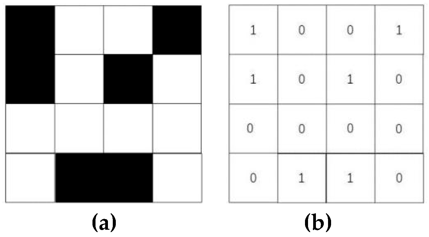
Figure 2.
Schematic illustration of population hierarchy division.
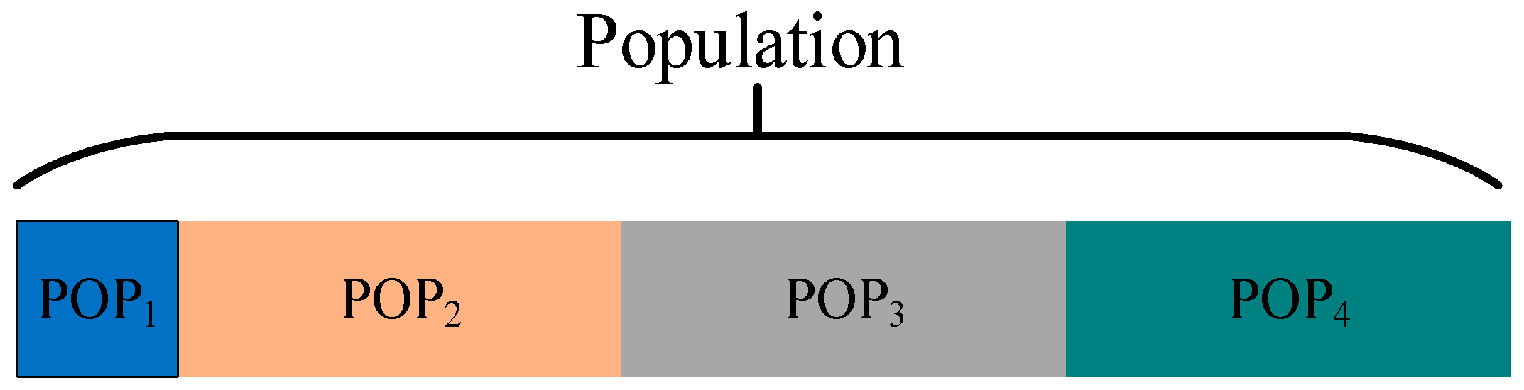
Figure 3.
Strong perturbation operation.
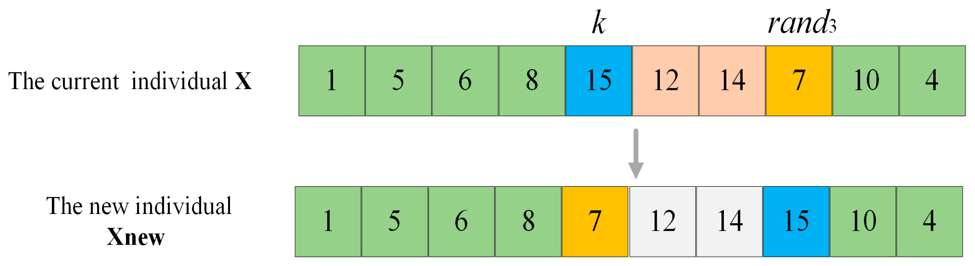
Figure 4.
Weak perturbation operation.
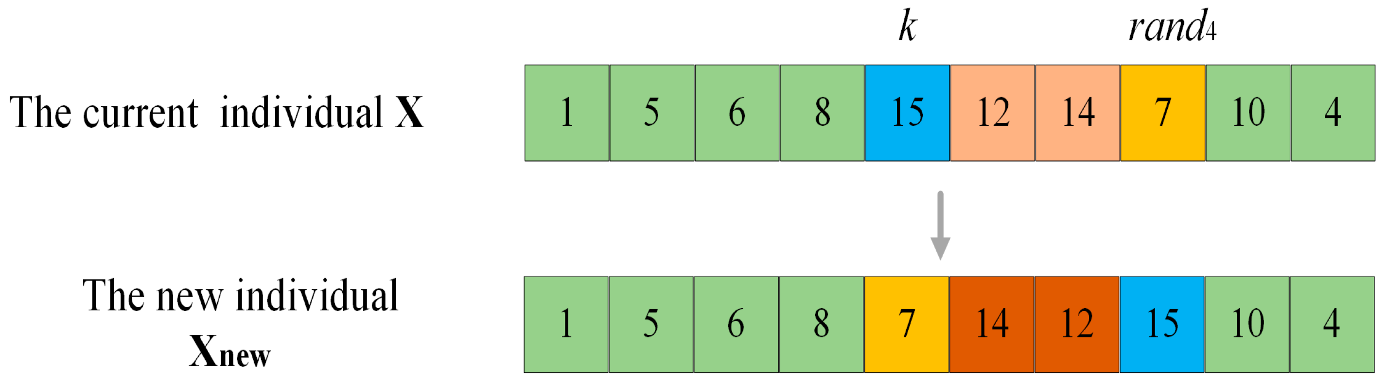
Figure 5.
Learning operation.
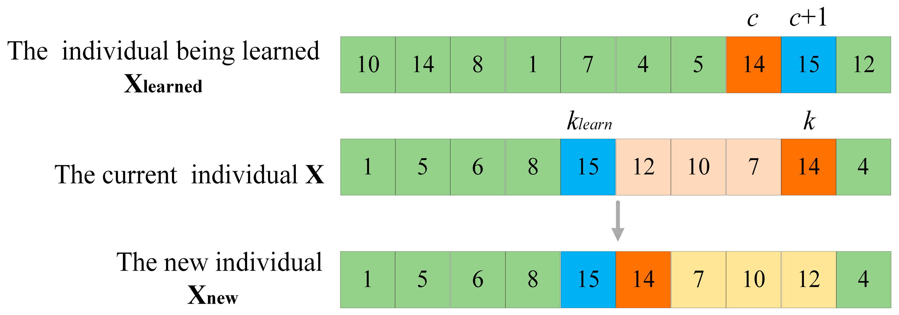
Figure 6.
Initial paths generated by the three strategies. (a) Random initialization strategy. (b) Initialization strategy of ACO. (c) Greedy initialization strategy based on transition probability.
Figure 6.
Initial paths generated by the three strategies. (a) Random initialization strategy. (b) Initialization strategy of ACO. (c) Greedy initialization strategy based on transition probability.
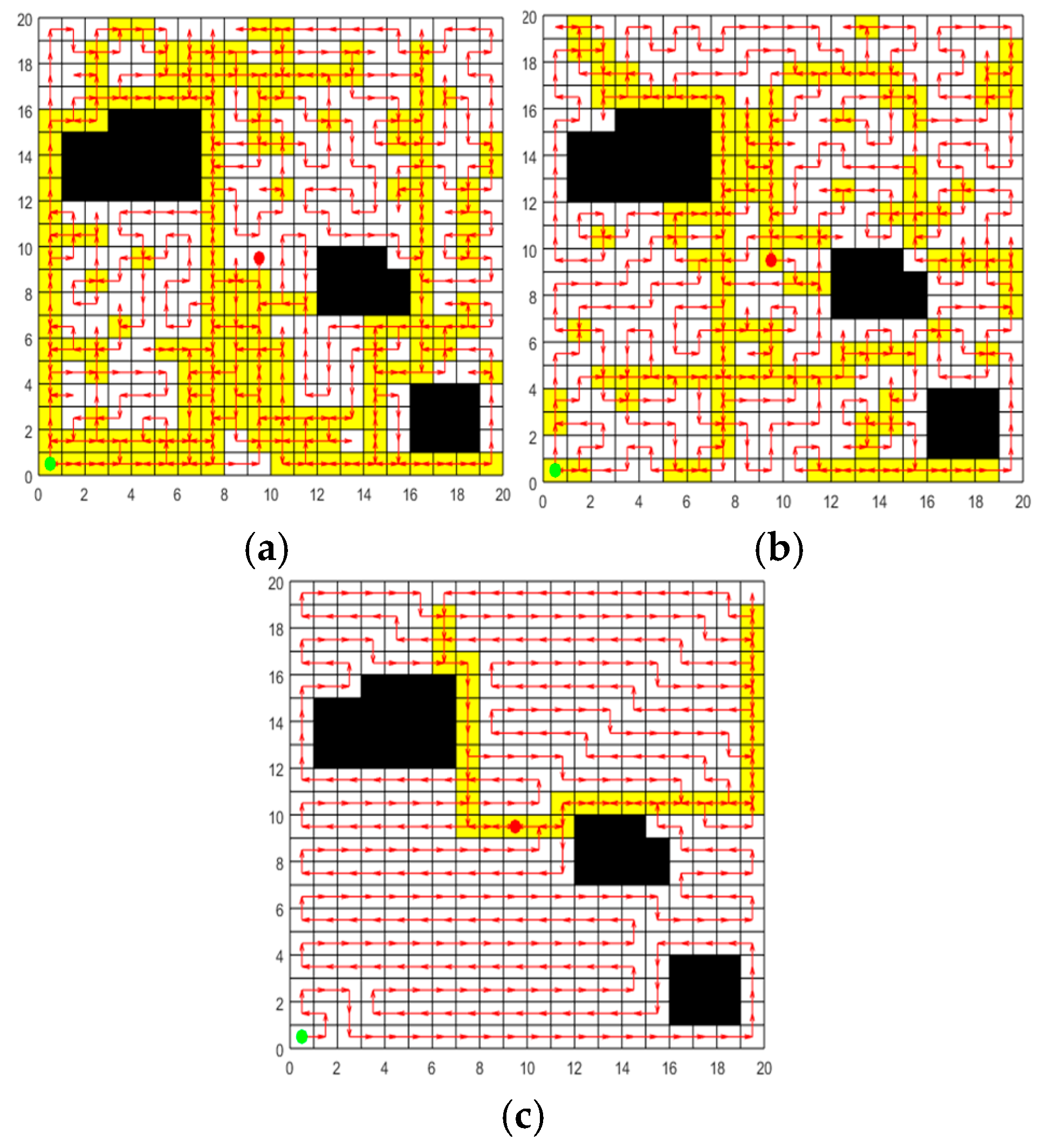
Figure 7.
Optimal paths obtained by the three strategies. (a)The update strategy of ACO. (b)The update strategy of SPBO. (c)The update strategy of learning perturbation.
Figure 7.
Optimal paths obtained by the three strategies. (a)The update strategy of ACO. (b)The update strategy of SPBO. (c)The update strategy of learning perturbation.
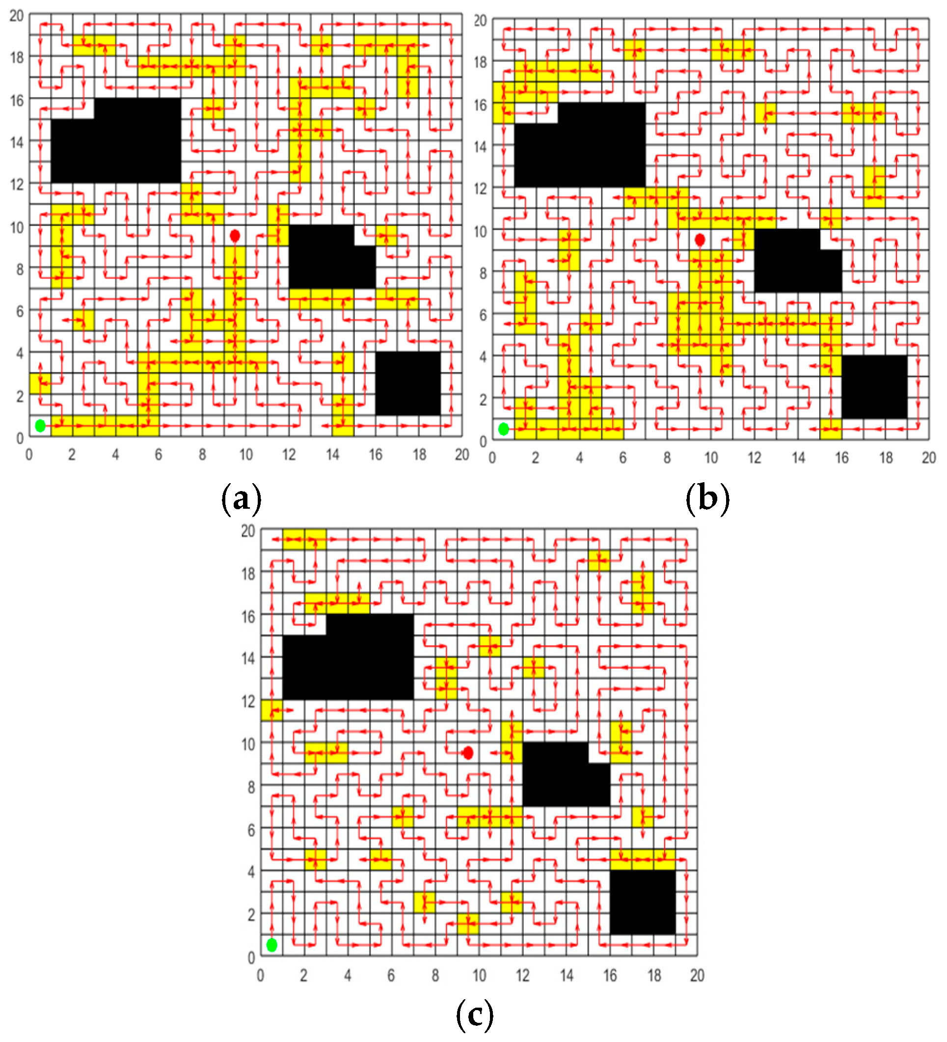
Figure 8.
The schematic diagrams of four maps. (a)Environment I. (b)Environment II. (c)Environment III. (d)Environment IV.
Figure 8.
The schematic diagrams of four maps. (a)Environment I. (b)Environment II. (c)Environment III. (d)Environment IV.
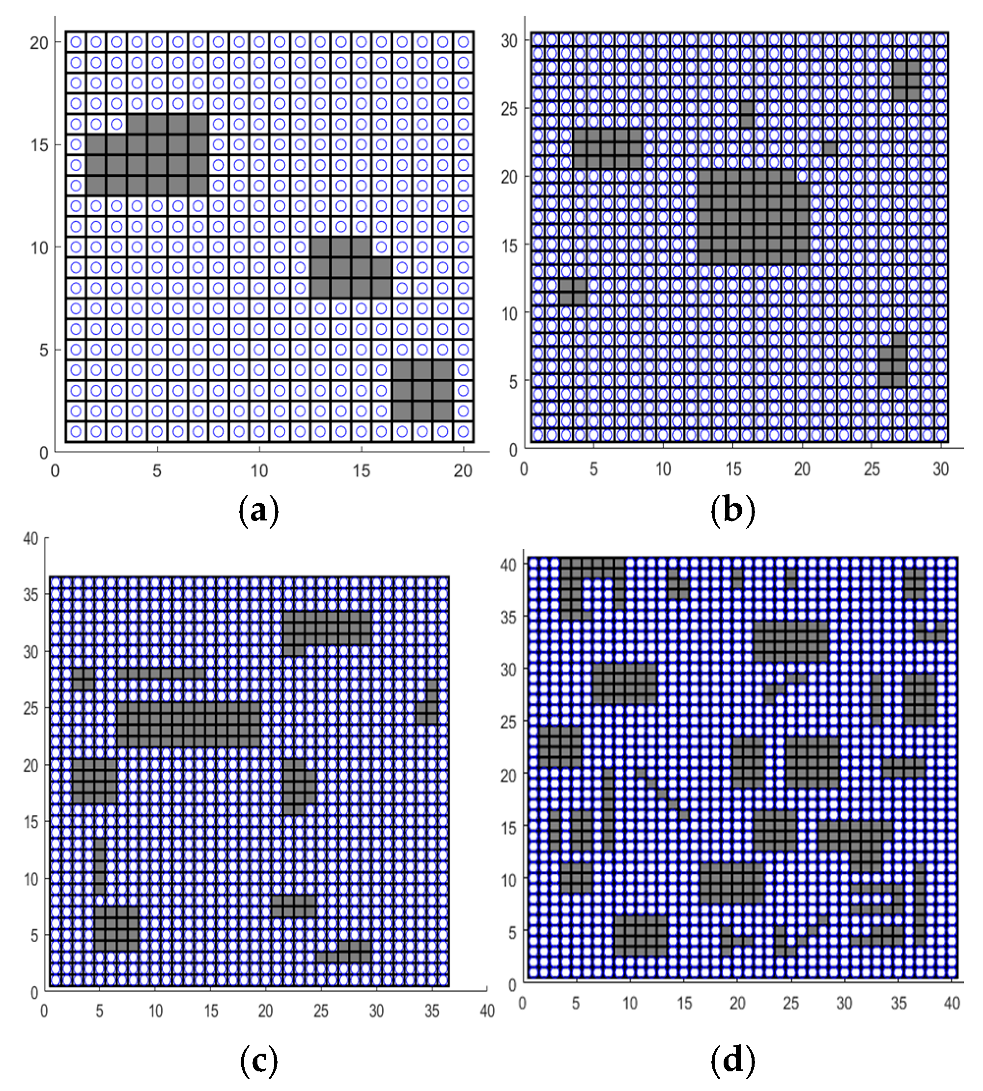
Figure 9.
Optimal path obtained by each algorithm in environment I. (a) Optimal path of ACO. (b) Optimal path of GWO. (c) Optimal path of SPBO (d) Optimal path of DJAYA. (e) Optimal path of DTSA. (f) Optimal path of CCPP-TPLP.
Figure 9.
Optimal path obtained by each algorithm in environment I. (a) Optimal path of ACO. (b) Optimal path of GWO. (c) Optimal path of SPBO (d) Optimal path of DJAYA. (e) Optimal path of DTSA. (f) Optimal path of CCPP-TPLP.
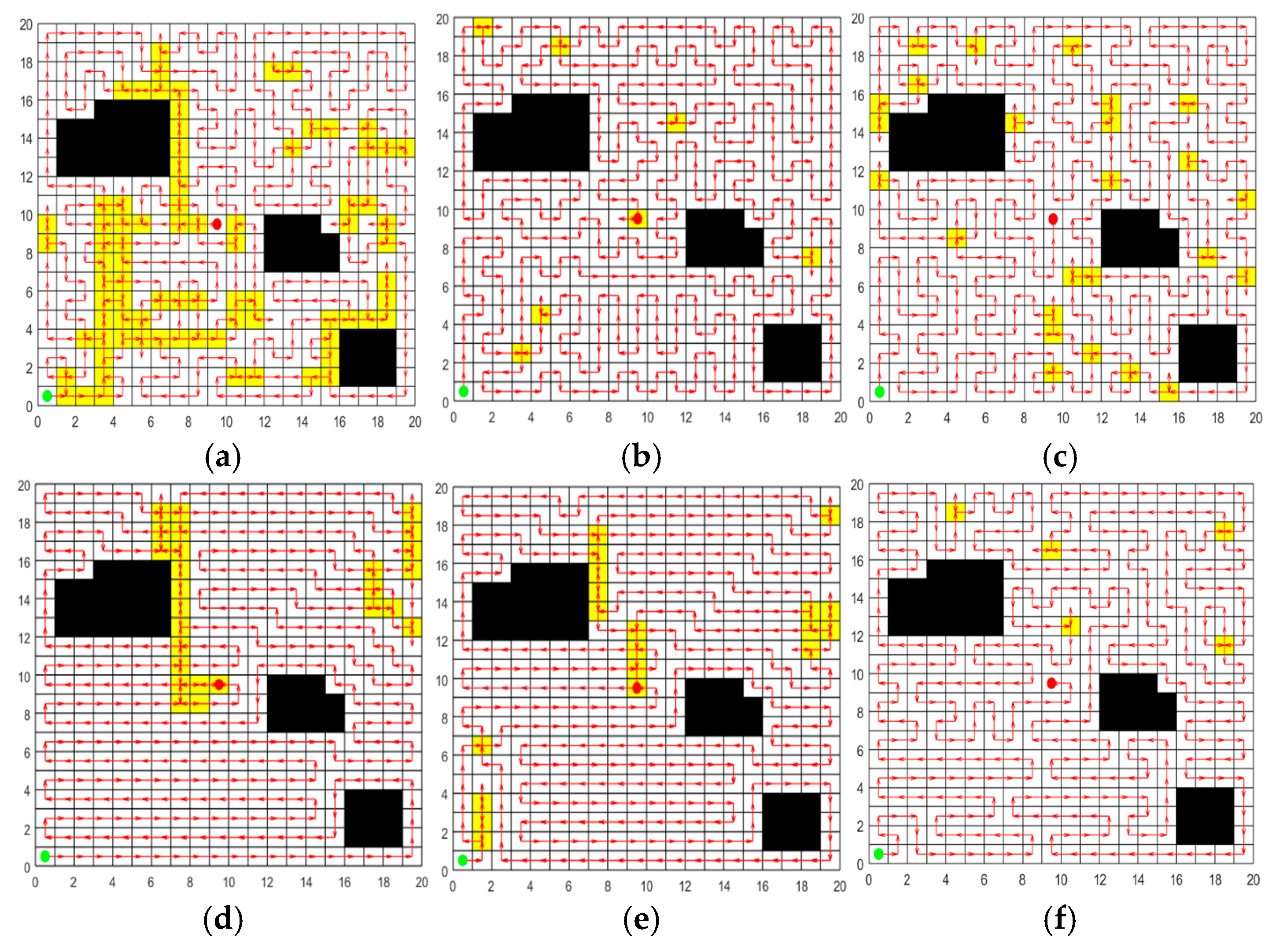
Figure 10.
Optimal path obtained by each algorithm in environment II. (a) Optimal path of ACO. (b) Optimal path of GWO. (c) Optimal path of SPBO. (d) Optimal path of DJAYA. (e) Optimal path of DTSA. (f) Optimal path of CCPP-TPLP.
Figure 10.
Optimal path obtained by each algorithm in environment II. (a) Optimal path of ACO. (b) Optimal path of GWO. (c) Optimal path of SPBO. (d) Optimal path of DJAYA. (e) Optimal path of DTSA. (f) Optimal path of CCPP-TPLP.
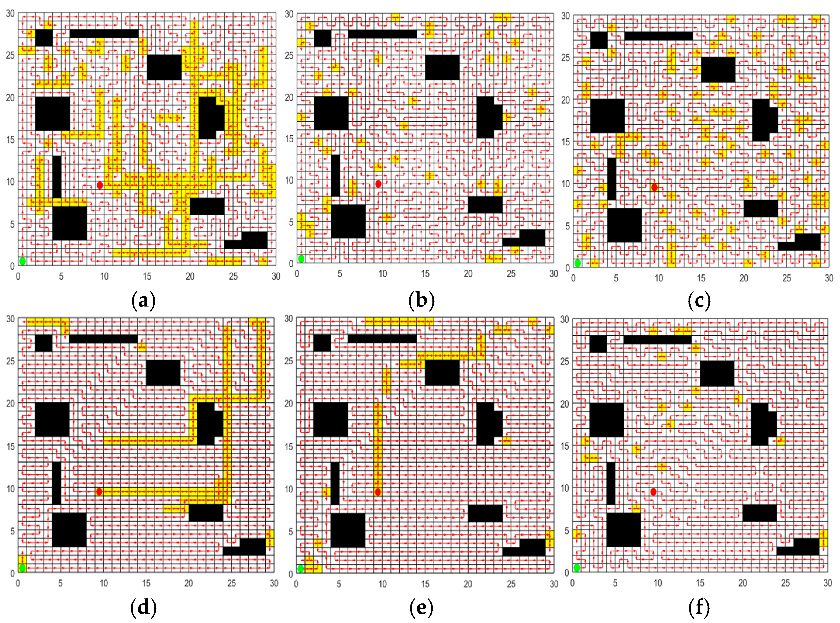
Figure 11.
Optimal path obtained by each algorithm in environment III. (a) Optimal path of ACO. (b) Optimal path of GWO. (c) Optimal path of SPBO. (d) Optimal path of DJAYA. (e) Optimal path of DTSA. (f) Optimal path of CCPP-TPLP.
Figure 11.
Optimal path obtained by each algorithm in environment III. (a) Optimal path of ACO. (b) Optimal path of GWO. (c) Optimal path of SPBO. (d) Optimal path of DJAYA. (e) Optimal path of DTSA. (f) Optimal path of CCPP-TPLP.
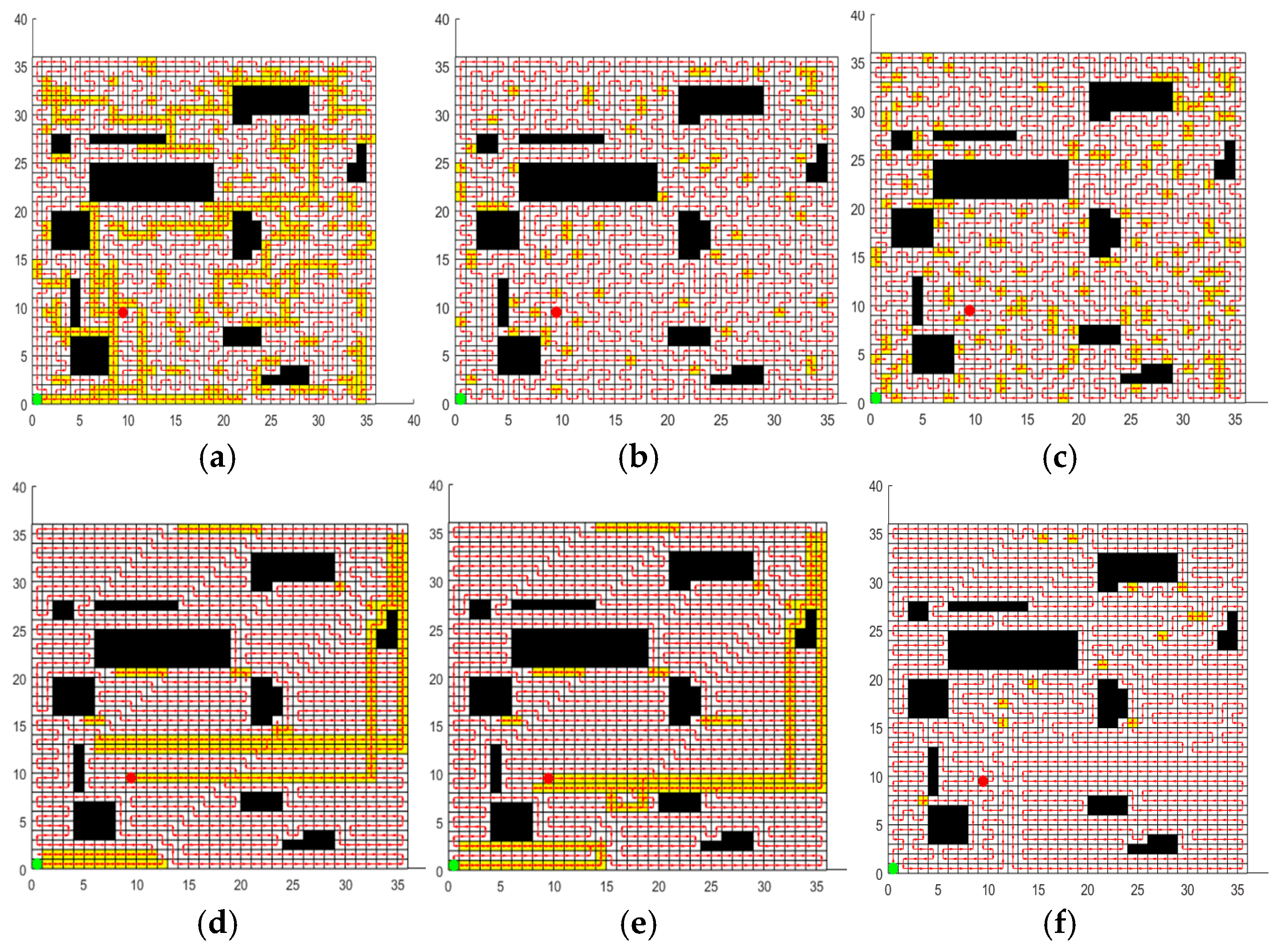
Figure 12.
Optimal path obtained by each algorithm in environment IV. (a) Optimal path of ACO. (b) Optimal path of GWO. (c) Optimal path of SPBO. (d) Optimal path of DJAYA. (e) Optimal path of DTSA. (f) Optimal path of CCPP-TPLP.
Figure 12.
Optimal path obtained by each algorithm in environment IV. (a) Optimal path of ACO. (b) Optimal path of GWO. (c) Optimal path of SPBO. (d) Optimal path of DJAYA. (e) Optimal path of DTSA. (f) Optimal path of CCPP-TPLP.
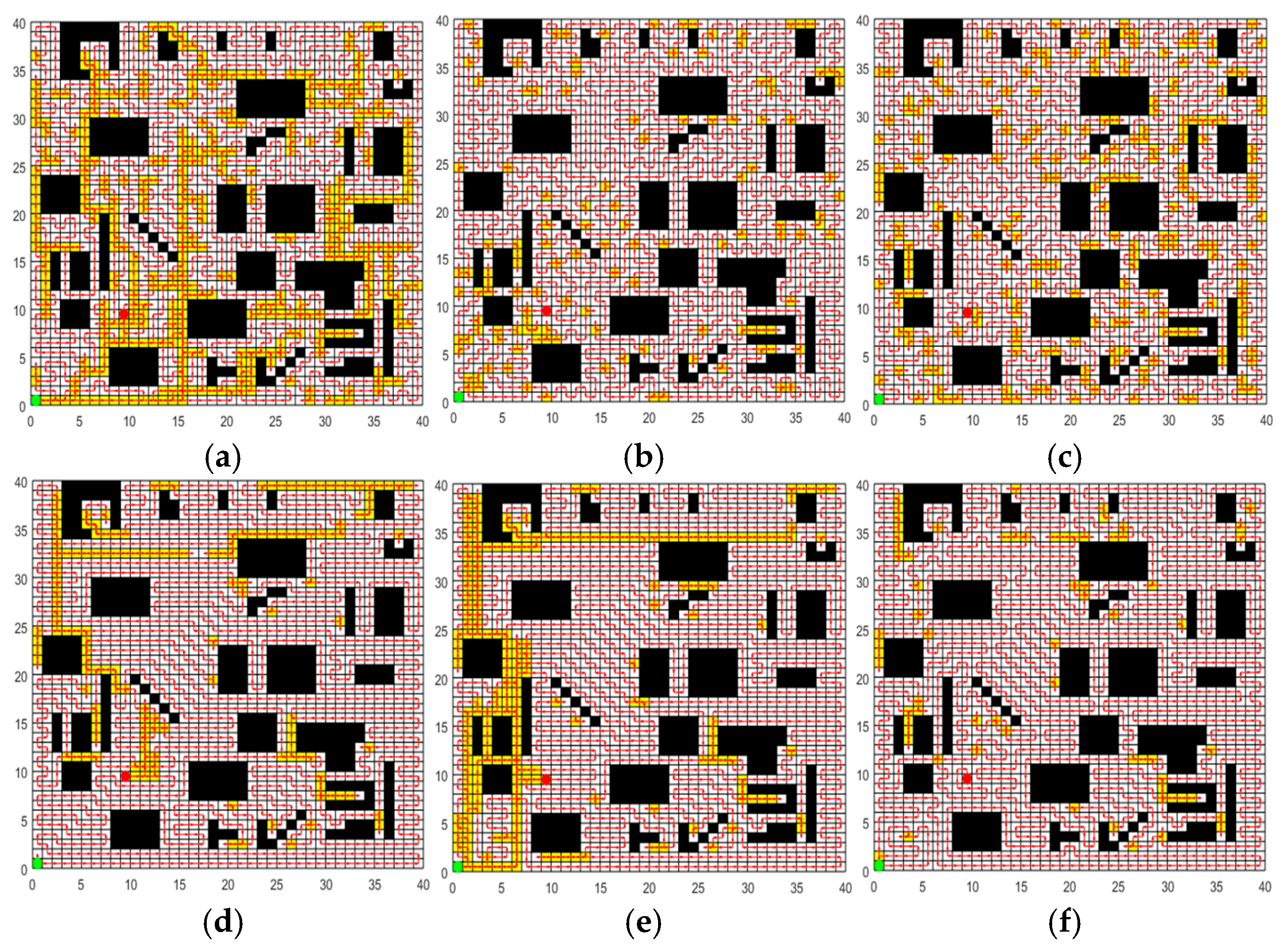
Figure 13.
Convergence curves of each algorithm in four map environments. (a) Environment I. (b) Environment II. (c) Environment III. (d) Environment IV.
Figure 13.
Convergence curves of each algorithm in four map environments. (a) Environment I. (b) Environment II. (c) Environment III. (d) Environment IV.
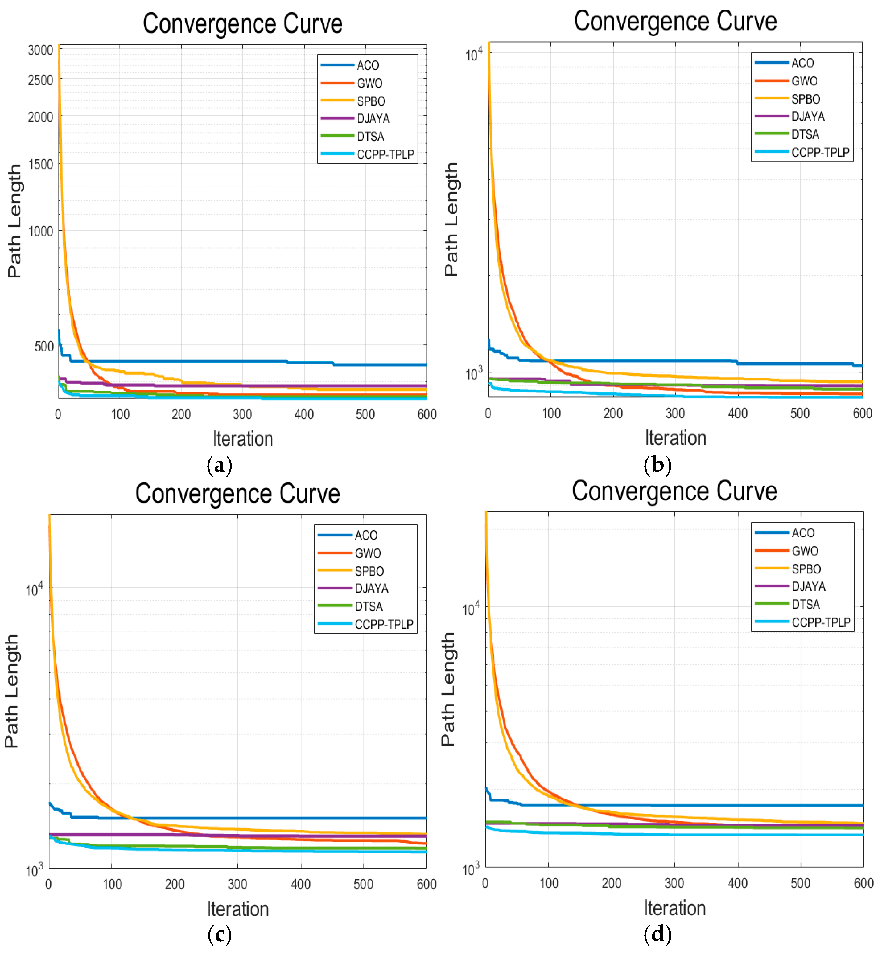
Figure 14.
Height information of the map.
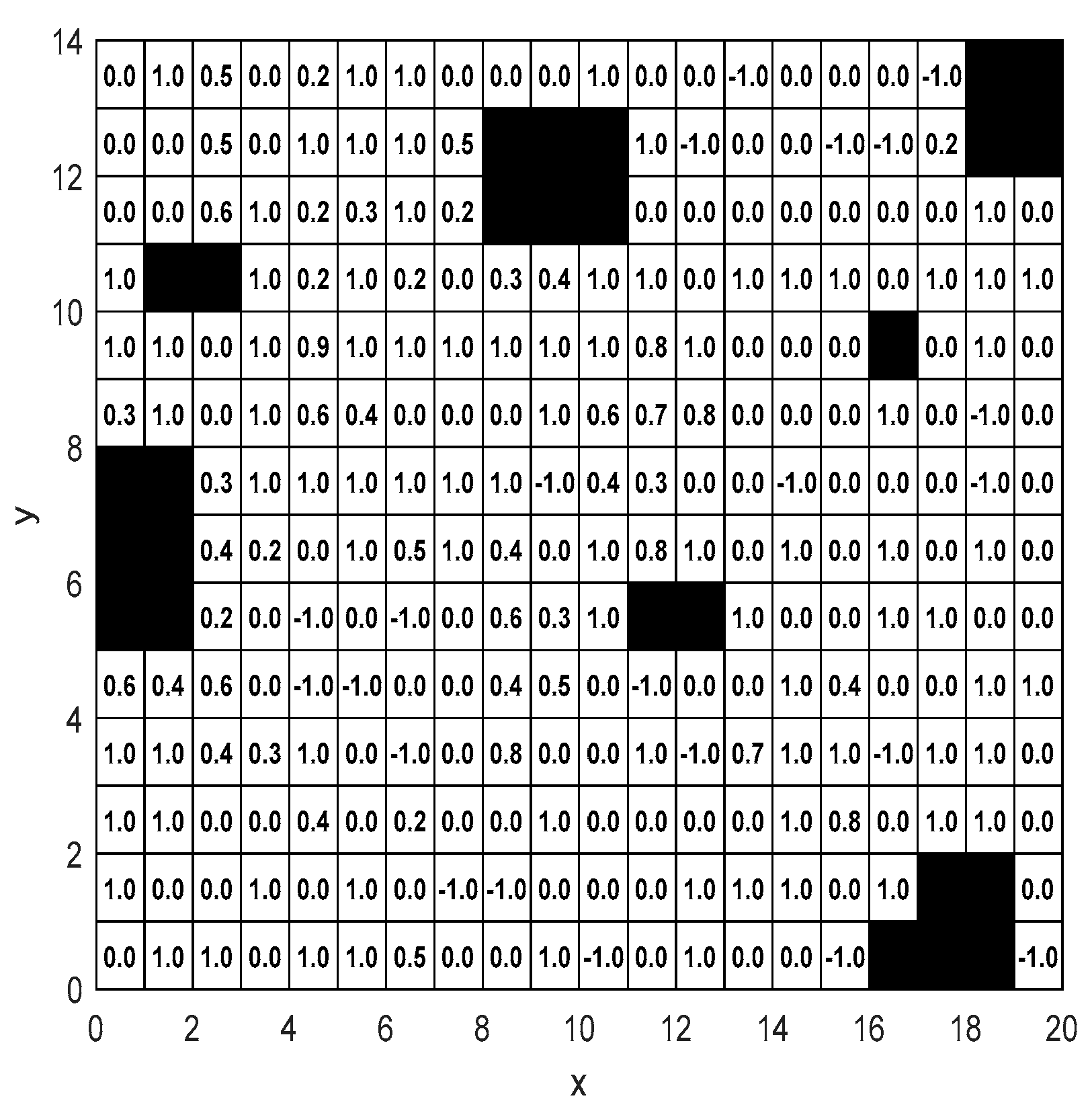
Figure 15.
Optimal path obtained by each algorithm in the tractor working map. (a) Optimal path of ACO. (b) Optimal path of GWO. (c) Optimal path of SPBO. (d) Optimal path of DJAYA. (e) Optimal path of DTSA. (f) Optimal path of CCPP-TPLP.
Figure 15.
Optimal path obtained by each algorithm in the tractor working map. (a) Optimal path of ACO. (b) Optimal path of GWO. (c) Optimal path of SPBO. (d) Optimal path of DJAYA. (e) Optimal path of DTSA. (f) Optimal path of CCPP-TPLP.
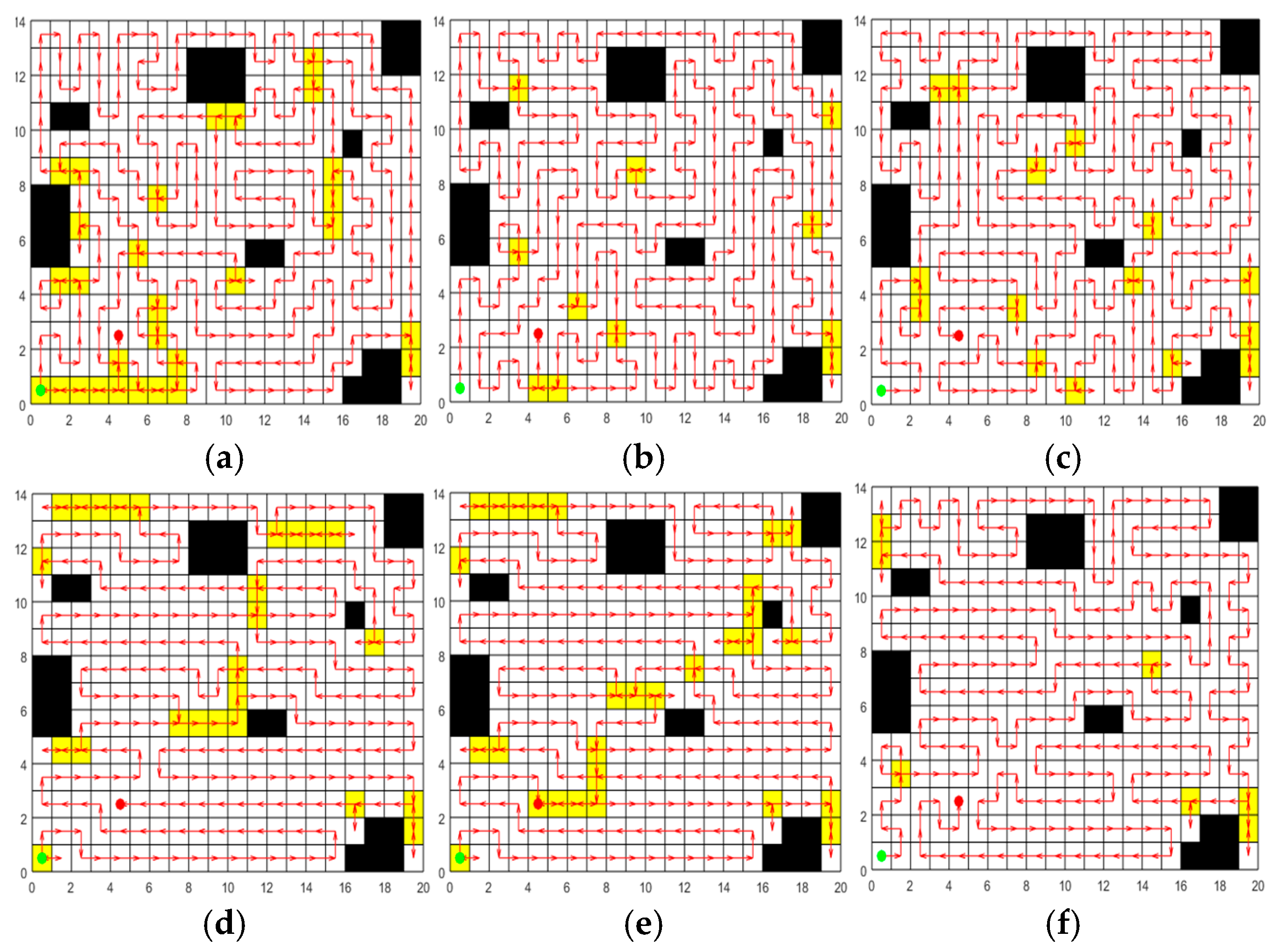

Table 1.
Parameter settings of the comparison algorithms.
| Algorithm | Parameter setting |
| ACO | The pheromone heuristic factor α is 1, the distance heuristic factor β is 5, the pheromone heuristic factor is 0.1, and the pheromone enhancement factor is 100 |
| GWO | The convergence factor a decreases linearly from 2 to 0 |
| SPBO | The ratio of population distribution is 1:1:1:1 |
| DJAVA | ST1=0.5, ST2=0.5, the probability of swap transformation swap=0.2, the probability of shift transformation shift=0.5, the probability of symmetry transformation symmetry= 0.3 |
| DTSA | ST1=0.5, ST2=0.5, the probability of swap transformation swap=0.2, the probability of shift transformation shift=0.5, the probability of symmetry transformation symmetry= 0.3 |
Table 2.
Results of initial paths of the three strategies.
| Strategy | Path length | ||||
| Mean | Std. | Mean | Std. | ||
| Random initialization strategy | 100% | 47.54% | 0.036 | 4606.70 | 54.935 |
| Initialization strategy of ACO | 100% | 37.57% | 0.023 | 529.50 | 14.795 |
| Greedy initialization strategy based on transition probability | 100% | 9.99% | 0.008 | 418.60 | 7.950 |
Table 3.
Statistical results of population updated by the three strategies.
| Strategy | Path length | ||||
| Mean | Std. | Mean | Std. | ||
| ACO | 100% | 22.99% | 0.017 | 451.20 | 4.467 |
| SPBO | 100% | 22.04% | 0.021 | 441.80 | 7.194 |
| Learning perturbation operation | 100% | 10.60% | 0.011 | 395.30 | 4.219 |
Table 4.
The experimental results of different greedy factor when =1.
| Path length | |||||
| Mean | Std. | Mean | Std. | ||
| 0.1 | 100% | 4.30% | 0.015 | 372.40 | 5.317 |
| 0.5 | 100% | 4.39% | 0.012 | 372.80 | 4.341 |
| 1 | 100% | 4.42% | 0.007 | 372.20 | 2.743 |
| 2 | 100% | 3.85% | 0.013 | 371.40 | 4.812 |
| 5 | 100% | 3.29% | 0.006 | 368.80 | 2.348 |
| 10 | 100% | 3.91% | 0.011 | 371.20 | 4.341 |
| 20 | 100% | 3.77% | 0.011 | 370.60 | 2.503 |
| 50 | 100% | 3.88% | 0.012 | 371.00 | 4.028 |
Table 5.
The experimental results of different degree of greediness when =5.
| Path length | |||||
| Mean | Std. | Mean | Std. | ||
| 0.5 | 100% | 7.21% | 0.017 | 383.20 | 5.750 |
| 0.6 | 100% | 6.56% | 0.015 | 381.40 | 5.502 |
| 0.7 | 100% | 6.68% | 0.016 | 381.00 | 5.598 |
| 0.8 | 100% | 5.31% | 0.009 | 376.00 | 3.399 |
| 0.9 | 100% | 4.41% | 0.013 | 372.80 | 4.733 |
| 1 | 100% | 3.30% | 0.006 | 368.80 | 2.348 |
Table 6.
Experimental results under different division ratios.
| Division Ratio | Path length | ||||
| Mean | Std. | Mean | Std. | ||
| 0.5:1.5:3 | 100% | 2.63% | 0.009 | 366.20 | 3.327 |
| 1:1:1 | 100% | 2.46% | 0.007 | 365.80 | 2.394 |
| 1:2:1 | 100% | 2.51% | 0.007 | 366.00 | 2.494 |
| 1:2:2 | 100% | 1.84% | 0.006 | 363.60 | 2.271 |
| 2:1:1 | 100% | 1.62% | 0.008 | 372.80 | 4.341 |
| 2:1:2 | 100% | 1.62% | 0.009 | 362.80 | 3.327 |
| 2:2:1 | 100% | 1.50% | 0.008 | 362.40 | 2.836 |
| 2.5:1.5:1 | 100% | 2.49% | 0.012 | 366.00 | 4.320 |
Table 7.
Parameters of four map environments.
| Map environment | Map size | Proportion of accessible Area | Quantity of discrete obstacles |
| Environment I | 20m*20m | 89.50% | 3 |
| Environment II | 30m*30m | 90.00% | 7 |
| Environment III | 36m*36m | 87.50% | 11 |
| Environment IV | 40m*40m | 81.56% | 29 |
Table 8.
Experimental results of each algorithm in four map environments.
| Map Environment | Algorithm | Path length | Convergence iteration | ||||
| Mean | Std. | Mean | Std. | Mean | |||
| Environment I | ACO | 100% | 19.05% | 0.032 | 435.60 | 12.322 | 433.40 |
| GWO | 100% | 3.93% | 0.014 | 371.40 | 5.064 | 494.40 | |
| SPBO | 100% | 8.10% | 0.016 | 386.00 | 5.586 | 567.00 | |
| DJAYA | 100% | 11.98% | 0.025 | 391.20 | 12.218 | 457.40 | |
| DTSA | 100% | 6.96% | 0.021 | 371.80 | 4.050 | 398.90 | |
| CCPP-TPLP | 100% | 2.79% | 0.007 | 367.00 | 2.366 | 312.30 | |
| Environment II | ACO | 100% | 25.90% | 0.028 | 1044.60 | 19.323 | 280.90 |
| GWO | 100% | 6.16% | 0.011 | 859.80 | 10.042 | 543.80 | |
| SPBO | 100% | 11.85% | 0.012 | 906.00 | 10.284 | 572.80 | |
| DJAYA | 100% | 11.56% | 0.018 | 896.50 | 18.368 | 495.60 | |
| DTSA | 100% | 8.75% | 0.021 | 882.60 | 17.640 | 507.80 | |
| CCPP-TPLP | 100% | 2.91% | 0.005 | 832.60 | 4.115 | 457.50 | |
| Environment III | ACO | 100% | 28.29% | 0.008 | 1505.80 | 11.980 | 275.70 |
| GWO | 100% | 7.18% | 0.015 | 1217.80 | 19.966 | 559.00 | |
| SPBO | 100% | 11.85% | 0.012 | 906.00 | 10.284 | 568.80 | |
| DJAYA | 100% | 11.56% | 0.018 | 896.50 | 18.368 | 472.10 | |
| DTSA | 100% | 8.75% | 0.021 | 882.60 | 17.640 | 500.90 | |
| CCPP-TPLP | 100% | 2.91% | 0.005 | 832.60 | 4.115 | 456.60 | |
| Environment IV | ACO | 100% | 28.74% | 0.012 | 1710.60 | 9.800 | 503.50 |
| GWO | 100% | 10.02% | 0.060 | 1393.46 | 16.400 | 580.20 | |
| SPBO | 100% | 16.91% | 0.010 | 1479.40 | 13.500 | 592.10 | |
| DJAYA | 100% | 13.56% | 0.016 | 1447.50 | 21.246 | 434.60 | |
| DTSA | 100% | 11.82% | 0.008 | 1403.90 | 19.445 | 550.20 | |
| CCPP-TPLP | 100% | 5.67% | 0.005 | 1330.20 | 7.083 | 510.90 | |
Table 9.
Experimental results of each algorithm in the tractor operation environment map.
| Algorithm | Path length | Fitness value | |||||
| Mean | Std. | Mean | Std. | Mean | Std. | ||
| ACO | 100% | 17.65% | 0.029 | 302.50 | 6.771 | 3.777*10-3 | 7.225*10-5 |
| GWO | 100% | 5.79% | 0.013 | 267.70 | 3.389 | 3.951*10-3 | 7.323*10-5 |
| SPBO | 100% | 7.18% | 0.015 | 273.80 | 3.833 | 3.876*10-3 | 6.854*10-5 |
| DJAYA | 100% | 21.44% | 0.049 | 288.30 | 10.183 | 4.070*10-3 | 1.986*10-5 |
| DTSA | 100% | 15.22% | 0.031 | 293.90 | 8.813 | 4.135*10-3 | 8.124*10-5 |
| CCPP-TPLP | 100% | 4.74% | 0.009 | 265.90 | 2.382 | 4.155*10-3 | 3.091*10-5 |
Disclaimer/Publisher’s Note: The statements, opinions and data contained in all publications are solely those of the individual author(s) and contributor(s) and not of MDPI and/or the editor(s). MDPI and/or the editor(s) disclaim responsibility for any injury to people or property resulting from any ideas, methods, instructions or products referred to in the content. |
© 2025 by the authors. Licensee MDPI, Basel, Switzerland. This article is an open access article distributed under the terms and conditions of the Creative Commons Attribution (CC BY) license (http://creativecommons.org/licenses/by/4.0/).
Copyright: This open access article is published under a Creative Commons CC BY 4.0 license, which permit the free download, distribution, and reuse, provided that the author and preprint are cited in any reuse.


