
Submitted:
01 April 2025
Posted:
01 April 2025
You are already at the latest version
Abstract
In operational testing contexts, testers face dual challenges of constrained timeframes and limited resources, both of which impede the generation of reliability test data. To address this issue, integrating data from similar systems with test data can effectively expand data sources. This study proposes a systematic approach wherein the mission of the system under test (SUT) is decomposed to identify candidate subsystems for data combination. A phylogenetic tree representation is constructed for subsystem analysis and subsequently mapped to a mixed integer programming (MIP) model, enabling efficient computation of similarity factors. A reliability assessment model that combines data from similar subsystems is established. The similarity factor is regarded as a covariate, and the regression relationship between it and the subsystem failure time distribution is established. Leveraging Bayesian theory, the joint posterior distribution of regression coefficients is derived. These coefficients are then sampled via the No-U-Turn Sampler (NUTS) algorithm to obtain reliability estimates. Numerical case studies demonstrate that the proposed method outperforms existing approaches, yielding more robust similarity factors and higher accuracy in reliability assessments.
Keywords:
operational test
; reliability assessment
; Bayesian theory
; similarity factor
1. Introduction
Reliability assessment serves as a critical element in equipment test and evaluation, forming an integral component of general quality characteristic assessment. This evaluation dimension maintains inherent connections with maintainability, supportability, and availability analyses, collectively determining operational suitability of equipment systems [1]. While reliability metrics such as Mean Time Between Failure (MTBF), mission reliability, and mean flight hours between failure vary across systems under test (SUT), their assessment remains fundamental to system validation.
Traditional reliability assessment methodologies typically require extensive failure datasets, presenting significant challenges in operational testing contexts. Unlike dedicated reliability trials, operational tests prioritize mission-specific evaluations within constrained timeframes and resource allocations [2]. Consequently, the reliability assessment objectives in operational testing have shifted from comprehensive performance mapping to maximizing evaluation effectiveness under specific mission [3]. This paradigm necessitates developing optimized test strategies that balance data availability with assessment rigor, particularly crucial for time-sensitive procurement programs facing compressed testing schedules [4].
Advances in data collection and storage technologies have expanded potential data sources for reliability assessment beyond conventional field tests. Current approaches increasingly incorporate historical failure data from analogous systems, performance metrics, and expert knowledge to complement operational test data. Among these supplementary sources, data from similar systems proves particularly valuable due to inherent design commonalities in modern equipment development. Modular architectures and evolutionary design practices often create structural, functional, and operational similarities between SUTs and previous-generation systems, both within product families and across different lineages [5].
Effective utilization of similar system data for reliability assessment necessitates addressing two critical challenges: (1) quantifying similarity metrics between reference systems and the SUT, and (2) developing appropriate reliability modeling frameworks. Current similarity quantification methods predominantly employ statistical techniques like grey correlation analysis [6], Pearson’s correlation coefficient [7], Mahalanobis distance [8], Euclidean distance [9], and included angle cosine [10]. However, these approaches require substantial datasets and demonstrate limited efficacy under sparse data conditions. Inheritance factor methodologies attempt to identify common system elements through expert-driven value assignment [11], though subjective bias remains a concern. Regarding model development, the similar product method can elucidate the influence of environmental and derating factors on system failure rates, thereby establishing a correlation between the failure rates of similar systems [12]. However, this approach does not allow for the full utilization of the system’s reliability data. By integrating the system development mechanism and physical parameter analysis, the life equivalence method can equalize the failure time of similar systems [13]. It is essential that the evaluator possess a comprehensive understanding of the system’s operational mechanism and physical characteristics. The application of fuzzy theory [14] and evidence theory [15] introduce non-probabilistic theory into the data analysis process of similar systems. Bayesian theory [16] is a widely utilized approach in the data analysis of similar systems. It employs a prior distribution to express the information of similar systems, combines the data of the SUT via the inheritance factor, or combines different prior distributions with the data model of the SUT, respectively, and then combines the evaluation results to form a comprehensive conclusion [17]. However, the calculation process of this method contains some expressions of complex forms that are difficult to solve, which presents a challenge in practical applications.
To address these limitations in operational testing scenarios, this paper puts forth a methodology for the combination of data from similar subsystems with the aim of conducting a reliability assessment for subsystem under test (SSUT). The methodology encompasses three phases: (1) Mission decomposition using hierarchical method to identify Mission Essential Functions (MEFs) and corresponding subsystems, (2) Phylogenetic Tree (PT) representation of subsystem Bill of Materials (BOM) with environmental considerations, followed by Mixed Integer Programming (MIP)-based similarity factor computation, and (3) Bayesian reliability modeling incorporating similarity covariates, with posterior distribution sampling via Markov Chain Monte Carlo (MCMC) techniques. The No-U-Turn Sampler (NUTS) algorithm enables efficient sampling from the posterior distributions. The following is a presentation of three innovations contained in this article.
(1) The impact of subsystem configuration and external circumstances on the reliability of basic components is taken into account in the similarity factor calculation methodology. PT is employed to illustrate the subsystem structure, the process of calculating the distance between subsystems is subjected to rigorous analysis, and MIP is utilized to facilitate the expeditious resolution of the similarity factor.
(2) A reasonable reliability assessment model is established, incorporating similarity factors, failure data, and regression coefficient priors. The NUTS-enhanced MCMC sampling ensures robust posterior estimation.
(3) Implements system mission decomposition to establish precise data combination targets, aligning with operational test requirements.
The subsequent sections are organized as follows: Section 2 presents the mission decomposition framework for identifying subsystems requiring data combination. Section 3 details the calculation process of similarity factor, including the construction of PT representation, the calculation of distance, and the application of MIP. Section 4 describes the reliability assessment model. Section 5 serves to validate the proposed methodology and demonstrate its superiority over existing techniques through the presentation of two illustrative examples. Section 6 briefly summarizes the entire paper and draws some conclusions.
2. Hierarchical Decomposition of the SUT’s Mission
In operational test, SUT is required to perform the designated test activities in accordance with the mission profile, which delineates the SUT’s tasks, activities, frequencies, periods, environmental conditions, and operational contexts at each stage. Additionally, the mission profile specifies the operational activities and environmental conditions pertinent to specific tasks, organized according to a timeline [18]. Therefore, the SUT in this context can be considered as a Phased-Mission-System (PMS), which may have different functional structures in different mission phases, requiring different subsystems to perform different MEFs, where MEF refers to the minimum set of functions that must be performed to accomplish the specified operational tasks [19]. The SUT in operational test is given one or more missions to describe the critical tasks that must be accomplished to meet the user’s needs. The aim of the mission is explicit, while the specific ways of accomplishing the mission need not be explicit. For example, a certain type of carrier-based aircraft is required to provide close air fire support for a ship formation. If there is insufficient test data for the SUT and other data sources must be found, it is not possible to measure similarity for the entire system, because only certain subsystems or components may be similar between the SUT and the comparison system. As an illustration, the reliability of the 57-mm gun on the Littoral Combat Ship (LCS) can be assessed by combining the 57-mm gun test data from the National Security Cutter (NSC). Despite the fact that it may have been modified to fit different platforms, there are still considerable areas of commonality. The mission of the SUT is decomposed hierarchically into MEFs, which are then mapped to the subsystems. By comparing the mission profile with the decomposition structure, the subsystems involved in operational test can be clearly presented, thus allowing the similarity factors between different subsystems to be targeted. The tree structure of mission decomposition is illustrated in Figure 1.
As illustrated in Figure 1, the mission of SUT is structured in accordance with the missiontasksubtaskmetataskMEF hierarchy, with a corresponding relationship between the MEFs and the subsystems. Furthermore, subtasks may also exist at multiple levels, and metatask is the task that do not necessitate further decomposition at a specific level of granularity. In operational tests, due to the characteristics of the PMS, the object of data combination is subsystem.
3. Similarity Factor Calculation
This section provides a detailed account of the methodology employed in calculating the similarity factor. It begins by outlining the process of establishing a PT representation of the subsystem. This is followed by a description of the approach used to calculate distance, taking into account the external circumstance. The subsequent step is to present the MIP solution for calculating distance and deriving the similarity factor.
3.1. Establishment of PT Representation
The calculation of similarity factor requires the establishment of a suitable representation model to quantify the relevant elements. In addition to its application in the field of reliability assessment, similarity analysis has also been the subject of considerable interest among experts and scholars in the domains of design and manufacturing. Group technology [20] represents a traditional methodology for the analysis of product similarity. However, it necessitates a considerable investment of effort to ensure the continual refinement of the coding system. Similarity analysis based on functional features has also been developed in the field of design retrieval [21]. The challenge in applying it lies in the representation of codes for identifying functional features and the calculation of similarity based on functional feature ranking. Following years of practice and investigation, it has become evident that reliability is contingent upon the design, is refined during production, and is manifested in use [22]. The product structure can be conceptualized as a form of data that is shaped during the extended design and manufacturing process, reflecting the composition and interrelationships of the product’s internal components. Consequently, the product structure is inextricably linked to the reliability level, and research into its similarities has also garnered significant interest [23].
BOM was originally proposed by Dr. Orlicky [24] as a form of product data structure subordinate to the Material Requirements Planning (MRP) system commonly used for production planning and inventory control. BOM is a list of components, raw materials and their quantities required to produce the final product, which can be represented by an unordered root tree. Literatures [25,26,27] employ BOM-based similarity metrics to ascertain the similarity between products. However, factors such as material composition, test circumstance, and operator level may influence product reliability data and thus warrant further investigation.
Figure 2 illustrates the BOM tree structure of two three-level subsystems, comprising eight and seven distinct basic components (numbered 8,9,5,2,6,10,11,12), respectively. The number adjacent to each component indicates the quantity required to form a parent component. For instance, component 1 is the parent of component 4 in T1, and three component 4 are necessary to produce one component 1. Figure 2 is merely an illustrative example, and the actual scenario may encompass a greater number of components and hierarchies.
A BOM tree can be transformed into a PT, thereby facilitating the calculation of similarity factors. PT, also referred to as molecular evolutionary tree, is a method utilized in bioinformatics for the classification of a group of species that have descended from a common ancestor, as well as for the study of their evolutionary history [28]. Figure 3 depicts two PTs corresponding to Figure 2. The arbitrarily ordered numbers “①②③④⑤” indicate nodes, and the number of components associated with each node is shown in parentheses adjacent to the basic components.
3.2. Distance Calculation Principle
Robinson-Foulds (RF) distance is a widely utilized metric for comparing PTs [29]. However, it is unable to account for quantitative differences between nodes and components. This limitation can be addressed by performing a bijective mapping between the subsystems [26]. Taking the PTs in Figure 3 as an example, each node in T1 is mapped to the most similar node in T2, and this process is repeated for each node in T2. The resulting mapping distances are then summarized in Table 1 and Table 2.
In Table 1, column 1 contains all the nodes in T1, and column 2 contains the nodes in T2 that are most similar to the nodes in column 1. This can be determined visually in simple PTs. Column 3 shows the components that are present in T1 but not in T2. Column 4 enumerates the components that are more in T1 than in T2, among those that are shared by the corresponding nodes. Column 5 contains the hierarchical level differences between the components contained in columns 3~4 and the corresponding nodes. For example, if node ① is marked at level 0, then components 6, 10, and 11 are, in turn, marked at level 2, 3, and 3, respectively. Column 6 represents the number of components in column 3 and those in column 4 in T1 over T2, respectively. Column 7 denotes the mapping distance of the corresponding node, which is the summation resulting from dividing the corresponding elements in columns 6 and 5. The meanings of the columns in Table 2 are analogous to those expressed above.
As evidenced by Table 1 and Table 2, the distance between corresponding nodes is determined by the discrepancy in components and the structural characteristics of the node, irrespective of the designation of the intermediate node. This is a significant attribute of PT. For example, the node ⑤ in Figure 3 corresponds to component 7 in Figure 2. However, the components that comprise it in the two subsystems are distinct, which may introduce ambiguity in other similarity analysis methods. The question of whether the numbering of component 7 in the two subsystems should be consistent or not will yield disparate results. The method presented in this paper will remain unaffected by this discrepancy. In addition, the basic distance between different components is 1, which needs to be multiplied by the quantity difference and divided by the hierarchical level difference. For different components, an increase in quantity will correspondingly increase the distance between nodes, while the level difference is equivalent to the weight, and the smaller the difference, the greater the weight. In accordance with the data presented in Table 1 and Table 2, the distance between the subsystems can be calculated as the sum of all distances in both mapping directions, resulting in a total distance of 21.66.
In addition to being determined by intrinsic attributes such as structure, material, function, design principles, and working principles, similarity factor may also be affected by external factors such as the working circumstance, the operator level, and interference from other subsystems within the SUT. These external factors can be considered as the external circumstance. In the PT, it can be posited that the basic components with the same number have essentially the same intrinsic attributes. Consequently, the same components operating in disparate external circumstance can be regarded as representing different working modes of the components. Literature [23] presents a methodology for calculating the product similarity of components in disparate operational modes, which entails initially calculating the similarity factor of the components across various operational modes and subsequently multiplying the number of components in the compared products by the aforementioned similarity factor to derive the equivalent number of components. Nevertheless, when the number of components in the compared product is greater than that in the original product, it results in a situation where the similarity between the two products is greater than it would be if the working mode were not taken into account. This is evidently illogical. In this paper, it is assumed that a similar factor has been obtained for the influence of the external circumstance on the reliability of two components numbered i in two PTs. The less quantity is multiplied by and regarded as the equivalent quantity. If the quantities are equal, either one is multiplied by . Take Figure 3 as an example. Assuming that , the aforementioned method can be employed to modify Figure 3 into Figure 4. At this time, the distance is 36.065, which shows that the distance between subsystems will increase when considering the influence difference of the external circumstance.
The value of factor affects the final distance and should therefore be carefully considered in practical applications. The subjective experience of engineering experts is an important type of information, and it is a credible practice to assign a value to it after analysis and discussion.
3.3. MIP Solution of Distance and Determination of Similarity Factor
The preceding section 3.2 presents the fundamental principle for calculating the distance between subsystems, taking into account the external circumstance. In operational test, the SSUT is typically more complex, making it challenging to identify the most similar node through observation when performing node mapping, particularly when the external circumstance is taken into account. In such case, the distance can be solved using MIP.
3.3.1. Matrix Encoding Corresponding to PT
MIP is an extension of linear programming, wherein decision variables encompass both continuous and discrete types [30]. Prior to solving the distance using MIP, the PT must be converted to matrix form. The conversion process is outlined below:
step 1: Create matrices and corresponding to two PTs. The -th (-th) row of () corresponds to the node () of the PT. () is the total number of nodes, while denotes the total number of component numbers. All component numbers should be arranged in ascending order, and the values assigned to the matrix should be determined in accordance with the following Equation:
Subsequently, the matrix should be assigned values in a similar manner.
step 2: In the matrix resulting from step 1, the element is to be replaced with , where is the hierarchical level difference between the j-th component and node i. The same replacement process is to be applied to the elements in matrix .
step 3: For matrix from step 2, multiply the elements in the j-th column by the equivalent quantity of the j-th component in the corresponding subsystem (taking into account the external circumstance). The same process is to be repeated for the elements in matrix .
3.3.2. MIP Construction and Similarity Factor Calculation
Construct the following MIP optimization model based on matrices and :
where the meanings of and are the same as in section 3.3.1. If node i is mapped to node b, the value of is 1, otherwise it is 0. If node b is mapped to node i, the value of is 1, otherwise it is 0. indicates the distance from node i to node b, and indicates the distance from node b to node i. The objective function is the sum of the distances of all mappings, i.e. the distance between the two subsystems, in Equation (4). The first two inequalities within the constraint define and , respectively, while the decision variables and in conjunction with constant C, which takes a large value, are used to ensure that and are assigned 0 when the distance between two nodes that are not mapped to each other is to be computed. The final two equations of the constraint serve to guarantee that each node is mapped to a single node. The optimization problem shown in Equation (4) can be expeditiously resolved during the programming implementation via the Python language by importing the function ‘LpProblem’ from the module ‘pulp’ [31]. Upon feeding matrices and into the MIP model, the resulting distance between the two subsystems is 36.071. The similarity factor between them is:
where represents the maximum possible distance between two subsystems, which is equal to the sum of all elements of matrices and . This represents the situation when all nodes do not match at all. is the result of the distance between the subsystems. For matrices and , Dmax = 329.26, s = 0.89.
4. Reliability Assessment Model
Assuming that there are I similar subsystems for a given SSUT, collect test data for these I+1 subsystems and establish a data model , where =1,,n, and n is the data size. is the observation time for a subsystem, is an indicator that takes 1 if is a failure data and takes 0 if is a right-censored data. is the similarity factor of the subsystem to which the data belongs, and takes 1 when the data belongs to the SSUT.
As the Weibull distribution is a prevalent tool in the field of reliability engineering and is intimately associated with other distribution types, including the exponential distribution and the Gamma distribution [32], this paper employs a two-parameter Weibull distribution to model the failure time, utilizing the following probability density function (p.d.f.):
where m>0 is the shape parameter, and >0 is the scale parameter, t>0 is the failure time. The reliability function and the mathematical expectation of failure time are
where is the Gamma function. While there are some discrepancies in the failure time distribution parameters between similar subsystems, their test data can be regarded as originating from the same population at a specific significance level, and there should also be some kind of correlation between the distribution parameters. In this paper, we employ the corresponding trick of Weibull survival regression to consider the similarity factor as a covariate, thereby expressing the correlation as follow:
Subsequently, the likelihood of parameters α1, β1, α2 and β2 is derived as follow:
where D=. The prior distributions of parameters α1, β1, α2 and β2 can all be assumed to be normal distributions, specifically N(μ1, σ12), N(μ2, σ22), N(μ3, σ32) and N(μ4, σ42). In accordance with Bayesian theory, the joint posterior distribution of (α1, β1, α2, β2) is given by:
where is the standard normal distribution p.d.f.. The complex form of Equation (11) makes it difficult to give a closed expression, which can be sampled from the joint posterior distribution using MCMC. Specifically, No-U-Turn Sampler (NUTS) is employed to execute the sampling process. NUTS is an extension of Hamilton Monte Carlo (HMC) algorithm [33]. It consists of a sequence of steps based on first-order gradient information, which can circumvent the random wandering behavior and sensitivity to related parameters exhibited by many alternative MCMC methods. Furthermore, it can converge more rapidly to high-dimensional target distribution. Bayes point estimates for the parameters α1, β1, α2 and β2 can be readily obtained from the posterior samples.
It is of greater significance that Bayes point estimates and credible intervals for reliability and failure time can be obtained from the posterior sample. The specific steps are as follows:
step 1: Let i = 1.
step 2: Use NUTS to draw samples from the posterior distribution shown in Equation (11).
step 3: Convert samples and to samples Ri and Ei using Equations (7) ~ (9), and let i = i+1.
step 4: Repeat steps 2 ~ 3 until i = N to obtain samples {Ri, i = 1,,N} and {Ei, i = 1,,N}.
Arrange the elements in {Ri, i = 1,,N} in ascending order as R1≤R2≤RN,and do the same for {Ei, i = 1,,N}. The resulting Bayes point estimates of both reliability and failure time are
The credible intervals for reliability and failure time under credible level (1-α) are
5. Numerical Experiments
5.1. Application of the Proposed Method
This subsection provides an application of the proposed method, utilizing the operational test of a particular type of equipment as a case study. The mission of this equipment is assumed to be breaching opponent’s defensive position, which is decomposed hierarchically in accordance with the method described in Section 2, and the simplified tree structure is illustrated in Figure 5.
The lower-level decompositions of the “ Buildup” and “Assault “ tasks are simplified in Figure 5 because this subsection employs the “Hydraulic subsystem” under the “Firepower preparation” task branch as an illustrative example. It is comprised of hydraulic pump, control component, and hydraulic connector and pipe. Additionally, five distinct variants of the equipment are available, each exhibiting variations in the hydraulic subsystem. The hydraulic subsystems are designated as H1~H6, with H1 representing the SSUT. Their BOM tree structures are illustrated in Figure 6. Some components in the BOMs are simplified. Some identical or inconveniently disclosed components are removed, and the different components are highlighted to maintain the complexity of the method verification process. However, it does not indicate that the proposed method is incapable of handling more complex hierarchies. The six hydraulic subsystems contain a total of 21 different components, each of which is assigned a distinct number, as illustrated in Table 3. The PT corresponding to each hydraulic system is depicted in Figure 7.
Let H1 be paired with H2 ~ H6 respectively, and calculate the similarity factors according to the method described in Section 3. The distances between H1 and H2 ~ H6 can be calculated as: 15.67, 21.33, 12.83, 15.50, 42.50. The maximum possible distances are 212.33, 225.33, 228.83, 220.50, 217.50. Substituting the value of Dmax as 228.83 into Equation (5) yields the similarity factors, which are 0.93, 0.91, 0.95, 0.94 and 0.81, respectively. The result can also be visually perceived from Figure 7. Compared with H1, H6 is observed to lack components “2” and “13” and to have additional “20” and “21”. This discrepancy is more pronounced than that observed in the other subsystems, providing further evidence that this methodology is sound.
Following a period of deliberation, the engineering experts arrived at a consensus regarding the external circumstance impact on the same components, which is expressed in matrix form as follow:
The element in the i-th row and the j-th column of the matrix represents the similarity factor between two components numbered j in the hydraulic subsystems H(i+1) and H1 with respect to the influence of the external circumstance. In considering the impact of the external circumstance on reliability, the distances between H1 and H2 ~ H6 can be solved as: 29.67, 29.05, 44.11, 45.94, 59.57. The similarity factors are 0.87, 0.84, 0.81, 0.80, 0.76, respectively.
Figure 8 illustrates the data pertaining to the six hydraulic subsystems. “×” represent the failure time data, “•” represent the right-censored data, and subsystem number 1 corresponds to SSUT. Based on engineering experience, it can be inferred that the data follow a Weibull distribution.
NUTS is employed for sampling from the joint posterior distribution as shown in Equation (11). The prior distributions N(μ1, σ12), N(μ2, σ22), N(μ3, σ32) and N(μ4, σ42)are all taken as N(0, 1002), indicating that four fairly diffuse priors are employed. The joint posterior distribution will be primarily influenced by the test data illustrated in Figure 8. Figure 9 depicts the posterior distributions of the parameters, accompanied by the posterior mean and the highest density interval (HDI) [34] for each parameter. Figure 10 illustrates the reliability function of the SSUT over time, accompanied by the associated credible interval. The estimate of the expected failure time is 170.45h, with a 95% credible interval of [126.50h, 234.04h]. It should be noted that only one failure time is available for the SSUT in Figure 8. Consequently, the maximum likelihood estimation method will no longer be applicable in the case where the failure time follows a Weibull distribution.
5.2 Comparison of Methods
The calculation method of similarity factor is compared with the Jaccard similarity measure. The Jaccard coefficient Jij between products i and j is calculated using the following equation:
where Ns is the number of components shared between products i and j. Nb is the number of components belonging to i but not j, and Nc is the number of components belonging to j but not i. Jij is expressed only as the ratio between the number of shared components and the total number of components, regardless of the relationship between components. The Jaccard coefficients between H1 and H2~H6 are calculated using Equation (15), yielding values of 0.85, 0.81, 0.89, 0.87 and 0.65, respectively, in the absence of external circumstance. The results of the two methods indicate a consistent ability to distinguish similarities between H1 and H2~H6. However, a notable discrepancy is observed in the Jaccard coefficient between H6 and H1, which is too small and may result in the exclusion of H6 data during data collection. As illustrated in Figure 7, H6 and H1 exhibit a consistent hierarchy. Discrepancies exist in the constituent components 2, 15, 20 and 21. The weights of them differ depending on the hierarchical level. The Jaccard coefficient does not distinguish between them well, and exaggerates the weights of 2 and 20.
Simulation is used to verify the accuracy of the reliability assessment method in section 4. Suppose that for SSUT, there are two similar subsystems. The similarity factors between subsystems 1~2 and SSUT are set to 0.78 and 0.95, respectively. The parameters in Equation (9) are set as α1=0.36, β1=0.45, α2=1.2 and β2=0.67, and the failure time distribution parameters of the three subsystems are then solved. Subsequently, the failure time data for the subsystems are generated, with SSUT collecting one data point and subsystems 1~2 collecting six and eight data points, respectively. Finally, the failure time distribution parameters of SSUT are estimated according to the method described in section 4, with the prior distributions of α1, β1, α2 and β2 remaining N(0, 1002).
For comparison, the method described in the literature [16] is also employed for the estimation of the distribution parameters. Let θ = (m, λ), and the prior obtained from the data of the similar subsystem i is , i=1,2. Subsequently, the priors are combined equally into a single prior distribution , where si is the “inheritance factor” and is equivalent to the similarity factor. The part inside the symbol “[]” of the equation is a mixture prior distribution, which contains a informative prior and a uninformative prior represented by a uniform distribution. In accordance with Bayesian theory, the posterior distribution can be derived from the test data D of SSUT and , which can be used to estimate .
Both the proposed method and the existing method need to employ NUTS for the purpose of sampling from . Given that the status of SSUT and subsystems 1~2 can be interchanged, the parameters of subsystem 1~2 can also be estimated using the same method. To eliminate the influence of random effects, each method is repeated 100 times, and relative deviation between the estimated value and the true value is then subjected to statistical analysis. The results are presented in Table 4. It is evident that the absolute value of relative deviation of the proposed method is less than that of the existing method, indicating that it has a greater accuracy. The primary reason for this discrepancy is that, although the existing method integrates engineering data and expert insights into the determination of inheritance factor, it lacks the utilization of test data to align the relationship between inheritance factor and failure time distribution parameters. In contrast, the proposed method can address this shortcoming, thereby conferring upon the reliability assessment model a degree of learning capacity.
6. Conclusions
In operational testing scenarios, data from similar systems can effectively complement the test data of the SUT. This study proposes a novel reliability assessment framework that combines data from SSUT through systematic data combination. The mission of SUT is initially decomposed to identify SSUT that requires data combination operation. Subsequently, BOM trees of similar subsystems are matched to PTs. MIP is then employed to determine the distance between subsystems, thereby obtaining the similarity factors. The impact of the external circumstance on subsystem components is taken into account during the solution process. Ultimately, a reliability assessment model is constructed, and Bayesian theory and NUTS are utilized to obtain the reliability assessment results. Numerical experiments demonstrate the framework’s practical applicability and superior performance compared to conventional methods. Three conclusions were drawn as follows:
(1) Operational test constraints significantly challenge standalone reliability assessment. Data combination from similar systems emerges as an effective mitigation strategy, particularly beneficial for systems with limited test data availability.
(2) System reliability demonstrates strong dependence on structural configuration and operational environment. Matching the BOM tree of a subsystem to a PT enables MIP to rapidly and accurately solve the similar factors.
(3) It is essential to ascertain the relationship between the similarity factor and failure time distribution parameters via the underlying system mechanisms, and should also be considered for learning from test data.
This work constitutes a critical component of our ongoing research program for operational reliability evaluation. Future efforts will focus on hierarchical reliability aggregation from subsystem to system level, ultimately determining mission reliability through comprehensive verification.
Author Contributions
Conceptualization, J.H.; methodology, M.P.; software, M.P.; validation, M.P.; formal analysis, M.P.; resources, J.H.; data curation, J.H.; writing, M.P. supervision, J.H. All authors have read and agreed to the published version of the manuscript.
Funding
This work is supported by the Common Technology Foundation of China (grant no. 50902010301).
Data Availability Statement
The data that support the findings of this study are available from the corresponding author, M.P., upon reasonable request.
Conflicts of Interest
The authors declare no conflicts of interest.
References
- DEMENT A, HARTMAN R. Operational suitability evaluation of a tactical fighter system[C]//3rd Flight Testing Conference and Technical Display. 1996: 9753.
- Li J, Nie C, Wang L. Overview of weapon operational suitability test[C]//2016 International Conference on Artificial Intelligence and Engineering Applications. Atlantis Press, 2016: 423-428. [CrossRef]
- National Research Council, Division of Behavioral, Social Sciences, et al. Improved Operational Testing and Evaluation and Methods of Combining Test Information for the Stryker Family of Vehicles and Related Army Systems: Phase II Report[M]. National Academies Press, 2003.
- Lee B, Seo Y. A design of operational test & evaluation system for weapon systems thru process-based modeling[J]. Journal of the Korea Society for Simulation, 2014, 23(4): 211-218. [CrossRef]
- Ke X C. Reliability predictions of a canister cover based on similar product method [J]. Environment adaptability & reliability, 2022,40(04):35-37.
- Li L, Liu Z, Du X. Improvement of analytic hierarchy process based on grey correlation model and its engineering application[J]. ASCE-ASME Journal of Risk and Uncertainty in Engineering Systems, Part A: Civil Engineering, 2021, 7(2): 04021007. [CrossRef]
- Ahlgren P, Jarneving B, Rousseau R. Requirements for a cocitation similarity measure, with special reference to Pearson's correlation coefficient[J]. Journal of the American Society for Information Science and Technology, 2003, 54(6): 550-560. [CrossRef]
- Xiang S, Nie F, Zhang C. Learning a Mahalanobis distance metric for data clustering and classification[J]. Pattern recognition, 2008, 41(12): 3600-3612. [CrossRef]
- Elmore K L, Richman M B. Euclidean distance as a similarity metric for principal component analysis[J]. Monthly weather review, 2001, 129(3): 540-549. [CrossRef]
- Li J, Dai W. Multi-objective evolutionary algorithm based on included angle cosine and its application[C]//2008 International Conference on Information and Automation. IEEE, 2008: 1045-1049. [CrossRef]
- Rui H, D. Research on reliability growth AMSAA model of complex equipment based on grey information [D]. 2016, Nanjing University of Aeronautics and Astronautics.
- Meeker W Q, Escoba L A. Reliability: The other dimension of quality[J]. Quality Technology & Quantitative Management, 2004, 1(1): 1-25. [CrossRef]
- Jin S, Chen J, Gu R. Study on similarity criterion of equivalent life model of wind turbine main shaft bearing [J]. Manufacture technology and machine, 2021(07): 146-152.
- Liu Y, Huang H Z, Ling D. Reliability prediction for evolutionary product in the conceptual design phase using neural network-based fuzzy synthetic assessment[J]. International Journal of Systems Science, 2013, 44(3): 545-555. [CrossRef]
- Fang S, Li L, Hu B, et al. Evidential link prediction by exploiting the applicability of similarity indexes to nodes[J]. Expert Systems with Applications, 2022, 210: 118397. [CrossRef]
- YANG Jun, SHEN Lijuan, HUANG Jin, et al. Bayes comprehensive assessment of reliability for eectronic products by using test information of similar products [J]. Acta aeronautica et astronautica sinica, 2008, 29(6): 1550-1553.
- Wen, Y. Study on the reliability analysis and assessment method of the aerospace pyrotechnic devices [D]. 2015, Beijing Institute of Technology.
- Jeong, Y. A study on the development of the OMS/MP based on the Fundamentals of Systems Engineering[J]. International Journal of Naval Architecture and Ocean Engineering, 2018, 10(4): 468-476. [CrossRef]
- Mokhtarpour B, Stracener J T. Mission reliability analysis of phased-mission systems-of-systems with data sharing capability[C]//2015 Annual Reliability and Maintainability Symposium (RAMS). IEEE, 2015: 1-6. [CrossRef]
- King J R, Nakornchai V. Machine-component group formation in group technology: review and extension [J]. The international journal of production research, 1982, 20(2): 117-133. [CrossRef]
- Chen Y J, Chen Y M, Chu H C, et al. Integrated clustering approach to developing technology for functional feature and engineering specification-based reference design retrieval[J]. Concurrent Engineering, 2005, 13(4): 257-276. [CrossRef]
- Karaulova T, Kostina M, Shevtshenko E. Reliability assessment of manufacturing processes[J]. International journal of industrial engineering and management, 2012, 3(3): 143. [CrossRef]
- Shih H M. Product structure (BOM)-based product similarity measures using orthogonal procrustes approach[J]. Computers & Industrial Engineering, 2011, 61(3): 608-628. [CrossRef]
- Orlicky J A, Plossl G W, Wight O W. Structuring the Bill of Material for MRP[J]. Operations management: critical perspectives on business and management, 2003: 58-81.
- Romanowski C J, Nagi R. On comparing bills of materials: a similarity/distance measure for unordered trees[J]. IEEE Transactions on Systems, Man, and Cybernetics-Part A: Systems and Humans, 2005, 35(2): 249-260. [CrossRef]
- Kashkoush M, ElMaraghy H. Product family formation by matching Bill-of-Materials trees[J]. CIRP Journal of Manufacturing Science and Technology, 2016, 12: 1-13. [CrossRef]
- Xu X S, Wang C, Xiao Y. Similarity Judgment of Product Structure Based on Non-negative Matrix Factorization and Its Applications[J]. China Mechanical Engineering, 2016, 27(08): 1072-1077.
- Kapli P, Yang Z, Telford M J. Phylogenetic tree building in the genomic age[J]. Nature Reviews Genetics, 2020, 21(7): 428-444. [CrossRef]
- Pattengale N D, Gottlieb E J, Moret B M E. Efficiently computing the Robinson-Foulds metric[J]. Journal of computational biology, 2007, 14(6): 724-735. [CrossRef]
- Wolsey L A. Mixed integer programming[J]. Wiley Encyclopedia of Computer Science and Engineering, 2007: 1-10. [CrossRef]
- Parganiha K. Linear Programming With Python And Pulp[J]. International Journal of Industrial Engineering, 2018, 9(3): 01-08. [CrossRef]
- JIA Xiang, GUO Bo. Reliability evaluation for products by fusing expert knowledge and lifetime data [J]. Control and Decision, 2022, 37(10): 2600-2608.
- Hoffman M D, Gelman A. The No-U-Turn sampler: adaptively setting path lengths in Hamiltonian Monte Carlo[J]. J. Mach. Learn. Res., 2014, 15(1): 1593-1623.
- Turkkan N, Pham-Gia T. Computation of the highest posterior density interval in Bayesian analysis[J]. Journal of statistical computation and simulation, 1993, 44(3-4): 243-250. [CrossRef]
Figure 1.
Hierarchical decomposition of mission.
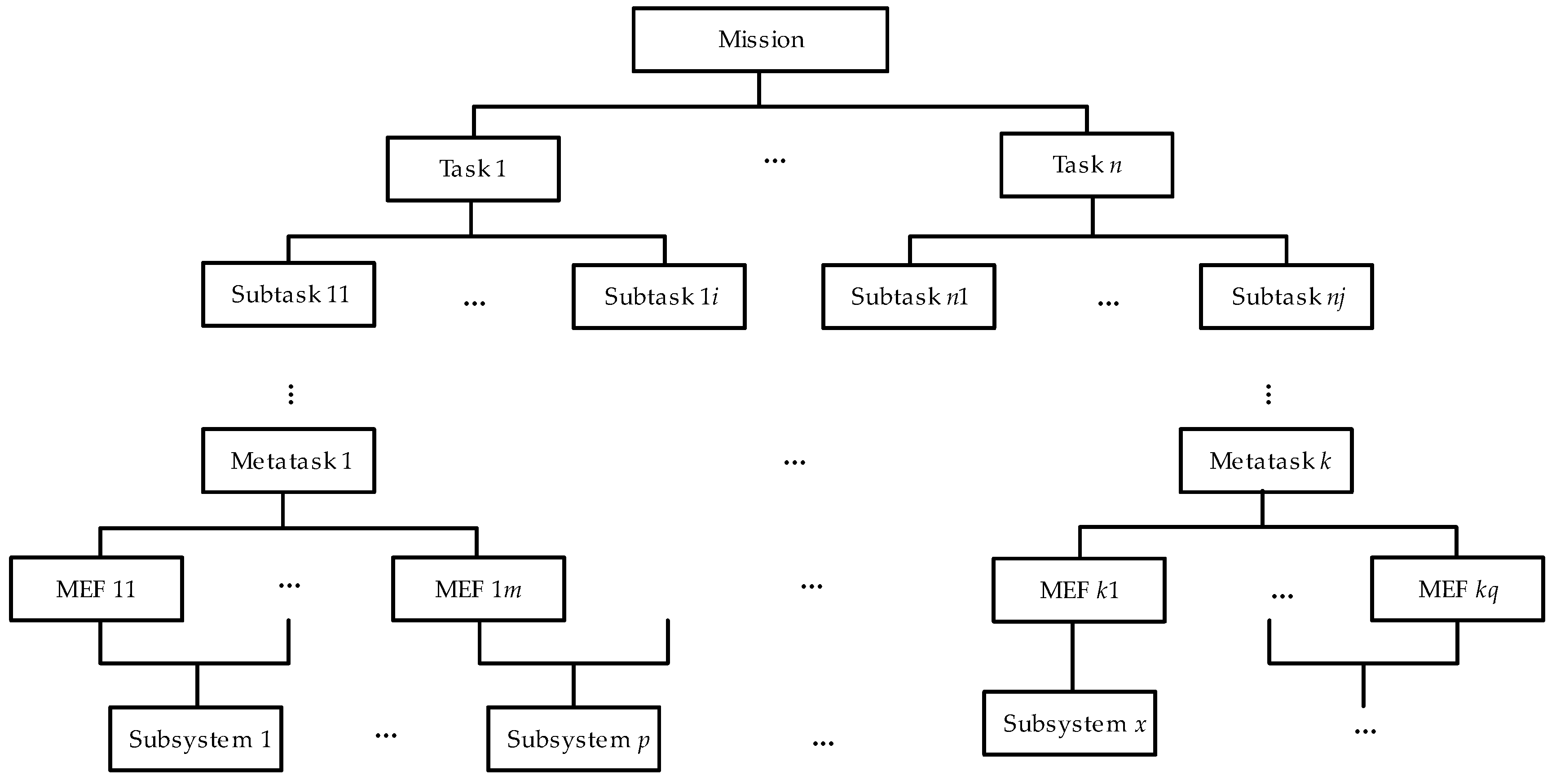
Figure 2.
BOM tree of two subsystems.
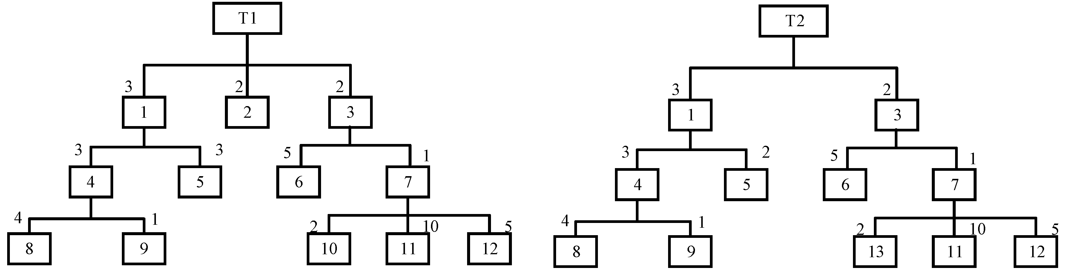
Figure 3.
PTs of two subsystems.
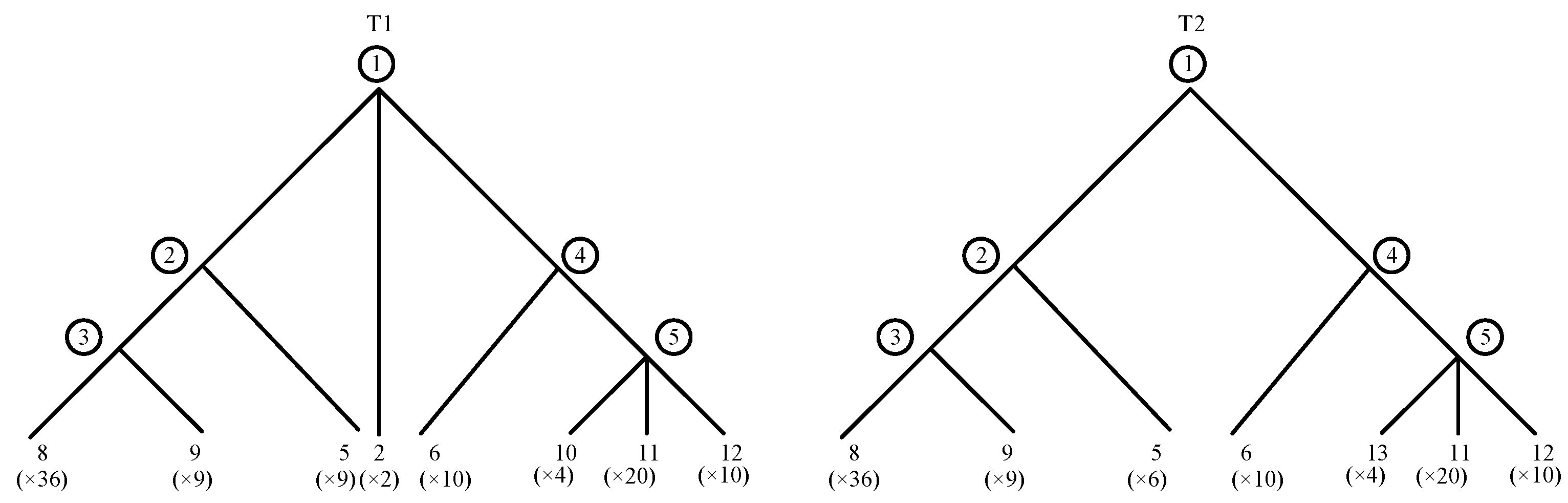
Figure 4.
PTs of two subsystems (taking the external circumstance into account).
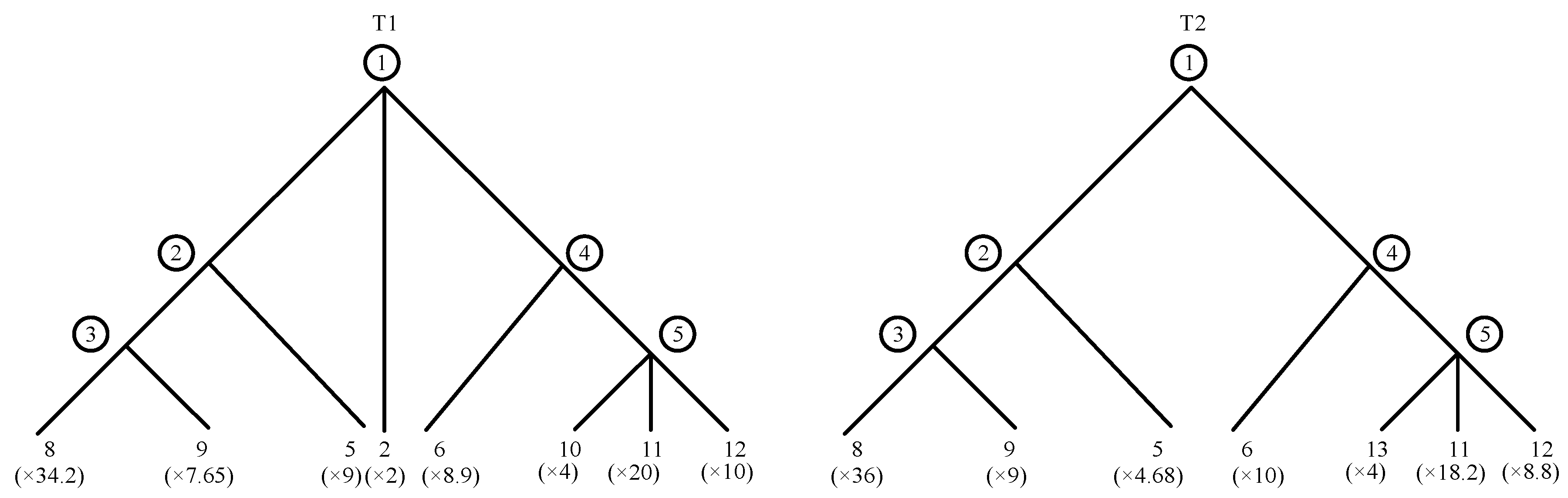
Figure 5.
Simplified tree structure for the mission of an equipment .
Figure 6.
BOM trees for the six hydraulic subsystems.
Figure 7.
PTs for the six hydraulic subsystems.
Figure 8.
Data for the six hydraulic subsystems.
Figure 9.
Posterior distributions of α1, β1, α2 and β2.
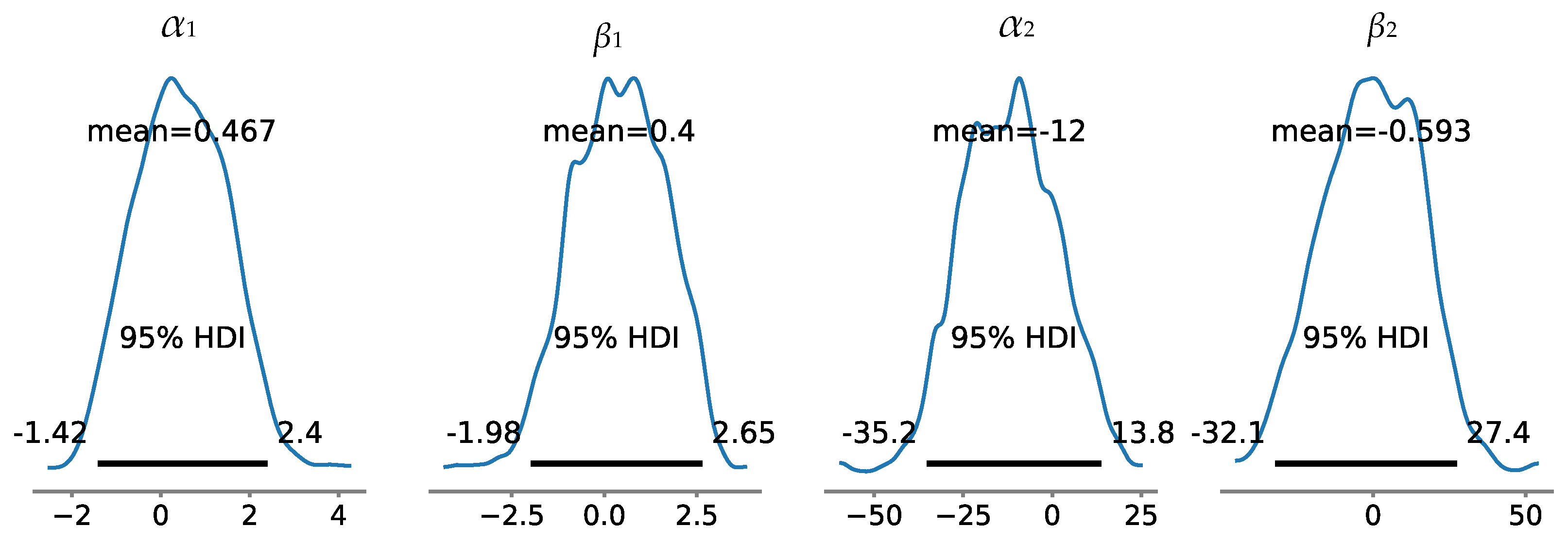
Figure 10.
Reliability distribution of the SSUT as a function of time.
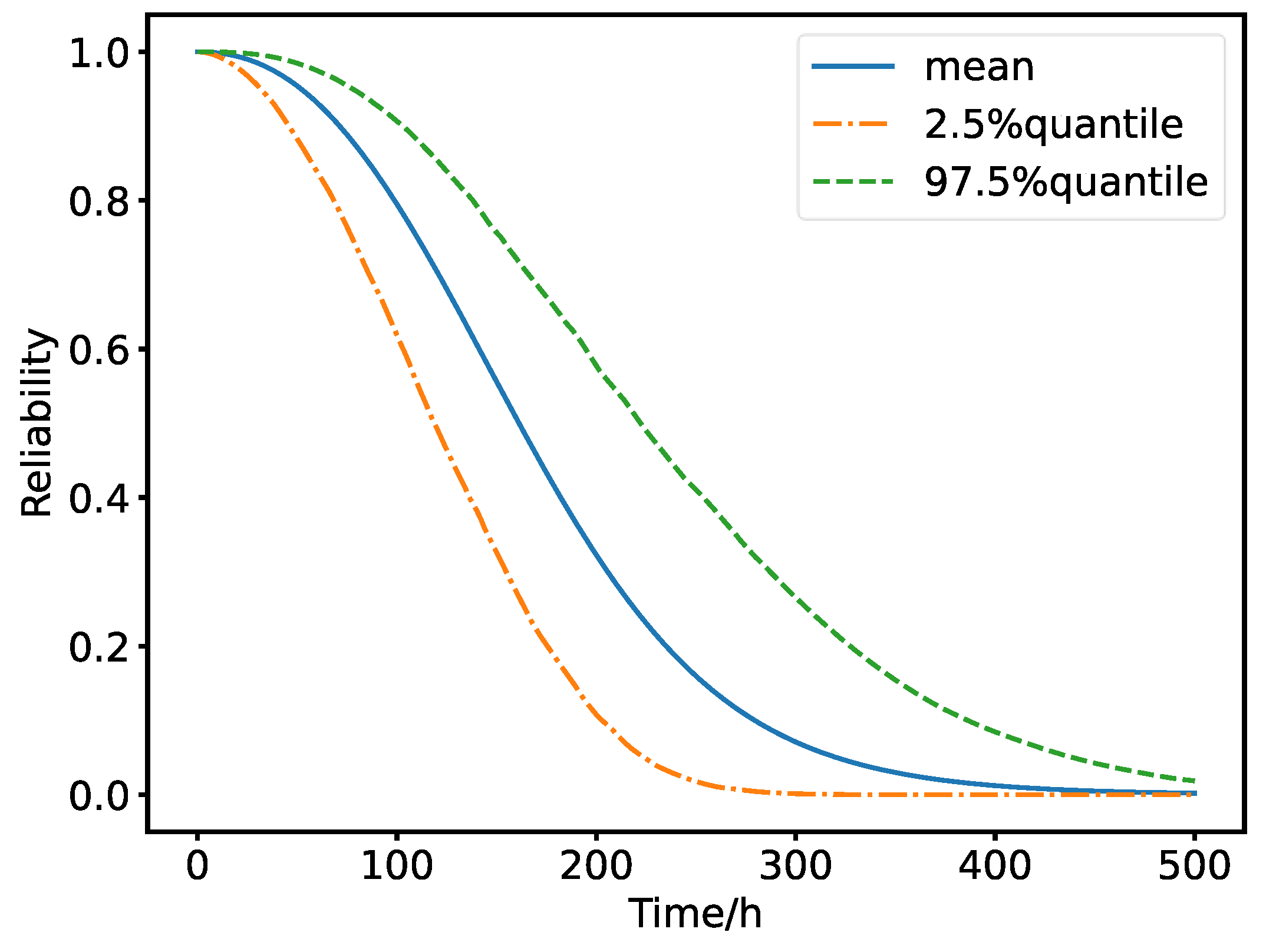

Table 1.
Summary of distances for mapping T1 nodes to T2 nodes.
| Node in T1 | Most similar node in T2 | Component in T1 but not in T2 | Shared component with higher quantity in T1 | Level difference | Quantity difference | Distance |
|---|---|---|---|---|---|---|
| 1 | 1 | 2,10 | 5 | 1,3,2 | 2,4,3 | 4.83 |
| 2 | 2 | - | 5 | 1 | 3 | 3 |
| 3 | 3 | - | - | - | - | 0 |
| 4 | 4 | 10 | - | 2 | 4 | 2 |
| 5 | 5 | 10 | - | 1 | 4 | 4 |
| Total | 13.83 | |||||
Table 2.
Summary of distances for mapping T2 nodes to T1 nodes.
| Node in T2 | Most similar node in T1 | Component in T2 but not in T1 | Shared component with higher quantity in T2 | Level difference | Quantity difference | Distance |
|---|---|---|---|---|---|---|
| 1 | 1 | 13 | - | 3 | 4 | 1.33 |
| 2 | 2 | - | - | - | - | 0 |
| 3 | 3 | - | - | - | - | 0 |
| 4 | 4 | 13 | - | 2 | 4 | 2 |
| 5 | 5 | 13 | - | 1 | 4 | 4 |
| Total | 7.33 | |||||
Table 3.
Basic components names and their assigned numbers.
| Name | Assigned number | Name | Assigned number |
|---|---|---|---|
| Pressure control valve | 1 | Copper pipe | 12 |
| Ceramic cartridge | 2 | Steel chrome-plated connector | 13 |
| Valve body | 3 | Housing partition manifold | 14 |
| Spring | 4 | Turret partition manifold | 15 |
| Direction control valve | 5 | Steel pipe | 16 |
| Cylinder block | 6 | Cooler | 17 |
| Guide sleeve | 7 | Copper pipe | 18 |
| Mandrel | 8 | Reinforced armor | 19 |
| Port plate | 9 | Copper alloy cartridge | 20 |
| Suction valve | 10 | Brass connector | 21 |
| Discharge valve | 11 |
Table 4.
Results from the simulation study.
| Subsystem | Parameter | Relative deviation | |
|---|---|---|---|
| Existing method | Proposed method | ||
| SSUT | m | 0.054 | -0.029 |
| λ | 0.178 | -0.027 | |
| Subsystem 1 | m | 0.315 | -0.035 |
| λ | 0162 | -0.074 | |
| Subsystem 2 | m | 0.263 | -0.076 |
| λ | 0.236 | -0.037 | |
Disclaimer/Publisher’s Note: The statements, opinions and data contained in all publications are solely those of the individual author(s) and contributor(s) and not of MDPI and/or the editor(s). MDPI and/or the editor(s) disclaim responsibility for any injury to people or property resulting from any ideas, methods, instructions or products referred to in the content. |
© 2025 by the authors. Licensee MDPI, Basel, Switzerland. This article is an open access article distributed under the terms and conditions of the Creative Commons Attribution (CC BY) license (http://creativecommons.org/licenses/by/4.0/).
Copyright: This open access article is published under a Creative Commons CC BY 4.0 license, which permit the free download, distribution, and reuse, provided that the author and preprint are cited in any reuse.


