
Submitted:
28 March 2025
Posted:
31 March 2025
You are already at the latest version
Abstract
Intelligence units are well known for their ability to gather critical data from unknown landscapes. Inspired by the capability of reconnaissance teams to zero in on the target location without any prior data, this paper proposes a novel hybrid metaheuristic optimisation algorithm, namely intelligence unit optimiser(IUO). The algorithm incorporates hill climbing and lévy search steps to explore the search space efficiently. A statistical comparison between the performance of the proposed algorithm and six other prominent algorithms has been done through 23 benchmark functions and five real-world engineering design optimisation problems. Test results show that IUO achieves faster convergence and provides competitive results in most of the cases.
Keywords:
metaheuristics
; optimisation
; nature-inspired
; swarm
; algorithm
; levy
; hill climb
; hybrid
1. Introduction
Traditional optimization methods, which typically rely on classical mathematical and probabilistic frameworks, often fall short in delivering effective solutions for complex real-world engineering challenges which possess intricate multimodal, high-dimensional, and nonconvex solution landscapes. In response, researchers have developed innovative solution strategies, termed meta-heuristic algorithms, designed to tackle challenging optimization problems with limited computational resources. These meta-heuristics have gained traction among scholars due to their numerous benefits over traditional optimisation approaches, which includes simplicity, non-reliance on differentiability, adaptability, and the ability to circumvent local optima. Some of the most popular metaheuristics are particle swarm optimisation[1], genetic algorithm[2], differential evolution[3], simulated annealing[4], tabu search[5], ant colony optimizer[6], bees algorithm[7] etc. Metaheuristic algorithms make trade-offs between exploration (global search) and exploitation (local search). Exploration behaviour allows the algorithm to move beyond local optimums and explore on a global scale, while local search focuses on smaller regions to find a refined solution. Almost all of the metaheuristic optimisation algorithms are stochastic in nature and they do not guarantee a similar solution on every run. They may converge at a near optimal solution or may even get stuck in a non optimal local optima. The performance of a metaheuristic optimisation algorithm is quantified by various measures like computational speed, rate of convergence, solution quality, time to find target solution level, consistency, solution diversity, etc[8]. The ’No free lunch theorem’ formulated by David Wolpert and William G. Macready[9] states that "any two optimisation algorithms are equivalent when their performance is averaged across all possible problems". This motivates researchers to develop new algorithms which work well in specific problem landscapes. More than 550[10] metaheuristic optimisation algorithms have been published till date and the annual publication rate is still increasing at a rapid pace.
2. Inspiration
Intelligence units have long stood at the forefront of strategic operations, serving as the nerve centers for gathering, analyzing, and disseminating critical information under conditions of uncertainty and high risk. These units are composed of highly trained operatives or agents or ’spies’ who are experts in identifying and exploring potential target areas.
Intelligence units typically operate in a three step strategy: The entire operation starts with an initial data collection from surveillance assets like high altitude reconnaissance platforms. In this phase, available data about the target area is acquired and analysed to find regions of interest. Once points of interest are identified, specialised field agents are inserted to conduct close-range intelligence operations. These agents infiltrate the target location and collect the required data. Another set of agents are assigned with shadow operations to ensure the success of the operation. They carry out stochastic surveillance, counter-intelligence and evasion operations. This tripartite structure -broad initial data collection, intensive targeted analysis, and agile adaptive response -embodies a balance between extensive exploration and focused exploitation. This approach of intelligence units has been adapted to solve optimisation problems as shown in Figure 1 and Figure 2.
The algorithm proceeds in three phases:
- Aerial Reconnaissance: A subset of spies perform a local search to find multiple local optima. These are then clustered to identify unique regions.
- Release of Agents: For each unique local optimum, a dedicated local search is applied to refine (exploit) that region.
- Levy Flight Search: The remaining spies perform a Levy flight move. If a Levy flight finds a promising candidate, spies are shifted to that region.
3. Hill Climbing Search
Greedy local search or hill climbing is a local search strategy in which the direction of search is along a direction that improves the fitness value. When a local move cannot improve the fitness value further, hill climb terminates. It is a nonbacktracking heuristic technique in which only the current state is stored, thereby minimising memory requirements[11]. Multiple variants of hill climbing exist, which includes simple hill climbing, steepest-ascent hill climbing, random-restart(stochastic) hill climbing, hill climbing[12], adaptive hill climbing[13] and late acceptance hill climbing[14]. Hill climbing search has been used to improve the local search capabilities of algorithms by many researchers[15,16,17,18,19,20,21,22,23,24,25,26,27].
4. Levy Flight
Lévy flight is a type of random walk characterized by step lengths that follow a heavy-tailed probability distribution, often a power law. This means that while most steps are relatively short, there is a significant probability of very long steps occurring. Such behavior contrasts with traditional random walks, like Brownian motion, where step lengths are typically uniform and lead to normal diffusion. Lévy flights are more efficient than Brownian random walks in exploring unknown, large-scale search spaces. A key parameter, denoted as (), determines the tail heaviness. For , the distribution corresponds to a normal (Gaussian) distribution, leading to standard Brownian motion. For , the distribution has heavier tails, resulting in occasional long jumps characteristic of Lévy flights. Lévy flight random number generation involves[28]:
- Direction Selection: Uniformly distributed random direction generation.
- Step Generation: Lévy distribution-compliant step generation. The Mantegna algorithm is an efficient method for symmetric Lévy stable distributions, allowing both positive and negative steps.
Lévy flights enhance search efficiency in uncertain environments and are observed in the foraging patterns of albatrosses, fruit flies, and spider monkeys. Beyond biology, Lévy flights appear in various physical phenomena, including molecular diffusion, cooling behavior, and noise dynamics under suitable conditions[29]. Levy flight search is used in multiple metaheuristic optimisers like Cuckoo search algorithm[30], Monarch butterfly optimiser[31], Lévy flight distribution optimiser[32], Moth search algorithm[33], Flower Pollination algorithm[34], Flying Squirrel optimizer[35], Butterfly algorithm[36], etc... The ability of levy flight search to explore the search space efficiency and escape local optima has made it a popular choice among researchers trying to improve the performance of metaheuristic optimisation algorithms[37,38,39,40,41,42,43,44,45,46,47,48,49,50,51,52,53,54,55,56,57,58,59,60]. Figure 3 shows the levy flight movement in three dimensional space with varying levels of step count and value.
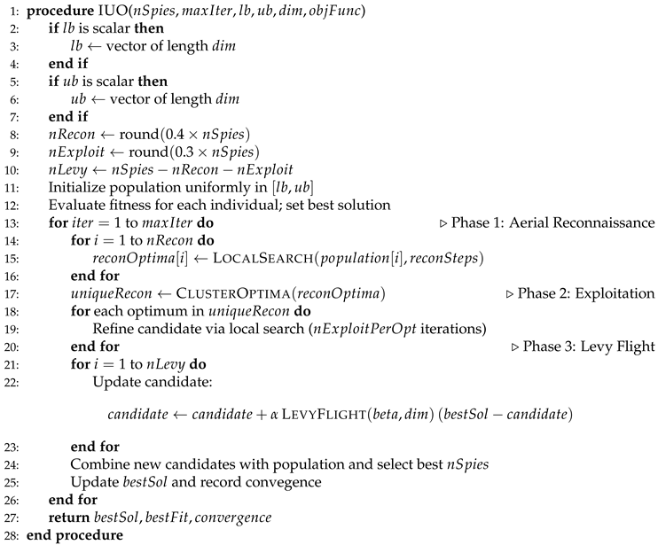
The pseudo code for the proposed algorithm is as follows:
| Algorithm 1 Pseudo code: IUO Algorithm |
 |
5. Testing
5.1. Benchmark Functions
The algorithm was tested on 23 benchmark functions out of which 6 are unimodal (F1, F2, F3, F4, F5, F6), 5 are multimodal (F7, F8, F9, F10, F11), 1 is fixed-dimension unimodal (F15), 8 are fixed-dimension multimodal (F12, F13, F14, F16, F17, F18, F19, F20) and 3 are composite (F21, F22, F23) functions. The proposed algorithm was compared with six popular optimisers namely simulated annealing[4], harmony search[61], particle swarm optimisation[1], bees algorithm[7], differential evolution[3] and grey wolf optimiser[62]. The population size for each algorithm was set at 50. Each algorithm was run for 200 iterations per test problem. A total of 30 runs were performed on each benchmark function, and statistical results were calculated. All the tests were run on Matlab R2024a in a stock HP laptop 15s-fr5xxx with 12th Gen Intel(R) Core(TM) i3-1215U, 1200 Mhz base clock speed, 6 cores and 8 logical processors with 8.00 GB installed RAM. Details about the twenty three benchmark functions is given in table below:
| Benchmark Functions (F1–F23) | |||||
| Func | Name | Equation | Dim | Bounds | |
| F1 | Sphere | 30 | 0 | ||
| F2 | Schwefel 2.22 | 10 | 0 | ||
| F3 | Schwefel 1.2 | 10 | 0 | ||
| F4 | Max-Abs | 10 | 0 | ||
| F5 | Rosenbrock | 10 | 0 | ||
| F6 | Shifted Sphere | 10 | 0 | ||
| F7 | Quartic with Noise | 10 | 0 (deterministic part) | ||
| F8 | Schwefel | 10 | |||
| F9 | Rastrigin | 10 | 0 | ||
| F10 | Ackley | 10 | 0 | ||
| F11 | Griewank | 10 | 0 | ||
| F12 | Hybrid 1 | 10 | 0 | ||
| F13 | Hybrid 2 | 10 | 0 | ||
| F14 | Function 14 | 2 | |||
| F15 | Function 15 | 4 | 0 | ||
| F16 | Six-Hump Camel | 2 | |||
| F17 | Branin Modified | 2 | and | ||
| F18 | Kowalik | 2 | 0 | ||
| F19 | Hartman 3 (modified) | 3 | |||
| F20 | Expanded Griewank-Rosenbrock | 6 | |||
| F21 | Composition 1 | , : [4,4,4,4], [1,1,1,1], [8,8,8,8], [6,6,6,6], [3,7,3,7] | 4 | ||
| F22 | Composition 2 | , (rows 1–7): | 4 | ||
| F23 | Composition 3 | , (rows 1–10): | 4 | ||
Note: The penalty function in F12 and F13 is defined as
Figure 4 and Figure 5 show the two dimensional version of the parameter spaces of the benchmark functions and the corresponding convergence curves for the compared algorithms. For multidimensional benchmark functions, except the first two dimensions, other values were fixed at the mid range for plotting.
5.2. Engineering Problems
The algorithm was also tested on five classical engineering problems namely ’Pressure vessel design problem’, ’Welded beam design problem’, ’Three bar truss design problem’, ’Gear train design problem’, and ’Spring design problem’.
5.2.1. Pressure Vessel Design Problem
This problem focuses on designing a cylindrical pressure vessel (with hemispherical heads) to minimize its total fabrication cost. The cost is modeled by a function that combines material, forming, and welding expenses. The objective function is typically expressed as
where and denote the shell and head thicknesses, R represents the inner radius, and L is the length of the cylindrical section. The design is subject to constraints that ensure safety and performance; for example, a minimum thickness constraint is
a similar constraint applies to , a volume constraint ensures that the vessel can contain a prescribed capacity
and an upper bound on the vessel’s length is
The decision variables are continuous with typical bounds such as
5.2.2. Welded Beam Design Problem
The welded beam design problem aims to design a beam with a welded joint that minimizes the overall fabrication cost while ensuring that the beam is strong enough to withstand the applied loads and meet serviceability requirements. A representative objective function is
where the design variables (weld thickness, beam length, width, and height) are selected to minimize cost. The design is constrained by limits on shear stress, bending stress, deflection, and geometric relationships (for example, ensuring one dimension does not exceed another). Typical variable bounds are be given by
ensuring that the dimensions remain practical for manufacturing.
5.2.3. Three Bar Truss Design Problem
The three-bar truss design problem is a classic structural optimization task where the goal is to minimize the weight (or cost) of a truss structure by selecting the optimal cross-sectional areas for its members. Its objective function is often defined as
which reflects the material cost or weight. In addition to minimizing weight, the design must satisfy constraints related to stress limits, deflection, and buckling to ensure the structure’s performance under load. Typically, the design variables and are continuous and are restricted within the range
5.2.4. Gear Train Design Problem
The gear train design problem is focused on achieving a specific gear transmission ratio while minimizing the deviation from the desired ratio. The goal is to match the desired ratio, commonly given as , with the actual ratio produced by the gear train. The objective function is often formulated as
where A, B, C, and D represent the numbers of teeth on the four gears. The design is constrained by the fact that these numbers must be integers and by practical manufacturing limits; typically, each variable is bounded by
5.2.5. Spring Design Problem
In the tension/compression spring design problem, the objective is to minimize the weight of the spring while ensuring that it meets performance criteria such as adequate stiffness, controlled deflection, and acceptable stress levels. A common objective function is expressed as
where d is the wire diameter, D is the mean coil diameter, and N is the number of active coils. The design is subject to constraints related to surge frequency, minimum deflection, and shear stress, which guarantee that the spring will function reliably under load. Typical variable bounds for the design variables are
Figure 10 and Table 6 show the convergence curves and statistical analysis results for the spring design problem.
6. Results and Discussion
From the results presented in appendix A1, it can be seen that the proposed algorithm achieves competitive results consistently in most of the cases. Convergence curves (4, 5) show that IUO starts converging faster than that of all the tested algorithms in most of the benchmark functions. It is to be noted that IUO outperforms other algorithms in four out of the five tested engineering design/optimisation problems indicating it’s potential to be used in real world applications. The algorithm’s simplicity and scalability make it an attractive option for complex optimisation applications.
7. Conclusion
Inspired by the ability of reconnaissance units to collect data about a target from unknown landscapes, a novel metaheuristic optimisation algorithm namely Intelligence unit optimiser (IUO) has been proposed. The algorithm operates in three main steps: Aerial reconnaissance (high exploration), local search (hill climbing search), and random search (levy search). An extensive statistical comparison has been made with six other well known optimisation algorithms on twenty three benchmark functions. The proposed algorithm has also been tested on five real world engineering problems namely ’pressure vessel design problem’, ’welded beam design problem’, ’three bar truss design problem’, ’gear train design problem’, and ’spring design problem’. The algorithm exhibits a faster convergence rate and provides competitive results in most of the cases, signalling it’s ability to be used for complex optimisation tasks. In future works, the proposed algorithm may be extended to solve multiobjective problems. Binary and mixed integer variants can also be introduced to deal with complex combinatorial problems.
Funding
This research did not receive any specific grant from funding agencies in the public, commercial, or not-for-profit sectors.
Appendix A Test Results

Table A1.
Statistical results for the tested functions and algorithms.
| Function | Algorithm | Mean | Std | Min | Max |
| F1 | |||||
| SA | 62433.43673 | 7768.95146 | 45239.38563 | 75883.81923 | |
| HS | 1249.2866 | 273.1516638 | 743.7009319 | 1915.892666 | |
| PSO | 0.001057276 | 0.004047286 | 1.10E-05 | 0.022295789 | |
| BA | 25017.21707 | 3504.097872 | 18631.21976 | 31274.01435 | |
| GWO | 3.37E-11 | 2.26E-11 | 2.96E-12 | 8.33E-11 | |
| DE | 37.5441381 | 8.61028452 | 24.94946723 | 60.66984996 | |
| IUO | 32.37804553 | 10.61614141 | 13.4573172 | 51.00279623 | |
| F2 | |||||
| SA | 18.36295351 | 6.672267579 | 7.076931221 | 32.96448013 | |
| HS | 0.079471092 | 0.023594179 | 0.044032883 | 0.149811012 | |
| PSO | 3.55E-11 | 1.54E-10 | 4.14E-13 | 8.49E-10 | |
| BA | 0.090063083 | 0.344210526 | 3.96E-06 | 1.472812127 | |
| GWO | 9.83E-16 | 1.14E-15 | 2.01E-17 | 5.09E-15 | |
| DE | 0.000255888 | 7.38E-05 | 0.000130674 | 0.000443308 | |
| IUO | 0.003145792 | 0.001053803 | 0.001442418 | 0.006450778 | |
| F3 | |||||
| SA | 11948.50796 | 4072.981039 | 4340.832821 | 21177.25268 | |
| HS | 310.1325075 | 251.8033197 | 31.43410841 | 1018.590352 | |
| PSO | 6.40E-07 | 2.30E-06 | 2.08E-09 | 1.26E-05 | |
| BA | 137.109036 | 134.1342083 | 2.286210625 | 527.2235794 | |
| GWO | 4.25E-11 | 8.71E-11 | 1.67E-16 | 3.84E-10 | |
| DE | 616.1802802 | 230.5128907 | 256.6827258 | 1281.595574 | |
| IUO | 1.841192485 | 1.230183378 | 0.265818736 | 4.604105555 | |
| F4 | |||||
| SA | 61.90222939 | 5.970313108 | 46.68933795 | 73.07573066 | |
| HS | 3.13531142 | 1.613334174 | 0.607581971 | 6.10649726 | |
| PSO | 8.66E-07 | 7.70E-07 | 4.27E-08 | 3.59E-06 | |
| BA | 6.821180961 | 3.415062859 | 8.75E-05 | 12.12018893 | |
| GWO | 8.27E-09 | 9.32E-09 | 1.09E-09 | 4.13E-08 | |
| DE | 1.176071114 | 0.260088314 | 0.721161425 | 1.807953871 | |
| IUO | 0.395980722 | 0.203113929 | 0.082361253 | 0.796531756 | |
| F5 | |||||
| SA | 11878427.6 | 8111771.84 | 1177427.947 | 29459907.58 | |
| HS | 175.8011595 | 369.9307086 | 8.120498914 | 1684.159273 | |
| PSO | 6.066544633 | 12.06508532 | 0.086844092 | 69.27417582 | |
| BA | 20.30444868 | 37.41255371 | 0.262753502 | 136.6166631 | |
| GWO | 9.689180766 | 15.65224652 | 6.131273917 | 92.49771537 | |
| DE | 31.22683651 | 9.3513016 | 15.96731436 | 54.87079562 | |
| IUO | 18.37273676 | 30.16940256 | 3.75274621 | 120.3541651 | |
| F6 | |||||
| SA | 11947.16695 | 3218.709875 | 3227.932093 | 17074.03432 | |
| HS | 0.233705708 | 0.166986815 | 0.062076282 | 0.862916745 | |
| PSO | 4.81E-21 | 9.14E-21 | 4.19E-23 | 4.38E-20 | |
| BA | 7.22E-10 | 3.55E-10 | 2.34E-10 | 1.74E-09 | |
| GWO | 1.68E-05 | 6.75E-06 | 7.11E-06 | 3.76E-05 | |
| DE | 1.09E-05 | 5.08E-06 | 4.02E-06 | 2.04E-05 | |
| IUO | 0.001233588 | 0.001038745 | 0.000188432 | 0.004789031 | |
| F7 | |||||
| SA | 0.51438883 | 0.260182354 | 0.09258187 | 0.968772181 | |
| HS | 0.024088447 | 0.011064288 | 0.007426729 | 0.051736731 | |
| PSO | 0.003327482 | 0.002023699 | 0.000935414 | 0.008710338 | |
| BA | 0.123380113 | 0.046343713 | 0.04916291 | 0.214171618 | |
| GWO | 0.001043936 | 0.000691388 | 0.000247504 | 0.003387708 | |
| DE | 0.014368542 | 0.005549152 | 0.00617549 | 0.031397965 | |
| IUO | 0.008833532 | 0.003763476 | 0.002908119 | 0.020820047 | |
| F8 | |||||
| SA | -1563.144539 | 314.6518183 | -2567.384431 | -1077.384132 | |
| HS | -4189.179383 | 0.44104534 | -4189.636528 | -4187.542989 | |
| PSO | -2561.141675 | 264.7997753 | -3005.426482 | -2117.059582 | |
| BA | -3593.656024 | 178.2608633 | -3972.673385 | -3202.832936 | |
| GWO | -2618.444952 | 257.3726529 | -3118.915189 | -2063.940216 | |
| DE | -4189.484811 | 0.333739905 | -4189.820261 | -4188.362586 | |
| IUO | -3472.442361 | 250.8292833 | -4189.803806 | -3102.610011 | |
| F9 | |||||
| SA | 39.02815186 | 13.8503912 | 16.94061421 | 73.09763413 | |
| HS | 2.384610868 | 1.217092504 | 0.143755009 | 4.250584513 | |
| PSO | 11.4420184 | 5.010678775 | 2.984877171 | 23.87899218 | |
| BA | 25.59017796 | 4.78166168 | 15.9193096 | 40.79315464 | |
| GWO | 2.138975871 | 2.810924111 | 0 | 11.17665732 | |
| DE | 5.489450764 | 1.585645318 | 2.89675587 | 8.844120071 | |
| IUO | 17.22654888 | 6.091772341 | 5.971123816 | 32.83649354 | |
| F10 | |||||
| SA | 18.94238928 | 0.768712335 | 17.20453552 | 19.915985 | |
| HS | 0.269984949 | 0.10582096 | 0.124355154 | 0.552963617 | |
| PSO | 2.38E-11 | 3.45E-11 | 6.61E-13 | 1.55E-10 | |
| BA | 2.502206384 | 2.989593641 | 5.88E-06 | 10.2849616 | |
| GWO | 9.72E-14 | 4.46E-14 | 4.31E-14 | 2.28E-13 | |
| DE | 0.001697522 | 0.000580729 | 0.000865156 | 0.003030376 | |
| IUO | 0.011793145 | 0.004907598 | 0.003948669 | 0.020203511 | |
| F11 | |||||
| SA | 120.560701 | 26.99154037 | 68.73662181 | 185.6755665 | |
| HS | 0.443671301 | 0.169024086 | 0.208449937 | 0.85209416 | |
| PSO | 0.091972371 | 0.044460805 | 0.019719489 | 0.201613939 | |
| BA | 0.07881936 | 0.155471747 | 6.63E-09 | 0.82416099 | |
| GWO | 0.064156395 | 0.085428481 | 0 | 0.394317387 | |
| DE | 0.130533317 | 0.046508441 | 0.03531855 | 0.225204327 | |
| IUO | 0.205312086 | 0.244867642 | 0.017103136 | 0.903152178 | |
| F12 | |||||
| SA | 40009327.02 | 23546617.51 | 3567106.055 | 99703911.67 | |
| HS | 0.083299246 | 0.14298004 | 0.000730185 | 0.488961732 | |
| PSO | 2.84E-21 | 1.53E-20 | 2.71E-25 | 8.37E-20 | |
| BA | 1.905663163 | 1.607971293 | 7.47E-12 | 5.889452381 | |
| GWO | 0.002023484 | 0.006155006 | 1.25E-06 | 0.02021771 | |
| DE | 4.73E-07 | 3.06E-07 | 1.59E-07 | 1.44E-06 | |
| IUO | 0.01038726 | 0.056780491 | 2.49E-06 | 0.311020148 | |
| F13 | |||||
| SA | 77256912.71 | 47032401.41 | 4932817.351 | 222856443.1 | |
| HS | 0.024392041 | 0.012884649 | 0.004324166 | 0.051253222 | |
| PSO | 0.000366246 | 0.002006009 | 2.69E-24 | 0.010987366 | |
| BA | 0.715347513 | 1.819931522 | 1.04E-11 | 9.075838629 | |
| GWO | 0.006539435 | 0.024799544 | 1.03E-05 | 0.097776445 | |
| DE | 1.94E-06 | 9.57E-07 | 9.27E-07 | 5.13E-06 | |
| IUO | 0.001878609 | 0.004149939 | 5.83E-06 | 0.011016885 | |
| F14 | |||||
| SA | 11.83216802 | 6.233484373 | 0.998003839 | 23.80943463 | |
| HS | 0.998003838 | 9.51E-10 | 0.998003838 | 0.998003842 | |
| PSO | 2.246555945 | 2.243066709 | 0.998003838 | 10.76318067 | |
| BA | 0.998141166 | 0.000752158 | 0.998003838 | 1.002123583 | |
| GWO | 4.492820343 | 4.075456867 | 0.998003838 | 12.67050581 | |
| DE | 0.998003838 | 4.12E-17 | 0.998003838 | 0.998003838 | |
| IUO | 0.998003838 | 2.16E-16 | 0.998003838 | 0.998003838 | |
| F15 | |||||
| SA | 0.027365887 | 0.021287903 | 0.001284138 | 0.080117468 | |
| HS | 0.004048867 | 0.006600727 | 0.000741744 | 0.020549943 | |
| PSO | 0.000636633 | 0.000474129 | 0.000307486 | 0.001594435 | |
| BA | 0.000435519 | 0.000103931 | 0.000307517 | 0.000715046 | |
| GWO | 0.005865168 | 0.00889525 | 0.00031033 | 0.02036338 | |
| DE | 0.000828791 | 0.000146989 | 0.000442421 | 0.001302292 | |
| IUO | 0.000585381 | 0.000197889 | 0.000313647 | 0.001247569 | |
| F16 | |||||
| SA | -1.020411482 | 0.024475726 | -1.031379534 | -0.914785836 | |
| HS | -1.03162378 | 6.07E-06 | -1.03162835 | -1.031599982 | |
| PSO | -1.031628453 | 6.32E-16 | -1.031628453 | -1.031628453 | |
| BA | -1.031628453 | 5.43E-15 | -1.031628453 | -1.031628453 | |
| GWO | -1.031628375 | 8.17E-08 | -1.03162845 | -1.031628164 | |
| DE | -1.031628453 | 6.05E-16 | -1.031628453 | -1.031628453 | |
| IUO | -1.031628453 | 4.79E-16 | -1.031628453 | -1.031628453 | |
| F17 | |||||
| SA | 0.405076124 | 0.008924657 | 0.398189894 | 0.443853141 | |
| HS | 0.397897074 | 1.45E-05 | 0.397887375 | 0.397956158 | |
| PSO | 0.397887358 | 0 | 0.397887358 | 0.397887358 | |
| BA | 0.397887358 | 6.84E-15 | 0.397887358 | 0.397887358 | |
| GWO | 0.397896815 | 1.18E-05 | 0.397887821 | 0.397946289 | |
| DE | 0.397887358 | 2.69E-13 | 0.397887358 | 0.397887358 | |
| IUO | 0.397887358 | 0 | 0.397887358 | 0.397887358 | |
| F18 | |||||
| SA | 12.77408968 | 20.83097224 | 3.001505739 | 83.62962391 | |
| HS | 8.581796149 | 11.39151745 | 3.000000681 | 35.43761728 | |
| PSO | 3 | 2.19E-15 | 3 | 3 | |
| BA | 3 | 6.19E-14 | 3 | 3 | |
| GWO | 3.000097543 | 0.0001322 | 3.000000024 | 3.000430126 | |
| DE | 3 | 1.45E-15 | 3 | 3 | |
| IUO | 3 | 4.49E-15 | 3 | 3 | |
| F19 | |||||
| SA | -0.220588372 | 0.10116896 | -0.300478907 | -0.000347605 | |
| HS | -0.300478907 | 2.26E-16 | -0.300478907 | -0.300478907 | |
| PSO | -0.300478907 | 2.26E-16 | -0.300478907 | -0.300478907 | |
| BA | -3.862782148 | 5.14E-15 | -3.862782148 | -3.862782148 | |
| GWO | -0.300478907 | 2.26E-16 | -0.300478907 | -0.300478907 | |
| DE | -0.300478907 | 2.26E-16 | -0.300478907 | -0.300478907 | |
| IUO | -0.300478907 | 2.26E-16 | -0.300478907 | -0.300478907 | |
| F20 | |||||
| SA | -2.695955761 | 0.414559588 | -3.285683801 | -1.702189319 | |
| HS | -3.294248287 | 0.051146885 | -3.321994949 | -3.203084582 | |
| PSO | -3.290290339 | 0.053475325 | -3.321995172 | -3.20310205 | |
| BA | -3.321995172 | 1.33E-14 | -3.321995172 | -3.321995172 | |
| GWO | -3.24346263 | 0.073909566 | -3.321972986 | -3.083840374 | |
| DE | -3.321873929 | 0.000288818 | -3.321995172 | -3.320798714 | |
| IUO | -3.321995166 | 4.83E-09 | -3.321995171 | -3.321995153 | |
| F21 | |||||
| SA | -1.714619162 | 2.024260006 | -9.897187976 | -0.391506724 | |
| HS | -5.189233591 | 3.573722653 | -10.15300012 | -2.630405634 | |
| PSO | -6.222113764 | 3.393421646 | -10.15319968 | -2.630471668 | |
| BA | -10.15319968 | 2.43E-12 | -10.15319968 | -10.15319968 | |
| GWO | -8.645932852 | 2.826376144 | -10.15219898 | -2.680683312 | |
| DE | -9.999818057 | 0.308363667 | -10.15319476 | -8.720708792 | |
| IUO | -10.15319968 | 7.64E-10 | -10.15319968 | -10.15319968 | |
| F22 | |||||
| SA | -2.456897676 | 3.021228862 | -10.34766703 | -0.442580395 | |
| HS | -5.183809193 | 3.22803213 | -10.40289327 | -2.751880805 | |
| PSO | -6.627709627 | 3.656465615 | -10.40294057 | -2.751933564 | |
| BA | -10.40294057 | 9.70E-12 | -10.40294057 | -10.40294057 | |
| GWO | -10.21860033 | 0.961564834 | -10.40145825 | -5.127497884 | |
| DE | -10.27352691 | 0.259594122 | -10.40293792 | -9.105132677 | |
| IUO | -10.40294057 | 1.56E-09 | -10.40294057 | -10.40294056 | |
| F23 | |||||
| SA | -2.220822783 | 2.473606994 | -10.47918607 | -0.680063691 | |
| HS | -6.427662556 | 3.933530645 | -10.53637188 | -2.421681743 | |
| PSO | -7.651687855 | 3.663524603 | -10.53640982 | -2.421734027 | |
| BA | -10.53640982 | 4.15E-12 | -10.53640982 | -10.53640982 | |
| GWO | -10.52906651 | 0.004007121 | -10.53490156 | -10.51485343 | |
| DE | -10.47092219 | 0.096242344 | -10.53640982 | -10.23851441 | |
| IUO | -10.35771771 | 0.978736954 | -10.53640982 | -5.175646741 | |
References
- Kennedy, J.; Eberhart, R. Particle swarm optimization. In Proceedings of the Proceedings of ICNN’95-international conference on neural networks. ieee, 1995, Vol. 4, pp. 1942–1948.
- Michalewicz, Z. Genetic algorithms+ data structures= evolution programs; Springer Science & Business Media, 2013.
- Storn, R.; Price, K. Differential evolution–a simple and efficient heuristic for global optimization over continuous spaces. Journal of global optimization 1997, 11, 341–359. [Google Scholar] [CrossRef]
- Kirkpatrick, S.; Gelatt Jr, C.D.; Vecchi, M.P. Optimization by simulated annealing. science 1983, 220, 671–680. [Google Scholar] [CrossRef] [PubMed]
- Glover, F.; Laguna, M. Tabu search; Springer, 1998.
- Dorigo, M.; Birattari, M.; Stutzle, T. Ant colony optimization. IEEE computational intelligence magazine 2007, 1, 28–39. [Google Scholar] [CrossRef]
- Pham, D.T.; Ghanbarzadeh, A.; Koç, E.; Otri, S.; Rahim, S.; Zaidi, M. The bees algorithm—a novel tool for complex optimisation problems. In Intelligent production machines and systems; Elsevier, 2006; pp. 454–459.
- Halim, A.H.; Ismail, I.; Das, S. Performance assessment of the metaheuristic optimization algorithms: an exhaustive review. Artificial Intelligence Review 2021, 54, 2323–2409. [Google Scholar] [CrossRef]
- Wolpert, D.H.; Macready, W.G. No free lunch theorems for optimization. IEEE transactions on evolutionary computation 1997, 1, 67–82. [Google Scholar] [CrossRef]
- Ma, Z.; Wu, G.; Suganthan, P.N.; Song, A.; Luo, Q. Performance assessment and exhaustive listing of 500+ nature-inspired metaheuristic algorithms. Swarm and Evolutionary Computation 2023, 77, 101248. [Google Scholar] [CrossRef]
- Selman, B.; Gomes, C.P. Hill-climbing search. Encyclopedia of cognitive science 2006, 81, 10. [Google Scholar]
- Al-Betar, M.A. β-hill climbing: an exploratory local search. Neural Computing and Applications 2017, 28, 153–168. [Google Scholar] [CrossRef]
- Al-Betar, M.A.; Aljarah, I.; Awadallah, M.A.; Faris, H.; Mirjalili, S. Adaptive β-hill climbing for optimization. Soft Computing 2019, 23, 13489–13512. [Google Scholar] [CrossRef]
- Burke, E.K.; Bykov, Y. The late acceptance hill-climbing heuristic. European Journal of Operational Research 2017, 258, 70–78. [Google Scholar] [CrossRef]
- Dehkordi, A.A.; Etaati, B.; Neshat, M.; Mirjalili, S. Adaptive Chaotic Marine Predators Hill Climbing Algorithm for Large-Scale Design Optimizations. Ieee Access 2023, 11, 39269–39294. [Google Scholar] [CrossRef]
- Shehab, M.; Khader, A.T.; Al-Betar, M.A.; Abualigah, L.M. Hybridizing cuckoo search algorithm with hill climbing for numerical optimization problems. In Proceedings of the 2017 8th International conference on information technology (ICIT). IEEE, 2017, pp. 36–43.
- Emambocus, B.A.S.; Jasser, M.B.; Amphawan, A. An optimized continuous dragonfly algorithm using hill climbing local search to tackle the low exploitation problem. IEEE Access 2022, 10, 95030–95045. [Google Scholar] [CrossRef]
- Al-Qablan, T.A.; Noor, M.H.M.; Al-Betar, M.A.; Khader, A.T. Improved binary gray wolf optimizer based on adaptive β-hill climbing for feature selection. IEEE Access 2023, 11, 59866–59881. [Google Scholar] [CrossRef]
- Kumar, R.; Tyagi, S.; Sharma, M. Memetic algorithm: hybridization of hill climbing with selection operator. International J. Soft Computing and Engineering (IJSCE) ISSN 2013, pp. 2231–2307.
- Alyasseri, Z.A.A.; Al-Betar, M.A.; Awadallah, M.A.; Makhadmeh, S.N.; Abasi, A.K.; Doush, I.A.; Alomari, O.A. A hybrid flower pollination with β-hill climbing algorithm for global optimization. Journal of King Saud University-Computer and Information Sciences 2022, 34, 4821–4835. [Google Scholar] [CrossRef]
- Lim, A.; Lin, J.; Rodrigues, B.; Xiao, F. Ant colony optimization with hill climbing for the bandwidth minimization problem. Applied Soft Computing 2006, 6, 180–188. [Google Scholar] [CrossRef]
- Allouani, F.; Abboudi, A.; Gao, X.Z.; Bououden, S.; Boulkaibet, I.; Khezami, N.; Lajmi, F. A spider monkey optimization based on beta-hill climbing optimizer for unmanned combat aerial vehicle (UCAV). Applied Sciences 2023, 13, 3273. [Google Scholar] [CrossRef]
- Alanazi, M.; Alanazi, A.; Memon, Z.A.; Csaba, M.; Mosavi, A. Hill climbing artificial electric field algorithm for maximum power point tracking of photovoltaics. Frontiers in Energy Research 2022, 10, 905310. [Google Scholar] [CrossRef]
- Yuce, B.; Pham, D.; Packianather, M.S.; Mastrocinque, E. An enhancement to the Bees Algorithm with slope angle computation and Hill Climbing Algorithm and its applications on scheduling and continuous-type optimisation problem. Production & Manufacturing Research 2015, 3, 3–19. [Google Scholar] [CrossRef]
- Xiao, Y.; Sun, X.; Guo, Y.; Li, S.; Zhang, Y.; Wang, Y. An Improved Gorilla Troops Optimizer Based on Lens Opposition-Based Learning and Adaptive β-Hill Climbing for Global Optimization. Cmes-Computer Modeling In Engineering & Sciences 2022, 131. [Google Scholar] [CrossRef]
- Al-saedi, A.; Mawlood-Yunis, A.R. Binary Black Widow with Hill Climbing. In Proceedings of the Optimization and Learning: 6th International Conference, OLA 2023, Malaga, Spain, May 3–5, 2023, Proceedings. Springer Nature, 2023, p. 263.
- Chatterjee, B.; Bhattacharyya, T.; Ghosh, K.K.; Singh, P.K.; Geem, Z.W.; Sarkar, R. Late acceptance hill climbing based social ski driver algorithm for feature selection. IEEe Access 2020, 8, 75393–75408. [Google Scholar] [CrossRef]
- Li, J.; An, Q.; Lei, H.; Deng, Q.; Wang, G.G. Survey of lévy flight-based metaheuristics for optimization. Mathematics 2022, 10, 2785. [Google Scholar] [CrossRef]
- Yang, X.S.; Press, L. Nature-inspired metaheuristic algorithms second edition, 2010.
- Gandomi, A.H.; Yang, X.S.; Alavi, A.H. Cuckoo search algorithm: a metaheuristic approach to solve structural optimization problems. Engineering with computers 2013, 29, 17–35. [Google Scholar] [CrossRef]
- Wang, G.G.; Deb, S.; Cui, Z. Monarch butterfly optimization. Neural computing and applications 2019, 31, 1995–2014. [Google Scholar] [CrossRef]
- Houssein, E.H.; Saad, M.R.; Hashim, F.A.; Shaban, H.; Hassaballah, M. Lévy flight distribution: A new metaheuristic algorithm for solving engineering optimization problems. Engineering Applications of Artificial Intelligence 2020, 94, 103731. [Google Scholar] [CrossRef]
- Wang, G.G. Moth search algorithm: a bio-inspired metaheuristic algorithm for global optimization problems. Memetic Computing 2018, 10, 151–164. [Google Scholar] [CrossRef]
- Abdel-Basset, M.; Shawky, L.A. Flower pollination algorithm: a comprehensive review. Artificial Intelligence Review 2019, 52, 2533–2557. [Google Scholar] [CrossRef]
- Azizyan, G.; Miarnaeimi, F.; Rashki, M.; Shabakhty, N. Flying Squirrel Optimizer (FSO): A novel SI-based optimization algorithm for engineering problems. Iran. J. Optim 2019, 11, 177–205. [Google Scholar]
- Arora, S.; Singh, S. Butterfly algorithm with levy flights for global optimization. In Proceedings of the 2015 International conference on signal processing, computing and control (ISPCC). IEEE, 2015, pp. 220–224.
- Yang, X.S. Firefly algorithm, Levy flights and global optimization. In Proceedings of the Research and development in intelligent systems XXVI: Incorporating applications and innovations in intelligent systems XVII. Springer, 2010, pp. 209–218.
- Tang, D.; Yang, J.; Dong, S.; Liu, Z. A lévy flight-based shuffled frog-leaping algorithm and its applications for continuous optimization problems. Applied Soft Computing 2016, 49, 641–662. [Google Scholar] [CrossRef]
- Chegini, S.N.; Bagheri, A.; Najafi, F. PSOSCALF: A new hybrid PSO based on Sine Cosine Algorithm and Levy flight for solving optimization problems. Applied Soft Computing 2018, 73, 697–726. [Google Scholar] [CrossRef]
- Iacca, G.; dos Santos Junior, V.C.; de Melo, V.V. An improved Jaya optimization algorithm with Lévy flight. Expert Systems with Applications 2021, 165, 113902. [Google Scholar] [CrossRef]
- Kaidi, W.; Khishe, M.; Mohammadi, M. Dynamic levy flight chimp optimization. Knowledge-Based Systems 2022, 235, 107625. [Google Scholar] [CrossRef]
- Seyyedabbasi, A. WOASCALF: A new hybrid whale optimization algorithm based on sine cosine algorithm and levy flight to solve global optimization problems. Advances in Engineering Software 2022, 173, 103272. [Google Scholar] [CrossRef]
- Dinkar, S.K.; Deep, K. An efficient opposition based Lévy Flight Antlion optimizer for optimization problems. Journal of computational science 2018, 29, 119–141. [Google Scholar] [CrossRef]
- Ling, Y.; Zhou, Y.; Luo, Q. Lévy flight trajectory-based whale optimization algorithm for global optimization. IEEE access 2017, 5, 6168–6186. [Google Scholar] [CrossRef]
- Wang, G.; Guo, L.; Gandomi, A.H.; Cao, L.; Alavi, A.H.; Duan, H.; Li, J. Levy-flight krill herd algorithm. Mathematical Problems in Engineering 2013, 2013, 682073. [Google Scholar] [CrossRef]
- Wu, L.; Wu, J.; Wang, T. Enhancing grasshopper optimization algorithm (GOA) with levy flight for engineering applications. Scientific reports 2023, 13, 124. [Google Scholar] [CrossRef]
- Wang, W.c.; Xu, L.; Chau, K.w.; Liu, C.j.; Ma, Q.; Xu, D.m. Cε-LDE: A lightweight variant of differential evolution algorithm with combined ε constrained method and Lévy flight for constrained optimization problems. Expert Systems with Applications 2023, 211, 118644. [Google Scholar] [CrossRef]
- Haklı, H.; Uğuz, H. A novel particle swarm optimization algorithm with Levy flight. Applied Soft Computing 2014, 23, 333–345. [Google Scholar] [CrossRef]
- Liu, Y.; Cao, B. A novel ant colony optimization algorithm with Levy flight. Ieee Access 2020, 8, 67205–67213. [Google Scholar] [CrossRef]
- Sharma, H.; Bansal, J.C.; Arya, K.; Yang, X.S. Lévy flight artificial bee colony algorithm. International Journal of Systems Science 2016, 47, 2652–2670. [Google Scholar] [CrossRef]
- Lin, J.H.; Chou, C.W.; Yang, C.H.; Tsai, H.L.; et al. A chaotic Levy flight bat algorithm for parameter estimation in nonlinear dynamic biological systems. Computer and Information Technology 2012, 2, 56–63. [Google Scholar]
- Abdulwahab, H.A.; Noraziah, A.; Alsewari, A.A.; Salih, S.Q. An enhanced version of black hole algorithm via levy flight for optimization and data clustering problems. Ieee Access 2019, 7, 142085–142096. [Google Scholar] [CrossRef]
- Saravanan, G.; Neelakandan, S.; Ezhumalai, P.; Maurya, S. Improved wild horse optimization with levy flight algorithm for effective task scheduling in cloud computing. Journal of Cloud Computing 2023, 12, 24. [Google Scholar] [CrossRef]
- Zhang, J.; Wang, J.S. Improved salp swarm algorithm based on levy flight and sine cosine operator. Ieee Access 2020, 8, 99740–99771. [Google Scholar] [CrossRef]
- Chen, D.; Zhao, J.; Huang, P.; Deng, X.; Lu, T. An improved sparrow search algorithm based on levy flight and opposition-based learning. Assembly Automation 2021, 41, 697–713. [Google Scholar] [CrossRef]
- Ewees, A.A.; Mostafa, R.R.; Ghoniem, R.M.; Gaheen, M.A. Improved seagull optimization algorithm using Lévy flight and mutation operator for feature selection. Neural Computing and Applications 2022, 34, 7437–7472. [Google Scholar] [CrossRef]
- Boudjemaa, R.; Oliva, D.; Ouaar, F. Fractional Lévy flight bat algorithm for global optimisation. International Journal of Bio-Inspired Computation 2020, 15, 100–112. [Google Scholar] [CrossRef]
- Ekinci, S.; Izci, D.; Abu Zitar, R.; Alsoud, A.R.; Abualigah, L. Development of Lévy flight-based reptile search algorithm with local search ability for power systems engineering design problems. Neural Computing and Applications 2022, 34, 20263–20283. [Google Scholar] [CrossRef]
- Bhatt, B.; Sharma, H.; Arora, K.; Joshi, G.P.; Shrestha, B. Levy flight-based improved grey wolf optimization: a solution for various engineering problems. Mathematics 2023, 11, 1745. [Google Scholar] [CrossRef]
- Wang, W.; Tian, J. An improved nonlinear tuna swarm optimization algorithm based on circle chaos map and levy flight operator. Electronics 2022, 11, 3678. [Google Scholar] [CrossRef]
- Geem, Z.W.; Kim, J.H.; Loganathan, G.V. A new heuristic optimization algorithm: harmony search. simulation 2001, 76, 60–68. [Google Scholar] [CrossRef]
- Mirjalili, S.; Mirjalili, S.M.; Lewis, A. Grey wolf optimizer. Advances in engineering software 2014, 69, 46–61. [Google Scholar] [CrossRef]
Figure 1.
Inspiration of IUO algorithm
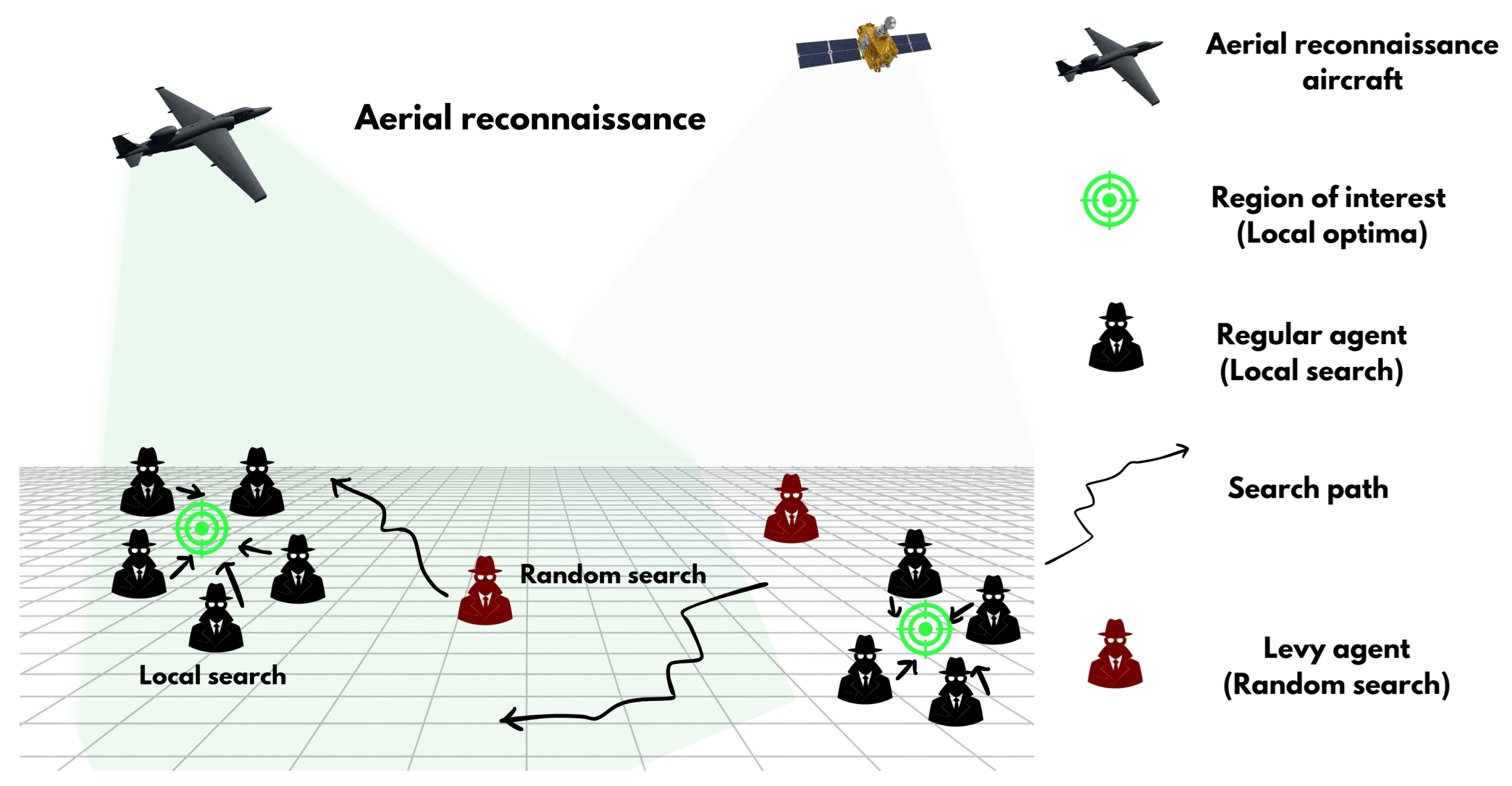
Figure 2.
Comparison of reconnaissance operation with IUO
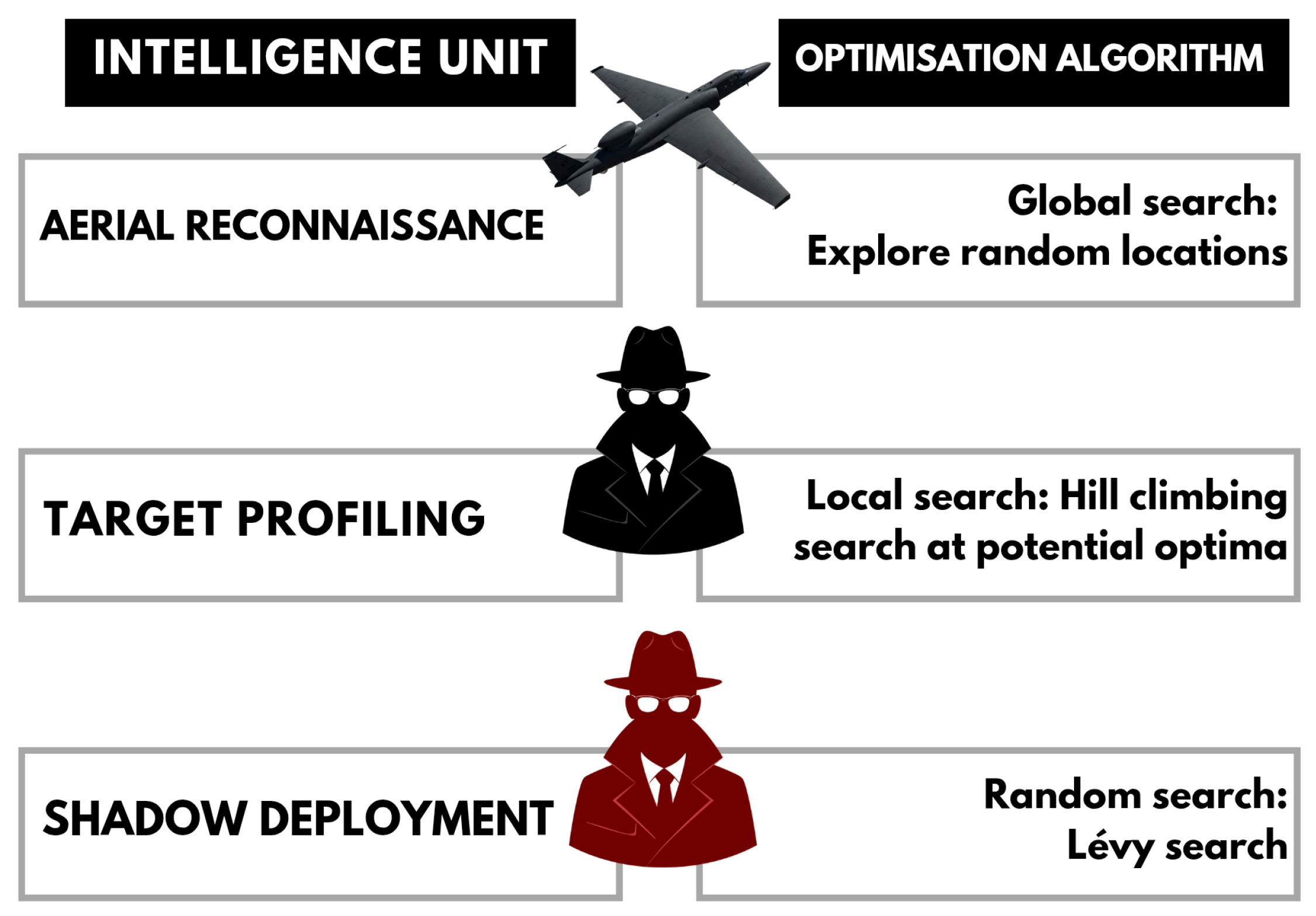
Figure 3.
Visualization of Levy flight in 3D at varying step count and values.
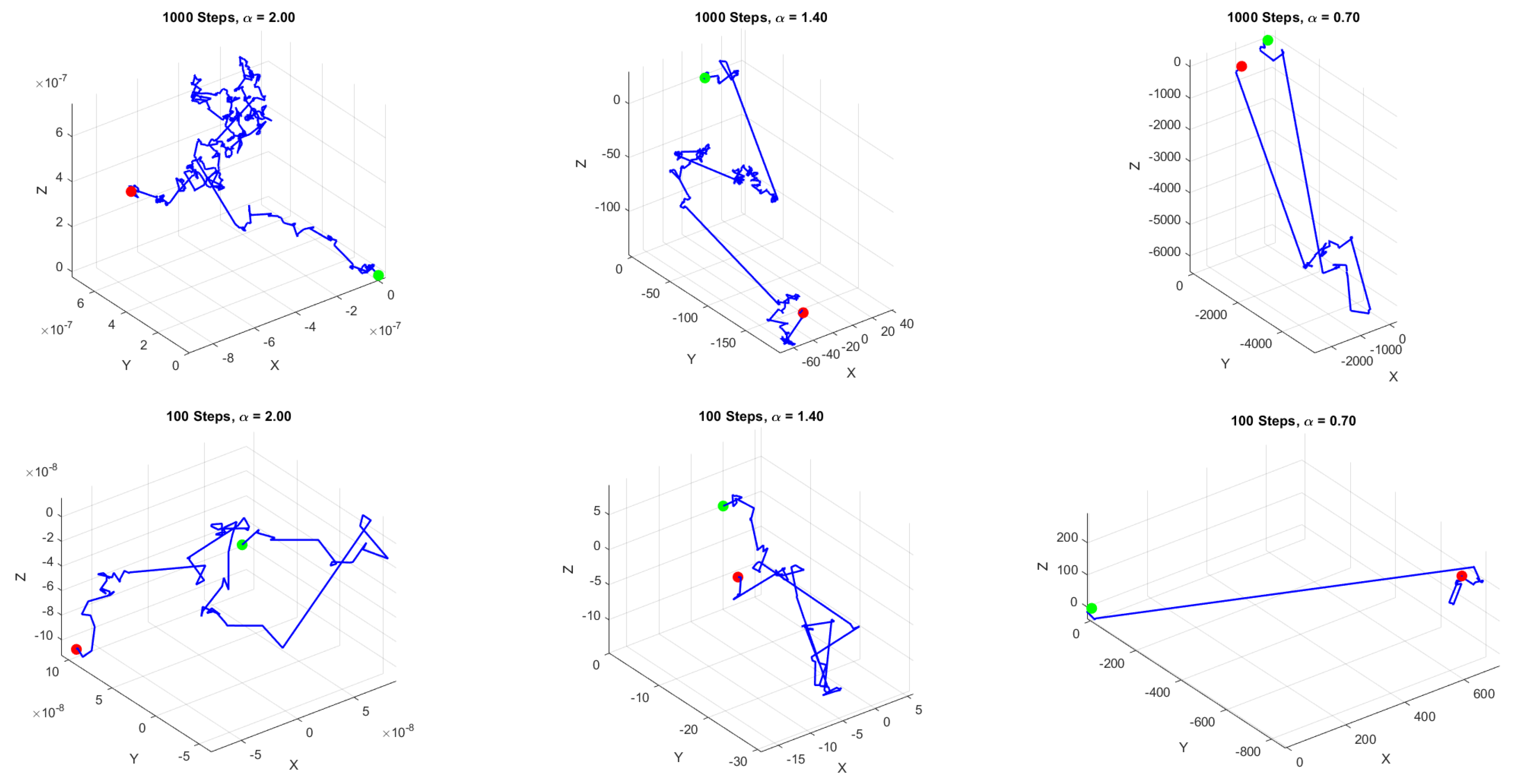
Figure 4.
Convergence curves (F1-F10)
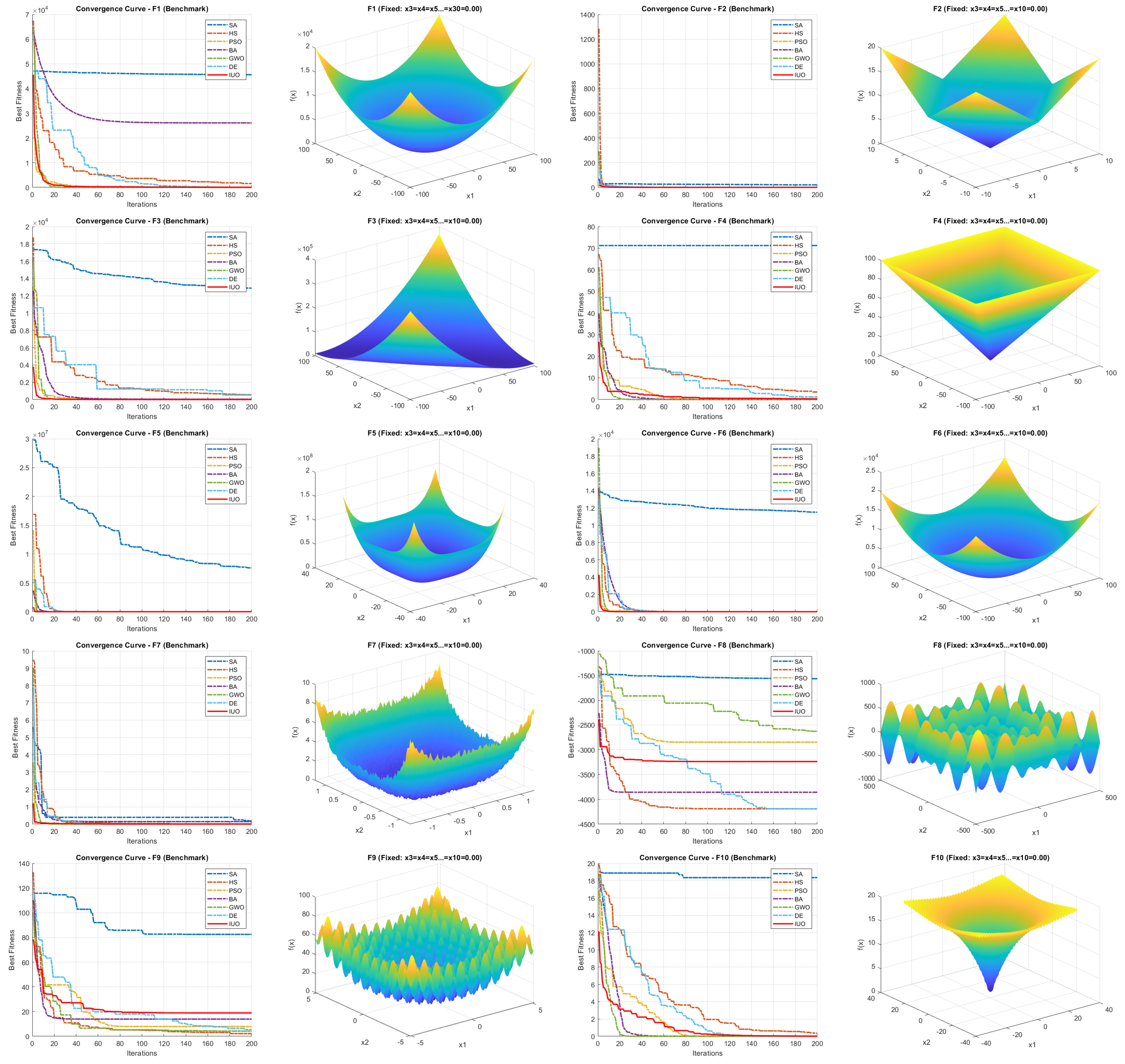
Figure 5.
Convergence curves (F11-F23)
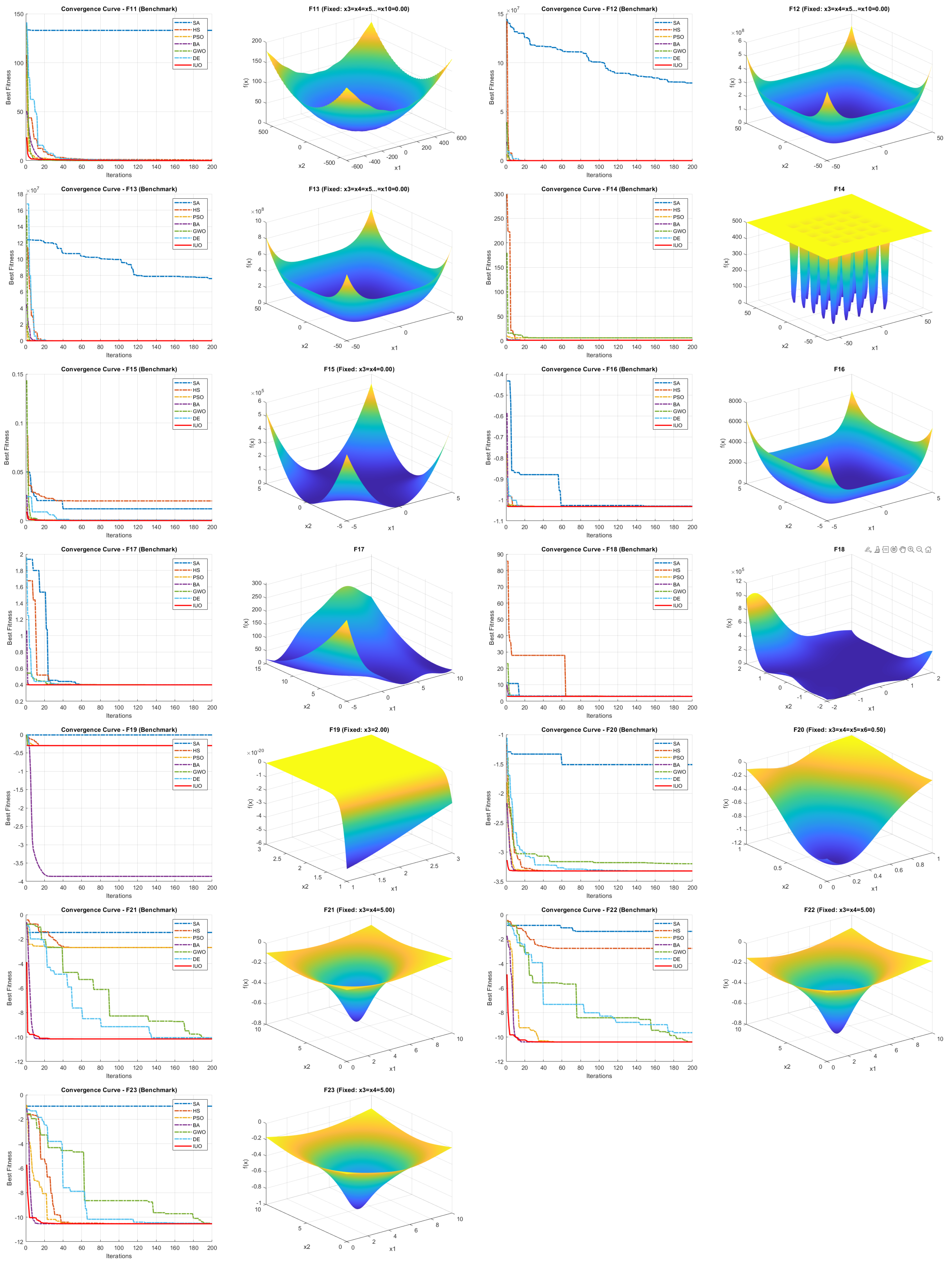
Figure 6.
Pressure vessel design problem
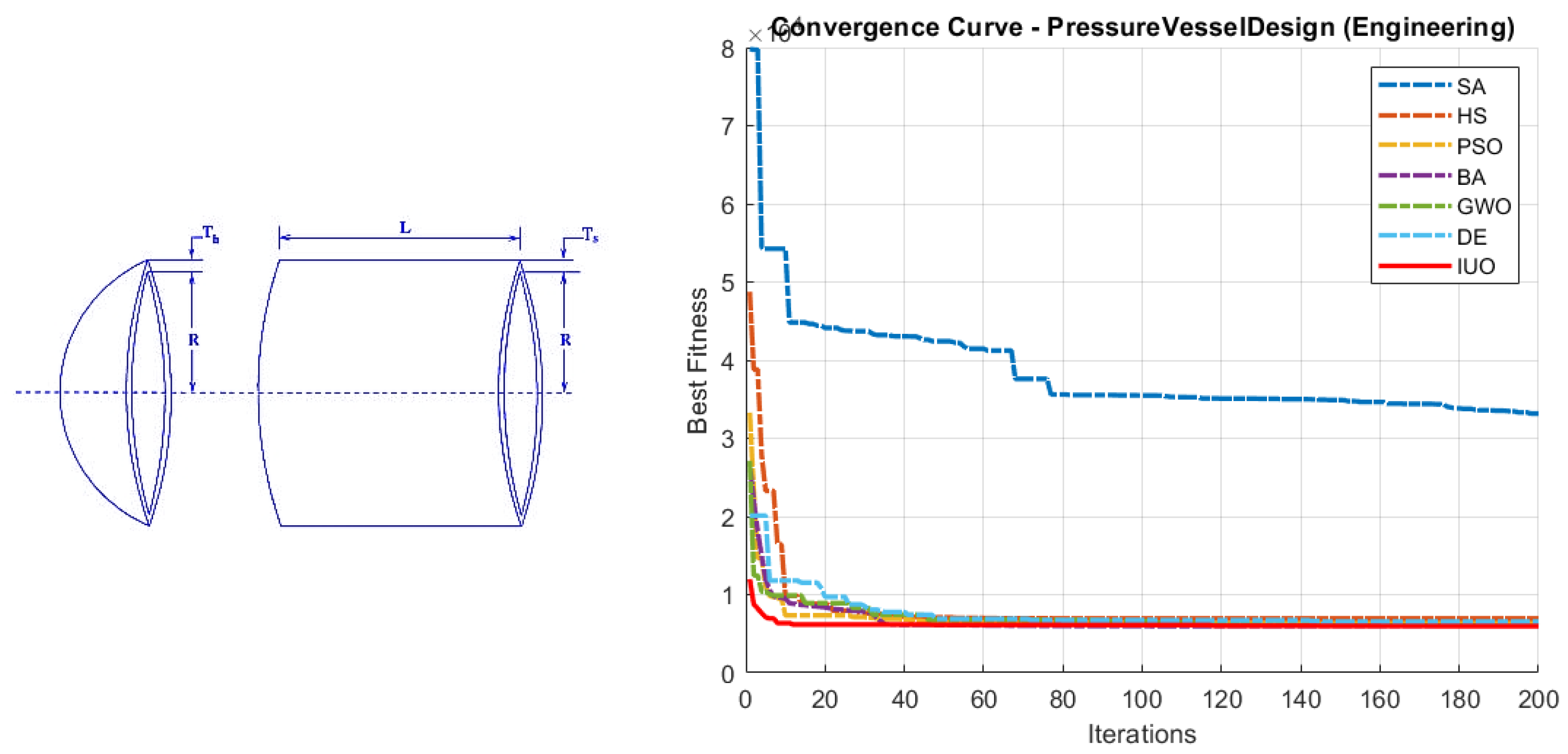
Figure 7.
Welded beam problem
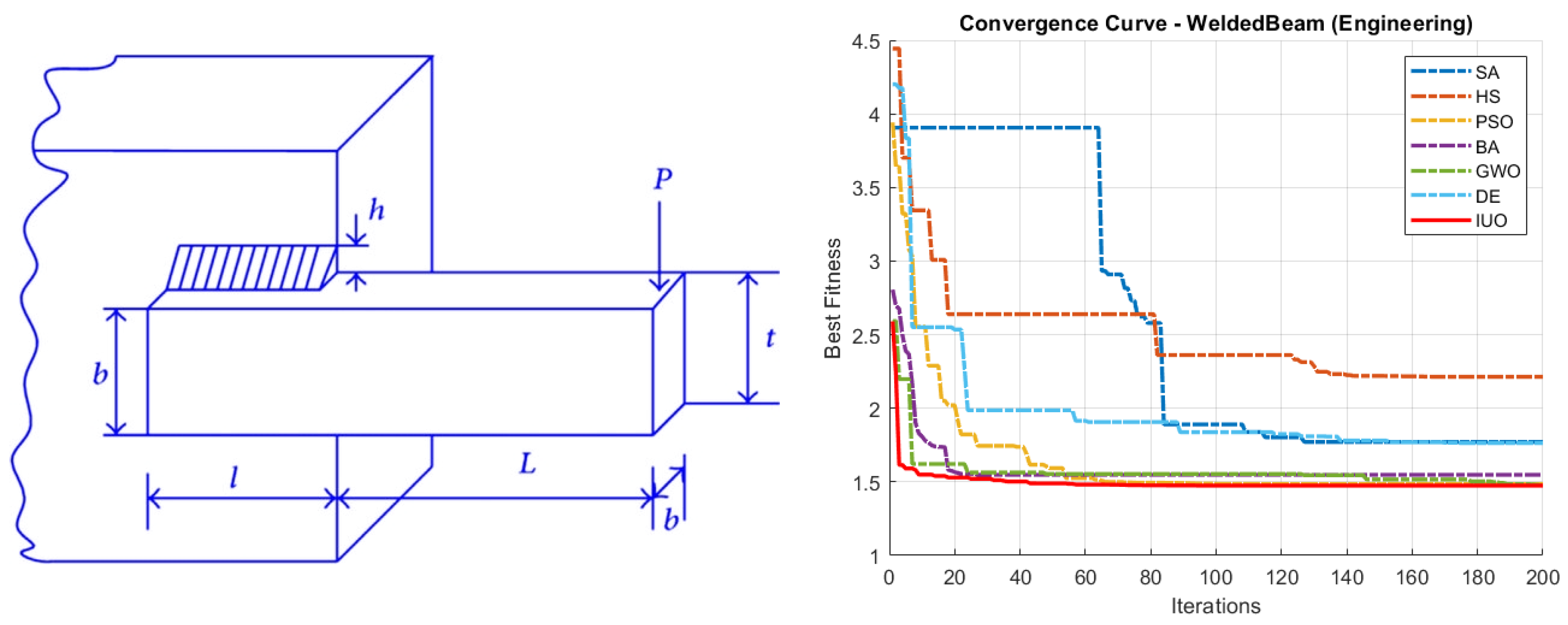
Figure 8.
Three bar truss problem

Figure 9.
Gear train design problem
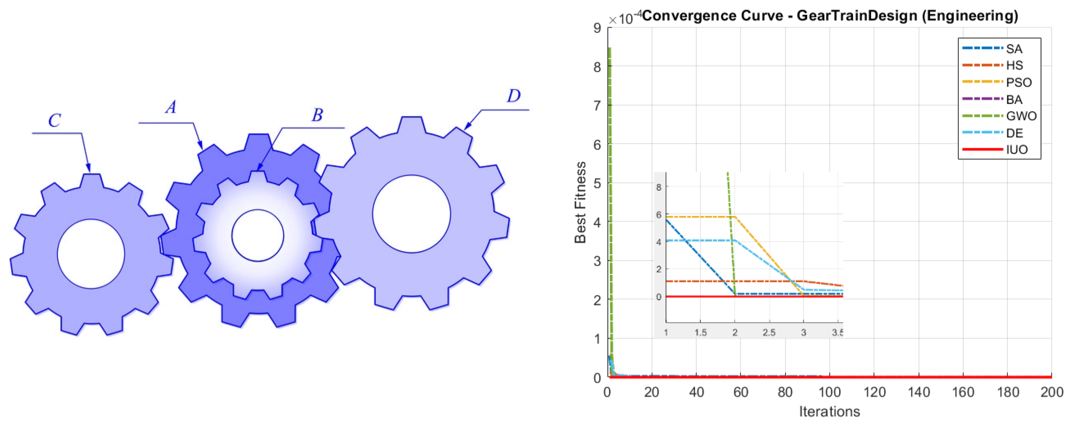
Figure 10.
Spring design problem
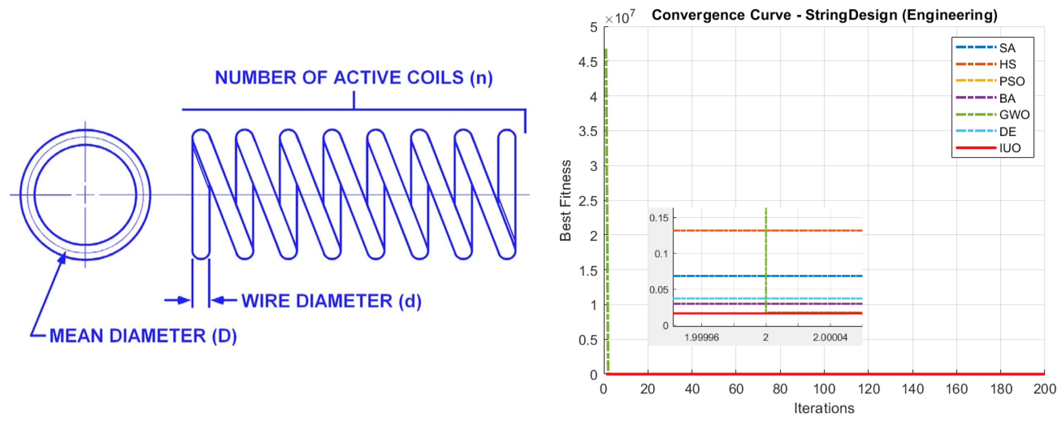
Table 2.
Results for Pressure Vessel Design problem
| Algorithm | Mean | Std. Dev. | Min | Max | Time (s) |
|---|---|---|---|---|---|
| SA | 8934.096009 | 5379.441859 | 6102.836946 | 34650.96102 | 0.00235192 |
| HS | 6790.011332 | 368.3340944 | 6036.090638 | 7346.984089 | 0.202283243 |
| PSO | 6200.74739 | 232.4154512 | 5881.316468 | 6637.982622 | 0.134126303 |
| BA | 6067.60585 | 180.7718386 | 5886.738462 | 6592.957942 | 1.428194373 |
| GWO | 6096.292211 | 297.670369 | 5904.78428 | 7042.994771 | 0.102271043 |
| DE | 6364.532374 | 271.8178418 | 5931.235144 | 7100.692009 | 0.243234097 |
| IUO | 6014.536263 | 123.7783467 | 5880.800346 | 6287.598842 | 0.54142888 |
Table 3.
Results for Welded Beam Design Optimization problem
| Algorithm | Mean | Std. Dev. | Min | Max | Time (s) |
|---|---|---|---|---|---|
| SA | 2.726332768 | 0.736277131 | 1.706098713 | 4.808994011 | 0.00304622 |
| HS | 2.502389078 | 0.402186416 | 1.727371997 | 3.386773788 | 0.159954053 |
| PSO | 1.481628215 | 0.027117542 | 1.473036236 | 1.59272088 | 0.136003083 |
| BA | 1.626826717 | 0.094913048 | 1.481506664 | 1.837726847 | 1.735639073 |
| GWO | 1.481008445 | 0.003224352 | 1.474313901 | 1.489479962 | 0.127010523 |
| DE | 1.728060364 | 0.146277831 | 1.545375391 | 2.110841679 | 0.259273447 |
| IUO | 1.478015882 | 0.00433651 | 1.473081887 | 1.48965118 | 0.67622714 |
Table 4.
Results for Three Bar Truss Design Optimization problem
| Algorithm | Mean | Std. Dev. | Min | Max | Time (s) |
|---|---|---|---|---|---|
| SA | 267.3399544 | 3.29874237 | 264.0909693 | 275.7540047 | 0.002147237 |
| HS | 264.7270402 | 1.478990223 | 263.9175254 | 271.3530086 | 0.1555674 |
| PSO | 263.8965192 | 0.001035261 | 263.8958434 | 263.9007192 | 0.128003677 |
| BA | 263.9038454 | 0.012472964 | 263.8958439 | 263.9457486 | 1.321511923 |
| GWO | 263.90833 | 0.010530054 | 263.8963363 | 263.9440778 | 0.086289453 |
| DE | 263.8977816 | 0.001126223 | 263.8959916 | 263.9011487 | 0.24197931 |
| IUO | 263.8969424 | 0.001394304 | 263.8958494 | 263.9026046 | 0.862995297 |
Table 5.
Results for Gear Train Design Problem
| Algorithm | Mean | Std. Dev. | Min | Max | Time (s) |
|---|---|---|---|---|---|
| SA | 0.000509202 | 0.001637867 | 3.44E-10 | 0.0083914 | 0.000878097 |
| HS | 1.86E-11 | 2.37E-11 | 9.36E-14 | 8.34E-11 | 0.116018317 |
| PSO | 1.79E-17 | 9.52E-17 | 0 | 5.22E-16 | 0.085457267 |
| BA | 7.21E-21 | 1.24E-20 | 9.76E-24 | 5.95E-20 | 0.597746617 |
| GWO | 2.28E-11 | 5.40E-11 | 2.73E-16 | 2.23E-10 | 0.027368293 |
| DE | 1.07E-10 | 2.16E-10 | 1.24E-14 | 9.63E-10 | 0.153666097 |
| IUO | 5.33E-14 | 9.01E-14 | 1.52E-16 | 3.87E-13 | 0.048425533 |
Table 6.
Results for Spring Design Optimization problem
| Function | Algorithm | Mean | Std | Min | Max |
|---|---|---|---|---|---|
| SA | 13456289.72 | 57457173.9 | 0.012954364 | 307083379.2 | 0.004133583 |
| HS | 0.016263369 | 0.001318016 | 0.013328348 | 0.018490406 | 0.157625823 |
| PSO | 0.013692453 | 0.001413855 | 0.012668477 | 0.017538936 | 0.137023597 |
| BA | 0.012666743 | 3.01E-06 | 0.012665262 | 0.01268011 | 1.502232433 |
| GWO | 0.012898701 | 0.000293568 | 0.012700051 | 0.013812856 | 0.13530739 |
| DE | 0.013185465 | 0.000265595 | 0.01282546 | 0.014046053 | 0.27604001 |
| IUO | 0.012827862 | 0.000270974 | 0.012670522 | 0.014062775 | 0.591337073 |
Disclaimer/Publisher’s Note: The statements, opinions and data contained in all publications are solely those of the individual author(s) and contributor(s) and not of MDPI and/or the editor(s). MDPI and/or the editor(s) disclaim responsibility for any injury to people or property resulting from any ideas, methods, instructions or products referred to in the content. |
© 2025 by the authors. Licensee MDPI, Basel, Switzerland. This article is an open access article distributed under the terms and conditions of the Creative Commons Attribution (CC BY) license (http://creativecommons.org/licenses/by/4.0/).
Copyright: This open access article is published under a Creative Commons CC BY 4.0 license, which permit the free download, distribution, and reuse, provided that the author and preprint are cited in any reuse.


