MRBMO: An Enhanced RBMO Algorithm For Solving Numerical Optimization Challenges

1. Introduction

In the field of optimization, metaheuristic algorithms have received widespread attention due to their effectiveness and applicability in solving complex multimodal problems. Metaheuristic algorithms are an improvement of heuristic algorithms and are a combination of random algorithms and local search algorithms. These algorithms are used to solve complex optimization problems by performing global search and local exploration to find the optimal or near-optimal solution. The core of metaheuristic algorithms lies in exploration and exploitation. Exploration refers to the process of thoroughly exploring the entire search space since the optimal solution may exist at any position within the space. Exploitation, on the other hand, focuses on utilizing the available information as much as possible. In most cases, there is a certain correlation between the optimal solutions, and by exploiting these correlations, the algorithm can gradually adjust and evolve from an initial solution to an optimal solution. The main advantage of metaheuristic algorithms is their ability to handle complex, nonlinear problems without requiring assumptions about the specific model of the problem. Although metaheuristic algorithms cannot guarantee a global optimal solution for an optimization problem, they are capable of quickly finding or approximating the optimal solution within a given timeframe.

Over the past few decades, various metaheuristic algorithms have been developed. The Simulated Annealing (SA) algorithm, proposed by Metropolis in 1953, is based on the analogy between the process of solving an optimization problem and the thermal equilibrium problem in statistical thermodynamics. The aim is to find the global or near-optimal solution by simulating the annealing process of a high-temperature object [24]. The Genetic Algorithm (GA), first proposed by John Holland in 1975, is based on Darwin’s theory of evolution and Mendel’s genetics. It uses methods such as reproduction, mutation, and competition among individuals in a population to exchange information and perform a survival-of-the-fittest approach, gradually approaching the optimal solution [2]. The Ant Colony Optimization (ACO) algorithm, proposed by Dorigo et al. in 1991, is a random search algorithm that simulates the food foraging process of real ants in nature [3]. In 1995, American psychologist Kennedy and electrical engineer Eberhart proposed the Particle Swarm Optimization (PSO) algorithm, inspired by the foraging behavior of birds [1]. Due to their excellent optimization ability and versatility, metaheuristic algorithms have been widely applied in various fields such as robot path planning, job shop scheduling, neural network parameter optimization, and feature selection. However, many traditional metaheuristic algorithms, such as PSO, GA, and ACO, often face issues such as getting trapped in local optima and slow convergence when dealing with complex problems. To address these challenges, researchers have attempted to integrate various improvement strategies into basic metaheuristic algorithms, including hybrid algorithms, enhanced exploration-exploitation balance methods, and the introduction of new biological behavior models.

In 2018, Guojiang Xiong et al. proposed the improved whale optimization algorithm (IWOA) with a novel search strategy for solving solar photovoltaic model parameter extraction problems [36]. In 2019, Qiang Tu et al. introduced the Multi-strategy Ensemble Grey Wolf Optimizer (MEGWO) by incorporating global best-guided strategies and adaptive collaborative strategies into the Grey Wolf Optimizer (GWO), aiming to overcome the limitations of the single search strategy in traditional GWO for solving various function optimization problems [37]. In 2023, Ya Shen et al. proposed an improved whale optimization algorithm based on multi-population evolution (MEWOA). The algorithm divides the population into three sub-populations based on individual fitness and assigns different search strategies to each sub-population. This multi-population cooperative evolution strategy effectively enhances the algorithm’s search capability [38]. In 2024, Ying Li et al. proposed the Improved Sand Cat Swarm Optimization algorithm (VF-ISCSO) based on virtual forces and a nonlinear convergence strategy. VF-ISCSO demonstrated significant advantages in enhancing the coverage range of wireless sensor networks [39]. These outstanding algorithms, by integrating various novel improvement strategies, offer new insights into the enhancement of metaheuristic algorithms.

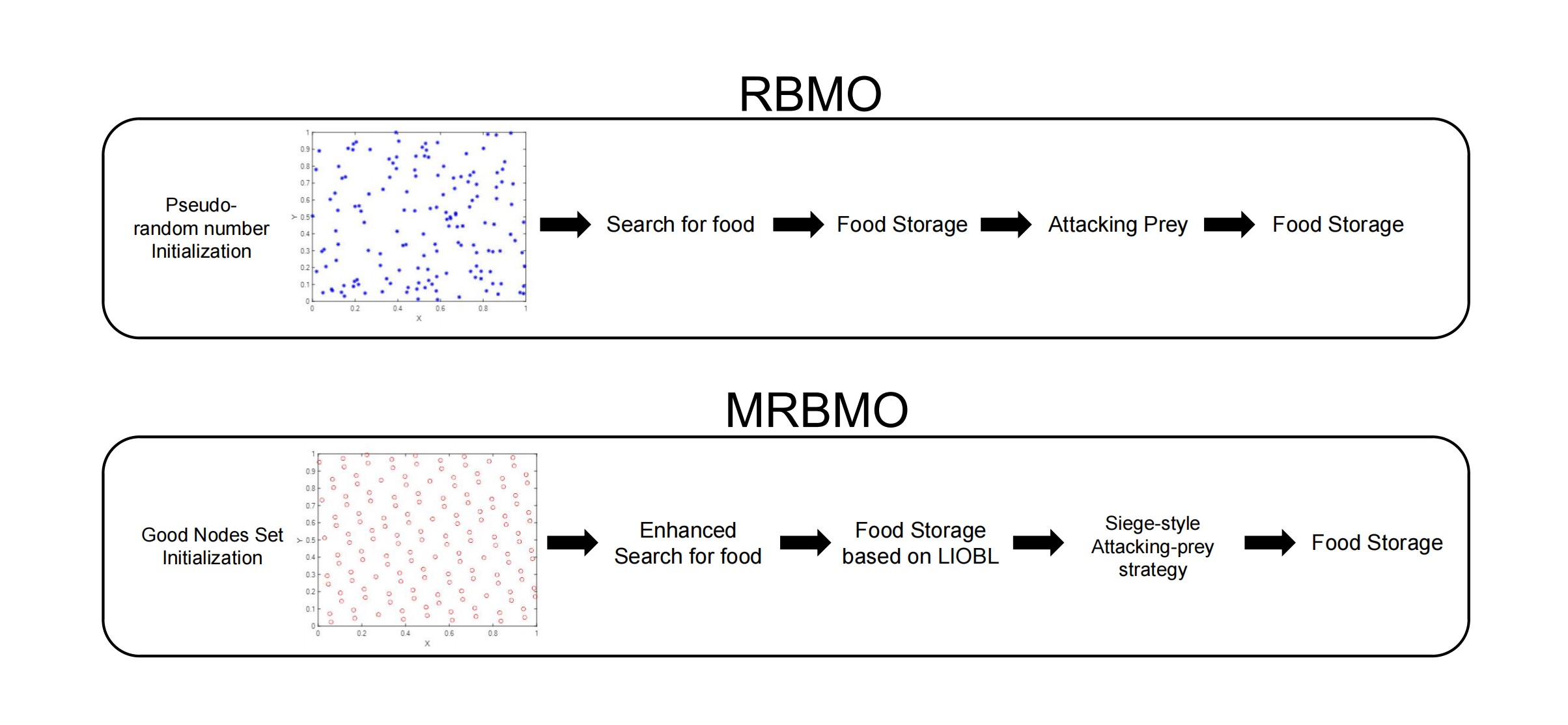
The Red-Billed Blue Magpie Optimization (RBMO) algorithm is a novel metaheuristic algorithm inspired by the foraging behavior and social cooperation characteristics of the red-billed blue magpie [12]. RBMO demonstrates significant advantages in global search, population diversity, and ease of implementation. However, it still exhibits limitations in solution accuracy and convergence speed, particularly when dealing with complex multimodal problems, where it struggles to quickly approach the optimal solution. To address these challenges, this paper proposes an enhanced RBMO algorithm (MRBMO). MRBMO was improved by integrating Good Nodes Set Initialization, an Enhanced Search-for-food Strategy a newly designed Siege-style Attacking-prey Strategy snd Lens-Imaging Opposition-Based Learning (LIOBL). These strategies enhance the local search ability of RBMO and accelerate its convergence speed.

2. Research Work on Antenna Design

Adegboye et al. introduced the Honey Badger Algorithm (HBA) for antenna design optimization, demonstrating the algorithm’s effectiveness in enhancing antenna performance through specific cases [12]. The improvements were evident in key metrics such as gain and bandwidth. They compared the performance of various algorithms in antenna design, highlighting the advantages of the new algorithm in addressing particular design challenges. Park et al. proposed a method for optimizing antenna placement in single-cell and dual-cell distributed antenna systems (DAS) to maximize the lower bounds of expected signal-to-noise ratio (SNR) and expected signal-to-leakage ratio (SLR) [1]. The results indicated that the DAS using the proposed gradient ascent-based algorithm outperforms traditional centralized antenna systems (CAS) in terms of capacity, especially in dual-cell environments, effectively reducing interference and improving system performance. Jiang et al. designed a multi-band pixel antenna using genetic algorithms and N-port characteristic modal analysis, which operates effectively across the 900 MHz, 1800 MHz, and 2600 MHz frequency bands [13]. The effectiveness of the genetic algorithm in antenna design optimization was validated by monitoring changes in the objective function. Yang Zhao et al. proposed an optimization design method for dual-band tag antennas based on a multi-population genetic algorithm, overcoming the inefficiencies of traditional simulation and parameter tuning experiments in determining optimal size parameters [14]. The optimized UHF antenna achieved near-ideal input impedance at 915 MHz, resulting in good impedance matching with the chip. The size of the optimized dual-band tag antenna was significantly reduced compared to existing designs. Cai Jiaqi et al. presented a self-optimization method for base station antenna azimuth and downtilt angles based on the Artificial Bee Colony algorithm [15]. Experimental results provided the optimal azimuth and downtilt angles for base station antennas, improving coverage effectiveness for user devices, particularly in weak coverage areas. Fengling Peng et al. developed an antenna optimization framework based on Differential Evolution (DE), customized decision trees, and Deep Q-Networks (DQN) [16]. Experimental results showed that this hybrid strategy-based framework achieves superior antenna design solutions with fewer simulation iterations. Meta-heuristic algorithm plays an important role in antenna design.

3. Research Work on Engineering Design Optimization

In early engineering design, the concept of "optimization" was typically absent. Engineering design relied heavily on manual calculations and intuitive judgment. In the early 20th century, with the development of mathematical optimization theory, optimization tools gradually began to be introduced into engineering design. The initial optimization methods were based on classical mathematical analysis, such as calculus, to derive the optimal solution through analytical reasoning. In the 1940s, George Dantzig and others proposed Linear Programming (LP), which provided a mathematical foundation for optimization and was widely applied in economics, transportation, and resource allocation problems. With the emergence of nonlinear systems, engineering design faced more complex optimization problems, necessitating new mathematical tools. Numerical methods, such as Newton’s method and gradient descent, were introduced and applied to engineering optimization. However, due to the lack of powerful computational tools, engineering design remained a time-consuming and complex process, mostly relying on simplified assumptions to solve problems. From the 1950s to the 1970s, advancements in computers drove the computerization of engineering design optimization. Engineers began to use computer programs, achieving breakthroughs particularly in Finite Element Analysis (FEA) and Dynamic Programming (DP). The Finite Element Method (FEM) helped address stress and deformation problems in complex structures, while Dynamic Programming was widely applied in control and scheduling problems. Despite these advancements, early computer-aided design still mainly used deterministic mathematical methods for solutions, which were applicable only to specific types of problems. When facing large-scale, complex engineering problems, the computational effort and difficulty of solving remained significant. By the 1980s, as the scale and complexity of engineering design problems increased, traditional mathematical optimization methods gradually became inadequate for handling high-dimensional, nonlinear, and complex-constrained optimization issues. Researchers shifted towards metaheuristic algorithms (such as Simulated Annealing, Genetic Algorithms, Particle Swarm Optimization, etc.). These algorithms could avoid local optima and offer better optimization solutions, especially for complex, irregular, or high-dimensional problems. The improvement in computer hardware performance also allowed these algorithms to handle larger-scale optimization problems. In the 2010s, the development of Artificial Intelligence (AI) and Deep Learning (DL) provided new options for engineering design optimization. Neural networks could assist design optimization by learning from large amounts of historical data. However, AI has the disadvantage of long training times and dependence on large datasets, which may yield poor results when data is scarce. AI is also constrained by existing mathematical models, whereas metaheuristic algorithms, due to their robustness, can maintain high optimization performance across various complex problems without relying on mathematical models or derivative information, demonstrating strong adaptability. Therefore, metaheuristic algorithms remain the primary solution method for engineering design optimization.

4. Arrangement of the Rest of the Paper

Chapter 5 primarily presents the main contributions of this study. Chapter 6 introduces the specific principles of the RBMO algorithm, along with its advantages and disadvantages. Chapter 7 introduces the proposed MRBMO. In Chapter 8, we will test the performance of MRBMO through a series of experiments. In Chapter 9, various metaheuristic algorithms and MRBMO will be simulated and tested on different engineering design optimization problems and antenna S-parameter optimization suites to verify the practicality of MRBMO.

5. contributions of This Study

By integrating Good Nodes Set Initialization, an Enhanced Search-for-food Strategy, a newly designed Siege-style Attacking-prey Strategy and Lens-Imaging Opposition-Based Learning (LIOBL), we proposed a novel optimizer MRBMO for solving real-world challenges. By performing a ablation study, we evaluated the effectiveness of each strategy. By comparing MRBMO with other excellence metaheuristic algorithms on the classical benchmark functions, we validated the outstanding performance of MRBMO. In a subsequent series of simulation experiments, MRBMO demonstrated excellent optimization ability and good convergence, proving that MRBMO can be used in the real world to solve various numerical optimization problems.

6. Red-Billed Blue Magpie Optimization Algorithm

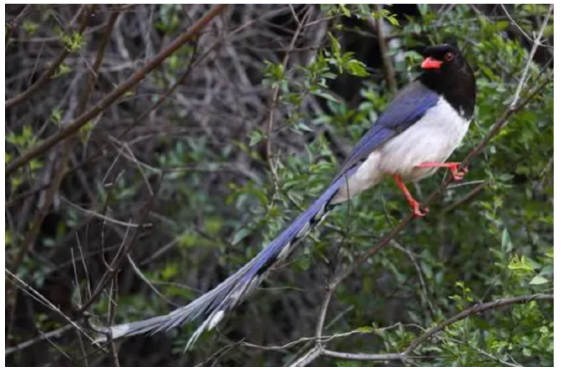
The red-billed blue magpie is a bird that lives mainly in Asia and is common in China, India, and Myanmar, as shown in Figure 1, which depicts the red-billed blue magpie, which is characterized by its large size, bright blue plumage, and distinctive red beak. The red-billed blue magpie feeds mainly on insects, small vertebrates, plants, etc., and has relatively abundant hunting behavior. When foraging, red-billed blue magpies use a combination of jumping, ground walking and searching for food on branches.

Red-billed blue magpies show high activity levels in the early morning and evening, often gathering in small groups of 2-5 or even more than 10 individuals. They are involved in co-operative hunting. For example, a magpie may find fruit or an insect which it will then attract other members to share. This allows them to co-operate in catching large insects or small vertebrates, and group action can help them overcome the defence mechanisms of their prey. Magpies also store some food for later use. To prevent other birds or animals from stealing it, they hide food in places such as tree holes, branches and rock crevices.

Overall, red-billed blue magpies are flexible predators that acquire and store food in a variety of ways, as well as showing sociality and cooperation in their hunting behaviour. Inspired by this, Shengwei Fu et al. proposed a new metaheuristic algorithm, the Red-billed Blue Magpie Optimization algorithm (RBMO) in 2024 [4]. When RBMO deals with complex problems, each optimization problem has its own objective function, the solution space consists of the values of an objective function. The mission for RBMO is to search the optimal or suboptimal solution in the solution space. In each iteration, RBMO will randomly generate N individuals in the solution space. The individuals are called search agents, and they will move by imitating the behavior of the red-billed blue magpie in searching for prey, attacking prey or storing food. Meanwhile, they will update their position and the position is called a solution or the fitness of an objective function. After many iterations, they can find the optimal or suboptimal solution in the solution space.

6.1. Search for Food

In red-billed blue magpies’ search-for-food stage, they use a variety of methods such as hopping on the ground, walking or searching for food resources in trees. The whole flock will be devided into small groups of 2-5 individuals or in clusters of 10 or more to search for food.

RBMO imitates their search-for-food behavior in small groups as follows,

$$X^i(t+1)=X^i\left(t\right)+({\displaystyle \frac{1}{p}}·\sum _{m=1}^p{X}^m\left(t\right)-X^{rs}\left(t\right))·Ran{d}_1$$

(1)

where t represents the current iteration number; $X^i\left(t\right)$ represents the location of $t^{th}$ new search agent; p is a random integer between 2 and 5, representing the number of red-billed blue magpies in a population of 2 to 5 randomly selected from all searched individuals; $X^M$ represents the $m^{th}$ randomly selected individual; $X^i$ represents the $i^{th}$ individual; and $X^{rs}$ represents the randomly selected search agent in the current iteration; $Ran{d}_1$ is a random number range from [0,1].

Also, RBMO imitates their search-for-food behavior in clusters as follows,

$$X^i(t+1)=X^i\left(t\right)+({\displaystyle \frac{1}{q}}·\sum _{m=1}^q{X}^m\left(t\right)-X^{rs}\left(t\right))·Ran{d}_2$$

(2)

where q is a random integer between 10 and n, representing the number of red-billed blue magpies in a population of 10 to n randomly selected from all searched individuals; $Ran{d}_2$ is a random number range from [0,1].

The whole Search-for-food Strategy is modeled below.

$$\begin{array}{c}\hfill X^i(t+1)=X^i\left(t\right)+({\displaystyle \frac{1}{p}}·\sum _{m=1}^p{X}^m\left(t\right)-X^{rs}\left(t\right))·Ran{d}_1,rand<\epsilon \end{array}$$

(3)

$$\begin{array}{c}\hfill X^i(t+1)=X^i\left(t\right)+({\displaystyle \frac{1}{q}}·\sum _{m=1}^q{X}^m\left(t\right)-X^{rs}\left(t\right))·Ran{d}_2,rand\ge \epsilon \end{array}$$

(4)

6.2. Attacking Prey

When attacking prey, red-billed blue magpies show a high degree of hunting proficiency and co-operation. Red-billed blue magpies use tactics such as rapid pecking, jumping to catch prey or flying to catch insects, and they usually move in small groups of 2-5 or in clusters of 10 or more to increase hunting efficiency.

RBMO imitates red-billed blue magpies’ attacking-prey behavior in small groups as follows,

$$X^i(t+1)=X^{food}\left(t\right)+CF·({\displaystyle \frac{1}{p}}·\sum _{m=1}^p{X}^m\left(t\right)-X^i\left(t\right))·Rand{n}_1$$

(5)

where $X^i\left(t\right)$ represents the location of $t^{th}$ new search agent; $X^{food}$ represents the position of the food, which indicates the current optimal solution; p is a random integer between 2 and 5, representing the number of red-billed blue magpies in a population of 2 to 5 randomly selected from all searched individuals; $Rand{n}_1$ denotes the random number used to generate the standard normal distribution (mean 0, standard deviation 1); $CF$ is the step control factor, calculated as in Eq 6.

$$CF={\left(1-{\displaystyle \frac{t}{T}}\right)}^{(2·{\displaystyle \frac{t}{T}})}$$

(6)

where t represents the current number of iterations; T represents the maximum number of iterations.

RBMO imitates red-billed blue magpies’ attacking-prey behavior in clusters as follows,

$$X^i(t+1)=X^{food}\left(t\right)+CF·({\displaystyle \frac{1}{q}}·\sum _{m=1}^q{X}^m\left(t\right)-X^i\left(t\right))·Rand{n}_2$$

(7)

where q is a random integer between 10 and n, representing the number of red-billed blue magpies in a population of 10 to n randomly selected from all searched individuals; $Rand{n}_2$ denotes the random number used to generate the standard normal distribution (mean 0, standard deviation 1).

The Attacking prey is modeled below.

$$\begin{array}{c}\hfill X^i(t+1)=X^{food}\left(t\right)+CF·({\displaystyle \frac{1}{p}}·\sum _{m=1}^p{X}^m\left(t\right)-X^i\left(t\right))·Rand{n}_1,rand<\epsilon \end{array}$$

(8)

$$\begin{array}{c}\hfill X^i(t+1)=X^{food}\left(t\right)+CF·({\displaystyle \frac{1}{q}}·\sum _{m=1}^q{X}^m\left(t\right)-X^i\left(t\right))·Rand{n}_2,rand\ge \epsilon \end{array}$$

(9)

6.3. Food Storage

As well as searching for food and attacking food, red-billed blue magpies store excess food in tree holes or other hidden places for future consumption, ensuring a steady supply of food in times of shortage.

RBMO imitates the storing-food behavior of red-billed blue magpies. And the formula for storing food is shown in Eq 10.

$$X^i(t+1)=\left\{\begin{array}{cc}{X}^i\left(t\right)\hfill & \mathrm{if}fitnes{s}_{old}^i>fitnes{s}_{new}^i\hfill \\ X^i(t+1)\hfill & else\hfill \end{array}\right.$$

(10)

where $fitnes{s}_{old}^i$ and $fitnes{s}_{new}^i$ denote the fitness values before and after the position update of the $i^{th}$ red-billed blue magpie respectively.

6.4. Initialization

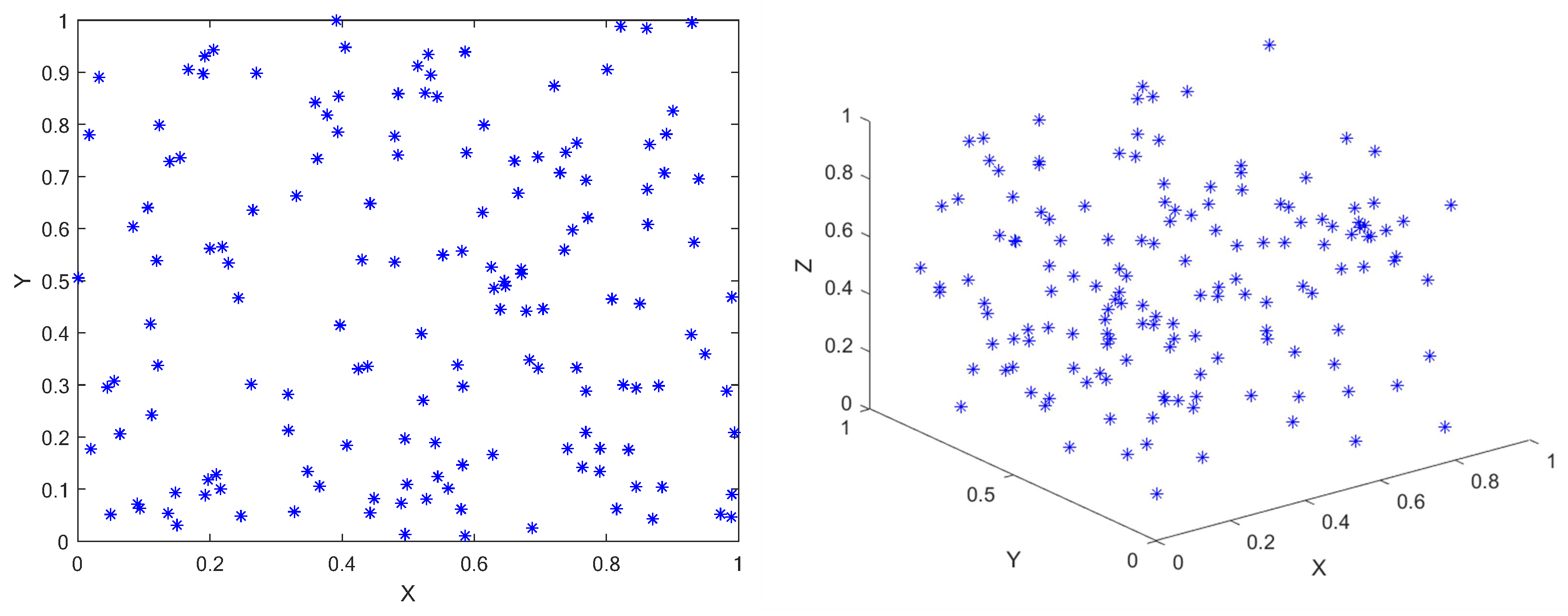
Like most metaheuristic algorithms, RBMO uses Pseudo-random number initialization for population initialization. This approach, while simple and direct, often results in poor diversity and uneven distribution of solutions, which can lead to inefficiency in the search process. Figure 2 is the population initialized by Pseudo-random number method.

$$X_{i,j}=(ub-lb)·Rand+lb$$

(11)

where $X_{i,j}$ is randomly produced population; $ub$ and $lb$ are the upper limit and lower limit of the problem; $Rand$ is a random number between 0 and 1.

6.5. Workflow of RBMO and Its Analysis

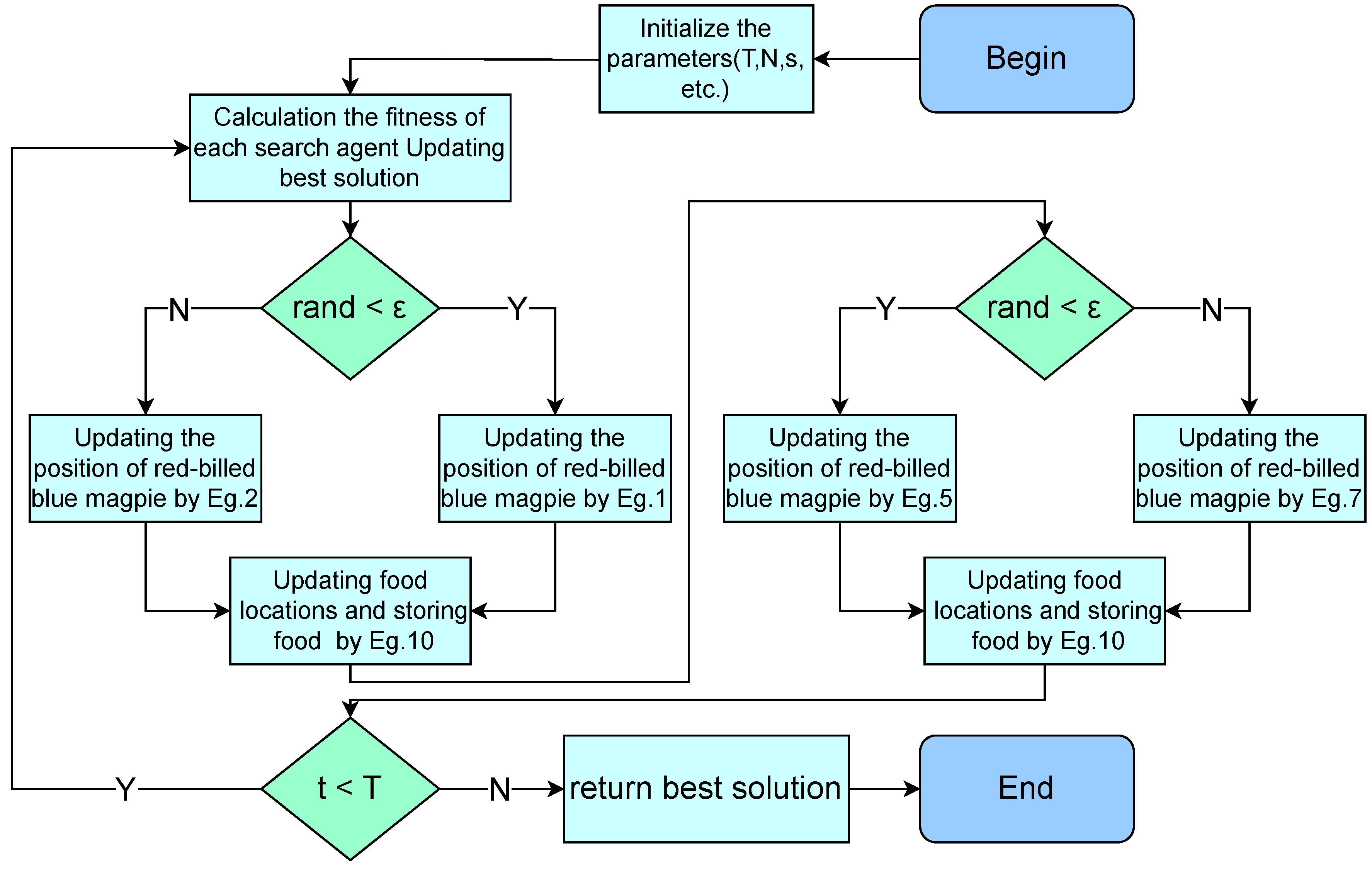
The workflow of RBMO is provided in Figure 3.

As a new biologically metaheuristic algorithm, RBMO has significant advantages in global search, population diversity and simplicity of implementation.The update mechanism of RBMO increases the breadth and diversity of the search by randomly selecting the mean values of multiple individuals for updating, which enables it to cover a larger search space, thus effectively avoiding falling into a local optimum. Secondly, the algorithm structure of RBMO is simple and easy to implement, which is suitable for the rapid solution of different fields and problems. In addition, by randomly selecting individuals and mean updating strategies, RBMO is able to adapt to different types and sizes of optimization problems, showing good stability and adaptability.

However, RBMO also has some limitations, especially in the local search ability and convergence speed. As the attacking-prey strategy of RBMO is relatively monotonous, which leads to its insufficient local search ability when facing complex and multi-peak problems, it is difficult to approach the optimal solution quickly. In addition, the convergence speed of RBMO is relatively slow, and more iterations are needed to find a better solution in the optimization process. These shortcomings limit the effectiveness and efficiency of RBMO application to some extent. In order to solve these problems, enhance the local search capability of RBMO and accelerate the convergence speed, we propose an enhance RBMO, which is called MRBMO.

7. MRBMO

7.1. Good Nodes Set Initialization

The original RBMO uses pseudo-random number method to initialize the population, this method is simple, direct and random, but there are some drawbacks. the randomly generated population, as shown in Figure 2, is not uniformly distributed throughout the solution space, it is very aggregated in some areas and scattered in some areas, which leads to the algorithm’s poor exploitation of the whole search space and low diversity of the population. Therefore, some experts proposed to use chaotic mapping, random wandering, Gaussian distribution and other methods to initialize the population. Later some scholars proposed to use the good nodes set initialization.

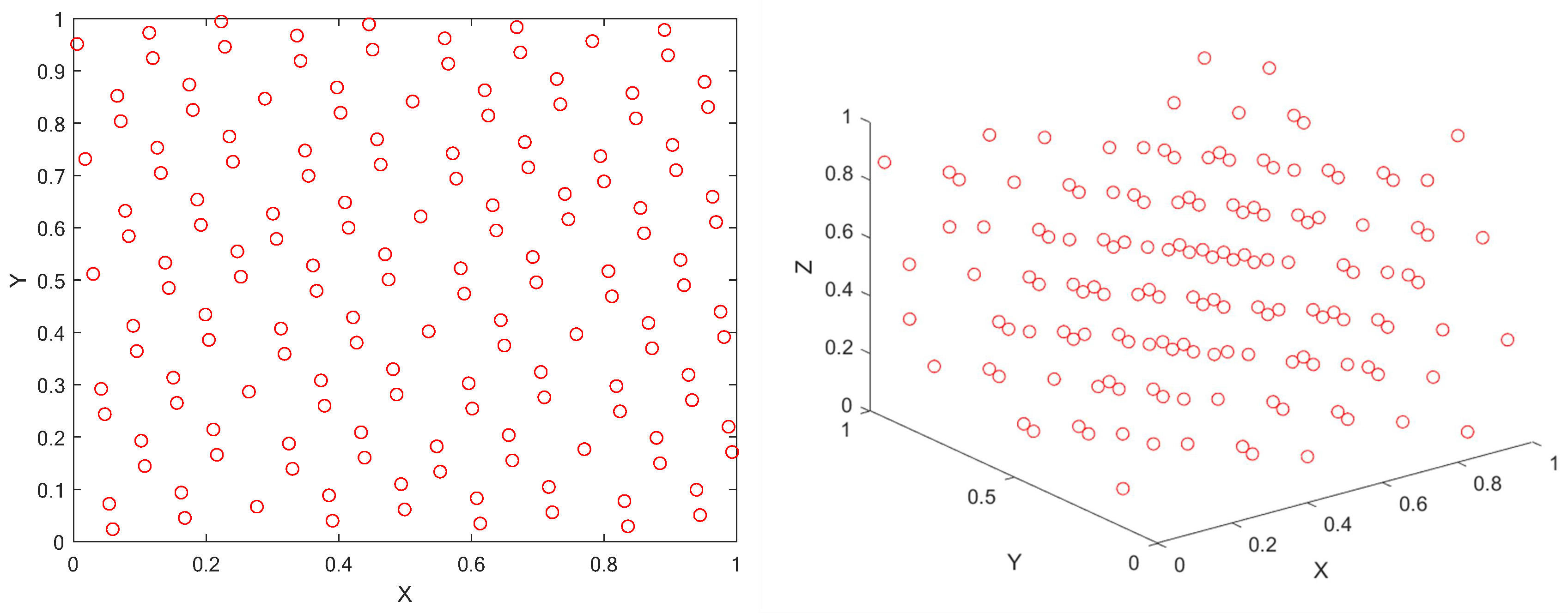
The theory of Good Nodes Set was first proposed by the famous Chinese mathematician Loo-keng Hua. Good Nodes Set is a method used to cover a multidimensional space uniformly, aiming to improve the quality of initialized populations. Compared with the traditional initialization method, Good Nodes Set initialization, as shown in Figure 4, can better distribute the nodes and improve the diversity of the population, thus providing better initial conditions for the optimization algorithm. This method is also effective in high dimensional spaces.

Assuming that $U^D$ is a unit cube in the D dimensional Euclidean space, and assuming that r is a parameter, the set of canonical nodes $P_r^M$ has the form shown in Eq 12:

$$P_r^M=\{p\left(k\right)=(\left\{kr\right\},\left\{k{r}^2\right\},\dots ,\left\{k{r}^D\right\})|k=1,2,\dots ,M\}$$

(12)

where {x} represents the fractional part of x; M is the number of points; r is a deviation parameter greater than zero; the constant $C(r,\epsilon )$ is associated only with r and $\epsilon$ is related to and is a constant greater than zero.

This set $P_r^M$ is called Good Nodes Set and each node $p\left(k\right)$ in it is called a Good Node. Assume that the upper and lower bounds of the $i^{th}$ dimension of the search space $x_{max}^i$ are and $x_{min}^i$, then the mapping formula for mapping the Good Nodes Set to the actual search space is:

$$x_k^i=x_{min}^i+p_i\left(k\right)·(x_{max}^i-x_{min}^i)$$

(13)

7.2. Enhanced Search-for-food Strategy

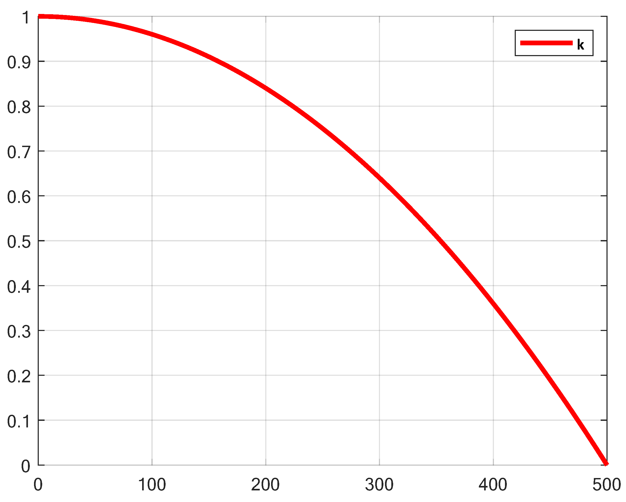
In the original RBMO, the Search-for-food phase relies on the random number and lacks dynamic adjustment, which results in large random fluctuations between the population individuals. Particularly in the later stages of iteration, individuals may still explore with large step sizes, leading to a decrease in search efficiency and affecting convergence accuracy. Therefore, this paper introduces a nonlinear factor k, which enables more thorough exploration in the early stages and more refined development in the later stages. The variation process of k is shown in Figure 5. And the calculation of the nonlinear factor k is as follows:

$$k=1-{\left({\displaystyle \frac{t}{T}}\right)}^2$$

(14)

where t represents the current number of iterations; T represents the maximum number of iterations.

In the early iterations, the value of k is close to 1, which enhances the large step movements between the population individuals, thus improving global exploration ability. In the later iterations, the value of k approaches 0, limiting the movement range of individuals and gradually transitioning towards local exploitation. By introducing the nonlinear factor k, the search intensity of RBMO dynamically decays, naturally balancing exploration and exploitation, thereby improving convergence stability. The Enhanced Search-for-food Strategy addresses the issue of excessive randomness in the search phase of the original algorithm. The Enhanced Search-for-food Strategy is modeled below.

$$\begin{array}{c}\hfill X^i(t+1)=X^i\left(t\right)+k·({\displaystyle \frac{1}{p}}·\sum _{m=1}^p{X}^m\left(t\right)-X^{rs}\left(t\right)),rand<\epsilon \end{array}$$

(15)

$$\begin{array}{c}\hfill X^i(t+1)=X^i\left(t\right)+k·({\displaystyle \frac{1}{q}}·\sum _{m=1}^q{X}^m\left(t\right)-X^{rs}\left(t\right)),rand\ge \epsilon \end{array}$$

(16)

7.3. Siege-Style Attacking-prey Strategy

7.3.1. HHO

The original RBMO algorithm is prone to getting stuck in local optima because the average position induces a contraction effect on the dynamic range of the population, limiting further exploration of the search space. Furthermore, in the original RBMO algorithm, the strategy for attacking prey relies on the average position of the red-billed blue magpie individuals. This updating mechanism may lead to a decrease in population diversity, resulting in slower convergence and reduced accuracy and efficiency of the search, thus hindering further optimization. Therefore, inspired by the Harris Hawk Optimization (HHO) algorithm, this paper introduces the concept of HHO into the prey attack phase of RBMO, proposing the Siege-style Attacking-prey Strategy.

The Harris Hawk Optimization (HHO), introduced by Ali Asghar Heidari et al. in 2019, is a novel bio-inspired optimization algorithm. The HHO algorithm simulates the diverse hunting strategies of Harris hawks, allowing HHO to perform efficient global search in a larger solution space while reducing the likelihood of falling into local optima. At the development stage, the HHO algorithm fine-tunes the position of prey to perform local search, thereby finding better solutions in the local regions of the solution space. We draw inspiration from the following position updating strategy of HHO.

$$X(t+1)=\Delta X\left(t\right)-E·|J·X_{rabbit}\left(t\right)-X\left(t\right)|$$

(17)

$$\Delta X\left(t\right)=X_{rabbit}\left(t\right)-X\left(t\right)$$

(18)

where X is the positions of the Harris hawk at the $t^{th}$ iteration; E is the energy of the prey; J is a prey’s random step while escaping; and $X_{rabbit}$ represents the position of the food, which indicates the current optimal solution.

The Siege-style Attacking-prey Strategy integrates the ideas of HHO, introducing the absolute difference between the prey’s position $X^{food}$ and the red-billed blue magpie individual’s current position $X^i\left(t\right)$, combined with the step size $CF$ to directly adjust the individual’s position update step size. This mechanism helps to guide the red-billed blue magpie individuals more rapidly toward better solutions, refining the local development capability of RBMO in later stages, thereby improving solution accuracy and accelerating convergence speed. Additionally, through the combination of a random factor and nonlinear scaling, the Siege-style Attacking-prey Strategy maintains population diversity during the development phase. With the dynamically adjusted step size $CF$, the attacking behavior of the red-billed blue magpie individuals can adapt to the different search demands at various stages of iteration, enhancing exploration in the early stages and reinforcing exploitation in the later stages. This avoids premature convergence to a single solution and improves the robustness of the algorithm.

7.3.2. Levy Flight

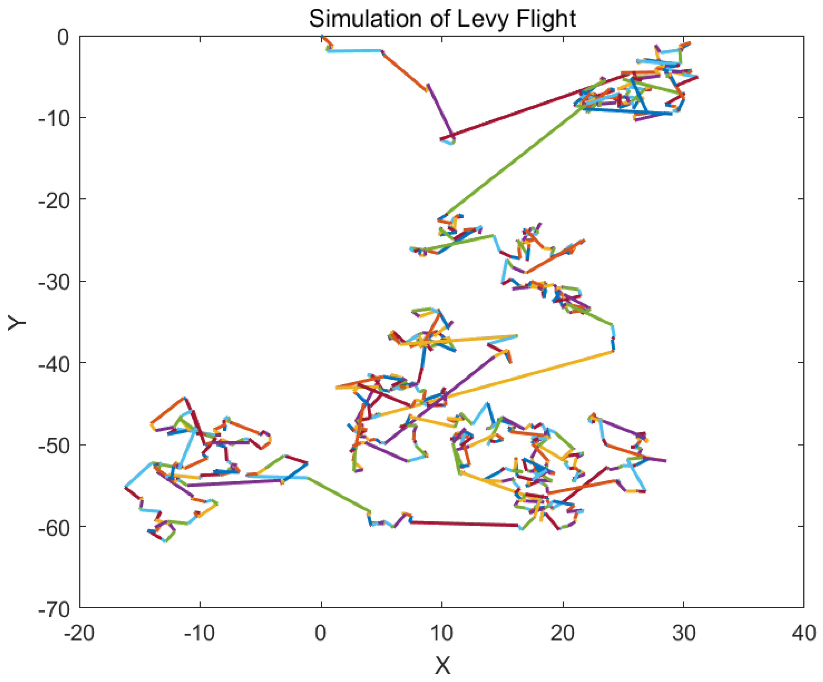
The concept of Levy flight originates from the work of mathematician Paul Levy in the 1920s. Inspired by foraging behavior observed in nature and jump phenomena in complex systems, Levy flight combines short-range exploration with long-range jumps, resembling the foraging paths of predators such as sharks, birds, and insects. Levy flight is a stochastic walk model based on the Levy distribution, with a key characteristic of combining short-distance small steps and long-distance large jumps. This search pattern helps prevent individuals from getting trapped in local dead ends while maintaining the ability to explore the global space. The long jumps in Levy flight allow algorithms to quickly escape local regions, significantly improving the issue of local optima in complex problems. The higher proportion of short-distance small steps enables precise searching within local regions. Figure 6 shows a simulation of Levy flight. The step length $L\left(s\right)$ of Levy flight follows the Levy distribution, calculated as follows:

$$L\left(s\right)={\displaystyle \frac{u}{{\left|\nu \right|}^{\frac{1}{\beta }}}}$$

(19)

where u and $\nu$ are normally distributed; $\beta$=1.5.

$$u\sim \mathcal{N}(0,{\sigma }_u^2)$$

(20)

$$v\sim \mathcal{N}(0,1)$$

(21)

The calculation of ${\sigma }_u$ is given by:

$${\sigma }_u={\left({\displaystyle \frac{\Gamma (1+\beta )·sin\left(\frac{\pi \beta }{2}\right)}{\Gamma \left(\frac{1+\beta }{2}\right)·\beta ·2^{\frac{\beta -1}{2}}}}\right)}^{{\displaystyle \frac{1}{\beta }}}$$

(22)

One of the Siege-style Attacking-prey Strategy is modeled in Eq 23.

$$X^i(t+1)=\Delta X\left(t\right)-CF·|r_1·X^{food}\left(t\right)-X^i\left(t\right)|·L\left(s\right)$$

(23)

where $X^{food}$ represents the position of the food, which indicates the current optimal solution; $CF$ is the step control factor, calculated as in Eq 6; $r_1$ is a the random number between [0, 1]; $\Delta X\left(t\right)$ is calculated in Eq 18; $L\left(s\right)$ is the step size of Levy flight.

7.3.3. Prey-Position-Based Enhanced Guidance

In the original attacking-prey phase, the movement of the red-billed blue magpie individuals relies on both the position of the prey and the average position of the randomly selected red-billed blue magpies. This movement strategy introduces some randomness and bias, which causes individuals to become trapped near suboptimal solutions and prevents them from fully utilizing information about the global optimum, hindering the local exploitation of the RBMO. Therefore, we propose Prey-position-based Enhanced Guidance. In this approach, we replace the average position of the randomly selected red-billed blue magpies with the position of the prey, directly guiding the red-billed blue magpie individuals towards the prey. This helps to reduce the gap between the individuals and the optimal solution. Prey-position-based Enhanced Guidance strengthens the dependency on the optimal position, mitigates the degradation of solution quality due to randomness, and enhances the concentration of local exploitation. Therefore, Prey-position-based Enhanced Guidance, one of the Siege-style Attacking-prey Strategy, is modeled in Eq 24.

$$X^i(t+1)=X^{food}\left(t\right)+CF·(X^{food}\left(t\right)-X^i\left(t\right))·r_2$$

(24)

where $X^{food}$ represents the position of the food, which indicates the current optimal solution; $CF$ is the step control factor, calculated as in Eq 6; $r_2$ is a the random number between [0, 1]. The whole Siege-style Attacking-prey Strategy is modeled below.

$$\begin{array}{cc}\hfill X^i(t+1)& =\Delta X\left(t\right)-CF·|r_1·X^{food}\left(t\right)-X^i\left(t\right)|·L\left(s\right),rand<\epsilon \hfill \end{array}$$

(25)

$$\begin{array}{cc}\hfill X^i(t+1)& =X^{food}\left(t\right)+CF·(X^{food}\left(t\right)-X^i\left(t\right))·r_2,rand\ge \epsilon \hfill \end{array}$$

(26)

7.4. Lens-Imaging Opposition-Based Learning

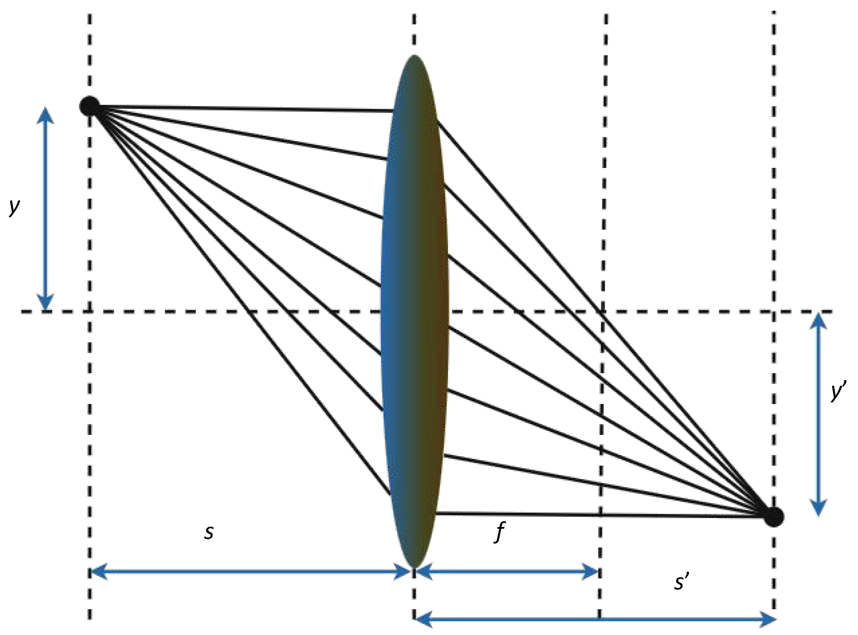
The food storage mechanism in RBMO passively retains better individuals, which may cause the algorithm to hover around local optima. However, the Lens-Imaging Opposition-Based Learning (LIOBL) strategy is more forward-looking. Therefore, we introduce the idea of LIOBL into the food storage mechanism of RBMO. LIOBL increases the diversity of solutions by generating multiple opposite solutions, thereby improving the exploration capability of RBMO in the later stages and enabling it to find solutions closer to the global optimum more quickly. The fundamental idea of Opposition-Based Learning (OBL) is to generate not only neighboring solutions of the current solution during the search process but also its opposite solutions, and then compare the current solution with the opposite solutions to select the better solution. The LIOBL strategy extends OBL by incorporating the concept of reflection, which is shown in Figure 7, where the opposite solutions generated by reflection are used to enhance the coverage of the solution space and improve the global exploration capability of the algorithm [30]. The opposite solutions generated by LIOBL are not only the opposites of the current solution but also include the reflected positions of the opposite solutions in the solution space. The opposition solutionis calculated by Eq 27.

$$X_i^{\prime }={\displaystyle \frac{u_b+l_b}{2}}+{\displaystyle \frac{u_b+l_b}{2\eta }}-{\displaystyle \frac{X_i}{\eta }}$$

(27)

where $X_i$ is the given solution; $ub$ and $lb$ are the upper and lower bounds of domain of definition respectively; $\eta$ is the scaling factor of len imaging, which is set to 0.5.

Then we need to retain the better individuals through greedy meritocracy to the next generation of the population, increasing the proportion of elite individuals in the population and is shown in Eq 28.

$$X_{i+1}=\left\{\begin{array}{cc}{X}_i,\hfill & \mathrm{if}fitness\left(X_i\right)>fitness\left(X_i^{\prime }\right)\hfill \\ X_i^{\prime },\hfill & \mathrm{if}fitness\left(X_i\right)<fitness\left(X_i^{\prime }\right)\hfill \end{array}\right.$$

(28)

where $fitness\left(X_i\right)$ indicates the fitness value of $X_i$.

7.5. Time Complexity Analysis

Assume that the time complexity of initialization in RBMO is $O\left(ND\right)$. During each iteration, the time complexity of food storage is $O\left(ND\right)$, and the total time complexity of position updates is $O\left(ND\right)$. Therefore, the total time complexity per iteration is $O\left(ND\right)$. If the algorithm iterates T times, the total time complexity of RBMO is calculated as:

Total Time Complexity 1 = Initialization + T * (the total time complexity per iteration) = $O\left(ND\right)$ + T * $O\left(ND\right)$ = $O(T*ND)$

Assume that the time complexity of initialization in MRBMO is $O\left(ND\right)$. During each iteration, the time complexity of food storage is $O\left(ND\right)$, the time complexity of LIOBL is $O\left(ND\right)$, and the total time complexity of position updates is $O\left(ND\right)$. Therefore, the total time complexity per iteration is $O\left(ND\right)$. If the algorithm iterates T times, the total time complexity of MRBMO is calculated as:

Total Time Complexity 2 = Initialization + T * (the total time complexity per iteration) =$O\left(ND\right)$ + T * $O\left(ND\right)$ = $O(T*ND)$

In summary, the time complexity of MRBMO and RBMO are the same, both are $O(T*ND)$.

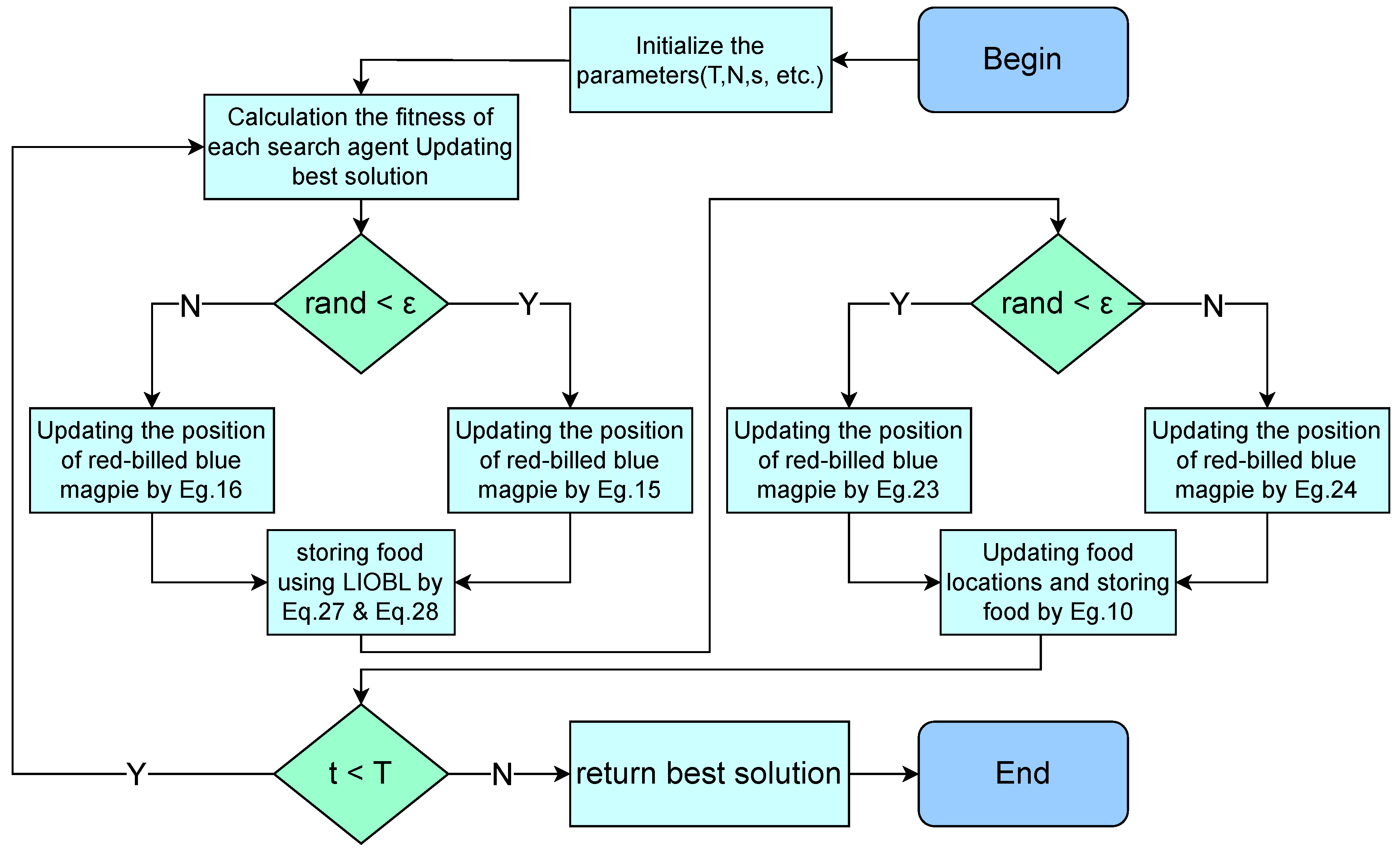
7.6. Worflow of MRBMO

The worflow of MRBMO is provided in Figure 8.

8. Performance Test

The experimental environment for experiments was Windows 11 (64bit), Intel(R) Core(TM) i5-8300H CPU @ 2.30GHz, 8GB running memory and the simulation platform is Matlab R2023a.

In order to validate the performance and effectiveness of MRBMO, the following two experiments are designed to test the algorithms on 23 classical benchmark functions and simulation experiment for engineering design optimization and antenna S-parameter optimization will be performed in next chapter:

• Each of the four improvement strategies is removed from MRBMO and an ablation study is performed on the 23 classical benchmark functions in Table 1;
• A qualitative analysis experiment was performed by applying MRBMO on the benchmark functions to comprehensively evaluate the performance, robustness and exploration-exploitation balance of MRBMO in different types of problems, by assessing convergence behavior, population diversity and exploration-exploitation capability;
• MRBMO, traditional RBMO and other outstanding metaheuristic algorithms are examined on the classical benchmark functions.

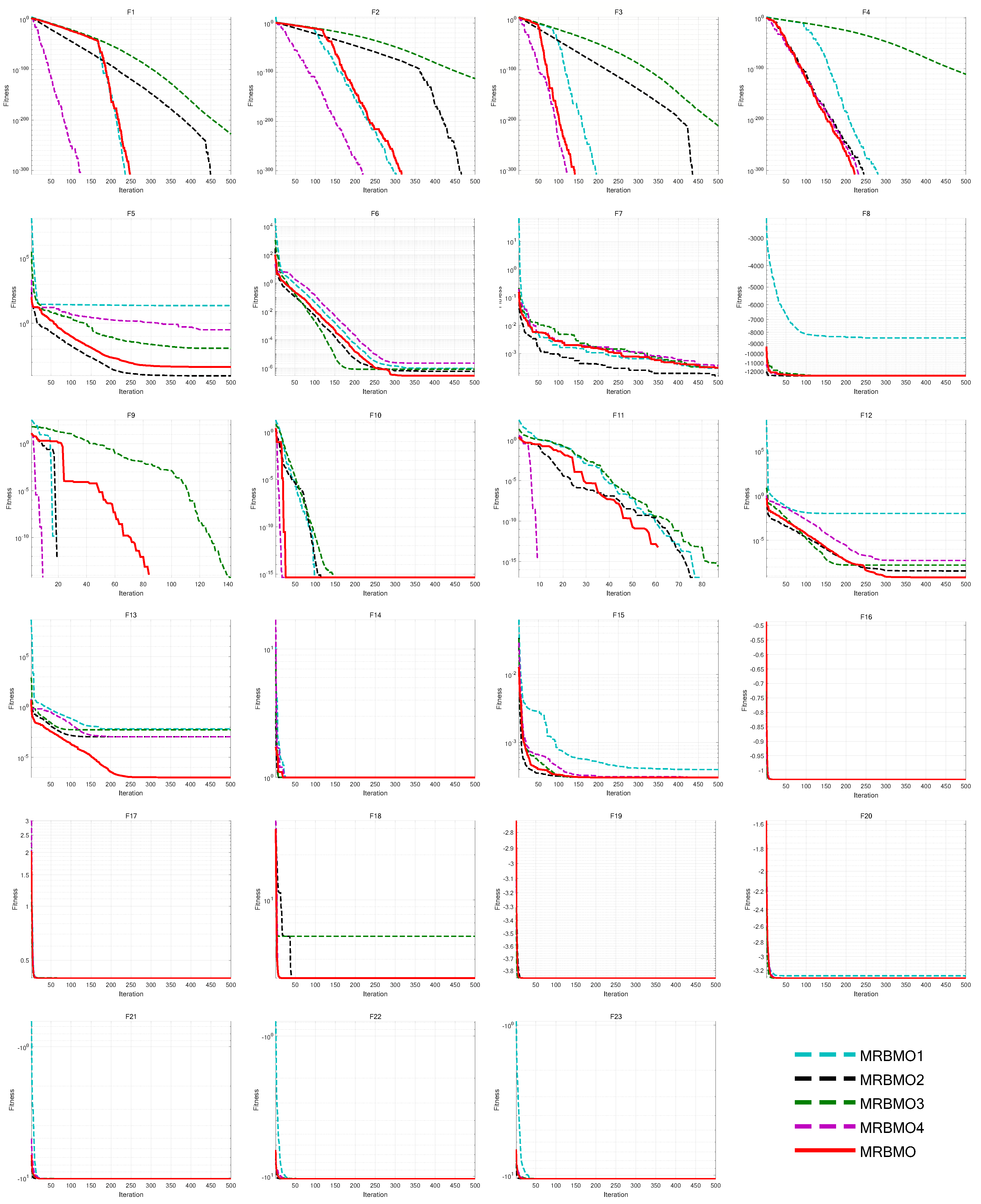
8.1. Ablation Study

This paper designs an ablation study to evaluate the effectiveness of various improvement strategies on RBMO. We define the following variants: MRBMO1 is the MRBMO removes the Good Nodes Set initialization. MRBMO2 is the MRBMO which removes Enhanced Search-for-prey Strategy. MRBMO3 is the MRBMO which removes Siege-style Attacking-prey Strategy. And MRBMO4 is the MRBMO which removes LIOBL. To fairly compare the effectiveness of each strategy, we test these improved algorithms on 23 benchmark functions. We set the maximum iteration as T=500 and the population size as N=30. We run each algorithm on the 23 functions for 30 times and the results are shown in Figure 9.

Experimental results show that each improvement strategy significantly enhances RBMO’s performance. The Good Nodes Set Initialization distributes the population evenly in the solution space, improving quality and aiding in solving high-dimensional multi-modal functions like F5, F8, F12 and F13. As shown in F6, F7 and F13, the Enhanced Search-for-food Strategy sacrifices a slight reduction in convergence speed but improves the optimization ability for handling complex multi-modal functions. As shown in F1-F4 and F9-F13, the Siege-style Attacking-prey Strategy strengthens the exploitation phase, enhancing local search capability and convergence speed. Replacing the Food Storage mechanism with LIOBL allows population updates post-development, increasing diversity while preserving elite individuals, which boosts exploration and reduces local optima entrapment.

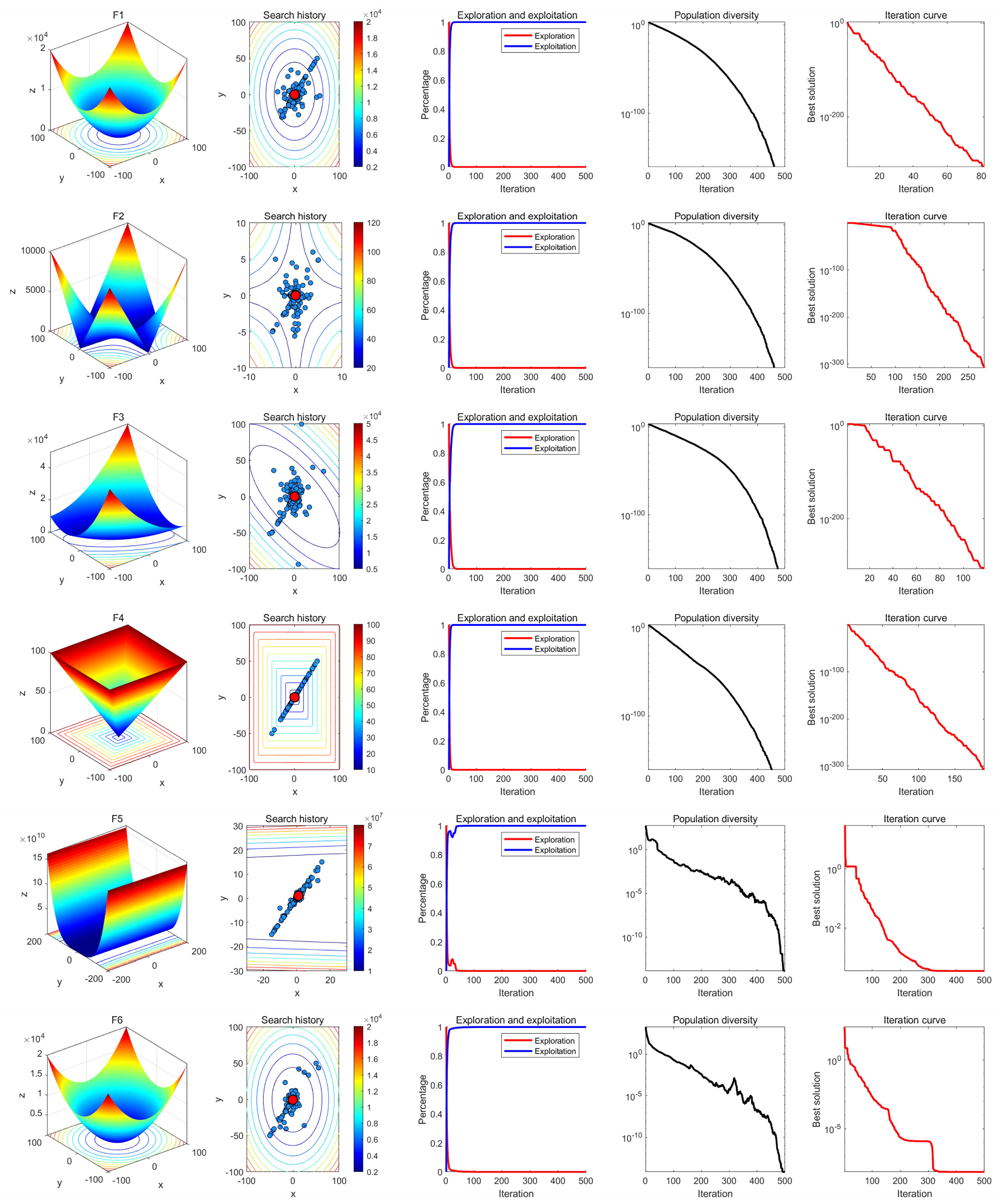
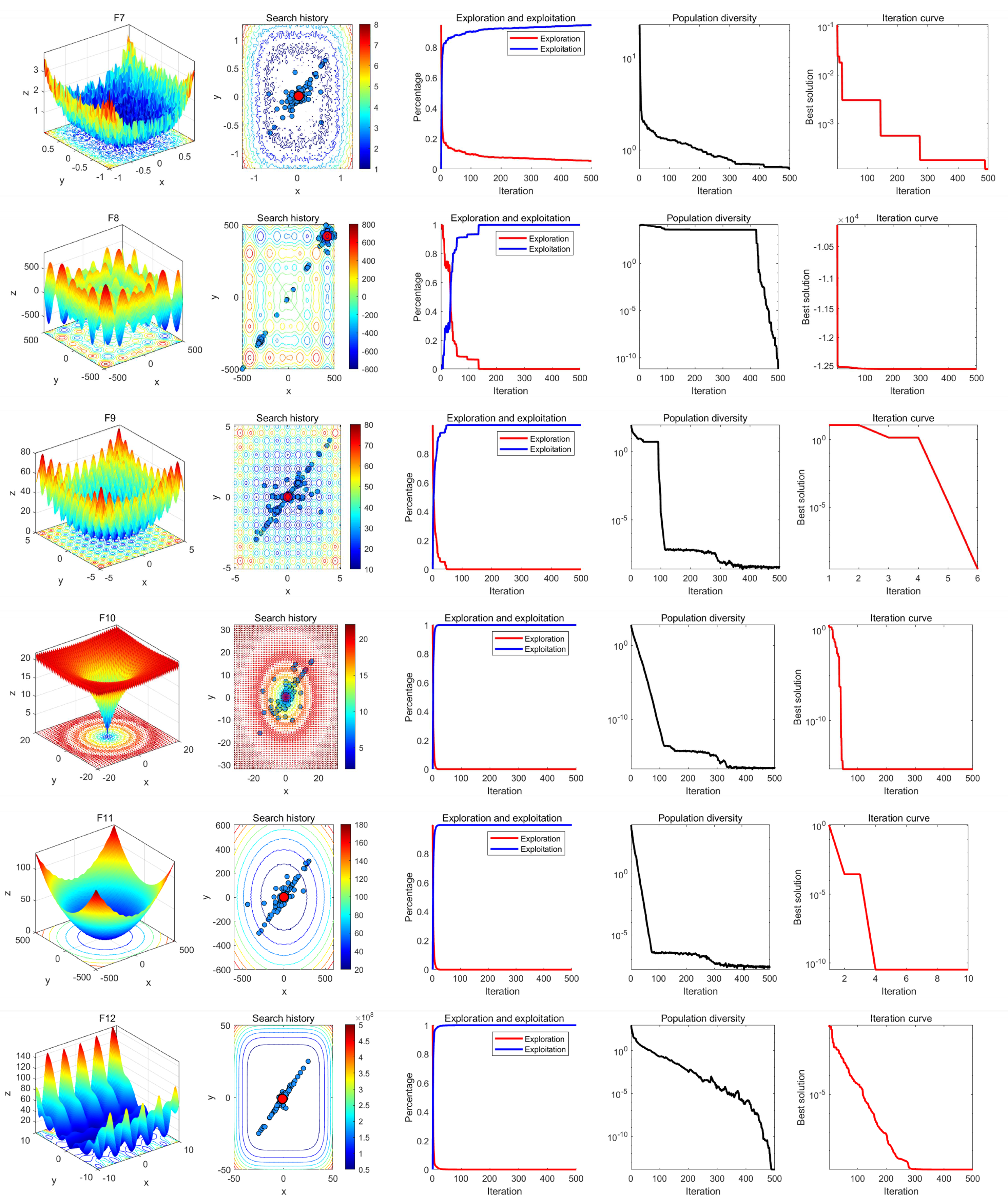
8.2. Qualitative Analysis Experiment

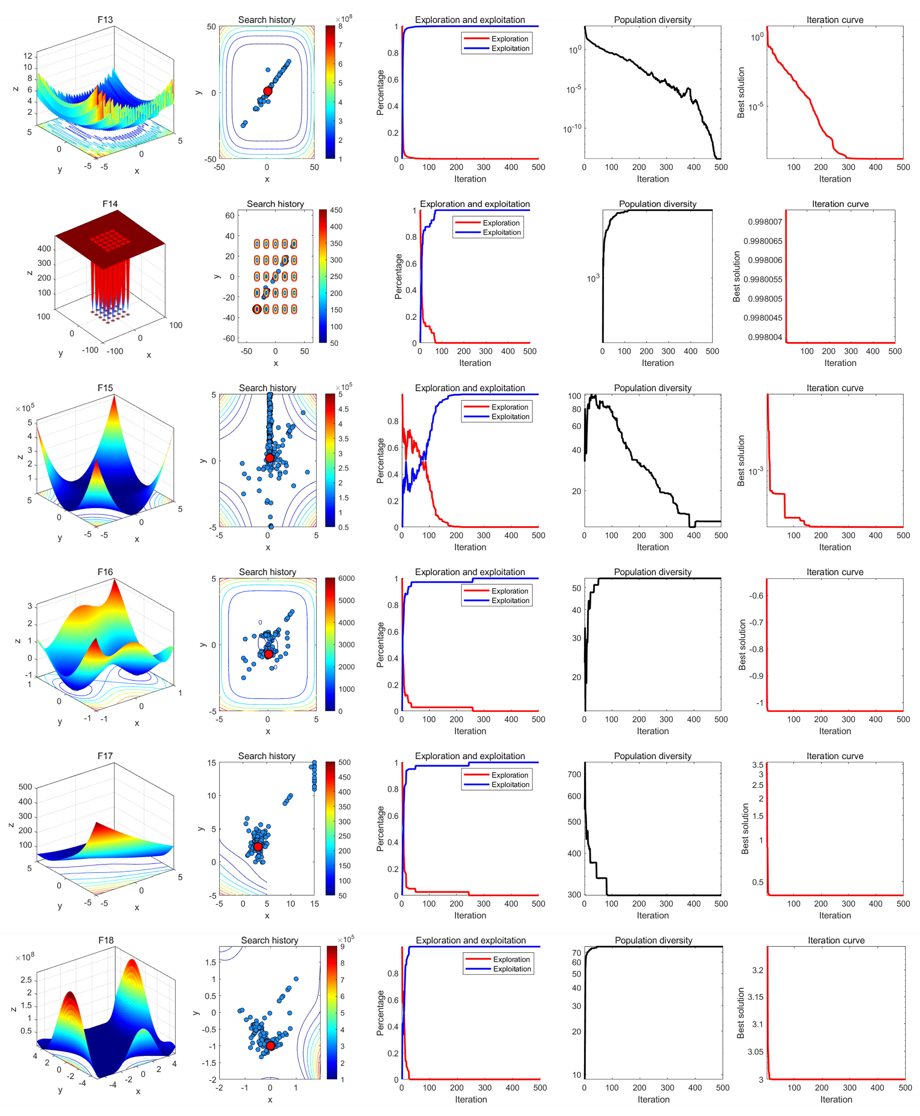
In qualitative analysis experiment, we applied MRBMO on the benchmark functions recorded the search history of the red-billed blue magpie individuals, the exploration-exploitation percentage of MRBMO during the iterations and the polulation diversity of MRBMO. So that we could comprehensively evaluate the performance, robustness and exploration-exploitation balance of MRBMO in different types of problems.

In this experiment, the maximum number of iterations was set to T=500 and the population size was N=30. The search history of the red-billed blue magpie individuals, the proportions of exploration and exploitation, population diversity, and iteration curves were recorded and are presented in Figure 10, Figure 11, Figure 12 and Figure 13. From the figures, it is evident that the red-billed blue magpie individuals in MRBMO demonstrate a well-distributed search within the solution space, indicating the effectiveness of the Good Nodes Set Initialization. For the F8, the global optimal solution is located in the upper-right corner of the solution space, posing significant challenges for the algorithm’s ability to escape local optima. The Siege-style Attacking-prey Strategy facilitates detailed exploration around the region with potential solution, ultimately leading to the identification of the optimal solution for F8. Additionally, the introduction of Levy flight allows MRBMO to consistently escape local optima and maintain high population diversity, even when addressing complex combinatorial problems such as F15-F23. For uni-modal functions, the results show that the exploitation proportion of MRBMO increases rapidly during the iterative process, demonstrating strong exploitation capabilities. For complex functions like F7, F8 and F15, the exploration proportion decreases gradually in the early iterations, reflecting MRBMO’s robust global exploration ability. In the later stages of the iterations, the exploitation proportion increases significantly, indicating strong local exploitation capabilities.

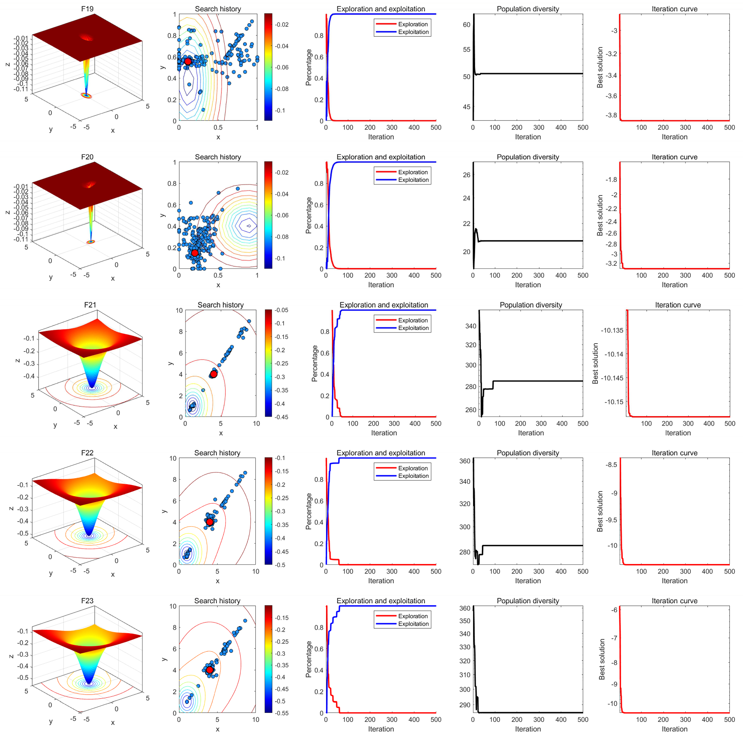
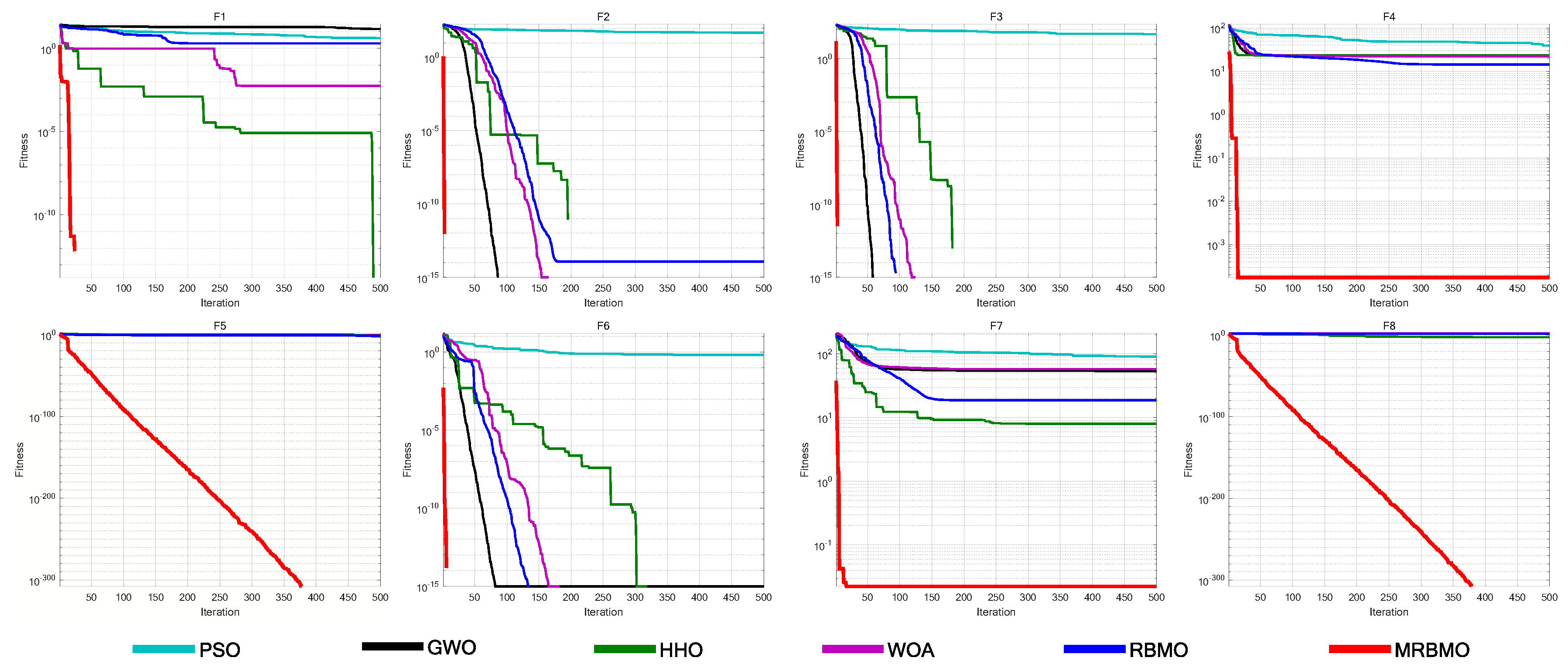
8.3. Superiority Comparative Test

To further verify the superiority of MRBMO, we selected Attraction-Repulsion Optimization Algorithm (AROA) [35], Harris Hawks Optimization (HHO) [7], Grey Wolf Optimizer (GWO) [10], Whale Optimization Algorithm (WOA) [21] and RBMO for superiority comparative experiments. The tests were conducted on 23 benchmark functions. The parameter settings for each algorithm are shown in Table 2. We set population size as N=30, the number of iterations as T=500 and each algorithm is run independently 30 times. And the average fitness (Ave), standard deviation (Std), p-values of Wilcoxon rank-sum test, and Friedman values of 30 runs were recorded for performance analysis. And we will evaluate the overall effectiveness (OE) of MRBMO. The experimental results are presented in Figure 14, Table 3, Table 3 and Table 4.

From the experiment results, it can be seen that MRBMO converges to the optimal value on most functions, with a standard deviation of zero or close to zero, demonstrating strong stability, robustness and optimization capabilities. For problems like F5-F8 and F20-F23, which are prone to local optima, the Good Nodes Set initialization allows population of MRBMO to be evenly distributed in the solution space, significantly improving the population quality. As a result, MRBMO can escape local optima and achieve better solutions for these types of problems. The incorporation of Enhanced Search-for-food Strategy and Siege-style Attacking-prey Atrategy contributes to higher accuracy with solving complex problem like F5-F6 and F12-F13. Siege-style Attacking-prey Strategy helps MRBMO achieve higher convergence speed and accuracy, enabling MRBMO to find the optimal solutions for F1-F4 and F9-F11 within a limited number of iterations.

In non-parametric tests, the statistical results, as is shown in Table 5, indicate that most p-values from Wilcoxon rank-sum tests are less than 0.05, suggesting significant differences between the optimization results of MRBMO and the five comparison algorithms. On F9-F11, there is no significant difference between MRBMO and HHO, because they all found the optimal solutions within a limited number of iterations. There is no significant difference between MRBMO and RBMO on F16, F17, and F19, because MRBMO not only found the optimal solutions for these functions every time but also had a standard deviation equal to or slightly smaller than that of RBMO. This indicates that MRBMO, while maintaining RBMO’s ability to solve complex functions, also achieved faster convergence speed and higher accuracy. And there is a significant difference between MRBMO and the rest algorithms. This experiment further corroborates the reliability of Superiority Test. The average Friedman values for these six algorithms are 5.2985, 3.4449, 3.3703, 3.8087, 3.7580, and 1.3196 respectively. According to these results, MRBMO ranks first in terms of the average Friedman value among the six algorithms, indicating its superior performance. This consistent performance across multiple functions highlights the effectiveness and robustness of MRBMO.

Table 5 summarizes all performance results of MRBMO and other algorithms by a useful metric named overall effectiveness (OE). In Table 5, w indicates win, t indicates tie and l indicates loss. The OE of each algorithm is computed by Eq. 29 [33].

$$OE={\displaystyle \frac{N-L}{L}}·100$$

(29)

where N is the total number of tests; L is the total number of losing tests for each algorithm.

Results proves that MRBMO is competitive with other algorithms on the benchmark functions with different dimensions.

Table 5. Effectiveness of MRBMO and other algorithms

	AROA	HHO	GWO	WOA	RBMO	RBMO
	($\mathit{w}$/$\mathit{t}$/$\mathit{l}$)	($\mathit{w}$/$\mathit{t}$/$\mathit{l}$)	($\mathit{w}$/$\mathit{t}$/$\mathit{l}$)	($\mathit{w}$/$\mathit{t}$/$\mathit{l}$)	($\mathit{w}$/$\mathit{t}$/$\mathit{l}$)	($\mathit{w}$/$\mathit{t}$/$\mathit{l}$)
Total	0/0/23	0/2/21	0/0/23	0/0/23	1/2/20	18/5/1
$OE$	0%	8.69%	0%	0%	13.04%	95.65%

Table 5. Effectiveness of MRBMO and other algorithms

	AROA	HHO	GWO	WOA	RBMO	RBMO
	($\mathit{w}$/$\mathit{t}$/$\mathit{l}$)	($\mathit{w}$/$\mathit{t}$/$\mathit{l}$)	($\mathit{w}$/$\mathit{t}$/$\mathit{l}$)	($\mathit{w}$/$\mathit{t}$/$\mathit{l}$)	($\mathit{w}$/$\mathit{t}$/$\mathit{l}$)	($\mathit{w}$/$\mathit{t}$/$\mathit{l}$)
Total	0/0/23	0/2/21	0/0/23	0/0/23	1/2/20	18/5/1
$OE$	0%	8.69%	0%	0%	13.04%	95.65%

9. Silulation Experiment

To validate the ability of MRBMO to solve real-world problems, we used four engineering design optimzation problems to test the performance of MRBMO, in order to verify the effectiveness and applicability of MRBMO in engineering design optimization. We also used an antenna S-parameter suite to test the performance of MRBMO, in order to quickly validate the effectiveness and applicability of MRBMO in antenna S-parameter optimization.

9.1. Engineering Design Optimzation

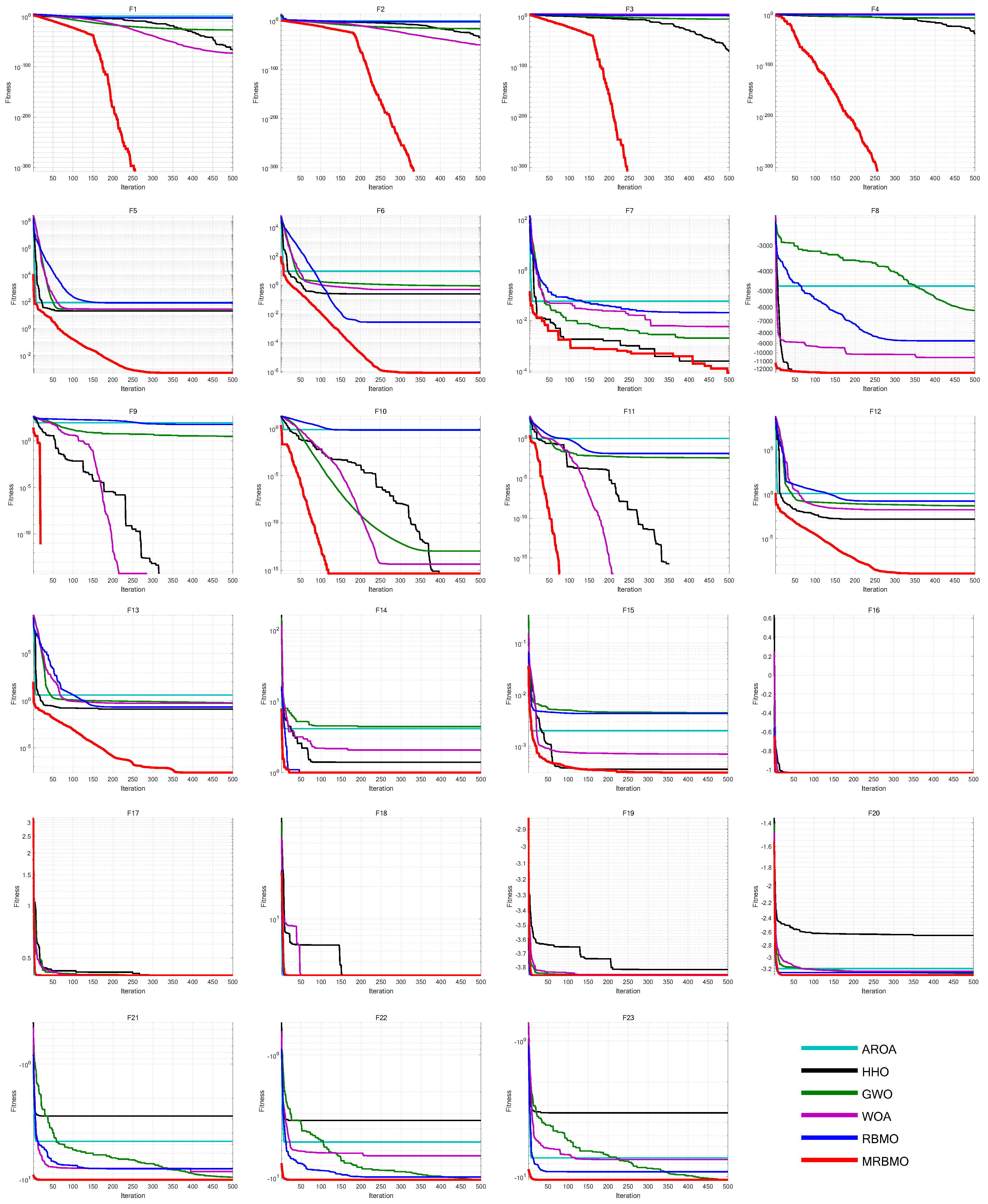
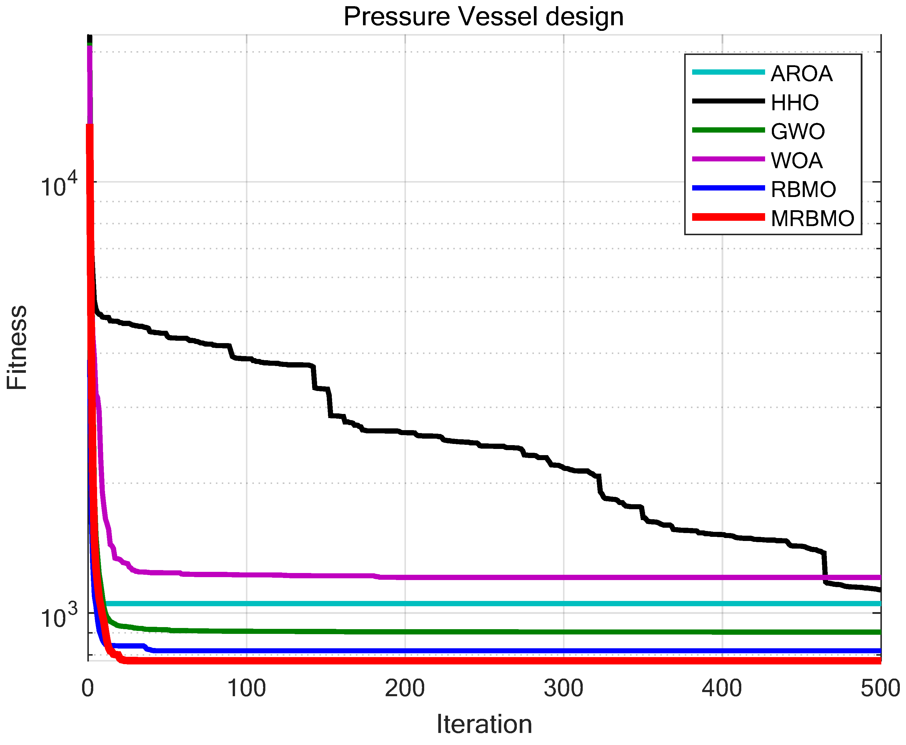
9.1.1. Pressure Vessel Design

A pressure vessel is a common mechanical structure used in fields such as chemical engineering, aerospace, and medical applications. The pressure vessel design problem is a classic structural optimization problem, where the goal is to minimize the manufacturing costs of the pressure vessel, including pairing, forming, and welding processes. The design of the pressure vessel is shown in Figure 15, with caps sealing both ends of the vessel. The cap at one end is hemispherical. $x_1$ and $x_2$ represent the wall thickness of the cylindrical section and the head, respectively, while $x_3$ is the inner diameter of the cylindrical section, and $x_4$ is the length of the cylindrical section, excluding the head. Thus, $x_1$, $x_2$, $x_3$, and $x_4$ are the four optimization variables of the pressure vessel design problem. The objective function and four optimization constraints are represented as follows:

Variable:

$$\begin{array}{cc}\hfill x& =[x_1,x_2,x_3,x_4]\hfill \end{array}$$

Minimize:

$$f\left(x\right)=0.6224x_1·x_3·x_4+1.7781x_2·x_3^2+3.1661x_1^2·x_4+19.84x_1^2·x_3$$

(30)

Subject to:

$$g_1\left(x\right)=-x_1+0.0193x_3\le 0;$$

(31)

$$g_2\left(x\right)=-x_2+0.00954x_3\le 0;$$

(32)

$$g_3\left(x\right)=-\pi x_3^2·x_4-{\displaystyle \frac{4}{3}}\pi x_3^2+1296000\le 0;$$

(33)

$$g_4\left(x\right)=x_4-240\le 0;$$

(34)

Variable range:

$$0\le x_1\le 99;0\le x_2\le 99;10\le x_3\le 200;10\le x_4\le 99;$$

In this study, we conducted comparative tests between the MRBMO and AROA, HHO, GWO, WOA and RBMO. The parameter settings for each algorithm are provided in Table 2. The number of iterations is set to T=500, and the population size is N=30. Each algorithm is run independently for 30 trials on the pressure vessel design problem, and the average values and standard deviations are recorded for performance analysis. The experimental results are shown in Figure 16 and Table 7. As shown in Table 7, MRBMO significantly outperforms the other algorithms in terms of both optimization accuracy and stability for the pressure vessel design problem. This demonstrates that MRBMO has superior solving capabilities when handling this type of problem.

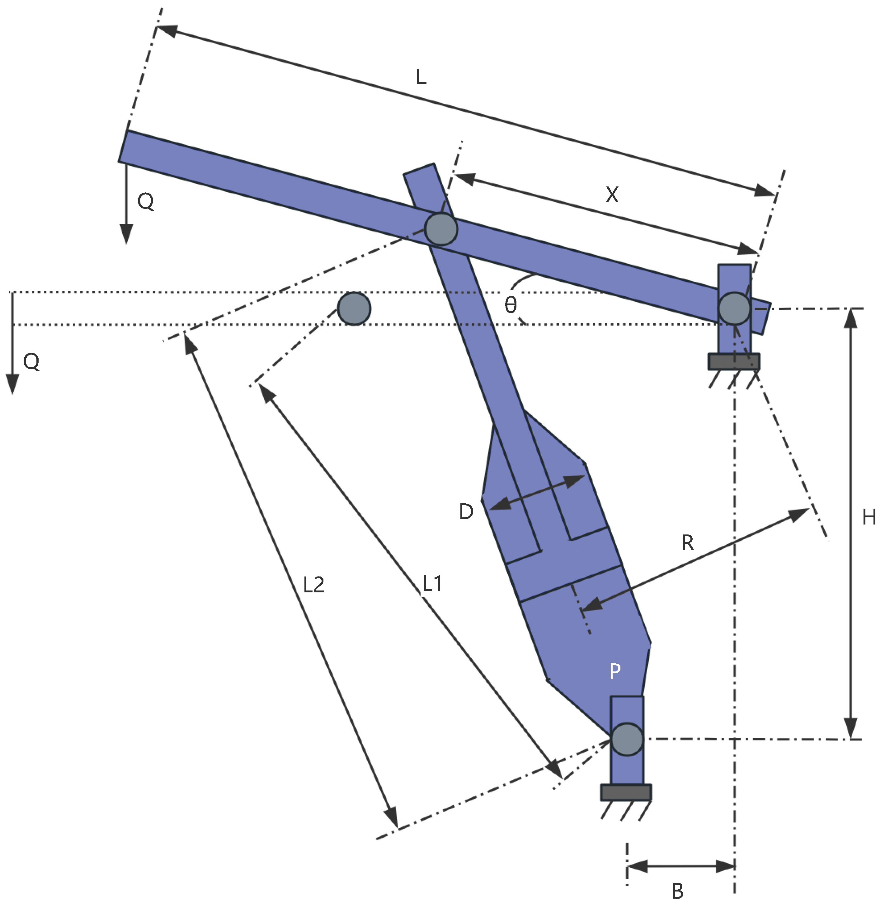
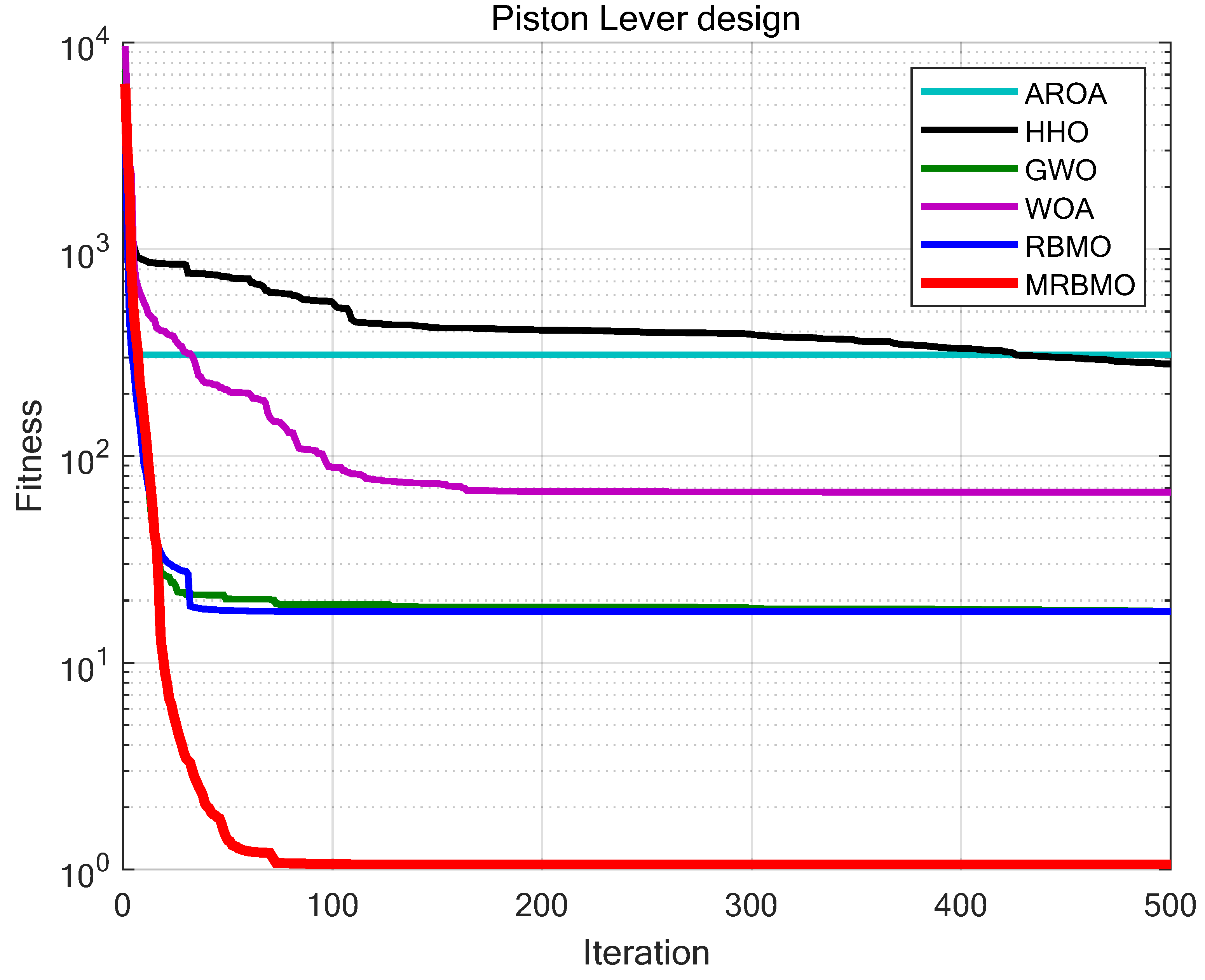
9.1.2. Piston Lever Design

A piston lever is a typical mechanical structure, as shown in Figure 17, and its design problem is classified as a classical engineering optimization problem. It involves the adjustment of multiple geometric and mechanical parameters with the aim of minimizing material usage or structural weight while satisfying constraints such as strength and stability. This optimization seeks to achieve a balance between economic efficiency and structural performance and is widely applied in mechanical engineering, vehicle design, and other industrial scenarios, especially in lightweight and efficient design of moving components.

In the Piston Lever design problem, the objective is to minimize the total material consumption of the Piston Lever while ensuring that the structural strength and performance meet design requirements. The geometric structure of the Piston Lever is defined by multiple design parameters that describe the relationships between its key dimensions. In this problem, the Piston Lever consists of multiple structural parts with the following important characteristics: one end is fixed, while the other end bears an applied force; its mechanical properties are influenced by geometric features such as radius and length; and the design of each geometric part is controlled by decision variables. From the geometric relationships, the meanings of variables $x_1$ to $x_4$ are as follows: $x_1$ and $x_2$ are Primary length and width parameters of the geometric structure, which govern the overall lever arm. $x_3$ is cross-sectional radius at the point of force application, affecting force distribution. $x_4$ is Geometric dimension related to the support point.

The objective function for the Piston Lever design problem can be described as,

Variable:

$$\begin{array}{c}\hfill x=[x_1,x_2,x_3,x_4]\end{array}$$

Minimize:

$$f\left(x\right)=0.25\pi x_3^2(L_2-L_1)$$

(35)

Subject to:

$$g_1\left(x\right)=QLcos\theta -RF\le 0;$$

(36)

$$g_2\left(x\right)=Q(L-x_4)-M_{max}\le 0;$$

(37)

$$g_3\left(x\right)=1.2(L_2-L_1)-L_1\le 0;$$

(38)

$$g_4\left(x\right)={\displaystyle \frac{x_3}{2}}-x_2\le 0;$$

(39)

Variable range:

$$\begin{array}{c}\hfill 0.05\le x_1\le 500;0.05\le x_2\le 500;0.05\le x_4\le 500;0.05\le x_3\le 120;\end{array}$$

Where:

$$\begin{array}{c}\hfill Q=10000;P=1500;L=240;M_{max}=1.8\times {10}^6;\end{array}$$

$$\begin{array}{c}\hfill L_1=\sqrt{{(x_4-x_2)}^2+x_1^2};L_2=\sqrt{{(x_{4}sin\theta +x_1)}^2+{(x_2-x_{4}cos\theta )}^2};\end{array}$$

$$\begin{array}{c}\hfill R={\displaystyle \frac{|-x_4(x_{4}sin\theta +x_1)+x_1(x_2-x_{4}cos\theta )|}{\sqrt{{(x_4-x_2)}^2+x_1^2}}};\end{array}$$

$$\begin{array}{c}\hfill F=0.25\pi P{x}_3^2;\end{array}$$

This study compares MRBMO with AROA, HHO, GWO, WOA and RBMO, with the parameter settings for each algorithm shown in Table 2. The number of iterations is uniformly set to T=500, and the population size is set to N=30. Each algorithm is run independently 30 times on the Piston Lever design problem, with the average fitness and standard deviation recorded for performance analysis. The experimental results are shown in Figure 18 and Table 7. As shown in Table 7, in the Piston Lever design problem, MRBMO demonstrates significantly superior optimization accuracy and stability compared to other algorithms. This indicates that MRBMO has a substantial advantage in handling such problems.

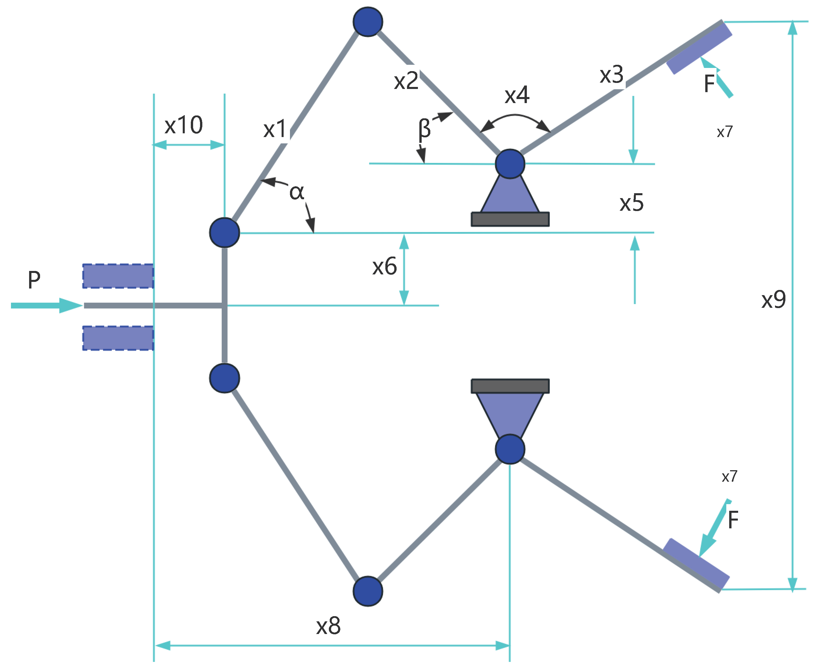
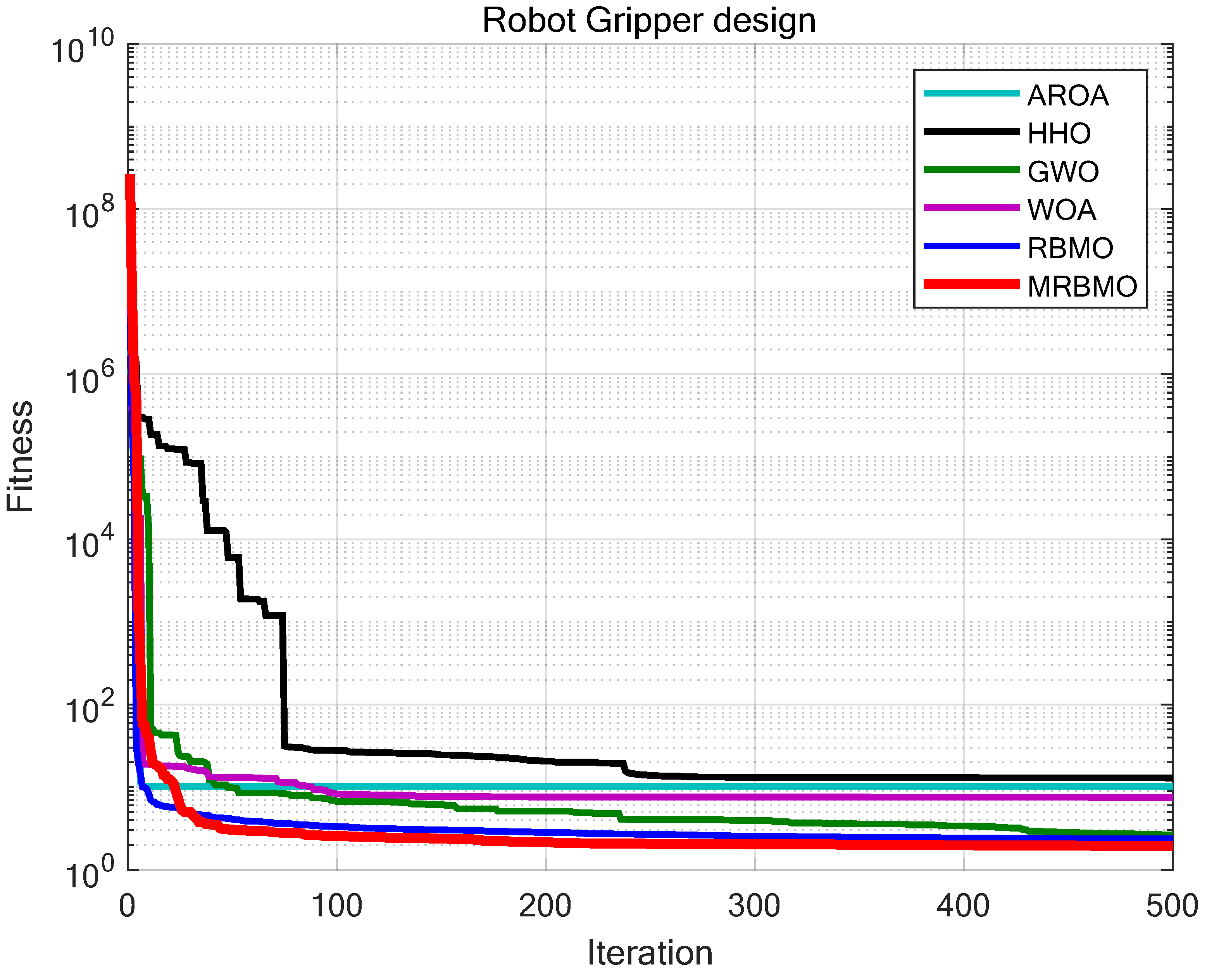
9.1.3. Robot Gripper Design

The robot gripper design problem is a classic engineering optimization problem, widely applied in industrial automation, medical robotics, and logistics. The goal is to maximize gripping performance or minimize material usage under the constraints of gripping force range, structural requirements, and geometric stability, thereby optimizing the structural efficiency and cost-effectiveness of the robot gripper. Figure 19 is the structure of a robot gripper.

The robot gripper involves several critical parameters related to geometry, mechanics, and motion: $x_1$, $x_2$, $x_3$, $x_4$ are geometric parameters of the gripper; $x_5$ is the force applied to the gripper; $x_6$ is the length of the gripper; $x_7$ is the angular offset of the gripper.

The objective function of the Robot Gripper design problem can be described as:

Variable:

$$x=[x_1,x_2,x_3,x_4,x_5,x_6,x_7]$$

(40)

Minimize:

$$f\left(x\right)=-\left[\underset{z\in [0,Z_{max}]}{max}{F}_1(x,z,2)+\underset{z\in [0,Z_{max}]}{min}{F}_1(x,z,2)\right]$$

(41)

Subject to:

$$g_1\left(x\right)=-Y_{min}+F_1(x,Z_{max},1)\le 0;$$

(42)

$$g_2=-F_1(x,Z_{max},1)\le 0;$$

(43)

$$g_3\left(x\right)=Y_{max}-F_1(x,0,1)\le 0;$$

(44)

$$g_4\left(x\right)=F_1(x,0,1)-Y_G\le 0;$$

(45)

$$g_5\left(x\right)=x_6^2+x_4^2-{(x_1+x_2)}^2\le 0;$$

(46)

$$g_6\left(x\right)=x_2^2-{(x_1-x_4)}^2-{(x_6-Z_{max})}^2\le 0;$$

(47)

$$g_7\left(x\right)=Z_{max}-x_6\le 0$$

(48)

Variable range:

$$\begin{array}{c}\hfill 10\le x_1\le 150;10\le x_2\le 150;100\le x_3\le 200;0\le x_4\le 50;\end{array}$$

$$\begin{array}{c}\hfill 10\le x_5\le 150;100\le x_6\le 300;1\le x_7\le 3.14\end{array}$$

Where:

$$\begin{array}{c}\hfill P=100;Z_{max}=100;\end{array}$$

$$\begin{array}{c}\hfill Y_{min}=50;Y_{max}=100;Y_G=150;\end{array}$$

$$\begin{array}{c}\hfill F_1(x,z,flag):\mathrm{Calculate}\mathrm{the}\mathrm{grabbing}\mathrm{force}\mathrm{or}\mathrm{the}\mathrm{applied}\mathrm{force}\end{array}$$

$$\begin{array}{c}\hfill \mathrm{When}\mathrm{Flag}=1,\mathrm{calculate}\mathrm{the}\mathrm{grabbing}\mathrm{force}:\end{array}$$

$$\begin{array}{c}\hfill F_1(x,z,1)=2\left(x_5+x_4+x_3·sin(\beta +x_7)\right);\end{array}$$

When Flag=2, calculate the applied force:

$$\begin{array}{c}\hfill F_1(x,z,2)={\displaystyle \frac{P{x}_2·sin(\alpha +\beta )}{2x_3}};\end{array}$$

$$\begin{array}{c}\hfill \alpha =arccos\left({\displaystyle \frac{x_1^2+g^2-x_2^2}{2x_{1}g}}\right)+{\varphi }_o;\end{array}$$

$$\begin{array}{c}\hfill \beta =arccos\left({\displaystyle \frac{x_2^2+g^2-x_1^2}{2x_{2}g}}\right)-{\varphi }_o;\end{array}$$

$$\begin{array}{c}\hfill g=\sqrt{x_4^2+{(z-x_6)}^2};\end{array}$$

$$\begin{array}{c}\hfill {\varphi }_o=arctan\left({\displaystyle \frac{x_4}{x_6-z}}\right)\end{array}$$

This study compares MRBMO with AROA, HHO, GWO, WOA, and RBMO. The parameter settings for each algorithm are shown in Table 2. The iteration number T=500 and population size N=30 were uniformly set for all experiments. Each algorithm was executed independently 30 times on the robot gripper design problem, and the average fitness value and standard deviation were recorded for performance analysis. The experimental results are presented in Figure 20 and Table 6.

From Table 6, it can be observed that in the Robot Gripper design problem, MRBMO significantly outperforms other algorithms in terms of optimization accuracy and stability. This demonstrates that MRBMO has a considerable advantage in addressing such problems..

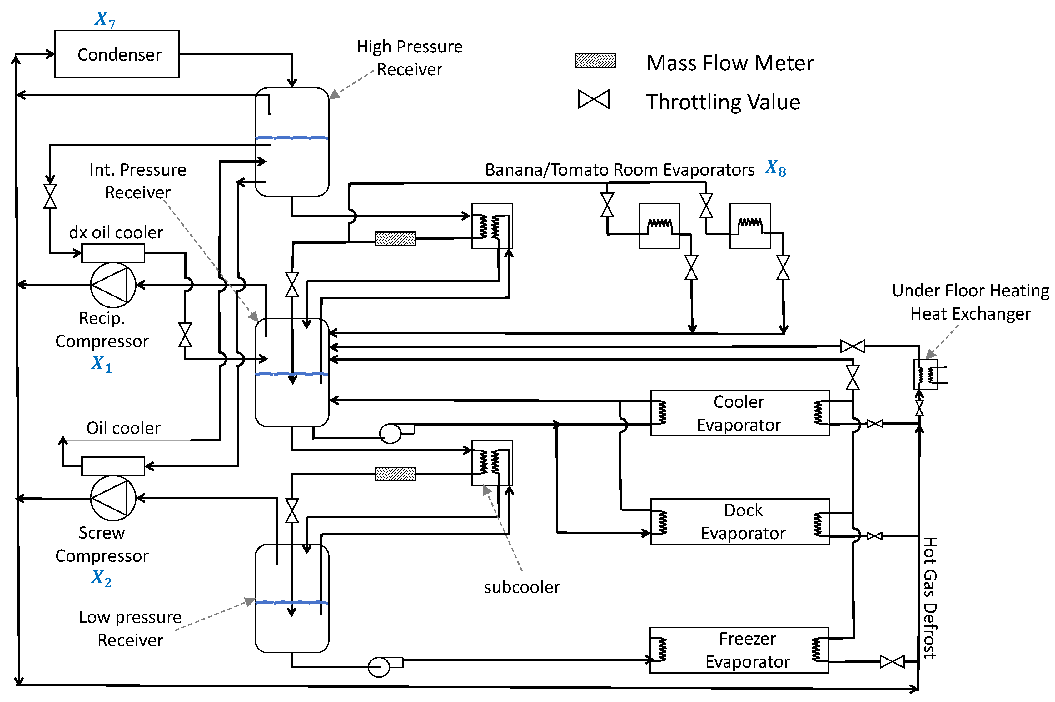
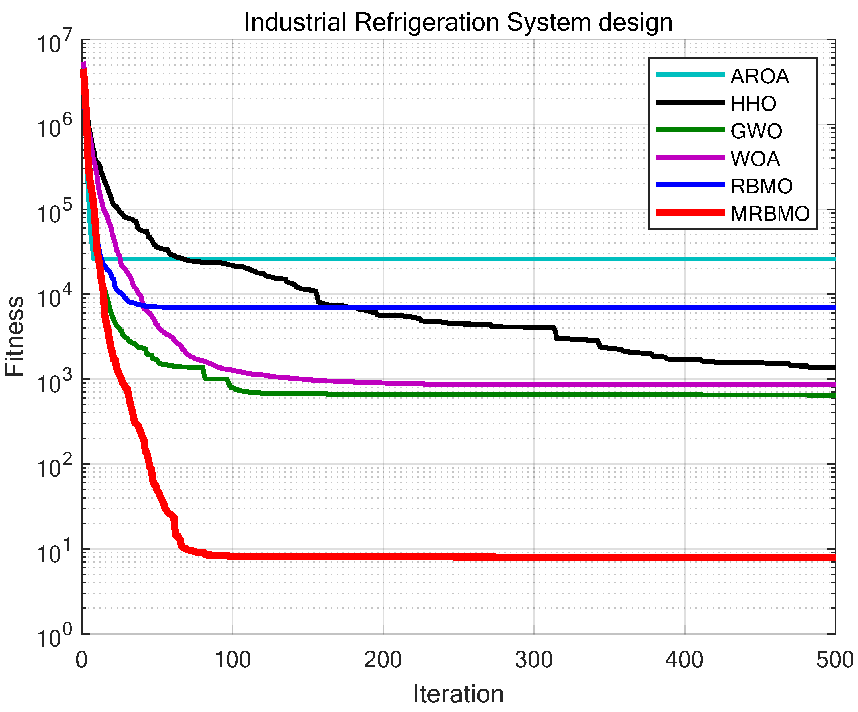
9.2. Industrial Refrigeration System Design

In the chemical plant design, an industrial refrigeration system is one of the key auxiliary facilities, widely used in chemical production processes, especially in operations such as chemical reactions, storage, transportation, and refining, where temperature control and heat exchange are critical. Chemical plants often require significant cooling and temperature control to maintain reaction stability, ensure product quality, reduce energy consumption and emissions, and ensure the proper functioning of equipment. Therefore, industrial refrigeration systems play a crucial role in the design of chemical plants. The industrial refrigeration system design problem focuses on minimizing energy consumption and cost while ensuring efficient cooling performance, as shown in Figure 21. The objective is to configure the system components, such as compressors, condensers, and evaporators, to achieve the lowest operating cost and optimal heat exchange efficiency. The problem includes fourteen variables: compressor power $x_1$ and $x_2$, refrigerant flow rate and mass flow $x_3$ through $x_6$, characteristics of the condenser and evaporator $x_7$ and $x_8$, compression ratios $x_9$ and $x_{10}$, temperature parameters $x_{11}$ and $x_{12}$, and flow rate parameters $x_{13}$ and $x_{14}$. Specifically, compressor power $x_1$ and $x_2$ control the cooling capacity; refrigerant flow rate and mass flow $x_3$ through $x_6$ indicate the refrigerant flow through condensers, evaporators, and receivers; $x_7$ and $x_8$ represent the sizing parameters of the condenser and evaporator; $x_9$ and $x_{10}$ define the compression degree and compressor efficiency; $x_{11}$ and $x_{12}$ manage the temperature differential for heat exchange; and $x_{13}$ and $x_{14}$ govern the flow rate of cooling water or refrigerant, affecting overall system performance. Industrial refrigeration system design problem is modeled below.

Variable:

$$\begin{array}{cc}\hfill x& =[x_1,x_2,x_3,x_4,x_5,x_6,x_7,x_8,x_9,x_{10},x_{11},x_{12},x_{13},x_{14}]\hfill \end{array}$$

Minimize:

$$y=f\left(x\right)$$

(49)

Subject to:

$$g_1={\displaystyle \frac{1.524}{x_7}}-1\le 0;$$

(50)

$$g_2={\displaystyle \frac{1.524}{x_8}}-1\le 0;$$

(51)

$$g_3=0.07789·x_1-{\displaystyle \frac{2·x_9}{x_7}}-1\le 0;$$

(52)

$$g_4={\displaystyle \frac{7.05305·x_1^2·x_{10}}{x_9·x_8·x_2·x_{14}}}-1\le 0;$$

(53)

$$g_5={\displaystyle \frac{0.0833·x_{14}}{x_{13}}}-1\le 0;$$

(54)

$$g_6={\displaystyle \frac{47.136·x_2^{0.333}·x_{12}}{x_{10}}}-1.333·x_8·x_{13}^{2.1195}+{\displaystyle \frac{62.08·x_{13}^{2.1195}·x_8^{0.2}}{x_{12}·x_{10}}}-1\le 0;$$

(55)

$$g_7=0.04771·x_{10}·x_8^{1.8812}·x_{12}^{0.3424}-1\le 0;$$

(56)

$$g_8=0.0488·x_9·x_7^{1.893}·x_{11}^{0.316}-1\le 0;$$

(57)

$$g_9={\displaystyle \frac{0.0099·x_1}{x_3}}-1\le 0;$$

(58)

$$g_{10}={\displaystyle \frac{0.0193·x_2}{x_4}}-1\le 0;$$

(59)

$$g_{11}={\displaystyle \frac{0.0298·x_1}{x_5}}-1\le 0;$$

(60)

$$g_{12}={\displaystyle \frac{0.056·x_2}{x_6}}-1\le 0;$$

(61)

$$g_{13}={\displaystyle \frac{2}{x_9}}-1\le 0;$$

(62)

$$g_{14}={\displaystyle \frac{2}{x_{10}}}-1\le 0;$$

(63)

$$g_{15}={\displaystyle \frac{x_{12}}{x_{11}}}-1\le 0;$$

(64)

Where:

$$f\left(x\right)=63098.88·x_2·x_4·x_{12}+5441.5·x_2^2·x_{12}+115055.5·x_2^{1.664}·x_6$$

$$+6172.27·x_2^2·x_6+63098.88·x_1·x_3·x_{11}+5441.5·x_1^2·x_{11}$$

$$+115055.5·x_1^{1.664}·x_5+6172.27·x_1^2·x_5+140.53·x_1·x_{11}$$

$$+281.29·x_3·x_{11}+70.26·x_1^2+281.29·x_1·x_3+281.29·x_3^2$$

$$+14437·x_8^{1.8812}·x_{12}^{0.3424}·x_{10}·x_1^2·{\displaystyle \frac{x_7}{x_{14}·x_9}}$$

$$+20470.2·x_7^{2.893}·x_{11}^{0.316}·x_{12}$$

Variable range:

$$0.001<x_1<5;0.001<x_2<5;0.001<x_3<5;0.001<x_4<5;$$

$$0.001<x_5<5;0.001<x_6<5;0.001<x_7<5;0.001<x_8<5;$$

$$0.001<x_9<5;0.001<x_{10}<5;0.001<x_{11}<5;0.001<x_{12}<5;$$

$$0.001<x_{13}<5;0.001<x_{14}<5;$$

A comparative test was also conducted between MRBMO and AROA, HHO, GWO, WOA, and RBMO, with parameters as specified in Table 2. Each algorithm ran independently for 30 trials, maintaining a maximum iterations of T=500 and a population size of N=30. The experimental results, presented in Figure 22 and Table 6. The results demonstrate that MRBMO consistently escapes local optima, continuously searching for better solutions even when other algorithms are trapped in sub-optimal states. Compared with other algorithms, MRBMO shows exceptional stability and accuracy in solution-seeking. Therefore, MRBMO proves to be a highly robust and outstanding optimization tool for handling complex design optimization tasks.

Table 6. Results of different algorithms on various engineering design optimization problems

Problems	Index	AROA	HHO	GWO	WOA	RBMO	MRBMO
Pressure vessel	Ave	1051.497457	1131.127862	903.228152	1209.015966	817.427522	774.810116
	Std	284.348170	279.641639	275.992023	547.039872	195.056827	96.712573
Piston lever	Ave	237.669131	374.504869	51.098610	41.949668	17.698731	1.057175
	Std	165.924633	203.438416	80.569535	83.949697	52.625219	0.000000
Robot gripper	Ave	10.245274	12.850251	2.634413	7.488088	2.360270	1.940320
	Std	10.434973	23.741498	1.835745	18.086681	0.833777	0.549999
Industrial refrigeration	Ave	25855.679209	1351.066268	646.177525	861.821754	6987.501406	7.900666
system	Std	19798.951282	4597.977707	3496.391366	4161.740403	9330.060337	0.814027

Table 6. Results of different algorithms on various engineering design optimization problems

Problems	Index	AROA	HHO	GWO	WOA	RBMO	MRBMO
Pressure vessel	Ave	1051.497457	1131.127862	903.228152	1209.015966	817.427522	774.810116
	Std	284.348170	279.641639	275.992023	547.039872	195.056827	96.712573
Piston lever	Ave	237.669131	374.504869	51.098610	41.949668	17.698731	1.057175
	Std	165.924633	203.438416	80.569535	83.949697	52.625219	0.000000
Robot gripper	Ave	10.245274	12.850251	2.634413	7.488088	2.360270	1.940320
	Std	10.434973	23.741498	1.835745	18.086681	0.833777	0.549999
Industrial refrigeration	Ave	25855.679209	1351.066268	646.177525	861.821754	6987.501406	7.900666
system	Std	19798.951282	4597.977707	3496.391366	4161.740403	9330.060337	0.814027

9.3. Antenna S-Parameter Optimization

The optimization of antenna S-parameters (scattering parameters) is a critical aspect of the design of wireless communication systems, radar, and other electronic devices, serving as a key factor in ensuring the efficient operation of wireless systems. S-parameters describe the reflection and transmission characteristics of antennas, primarily including $S_{11}$ (reflection coefficient) and $S_{21}$ (transmission coefficient). Optimizing these parameters can enhance antenna performance, reduce signal loss, and improve radiation efficiency. metaheuristic algorithms are capable of finding optimal or near-optimal solutions within complex design spaces. When integrated with electromagnetic simulation software, they create an iterative optimization workflow. Designers can effectively optimize the S-parameters of antennas, thereby enhancing their performance and reliability, by selecting appropriate algorithms, configuring suitable parameters, and utilizing relevant objective functions. However, validating the suitability of algorithms for optimizing antenna S-parameters through simulation can be time-consuming and resource-intensive.Therefore, Zhen Zhang et al. 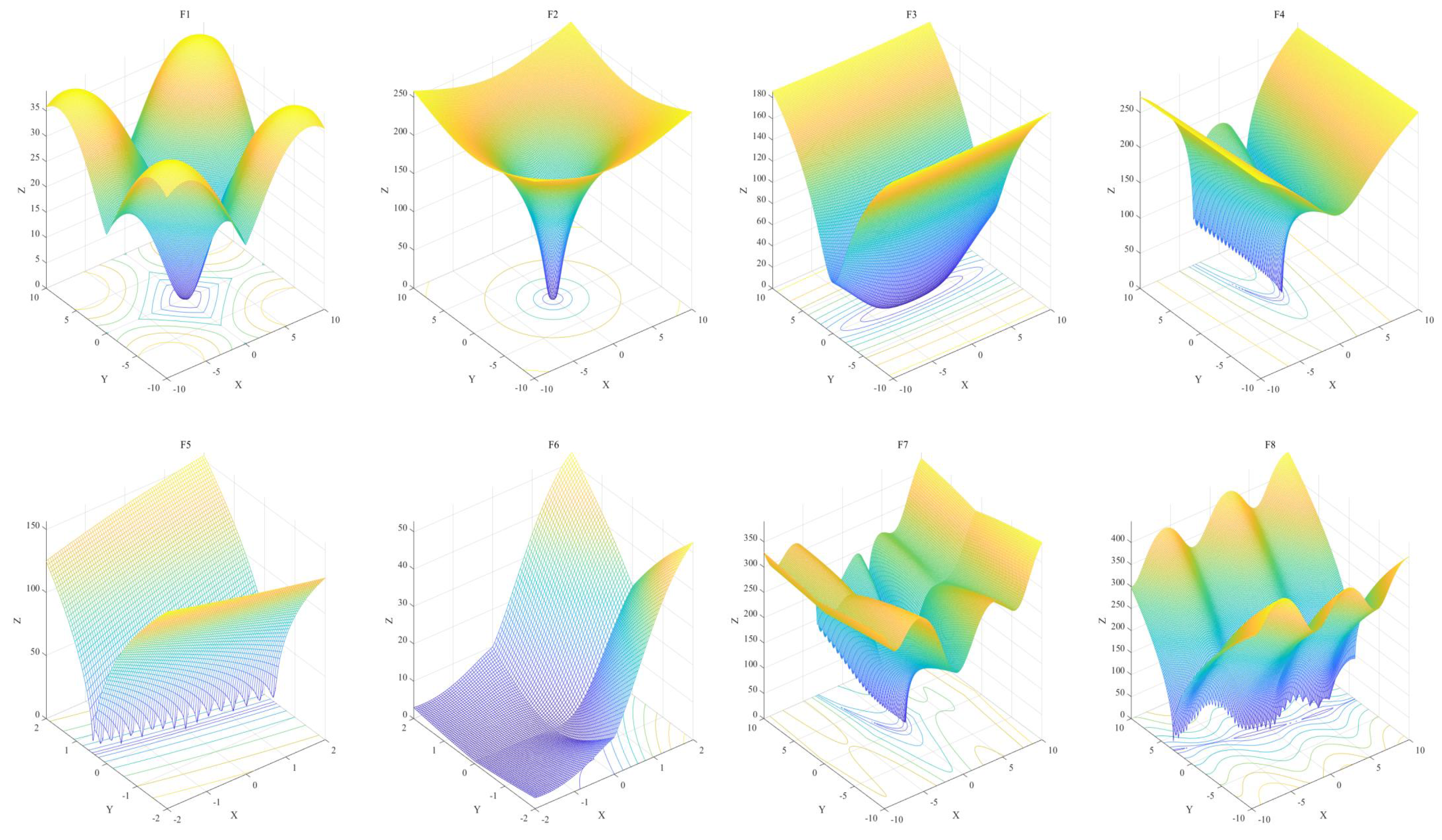developed a benchmark test suite for antenna S-parameter optimization [11] to intuitively and rapidly assess the performance of metaheuristic algorithms in antenna design. This benchmark suite simulates the characteristics of electromagnetic simulations and addresses common antenna issues, ranging from single antennas to multiple antennas, thereby tackling the structural design challenges for both types. They demonstrated that the test suite they proposed has the same effect as the electromagnetic simulation of antenna S-parameters, that is, if an algorithm performs well on the test suite, it is suitable for antenna S-parameter optimization. Details of the benchmark functions of the test suite is listed below and Figure 23 is the landscapes of the functions.

$$F1=20log\left(2\right(\sum _{i=1}^n|sin{\left({\displaystyle \frac{x_i}{8}}\right)}^2|+\sum _{i=1}^n|sin\left({\displaystyle \frac{x_i}{8}}\right)\left|\right)+1)$$

(65)

where $F1$ is a uni-modal function characterized by a rose-shaped valley, with a minimum value of 0 and a dimension of 8. It is continuous, differentiable, and non-separable for single antenna optimization.

$$F2=20log(10{\left(\sum _{i=1}^n{x}_i^2\right)}^2+1)$$

(66)

where $F2$ is a uni-modal function with a steep narrow valley, having a minimum value of 0 and a dimension of 8. It is continuous, differentiable, separable, and scalable, for multi-antenna design optimization.

$$F3=20log(10{\left(\sum _{i=1}^{n}0.01i^5{x}_i^2\right)}^2+1)$$

(67)

where $F3$ is a uni-modal function featuring a long narrow valley, with a minimum value of 0 and a dimension of 8. It is continuous, differentiable, separable, and scalable, for both single and multiple antenna optimization.

$$F4=20log(\left(\sum _{i=1}^n(100{(x_{i+1}-x_i^2)}^2-{(x_i-1)}^2)\right)+1)$$

(68)

where $F4$ is a uni-modal function characterized by steep and banana-shaped curved valleys, with a minimum value of 0 and a dimension of 8. It is continuous, differentiable, non-separable, and scalable, for multi-antenna design optimization.

$$F5=100\sqrt{|x_2+1-0.01{(x_1-10)}^2|}+0.01\left|x_1\right|$$

(69)

where $F5$ is a multi-modal function with long narrow valleys, having a minimum value of 0 and a dimension of 2. It is continuous, non-differentiable, non-separable, and non-scalable, for multi-antenna design optimization.

$$F6=20log\left(\right(0.01(\sum _{i=1}^n|x_i{\left|\right)}^2{(sin\left(0.8x_1\right)+2)}^2+1)$$

(70)

where $F6$ is a multi-modal function with long narrow valleys that intersect, featuring a minimum value of 0 and a dimension of 8. It is continuous, scalable, non-differentiable, and non-separable, for multi-antenna optimization.

$$\begin{array}{c}\hfill F7=20log\left((\sum _{i=1}^{n-1}{\left(100(x_{i+1}-x_i^2)\right)}^2-{(x_i-1)}^2)\right)+1)\\ \hfill +20log\left(0.01\right(\sum _{i=1}^n|x_i{\left|\right)}^2{(sin\left(0.8x_1\right)+2)}^2+1)\end{array}$$

(71)

where $F7$ is a multi-modal compositional function with long narrow and intersecting valleys, with a minimum value of 0 and a dimension of 8. It is continuous, non-differentiable, non-separable, and scalable, for multi-antenna design optimization.

$$\begin{array}{c}\hfill F8=100\sqrt{|x_2+1-0.01{(x_1-10)}^2|}+0.01\left|x_1\right|\\ \hfill +20log\left(0.01\right(\sum _{i=1}^n|x_i{\left|\right)}^2{(sin\left(0.8x_1\right)+2)}^2+1)\end{array}$$

(72)

where $F8$ is a multi-modal function characterized by long narrow and intersecting valleys, with a minimum value of 0 and a dimension of 8. It is continuous, non-differentiable, non-separable, and scalable, for multi-antenna optimization.

We selected AROA, HHO, GWO, WOA, RBMO, and MRBMO to evaluate their performance on the antenna S-parameter optimization through the benchmark test suite. Both the number of iterations T=500 and the population size N=30 were kept consistent across all tests. Each algorithm was executed independently for 30 runs on eight benchmark functions from the suite, and we recorded average fitness, standard deviation, p-value from the Wilcoxon rank-sum test, and Friedman value for comprehensive performance analysis.Based on the experimental results, MRBMO excels in the antenna S-parameter optimization benchmark suite, significantly outperforming the other algorithms. MRBMO exhibits rapid convergence speeds and high accuracy across many functions. In particular, MRBMO showcases robust optimization capabilities in the benchmark functions. Additionally, the Wilcoxon rank-sum test and Friedman test confirm that MRBMO’s performance in various aspects is significantly superior to that of the other algorithms, highlighting its overall excellence.

Table 7. Comparative results of each algorithm in antenna S-parameter optimization

Functions	Index	AROA	HHO	GWO	WOA	RBMO	MRBMO
F1	Ave	1.7007E+00	9.2124E-08	8.6647E-01	1.4631E-02	5.2133E-01	0.0000E+00
	Std	1.5126E+00	4.6530E-07	1.2638E+00	3.5044E-02	5.5072E-02	0.0000E+00
F2	Ave	4.2205E-02	0.0000E+00	0.0000E+00	0.0000E+00	0.0000E+00	0.0000E+00
	Std	1.2381E-01	0.0000E+00	0.0000E+00	0.0000E+00	0.0000E+00	0.0000E+00
F3	Ave	3.6173E+00	0.0000E+00	0.0000E+00	0.0000E+00	0.0000E+00	0.0000E+00
	Std	6.4519E+00	0.0000E+00	0.0000E+00	0.0000E+00	0.0000E+00	0.0000E+00
F4	Ave	1.8043E+01	9.0489E+00	1.4741E+01	1.5110E+01	4.1788E+00	1.0350E-12
	Std	2.1884E-01	9.0112E+00	1.1248E+00	3.2140E+00	6.2593E+00	3.6532E-12
F5	Ave	1.1390E-01	3.9068E-02	1.1857E-01	3.2537E-02	2.1036E-02	0.0000E+00
	Std	1.0944E-01	8.1350E-02	9.1713E-02	1.5953E-02	1.5856E-02	0.0000E+00
F6	Ave	1.6116E-02	0.0000E+00	0.0000E+00	0.0000E+00	0.0000E+00	0.0000E+00
	Std	3.2889E-02	0.0000E+00	0.0000E+00	0.0000E+00	0.0000E+00	0.0000E+00
F7	Ave	3.8973E+01	1.1164E+01	2.4949E+01	2.5166E+01	1.4856E+01	8.5536E-07
	Std	3.0862E+00	1.6702E+01	3.9713E+00	8.1446E+00	2.4862E-05	4.3045E-06
F8	Ave	3.6929E+01	0.0026409	1.6150E+01	50.6156	2.7344E+01	0.0000E+00
	Std	1.5096E+01	6.6231E-03	1.6858E+01	1.9452E+01	1.6428E+01	0.0000E+00

Table 7. Comparative results of each algorithm in antenna S-parameter optimization

Functions	Index	AROA	HHO	GWO	WOA	RBMO	MRBMO
F1	Ave	1.7007E+00	9.2124E-08	8.6647E-01	1.4631E-02	5.2133E-01	0.0000E+00
	Std	1.5126E+00	4.6530E-07	1.2638E+00	3.5044E-02	5.5072E-02	0.0000E+00
F2	Ave	4.2205E-02	0.0000E+00	0.0000E+00	0.0000E+00	0.0000E+00	0.0000E+00
	Std	1.2381E-01	0.0000E+00	0.0000E+00	0.0000E+00	0.0000E+00	0.0000E+00
F3	Ave	3.6173E+00	0.0000E+00	0.0000E+00	0.0000E+00	0.0000E+00	0.0000E+00
	Std	6.4519E+00	0.0000E+00	0.0000E+00	0.0000E+00	0.0000E+00	0.0000E+00
F4	Ave	1.8043E+01	9.0489E+00	1.4741E+01	1.5110E+01	4.1788E+00	1.0350E-12
	Std	2.1884E-01	9.0112E+00	1.1248E+00	3.2140E+00	6.2593E+00	3.6532E-12
F5	Ave	1.1390E-01	3.9068E-02	1.1857E-01	3.2537E-02	2.1036E-02	0.0000E+00
	Std	1.0944E-01	8.1350E-02	9.1713E-02	1.5953E-02	1.5856E-02	0.0000E+00
F6	Ave	1.6116E-02	0.0000E+00	0.0000E+00	0.0000E+00	0.0000E+00	0.0000E+00
	Std	3.2889E-02	0.0000E+00	0.0000E+00	0.0000E+00	0.0000E+00	0.0000E+00
F7	Ave	3.8973E+01	1.1164E+01	2.4949E+01	2.5166E+01	1.4856E+01	8.5536E-07
	Std	3.0862E+00	1.6702E+01	3.9713E+00	8.1446E+00	2.4862E-05	4.3045E-06
F8	Ave	3.6929E+01	0.0026409	1.6150E+01	50.6156	2.7344E+01	0.0000E+00
	Std	1.5096E+01	6.6231E-03	1.6858E+01	1.9452E+01	1.6428E+01	0.0000E+00

Table 8. Ranking of non-parametric tests of different algorithms on antenna S-parameter optimization

Algorithm	Average Friedman Value	Rank	+/=/-
AROA	5.6625	6	8/0/0
HHO	2.8375	2	5/3/0
GWO	3.2167	3	5/3/0
WOA	3.6792	4	5/3/0
RBMO	3.8542	5	5/3/0
MRBMO	1.7500	1	-

Table 8. Ranking of non-parametric tests of different algorithms on antenna S-parameter optimization

Algorithm	Average Friedman Value	Rank	+/=/-
AROA	5.6625	6	8/0/0
HHO	2.8375	2	5/3/0
GWO	3.2167	3	5/3/0
WOA	3.6792	4	5/3/0
RBMO	3.8542	5	5/3/0
MRBMO	1.7500	1	-

10. Disciussion

The evaluation of MRBMO, as detailed in this study, demonstrates its potential as a powerful tool for solving complex optimization problems. The algorithm’s hybrid nature, combining probabilistic and bio-inspired techniques, allows it to effectively navigate large and multidimensional search spaces, achieving superior performance on the benchmark functions.

The experimental results indicate that MRBMO excels in balancing exploration and exploitation, a critical aspect for ensuring comprehensive search and convergence to optimal solutions. This paper uses a series of benchmark functions to evaluate MRBMO, including uni-modal, multi-modal, and compositional problems. The experimental results show that MRBMO is superior to the selected algorithm in terms of convergence speed and solving accuracy, especially in high-dimensional search space, it shows faster convergence speed, robustness and adaptability. In the simulation experiments, MRBMO performed best in four engineering design optimization problems and antenna S-parameter optimization. These results validate the effectiveness and advantages of MRBMO in handling complex optimization tasks, providing a new perspective for the research and application of optimization algorithms.

Future research directions include the adaptation of MRBMO to specific real-world applications, such as solving TSP problems, financial modeling and machine learning hyper-parameter optimization.

References

- James Kennedy and Russell Eberhart. Particle swarm optimization. In Proceedings of ICNN’95-International Conference on Neural Networks, volume 4, pages 1942–1948. IEEE, 1995.
- John H. Holland. Genetic algorithms. Scientific American 1992, 267, 66–73. [CrossRef]
- Marco Dorigo, Mauro Birattari, and Thomas Stutzle. Ant colony optimization. IEEE Computational Intelligence Magazine 2006, 1, 28–39.
- Gang Xu. An adaptive parameter tuning of particle swarm optimization algorithm. Applied Mathematics and Computation 2013, 219, 4560–4569. [CrossRef]
- Shengwei Fu, Ke Li, Haisong Huang, Chi Ma, Qingsong Fan, and Yunwei Zhu. Red-billed blue magpie optimizer: A novel metaheuristic algorithm for 2D/3D UAV path planning and engineering design problems. Artificial Intelligence Review, 57, 2024. [CrossRef]
- Chixin Xiao, Zixing Cai, and Yong Wang. A good nodes set evolution strategy for constrained optimization. In 2007 IEEE Congress on Evolutionary Computation, pages 943–950. IEEE, 2007.
- Ali Asghar Heidari, Seyedali Mirjalili, Hossam Faris, Ibrahim Aljarah, Majdi Mafarja, and Huiling Chen. Harris hawks optimization: Algorithm and applications. Future Generation Computer Systems 2019, 97, 849–872. [CrossRef]
- Wen Long, Jianjun Jiao, Ming Xu, Mingzhu Tang, Tiebin Wu, and Shaohong Cai. Lens-imaging learning harris hawks optimizer for global optimization and its application to feature selection. Expert Systems with Applications 2022, 202, 117255. [CrossRef]
- Yancang Li, Muxuan Han, and Qinglin Guo. Modified whale optimization algorithm based on tent chaotic mapping and its application in structural optimization. KSCE Journal of Civil Engineering 2020, 24, 3703–3713. [CrossRef]
- Mirjalili S, Mirjalili S M, Lewis A. Grey wolf optimizer. Advances in Engineering Software 2014, 69, 46–61. [CrossRef]
- Zhen Zhang, Hongcai Chen, Fan Jiang, Yang Yu, and Qingsha S. Cheng. A benchmark test suite for antenna S-parameter optimization. IEEE Transactions on Antennas and Propagation 2021, 69, 6635–6650. [CrossRef]
- Adegboye O. R., Feda A. K., Ishaya M. M., et al. Antenna S-parameter optimization based on golden sine mechanism based honey badger algorithm with tent chaos. Heliyon 2023, 9. [CrossRef]
- E. Park, S. R. Lee, and I. Lee. Antenna placement optimization for distributed antenna systems. IEEE Transactions on Wireless Communications 2012, 11, 3468–2477. [CrossRef]
- Jiang, C. Y. Chiu, S. Shen, et al. Pixel antenna optimization using NN-port characteristic mode analysis. IEEE Transactions on Antennas and Propagation 2020, 68, 3336–3347. [CrossRef]
- K. Karthika, K. Anusha, K. Kavitha, et al. Optimization algorithms for reconfigurable antenna design: A review. Advances in Microwave Engineering 2024, 85–103.
- J. Cai, H. Wan, Y. Sun, et al. Artificial bee colony algorithm-based self-optimization of base station antenna azimuth and down-tilt angle. Telecommunications Science 2021, 1, 69–75. [CrossRef]
- J. Zhang, J. Xu, Q. Chen, et al. Machine-learning-assisted antenna optimization with data augmentation. IEEE Antennas and Wireless Propagation Letters 2023, 22, 1932–1936. [CrossRef]
- L. Cui, Y. Zhang, R. Zhang, et al. A modified efficient KNN method for antenna optimization and design. IEEE Transactions on Antennas and Propagation 2020, 68, 6858–6866. [CrossRef]
- F. Peng and X. Chen. An antenna optimization framework based on deep reinforcement learning. IEEE Transactions on Antennas and Propagation 2024.
- Dervis Karaboga and Beyza Akay. A comparative study of artificial bee colony algorithm. Applied Mathematics and Computation 2009, 214, 108–132. [CrossRef]
- Seyedali Mirjalili and Andrew Lewis. The whale optimization algorithm. Advances in Engineering Software 2016, 95, 51–67. [CrossRef]
- J. O. Agushaka, A. E. Ezugwu, A. K. Saha, et al. Greater cane rat algorithm (GCRA): A nature-inspired metaheuristic for optimization problems. Heliyon 2024. [CrossRef]
- J Xue and B. Shen. A novel swarm intelligence optimization approach: Sparrow search algorithm. Systems Science & Control Engineering 2020, 8, 22–34. [CrossRef]
- P. J. M. Van Laarhoven, E. H. L. Aarts, and P. J. M. Van Laarhoven. Simulated annealing. Springer Netherlands 1987.
- J. Xue and B. Shen. Dung beetle optimizer: A new metaheuristic algorithm for global optimization. The Journal of Supercomputing 2023, 79, 7305–7336. [CrossRef]
- L. Dayou, Y. Pu, and Y. Ji. Development of a multiobjective GA for advanced planning and scheduling problem. The International Journal of Advanced Manufacturing Technology 2009, 42, 974–992. [CrossRef]
- S. He, E. Prempain, and Q. H. Wu. An improved particle swarm optimizer for mechanical design optimization problems. Engineering Optimization 2004, 36, 585–605. [CrossRef]
- A. R. Yildiz. Comparison of evolutionary-based optimization algorithms for structural design optimization. Engineering Applications of Artificial Intelligence 2013, 26, 327–333. [CrossRef]
- İ. Şahin, M. Dörterler, and H. Gökçe. Optimization of hydrostatic thrust bearing using enhanced grey wolf optimizer. Mechanics 2019, 25, 480–486. [CrossRef]
- Yu F, Guan J, Wu H, et al. Lens imaging opposition-based learning for differential evolution with cauchy perturbation[J]. Applied Soft Computing 2024, 152, 111211. [CrossRef]
- Li Y, Han M, Guo Q. Modified whale optimization algorithm based on tent chaotic mapping and its application in structural optimization[J]. KSCE Journal of Civil Engineering 2020, 24, 3703–3713. [CrossRef]
- J. Wei, Y. Gu, K. L. E. Law and N. Cheong, "Adaptive Position Updating Particle Swarm Optimization for UAV Path Planning," 2024 22nd International Symposium on Modeling and Optimization in Mobile, Ad Hoc, and Wireless Networks (WiOpt), Seoul, Korea, Republic of, 2024, pp. 124-131.
- Nadimi-Shahraki Mohammad H., Taghian Shokooh, Mirjalili Seyedali and Faris Hossam. (2020). MTDE: An effective multi-trial vector-based differential evolution algorithm and its applications for engineering design problems. Applied Soft Computing. 97. [CrossRef]
- Das S, Suganthan P N. Differential evolution: A survey of the state-of-the-art[J]. IEEE transactions on evolutionary computation 2010, 15, 4–31. [CrossRef]
- Cymerys K, Oszust M. Attraction-Repulsion Optimization Algorithm for Global Optimization Problems[J]. Swarm and Evolutionary Computation 2024, 84, 101459. [CrossRef]
- Xiong G, Zhang J, Shi D, et al. Parameter extraction of solar photovoltaic models using an improved whale optimization algorithm[J]. Energy conversion and management 2018, 174, 388–405. [CrossRef]
- Tu Q, Chen X, Liu X. Multi-strategy ensemble grey wolf optimizer and its application to feature selection[J]. Applied Soft Computing 2019, 76, 16–30. [CrossRef]
- Shen Y, Zhang C, Gharehchopogh F S, et al. An improved whale optimization algorithm based on multi-population evolution for global optimization and engineering design problems. Expert Systems with Applications 2023, 215, 119269. [CrossRef]
- Li Y, Zhao L, Wang Y, et al. Improved sand cat swarm optimization algorithm for enhancing coverage of wireless sensor networks[J]. Measurement 2024, 233, 114649. [CrossRef]
Figure 1.
a red-billed blue magpie
Figure 2.
Pseudo-random number initialization (N=150)
Figure 3.
Workflow of RBMO
Figure 4.
Good Nodes Set initialization (N=150)
Figure 5.
The variation process of k
Figure 6.
Simulation of Levy Flight
Figure 7.
The concept of lens imaging
Figure 8.
Workflow of MRBMO
Figure 9.
Iteration curves for MRBMOs in Ablation Study
Figure 10.
Performance of MRBMO in Qualitative analysis experiment (F1-F6)
Figure 11.
Performance of MRBMO in Qualitative analysis experiment (F7-F12)
Figure 12.
Performance of MRBMO in Qualitative analysis experiment (F13-F18)
Figure 13.
Performance of MRBMO in Qualitative analysis experiment (F19-F23)
Figure 14.
Iteration curves for each algorithm in Superiority comparative test
Figure 15.
The structure of a Pressure Vessel
Figure 16.
Iteration curves in Pressure Vessel design
Figure 17.
Structure of a piston lever
Figure 18.
Iteration curves of the algorithms in Piston Lever design problem
Figure 19.
Robot Gripper design problem
Figure 20.
Iteration curves on solving Robot Gripper design problem
Figure 21.
The structure of an industrial refrigeration system
Figure 22.
Iteration curves of the algorithms in Industrial Refrigeration System design problem
Figure 23.
Landscapes of eight benchmark functions in the test suite for antenna S-parameter optimization
Figure 24.
Iteration curves on antenna S-parameter optimization