Submitted:
27 March 2025
Posted:
28 March 2025
You are already at the latest version
Abstract
The visual quality assessment of rural landscapes is vital for quantifying ecological ser-vice functions and cultural heritage, yet traditional ecological indicators fail to capture emotional and cognitive experiences. Therefore, this study introduces a meth-od for assessing rural landscape visual quality that integrates a multi-modal emotion classification model to enhance the quantitative drive towards sustainability. The experiment selected four types of landscapes from three representative villages in Dalian, China, collecting physiological data (EOG, EEG) and subjective evaluations (beauty assessment and SAM scale) from participants. Binary, ternary, and five-element classification models were constructed. The results indicate that the bi-nary and ternary classification models yielded the highest accuracy in emotion valence and arousal, while the five-element model demonstrated the lowest performance. Additionally, ensemble learning models outperformed single classifiers in binary and ternary tasks, with an average accuracy improvement of 7.59%. Moreover, the collaborative fusion of subjective and objective data enhanced the accuracy of the ternary classification by 7.7% compared to existing research, confirming the efficacy of multisource features. The findings suggest that the framework based on multi-source affective computing can serve as a quantitative tool for assessing the emotional quality of rural landscapes and promoting the sustainable development of rural areas.
Keywords:
Multi-source data experiment
; Affective computing
; Rural landscape
; Visual quality assessment
1. Introduction
Amid the dual forces of accelerating global urbanization and the concurrent antiurbanization trend, the rural landscape is undergoing an unprecedented transformation in value. In the post-industrial era, reflections on the “over-technicalization” of urban spaces have led to the social practice of “re-localization,” prompting a reassessment of the strategic importance of rural areas as the foundation of ecological resilience and cultural heritage [1]. While the implementation of China’s rural revitalization strategy has progressively elevated rural environments from “underdeveloped areas” to central fields for “ecological-cultural-economic collaborative revitalization,” the assessment of rural landscape sustainability remains mired in significant quantitative challenges. Although traditional ecological indicators (such as soil and water conservation rates and biodiversity indices) can depict the physical attributes of natural resources, they fail to capture the underlying forces of emotional carrying capacity in human settlements and the visual cognitive experience influencing community identity and ecological behavior [2]. This issue arises from the methodological limitations of a one-dimensional approach, where the “hard data” of ecosystems and the “soft value” of human emotions have long existed in a disciplinary divide [3]. As an emerging interdisciplinary innovation, emotional computing technology, through its theoretical evolution (1.1), technological breakthroughs (1.2), and paradigm shifts (1.3), constructs a quantitative sustainability framework that integrates multi-source emotional computing with rural visual landscapes, unveiling the synergistic potential between the two.
1.1. Affective Computing
Emotion, as a complex psychophysiological phenomenon, plays a pivotal role in daily life [4]. A positive emotional state is essential for maintaining both physical and mental well-being, while prolonged negative emotions can profoundly affect an individual’s health [5]. Consequently, the study of emotional states has expanded across multiple disciplines, including neuroscience, psychology, medicine, biology, computer science, engineering, and the humanities, gradually fostering an interdisciplinary development trend [6,7,8,9,10]. For instance, in neuroscience, emotional research focuses on the neural mechanisms underpinning emotions; in psychology, it explores how emotions influence human behavior, resulting in physical and psychological changes; and in computer science, it encompasses the study and analysis of emotional responses, commonly referred to as affective computing, which has garnered increasing attention in recent years. Affective computing serves as an umbrella term for human emotion recognition and analysis [6]. As a cornerstone in the advancement of human-centered artificial intelligence and human-computer interaction [11], emotional computing has enabled computers to recognize, express, and respond to both their own emotions and those of humans, a concept introduced by Professor Pi-card in 1997 [12,13]. In practical applications, emotional computing has been employed across diverse fields such as healthcare, education, business services, intelligent driving, social media, and the integration of science and art [14,15,16,17,18,19], where it is used to identify users’ emotional states and provide appropriate feedback and adjustments.
1.2. Multi-Source Affective Computing
Multi-source emotion computing refers to the application of experiments utilizing multi-source data in emotion computing, aiming to transition from single-mode to multi-source data [20], transcending modal boundaries to achieve a higher emotion recognition rate [21,22]. Its research framework encompasses two core themes and five key aspects (as depicted in Figure 1). The two themes are emotion recognition and emotion analysis, while the five aspects include the foundational theory of emotion, signal collection, algorithm modeling, modal fusion, and output presentation, which may overlap and interrelate. In the domain of emotion recognition, the focus is on detecting human emotional states (i.e., discrete or dimensional emotions) through visual, auditory/speech, and physiological modalities. Sentiment analysis, on the other hand, primarily centers on evaluating and extracting preferences for objects or events [23], with results typically categorized as positive, negative, or neutral [24,25]. Among the five aspects, the first is the foundational theory of emotions. Psychologists have proposed two primary models— the discrete emotion model and the dimensional emotion model— to simulate human emotions from basic to complex states [26,27]. The second aspect concerns the collection of emotional signals. Recent advancements have seen the use of various physiological signals, such as electroencephalogram (EEG), electromyogram, electrocardiogram, and eye movement, alongside non-physiological signals, including text, speech, facial expressions, and body movements, all of which contribute to emotion recognition, supported by corresponding datasets [28,29,30]. Notably, EEG signals have been shown to outperform other physiological signals in emotion recognition tasks [31,32], while eye movement signals complement EEG data in multimodal emotion recognition scenarios [33,34], enhancing the accuracy of multimodal emotion classification systems. The third aspect, algorithm modeling of emotion, involves leveraging machine learning, ensemble learning, and deep learning techniques to model and identify emotional signals. Common classifiers for environmental emotion recognition include logistic regression, support vector machines (SVM), decision trees, ensemble models, and neural networks [35,36,37]. The fourth aspect, modal fusion, integrates emotional features and fusion algorithms derived from multi-modal recognition to enhance emotion classification accuracy [38]. The fifth aspect is the output presentation of emotion, which enables machines to ex-press emotions through facial expressions, vocal intonation, body movements, and visualization platforms, following the learning of emotional signals [39], thereby advancing human-computer interaction. Therefore, sentiment analysis utilizing multi-source data plays a pivotal role [40] and has been increasingly validated in sentiment classification and event detection applications[30,41].
1.3. Rural Visual Landscape Quality Assessment
As a spatial-cultural composite that embodies the evolving human-land relationship, the assessment of rural landscape visual quality plays a pivotal role in quantifying ecological service functions and preserving cultural memory[42,43]. In contrast to the homogenizing trends observed in urban landscapes, the regional heterogeneity of rural visual landscapes, coupled with the interplay between natural and human elements, facilitates a paradigm shift in evaluation—from traditional aesthetic criteria to interdisciplinary collaborative analysis [44]. The theoretical foundation for visual landscape quality assessment can be traced to Laurie’s concept of “the comparative relationship between the perception and evaluation of two or more landscapes” [43]. In the rural context, this concept is further extended to encompass “the systematic de-coding of the visual characteristics and emotional value of local spaces.” Methods for assessing the quality of rural visual landscapes can be categorized into two distinct approaches [45]. The first, “externalist” evaluation, treats space as an object of observation. Common methods, such as GIS [46] and surveys [47], are employed to analyze stimuli including remote sensing images, classified maps, photographs, and actual landscapes. The second approach is “egocentric” assessment, which typically begins with direct human experience and employs physiological sensors—such as eye trackers [48] and EEG [47]—along with evaluative tools such as the Scenic Beauty Estimation (SBE) method [49], Analytic Hierarchy Process (AHP) [50], and Semantic Differential (SD) method [51]. This approach combines intuitive perception and assessment of photos, simulations, and real landscapes, incorporating both objective and subjective evaluations (through questionnaires). In addition to these two evaluation methods, the interdisciplinary integration of neuroscience, psychology, computer science, and visual landscape re-search has led to the development of techniques for random visual landscape perception, evaluation, and emotion classification prediction. For example, Ningning Ding et al. [52] analyzed the preferences of villagers and university students using eye tracking and EEG to explore the appeal of plant organ structures. They found that plants with dis-tinct features and vibrant colors were preferred in rural landscapes, while simpler structures were favored in campus settings. Feng Ye et al. [53] developed a predictive model based on the correlation between eye tracking metrics and 19 different emotional responses to rural landscapes, highlighting the effective-ness of eye tracking technology in capturing and predicting emotional reactions to various landscape types. Wang Yuting et al. [54] innovatively employed aerial video and EEG technologies to assess rural landscapes, selecting seven representative landscape types, extracting EEG features, and classifying them with four classifiers. They demonstrated that SVM and Random Forest (RF) classifiers exhibited high accuracy, achieving 98.24% and 96.72%, respectively, and identified distinct classification patterns across different features and bands, thereby advancing novel methodologies for quantifying human perception. Thus, in the assessment of rural visual landscape quality, perception refers to the behavioral patterns of visual or brain activity, while evaluation pertains to preferences and ratings of the landscape. Both processes are intrinsically linked to the emotional experience of the visual landscape.
1.4. Summary of Relevant Research
In summary, the primary challenges in rural visual landscape affective computing research are as follows: (1) Insufficient interdisciplinary integration in rural landscape affective computing. Although affective computing technology has been extensively applied in fields such as healthcare, education, and urban design, its comprehensive integration into rural landscape visual quality assessment remains underdeveloped. (2) Limited collaborative classification of multimodal data and subjective questionnaires. While the fusion of objective modes, such as eye tracking and EEG, has been explored in multi-source affective computing, few datasets have been developed that use subjective questionnaire data as independent variables. (3) Existing studies lack systematic verification of the adaptation rules for classifier performance. Most research defaults to using a single classifier (e.g., SVM or Random Forest) to process emotion classification tasks across various categories, overlooking the boundary effects of task complexity on model performance. This leads to challenges such as difficulties in adaptive multi-source feature fusion, weak scene generalization, and small sample overfitting. In response, this study selected 12 rural landscape images, representing four distinct types from Dalian, Liaoning, China, as stimuli. It collected emotional signals using a combination of subjective and objective methods (“eye movement + EEG + questionnaire score”) from participants, and applied machine learning and ensemble learning techniques to develop an emotion classification model and spatial emotion quality assessment process. This approach is applicable to a variety of rural visual landscape quality assessments, with the final evaluation results providing valuable insights for rural landscape design and decision-making in rural revitalization.
This paper is structured into five sections: Section 1 provides an overview of the prior research. Section 2 introduces the study area, data, and methodologies employed. The key findings are presented and analyzed in Section 3. Section 4 discusses the results, along with the study’s limitations. Finally, Section 5 presents the conclusions.
2. Materials and Methods
2.1. Research Area
Dalian, situated in the southern part of Liaoning Province (120.58° E to 123.31° E, 38.43° N to 40.10° N) as depicted in Figure 2a, is renowned as the “Pearl of the North” and is a popular tourist destination. In addition to its rich marine culture, Dalian’s villages exhibit a diverse range of forms and regional characteristics, making it an ideal setting for rural visual landscape quality assessments. Therefore, three representative villages within Dalian were selected for investigation in this study: (1) Xutun Village, a traditional settlement located in Xutun Town, Wafangdian City, known for its long history and distinctive architectural style, which primarily focuses on restoration and conservation; (2) Yanghuan Village, a coastal village situated in Gezhenbao Street, Ganjingzi District, where the village’s development is influenced by a “medium intervention” approach from architects and urban planners; and (3) Shabao Village, a rural settlement in Shabao Street, Pulandian District, which has undergone spontaneous, top-down construction and renovation by the villagers themselves (as shown in Figure 2c,d). Field investigations were conducted, and key landscape features of the villages were photographed to serve as a foundation for the multi-source emotion computing experiments.
2.2. Experimental Elements
2.2.1. Element Presentation
Given the constraints of human and material resources for on-site landscape evaluation, landscape photographs were selected as substitutes for direct environmental investigations[55]. To ensure the subjects’ perceptions closely align with real-world experiences, virtual scenes, which could distort visual perception, were avoided [56,57,58]. Consequently, original images were utilized in this study, with all images sized at 1920*1080 pixels, rather than edited landscape photographs. A SONY A6000 SLR camera was employed to capture landscape samples from a distance of 8 meters and at a height of 1.6 meters from the edge of the object space. The photos were taken during November 2023 and May 2024, resulting in a total of 360 images. After consultation with numerous experts and faculty members, 12 representative images were selected from these 360, categorized into four landscape types: architecture, water, vegetation, and road. To mitigate potential bias from priming effects, three additional images were chosen as warm-up stimuli for the experiment (as shown in Figure 3).
2.2.2. Experimental Subjects
To facilitate the experiment, 35 students and 3 teachers (17 male, 21 female; average age: 25.63 years) participated. Of these, 23 were aged between 20-25 years, 11 between 25-30 years, 1 between 30-39 years, and 3 between 40-45 years. All participants were right-handed, with no history of mental illness or brain trauma, and had normal or corrected vision, except in the campus environment. None of the participants had previously visited the experimental site. Four participants were excluded from the final analysis due to signal artifacts, leaving data from 34 participants (17 males and 17 females) for analysis. All participants voluntarily consented to the study, having received full information regarding the research objectives, experimental procedures, and potential risks. They signed written informed consent prior to participation and were compensated upon completion, with the option to withdraw at any time without penalty.
2.2.3. Experimental Equipment and Questionnaire
The experimental setup comprised an Eyeso Glasses head-mounted eye tracker (Braincraft, China) and a Waveguard™ 8-lead electrode cap (ANT Neuro, Germany). The eye movement sampling rate was 380 fps, and the EEG was recorded via a 500 Hz micro-EEG amplifier. Supporting equipment included a 24-inch display (resolution 1920×1080), a laptop (running Windows 10), a dongle, and an adapter for convenient mobile portability. The laptop also served as the medium for displaying the landscape images (as shown in Figure 4). The experimental questionnaires were categorized into two sections: (1) the Beauty Assessment Scale and (2) the SAM Scale. (1) The Scenic Beauty Assessment (SBE) scale, in conjunction with the Semantic Differential (SD) method, formed a subjective evaluation system for assessing the visual quality of rural landscapes. The SBE method quantifies the landscape’s aesthetic appeal based on evaluators’ personal standards [49], while the SD method employs a verbal scale to conduct psychological measurements of individuals’ intuitive responses [51], providing quantitative data for landscape assessment. Based on the works of Liu Binyi et al. [59] and Xie Hualin et al. [60], and considering the specific visual characteristics of rural landscapes in Dalian, eight semantic variables were chosen as evaluation criteria: naturalness (N), diversity (D), harmony (H), singularity (S), orderliness (O), vividness (V), culture (C), and agreeableness (A). (2) The SAM Scale (as shown in Figure 5) [61] is a versatile tool designed to track emotional responses to stimuli across various set-tings, enabling quick assessment of emotional reactions. During the experiment, participants’ emotional states were recorded through the SAM questionnaire, capturing both emotional valence (positive or negative) and arousal (high or low). Both questionnaires were rated using a 5-point Likert scale, with scores ranging from -2 (lowest) to +2 (highest) [62].
2.2.4. Experimental Procedures
The experiments were conducted individually in a controlled laboratory setting, adhering to a standardized procedure, with participants instructed to wash their scalp prior to the experiment to minimize impedance [63]. Initially, participants, equipped with the necessary sensors, were asked to complete a pre-test involving eye movement and electrical brain stimulation by remaining seated and viewing three warm-up photos as directed by the experimenter. Upon meeting the pre-experiment standards, participants, under the experimenter’s guidance, proceeded to view a series of 12 stimulus photos (A1-A12) sequentially, following the stimulus presentation protocol of 20 seconds of viewing, followed by a 10-second rest period, to ensure the consistency of experimental variables. The collected EOG and EEG signals were transmitted and stored in a laptop via signal amplifiers. Throughout the experiment, efforts were made to maintain a constant environment, ensuring that only the stimuli presented on the monitor influenced the participant’s responses, thereby ensuring a high correlation between the results and the stimulus conditions. Upon completing the physiological portion of the experiment, participants rested briefly, removed the physiological sensors, and then filled out both the Beauty Assessment Scale and the SAM Scale questionnaires. After questionnaire completion, participants were thanked, and the experiment concluded (as shown in Figure 6). The total duration of the experiment was approximately 23-28 minutes.
2.3. Data Processing
2.3.1. Eye Movement Data Preprocessing
Upon completion of the experiment, eye movement data were analyzed using Eyeso Studio 6.23 (Braincraft, China) software, which facilitated playback of records, generation of heatmaps (as shown in Figure 7), eye movement trace visualization, creation and editing of Areas of Interest (AOI), and subsequent data export. The heatmap visually represented the distribution of the subject’s attention on the stimulus material, with red indicating areas of concentrated gaze, and yellow and green signifying regions with less focus. Following the export of the collected eye movement data, it was automatically formatted into a CSV file. The experimental data were processed using Excel, resulting in the extraction of 31 distinct eye movement signal features.
2.3.2. EEG Data Preprocessing
The EEG signals were preprocessed using the data analysis software Asalab 4.10.2 (ANT Neuro, Germany), which included steps such as downsampling, re-referencing, and artifact removal. Asalab software decodes and converts the received electrical signals into visual representations, while simultaneously storing and analyzing them in the background for detailed monitoring and assessment of EEG signals. In clinical settings, the frequency-band energy ratio (FBER) is commonly utilized as a characteristic parameter to quantitatively assess changes in the basic rhythm of EEG signals [64]. In this study, the FBER value is referred to as the R-value. The R-value reflects the proportion of different waveforms across the EEG electrodes, which include eight points: Fz, Cz, Pz, F3, F4, Fpz, C3, and C4. As a crucial EEG characteristic parameter, the R-value can be used to evaluate the subject’s cerebral cortex preference and excitability in response to the rural visual landscape, based on its magnitude and variation. A total of eight EEG characteristics were derived. The frequency-band energy ratio (R-value) is calculated as follows (1), (2):
Wherein, j represents any electrode in Fz, Cz, Pz, F3, F4, Fpz, C3, C4, E(j)(k) represents the power value of the electrode point, and Eall(k) represents the total power value of the eight electrode points.
2.3.3. Pre-Processing of Scenic View Evaluation Data
The questionnaire, utilizing a Likert scale, explicitly instructs participants to interpret adjacent scores as representing equal psychological distances [65]. To facilitate the subsequent comprehensive analysis of physiological continuous variables (eye movement and EEG) within a unified dimension, statistical verification of isometric continuous variables was conducted. Initially, a data distribution test was performed using SPSS 24.0 (IBM, USA) on eight indicators, as shown in Table 1, revealing that the absolute values of skewness and kurtosis for all variables were less than 1, indicating an approximately symmetric distribution [66]. Subsequently, unidimensional verification through factor analysis yielded a Kaiser-Meyer-Olkin (KMO) value of 0.916 and a factor loading of 60.14%, confirming the suitability of the data for factor analysis and demonstrating strong unidimensional properties. This aligns with established practices in multimodal data fusion within the engineering domain [67].
2.3.4. SAM Scale Data Preprocessing
The responses to the SAM questionnaire yield three distinct emotion levels: two, three, and five. To construct a binary classification model, samples with an emotional valence /arousal of “0” were excluded. Emotions with a valence /arousal of -2 and -1 were classified as negative emotions/low arousal and labeled as “-1”, while emotions with a valence /arousal of 1 and 2 were categorized as positive emotions/high arousal, labeled as “1”. In the ternary model, the key distinction lies in retaining samples with an emotion valence /arousal of “0”, which were classified as neutral in both emotional valence and arousal.
After data processing, four incomplete entries were removed, resulting in a final valid dataset of 34 participants. This dataset comprises eye movement data (12,648 entries), EEG data (3,264 entries), and beauty evaluation data (3,264 entries), yielding a total of 19,176 data points.
2.3.5. Feature Extraction and Reduction
To determine the number and validity of features, various software packages were employed to extract features from the physiological signals and beauty assessment scale. This process yielded 31 eye movement signal features, 8 EEG features, and 8 beauty assessment features, for a total of 47 features. During the pre-processing stage, it was confirmed that the beauty assessment data could be comprehensively analyzed alongside the physiological continuous variables (eye movement and EEG). Consequently, data normalization was applied separately to both the beauty assessment and physiological data, standardizing dimensions and mitigating specific effects [68]. The calculation method is outlined in Formula (3) below:
Where μ represents the mean and σ denotes the standard deviation, both calculated from the entire signal X, with xᵢ ∈ X being the individual data points collected from a subject.
The standardization process was carried out independently for three distinct data types (eye movement, EEG, and beauty assessment). Subsequently, principal component analysis (PCA) was conducted on 47 signal features using SPSS 24.0 (IBM, USA) [69,70,71]. The results indicate that the Bartley sphere test is statistically significant (P < 0.01), with a Kaiser-Meyer-Olkin (KMO) value of 0.772, confirming the efficacy of PCA. The cumulative contribution rate of the extracted eigenvalues was found to be 90.775%. After calculating and comparing the weights of each feature, 36 features (depicted in Figure 8), which exhibited a strong correlation with mood, were selected.
2.4. Model Construction and Evaluation Methods
A total of three village datasets were collected, encompassing valence, arousal, and feature data from four distinct visual landscape types. Two villages were utilized for model training, while one village was designated for model testing. Python was employed to develop the training and validation models for binary, term-based, and five-element classifications. To enhance the model’s classification performance, SMOTE and Bayesian optimization techniques were applied.
2.4.1. Build the Model
The rural visual landscape serves as a setting for the daily recreation of villagers, with spatial stimuli predominantly evoking positive or tranquil emotional responses. We observed that the samples labeled “-2” and “-1” in the valence and arousal datasets were significantly smaller than other samples, which resulted in poor recognition of negative emotions in the training model. To achieve a balanced class distribution, we employed the Synthetic Minority Over-sampling Technique (SMOTE) [72], utilizing k-nearest neighbor interpolation (k=5, determined via grid search) to augment the number of samples in each minority class to match those of the majority class. Additionally, we implemented Bayesian optimization for hyperparameter tuning. Hyperparameter optimization plays a pivotal role in enhancing the performance of ma-chine learning models by intelligently searching the parameter space to maximize the model’s generalization capacity. In this study, the HyperOpt Python library [73,74] was used for hyperparameter tuning within the classifier element pool. Compared to traditional grid search and random search methods, this optimization strategy is particularly well-suited for the multi-level classification system (binary, ternary, five-element classification) developed in this research. By defining the objective function as the weighted accuracy index of the test set (independently verified by villages), SMOTE effectively mitigated the potential risk of data leakage post-cross-validation [75]. Consequently, the classification robustness of the model was significantly enhanced in a few categories.
In classifier selection, we observed that single classifiers such as Logistic Regression (LR), Support Vector Machine (SVM), Decision Tree (DT), Artificial Neural Net-work (ANN), and Random Forest (RF) are commonly employed [76,77,78,79]. However, ensemble learning has been shown to yield superior predictive performance by aggregating the predictions from multiple models. Consequently, we utilized two single classifiers and two ensemble classifiers for model training. The single classifiers were LR-GD and DT, while the ensemble classifiers consisted of RF and XGBoost.
2.4.2. Evaluation Methods
The confusion matrix, also referred to as the error matrix, is a visual tool primarily employed to compare the classification outcomes with the actual observed values, thereby providing a clear representation of the classification accuracy. The performance metrics of the classification model include accuracy, precision, recall, and the F1 score. By utilizing the confusion matrix, one can assess the misclassifications made by the model, facilitating subsequent adjustments to model parameters or data augmentation. The calculation methods are as follows: (4), (5), (6), (7):
Where TP denotes the number of true positives in the positive category, FN represents the number of false negatives in the positive category, FP indicates the number of false positives in the negative category, and TN refers to the number of true negatives in the negative category.
3. Results
3.1. Impact of Feature Reduction on the Model
The PCA algorithm was employed to reduce the 47 extracted features to 36. However, while PCA effectively reduces the dimensionality of the independent variables, it does not clarify the significance of these variables in relation to the target variables. To assess whether the reduction in feature count positively impacts valence classification, we constructed binary and ternary classification models using both 47 and 36 signal features, respectively, with XGBoost and Random Forest as classifiers. The model performance results, before and after the reduction of valence and arousal features, are presented in Table 2 and Table 3.
3.2. Model Classification Results and Performance Comparison
3.2.1. Binary Classification
Villages 1 and 2 were utilized as the training models, while Village 3 served as the test model. The training and test sets were randomly selected, and SMOTE along with Bayesian optimization were applied to enhance the model’s performance. In binary classification, the target variable values were “-1” and “1,” with 36 signal features as independent variables, and valence and arousal as the dependent variables. The model performance results are presented in Table 4 and Figure 9.
The binary classification results demonstrate that the recognition accuracy of the models based on XGBoost and RF exceeds 80% for emotional pleasure. For emotional arousal, the XGBoost and RF-based models achieve recognition accuracies of over 80% and 75%, respectively, indicating strong classification performance. These findings further suggest that both models are effective in assessing the emotional quality of rural visual landscapes.
3.2.2. Ternary Classification
The target variable values for triadic classification are “-1,” “0,” and “1,” with all valid sample data utilized for model training and testing, incorporating SMOTE and Bayesian optimization. Following model evaluation, we obtained the classification accuracy for each performance indicator, as presented in Table 5 and Figure 10.
Through the observation of emotional pleasure and arousal, the XGBoost-based model demonstrated higher performance index values, achieving recognition accuracies of 77.2% and 74.3%, respectively. In comparison, the RF model’s recognition accuracies were 64.0% and 58.1%, respectively. These results indicate that the XGBoost model is more effective in evaluating the emotional quality of rural visual landscapes.
3.2.3. Five-Element Classification
The target variable values for the five classifications are “-2, -1, 0, 1, 2,” with all valid sample data utilized for model construction, incorporating SMOTE and Bayesian optimization. After evaluating these models, we obtained the classification accuracy, precision, recall, and F1 scores for each category, as presented in Table 6 and Figure 11.
The results of the five classifications indicate that the XGBoost model exhibits the best classification performance in emotional pleasure, although its accuracy is only 64.0%. In terms of emotional arousal, the XGBoost model demonstrates superior classification performance; however, the accuracy of all four models remains below 60%. Therefore, in practical terms, none of these four models can adequately address the emotional quality assessment of rural visual landscapes in five-element classification.
3.2.4. Comparison of Optimal Classification Performance of Models
Figure 12 and Figure 13 present a comparison of the four indices for the binary, ternary, and quintuple classification models of emotional valence and optimal arousal performance (XGBoost), respectively. The results reveal a progressive decline in classification ability, with a significant decrease observed in the five-element classification. The binary and ternary classification models, however, are shown to meet the practical requirements.
3.3. Model Usage Process
This training model is designed to assess the quality of rural visual landscapes in practical settings. Consequently, we sought to establish a process for evaluating the emotional quality of rural visual landscapes using multi-source data (as illustrated in Figure 14). The process encompasses the following steps: First, we defined the experimental route and divided it into several segments. Next, we invited participants to engage in the study and sign a consent form. During the signal collection phase, we gathered both physiological and subjective data from participants while they viewed the images. After feature extraction, fusion, and dimensionality reduction, the processed data was input into the classification model. Based on the emotion score derived from the model, areas with a positive emotional value will be preserved, while spaces with a negative emotional value will undergo renovation.
4. Discussion
This study integrates eye movement, EEG, and a subjective beauty questionnaire to construct and evaluate a multi-source affective computing model tailored for assessing rural visual landscapes. We enhance the model’s performance through feature selection, SMOTE, Bayesian optimization, and ensemble classification, while also vali-dating the normalization hypothesis of the subjective beauty questionnaire.
4.1. Collaborative Classification of Multimodal and Subjective Data
As a crucial method for assessing visual quality in human-environment interactions, emotion calculation is primarily conducted through single modalities, such as GIS, questionnaires, and physiological sensors. Although multi-modal sensors, such as eye movement + EEG and skin electrocardiogram + ECG, have been employed, subjective questionnaires are rarely used as independent variables. Consequently, this study integrates subjective questionnaires (beauty assessment) with objective physiological signals (eye movement, EEG) to create a multi-source dataset encompassing eight se-mantic variables (e.g., naturalness, diversity, coordination). The symmetric distribution test (with absolute values of skewness and kurtosis both <1) and unidimensional test (KMO=0.916, factor load 60.14%), as described in Shing-On Leung’s study [66], confirm that the Li Keert scale satisfies the conditions for continuous variable analysis in emotion questionnaires, thus mitigating the potential confounding effects of multi-dimensionality on model fusion. In model validation, robust fusion of multi-source features is achieved through ensemble learning. For instance, in the triadic classification task, the model combining subjective questionnaire and eye movement data achieved accuracy rates of 77.2% and 74.3% for valence and arousal emotion classification, respectively. This performance exceeds the accuracy of valence (76.1%) and arousal (67.7%) in triadic classification using the fusion of eye movement and EEG by Mohammad Soleymani et al. [80] Additionally, the accuracy surpasses that of Wei-Bang Jiang et al. [30] and Kazuhiko Takahashi [79], who utilized eye movement and EEG as standalone modalities for emotion calculation, thereby confirming the efficacy of multi-modal and subjective data collaboration in emotion classification.
4.2. Classifier Generalization Verification
In this study, Village 1 and Village 2 were used for training, while Village 3 served as the validation set. The performance of classifiers across binary, ternary, and quintuple tasks (XGBoost, RF, DT, LR-GD) was systematically compared. To enhance the comparability and practical applicability of model validation, PCA feature extraction was applied consistently across classifiers. After reducing the number of features from 68 to 50, the model’s recognition accuracy increased by an average of 5.2% for valence and 4.9% for arousal, with other performance metrics also improving. These findings demonstrate that the PCA algorithm effectively reduces data redundancy and noise, thereby enhancing model classification capabilities. However, obtaining a sufficient number of meaningful features remains a challenge, one that requires further academic consensus through extensive experimentation. Furthermore, the integration of SMOTE and Bayesian optimization techniques was employed to compare the performance of integrated versus single classifiers. The results showed that, for valence, the highest binary classification accuracy was 84%, ternary classification accuracy was 77.2%, and quintuple classification accuracy was 64%. For arousal, the highest accuracy was 81.1% for binary classification, 74.3% for ternary classification, and 59.6% for quintuple classification. Notably, the integrated classifiers exhibited superior performance in binary and ternary classification, with higher performance metrics, while the quintuple classification accuracy was notably lower—64% for both valence and arousal—compared to 79% achieved by Kalimeri and Saitis [81]. This discrepancy is attributed to the varied emotional responses elicited by im-age-based experiments versus real-world scenarios [82], an issue that will be further investigated through virtual scene construction or field experiments in the future. Additionally, it was observed that the average accuracy for valence exceeded that of arousal by 4.75% across binary, ternary, and quintuple classifications, supporting the weak V-shaped relationship and individual differences identified by Kuppens et al. [83] in their analysis of average relationships.
4.3. Enrich Sustainable Assessment Methods
Building on the analysis above, this study has been validated by constructing a multi-source emotion model that integrates eye movement, EEG, and landscape beauty questionnaires into a unified framework. This approach enriches the interdisciplinary methodology for assessing rural landscape sustainability. In practical terms, the model provides innovative solutions to address the three major challenges in rural revitalization, as outlined in Section 3.4. First, by establishing the spatial coupling relationship between eye movement, EEG, beauty assessment questionnaires, and the SAM emotion scale, we can accurately identify traditional villages that require protection, thus preventing the destruction of cultural heritage caused by the “large-scale demolition and construction” transformation. Second, dynamic monitoring, based on an emotional feedback database, enables the establishment of a tiered update mechanism—comprising “negative spatial early warning, moderate intervention, and positive maintenance”—that overcomes time-domain constraints and facilitates real-time monitoring of emotional responses to rural landscape designs. Third, the model can be seamlessly integrated with GIS systems to transcend the limitations of point-based analysis, enhancing the ecological perception of tourists’ experiences. Finally, the visual emotional responses are translated into quantifiable landscape indicators through the affective computing model, enabling rural landscape designers to better contribute to SDG 11.7 (providing inclusive green public spaces) through the quantitative insights offered by the multi-source affective model.
4.4. Limitations and Challenges
While this study establishes the framework for multi-source emotion computing in rural visual landscapes, it is still subject to three significant limitations. Firstly, the geographical constraints of the three villages in Dalian restrict the generalizability of cultural or ecological findings to other regions. Therefore, future research should aim to diversify the scenarios and broaden the scope of application. Secondly, this study focuses solely on the emotional dimensions of valence and arousal. Future work could incorporate a wider array of discrete emotional classifications, such as happiness, anger, sadness, and fear, thereby expanding the methods for extracting emotion from continuous label representations in rural visual landscapes. Moreover, the experiment utilizes two-dimensional images as stimuli, limiting emotional extraction to a planar context. To enhance the realism of the emotional evaluation, future research could develop a multi-modal VR or AR augmented reality platform, incorporating environmental variables such as seasonal changes and dynamic lighting effects. This would enable the creation of more immersive experimental scenarios and facilitate dynamic, adjustable evaluations. Ultimately, such advancements would provide valuable technical support to improve the adaptability of the emotion assessment framework to complex site environments.
5. Conclusions
Despite the aforementioned limitations, the rural visual landscape evaluation based on multi-source emotion computing effectively meets the decision-making requirements for rural landscape renewal through binary and ternary emotional assessments. Whether utilizing multi-modal physiological sensors or various questionnaire evaluations, assessing rural visual landscapes across different regions, styles, and functions has been a contentious issue in rural revitalization. This study primarily focuses on enhancing the adaptability and classification performance of the proposed model. To achieve a more versatile model, data were collected from four distinct land-scape types across three villages, ensuring the diversity of spatial data. Furthermore, efficient feature reduction, the SMOTE algorithm, Bayesian optimization, and ensemble learning techniques were employed to enhance the classification accuracy of the model. The paper also compares the performance of binary, ternary, and five-element classification models. Ultimately, accuracy comparisons reveal that the binary and ternary classification models outperform the five-element model in fulfilling practical requirements.
In future research, we aim to explore long-term emotional assessment, dynamic evaluation, and the integration of virtual and real-world emotional quality evaluations. By leveraging multi-source signal extraction and advanced machine learning technologies, we seek to continuously enhance the performance of the multi-source emotion computing model, thereby providing technical support for the development of rural visual landscapes.
Author Contributions
For research articles with several authors, a short paragraph specifying their individual contributions must be provided. The following statements should be used “Conceptualization, X.Z. and L.L.; methodology, X.Z. and R.L.; software, X.Z. and Z.W.; validation, X.Z. and L.L.; formal analysis, X.Z. and L.L.; investigation, X.Z. and X.G.; resources, X.G. and R.L.; data curation, X.Z.; writing—original draft preparation, X.Z.; writing—review and editing, X.Z., L.L., X.G., R.L. and Z.W.; visualization, X.Z.; supervision, X.Z., L.L., X.G., and R.L.; project administration, X.Z., L.L., and X.G.; funding acquisition, X.G. and R.L. All authors have read and agreed to the published version of the manuscript.”.
Funding
Humanities and Social Science Fund of Chinese Ministry of Education (Number: 22YJA760034), amd Supported by Guizhou Provincial Science and Technology Projects、number [2023] general project 116, and Liaoning Province Social Science Federation project (Number: 2025lslybwzzkt-049), and Ministry of Education industry-university cooperative education project (Number: 231107615030255).
Institutional Review Board Statement
The study was conducted in accordance with the Declaration of Helsinki, and approved by the Institutional Ethics Committee of DALIAN POLYTECHNIC UNIVERSITY (protocol code 20241115 and date of November 15, 2024).
Informed Consent Statement
Informed consent was obtained from all subjects involved in the study.
Data Availability Statement
The data that support this study are available from the authors upon reasonable request.
Acknowledgments
We thank all the study participants in this study.
Conflicts of Interest
The authors declare no conflicts of interest.
Abbreviations
The following abbreviations are used in this manuscript:
| EOG | electrooculogram |
| EEG | electroencephalogram |
| SAM | Self-Assessment |
| XGBoost | eXtreme Gradient Boosting |
| RF | Random Forest |
| DT | Decision Tree |
| LR-GD | Logistic Regression-Gradient Descent |
References
- Kaplan, A.; Taskin, T.; Onenc, A. Assessing the Visual Quality of Rural and Urban-fringed Landscapes Surrounding Livestock Farms. Biosyst Eng 2006, 95, 437–448. [Google Scholar] [CrossRef]
- Yin, C.; Zhao, W.; Pereira, P. Ecosystem Restoration along the “Pattern-Process-service-sustainability” Path for Achieving Land Degradation Neutrality. Landscape Urban Plan 2025, 253. [Google Scholar] [CrossRef]
- Plieninger, T.; Dijks, S.; Oteros-Rozas, E.; etc. Assessing, Mapping, and Quantifying Cultural Ecosystem Services at Community Level. Land Use Policy 2013, 33. [CrossRef]
- Sarma, P.; Barma, S. Review on Stimuli Presentation for Affect Analysis Based on EEG. Ieee Access 2020, 8, 51991–52009. [Google Scholar] [CrossRef]
- Engelen, T.; Buot, A.; Grezes, J.; etc. Whose Emotion is It? Perspective Matters to Understand Brain-Body Interactions in Emotions. Neuroimage 2023, 268. [CrossRef]
- Wang, Y.; Song, W.; Tao, W.; etc. A Systematic Review on Affective Computing: Emotion Models, Databases, and Recent Advances. Inform Fusion 2022, abs/2203.06935. [CrossRef]
- Benssassi, E.M.; Ye, J. Investigating Multisensory Integration in Emotion Recognition Through Bio-Inspired Computational Models. Ieee T Affect Comput 2021, 14, 906–918. [Google Scholar] [CrossRef]
- De Er Ayata; Yaslan, Y.; Kamasak, M.E. Emotion Recognition from Multimodal Physiological Signals for Emotion Aware Healthcare Systems. J Med Biol Eng 2020, 40, 149–157. [CrossRef]
- Esposito, A.; Esposito, A.M.; Vogel, C. Needs and Challenges in Human Computer Interaction for Processing Social Emotional Information. Pattern Recogn Lett 2015, 66, 41–51. [Google Scholar] [CrossRef]
- Naqvi, N.; Shiv, B.; Bechara, A. The Role of Emotion in Decision Making. Curr Dir Psychol Sci 2006, 15, 260–264. [Google Scholar] [CrossRef]
- Picard, R.W.; Vyzas, E.; Healey, J. Toward Machine Emotional Intelligence: Analysis of Affective Physiological State. Ieee T Pattern Anal 2001, 23, 1175–1191. [Google Scholar] [CrossRef]
- Pace, R.K.; Barry, R. Quick Computation of Spatial Autoregressive Estimators. Geogr Anal 1997, 29, 232–247. [Google Scholar] [CrossRef]
- Fleckenstein, K.S. Defining Affect in Relation to Cognition: A Response to Susan McLeod. The Journal of Advanced Composition 1991, 11. [Google Scholar]
- Yadegaridehkordi, E.; Noor, N.F.B.M.; Ayub, M.N.B.; etc. Affective Computing in Education: A Systematic Review and Future Research. Comput Educ 2019, 142. [CrossRef]
- Liberati, G.; Veit, R.; Kim, S.; etc. Development of a Binary Fmri-Bci for Alzheimer Patients: A Semantic Conditioning Paradigm Using Affective Unconditioned Stimuli. Ieee T Affect Comput 2013, 1, 838–842. [CrossRef]
- Pei, G.; Li, T. A Literature Review of EEG-Based Affective Computing in Marketing. Front Psychol 2021, 12. [Google Scholar] [CrossRef]
- Healey, J.A.; Picard, R.W. Detecting Stress During Real-World Driving Tasks Using Physiological Sensors. Ieee T Intell Transp 2005, 6. [Google Scholar] [CrossRef]
- Balazs, J.A.; Velasquez, J.D. Opinion Mining and Information Fusion: A Survey. Inform Fusion 2016, 27, 95–110. [Google Scholar] [CrossRef]
- Gómez, L.M.; Cáceres, M.N. Applying Data Mining for Sentiment Analysis in Music. Advances in Intelligent Systems and Computing Trends in Cyber-Physical Multi-Agent Systems the Paams Collection - 15Th International Conference, Paams 2017 2017, 198-205. [CrossRef]
- Ducange, P.; Fazzolari, M.; Petrocchi, M.; etc. An Effective Decision Support System for Social Media Listening Based on Cross-Source Sentiment Analysis Models. Eng Appl Artif Intel 2018, 78, 71–85. [CrossRef]
- Maria, E.; Matthias, L.; Sten, H. Emotion Recognition from Physiological Signal Analysis: A Review. Electronic Notes in Theoretical Computer Science 2019, 343. [Google Scholar] [CrossRef]
- Kessous, L.; Castellano, G.; Caridakis, G. Multimodal Emotion Recognition in Speech-Based Interaction Using Facial Expression, Body Gesture and Acoustic Analysis. J Multimodal User in 2009, 3, 33–48. [Google Scholar] [CrossRef]
- Poria, S.; Cambria, E.; Gelbukh, A. Aspect Extraction for Opinion Mining with a Deep Convolutional Neural Network. Knowl-Based Syst 2016, 108, 42–49. [Google Scholar] [CrossRef]
- Cambria, E.; Das, D.; Bandyopadhyay, S.; etc. Affective Computing and Sentiment Analysis. Socio-Affective Computing. 2017, 5. [CrossRef]
- Cambria, E.; Speer, R.; Havasi, C.; etc. SenticNet: A Publicly Available Semantic Resource for Opinion Mining. Aaai Fall Symposium Commonsense Knowledge 2010.
- Poria, S.; Cambria, E.; Bajpai, R.; etc. A Review of Affective Computing: from Unimodal Analysis to Multimodal Fusion. Inform Fusion. 2017, 37. [CrossRef]
- Munezero, M.; Montero, C.S.; Sutinen, E.; etc. Are They Different? Affect, Feeling, Emotion, Sentiment, and Opinion Detection in Text. Ieee T Affect Comput. 2014, 5, 101–111. [CrossRef]
- Reilly, R.B.; Lee, T.C. II.3. Electrograms (ECG, EEG, EMG, EOG). Studies in Health Technology and Informatics 2010, 152, 90–108.
- Du, G.; Zeng, Y.; Su, K.; etc. A Novel Emotion-Aware Method Based on the Fusion of Textual Description of Speech, Body Movements, and Facial Expressions. Ieee T Instrum Meas 2022, 71, 1–16. [CrossRef]
- Jiang, W.; Liu, X.; Zheng, W.; etc. SEED-VII: A Multimodal Dataset of Six Basic Emotions with Continuous Labels for Emotion Recognition. Ieee T Affect Comput 2024, PP, 1–16. [CrossRef]
- Alarcao, S.M.; Fonseca, M.J. Emotions Recognition Using EEG Signals: A Survey. Ieee T Affect Comput 2019, 10, 374–393. [Google Scholar] [CrossRef]
- Zheng, W.; Lu, B. Investigating Critical Frequency Bands and Channels for EEG-Based Emotion Recognition with Deep Neural Networks. Ieee Transactions On Autonomous Mental Development 2015, 7, 162–175. [Google Scholar] [CrossRef]
- Zheng, W.; Liu, W.; Lu, Y.; etc. EmotionMeter: A Multimodal Framework for Recognizing Human Emotions. Ieee T Cybernetics 2018, 49, 1110–1122. [CrossRef]
- Soleymani, M.; Lichtenauer, J.; Pun, T.; etc. A Multimodal Database for Affect Recognition and Implicit Tagging. Ieee T Affect Comput 2011, 3, 42–55. [CrossRef]
- Jafari, M.; Shoeibi, A.; Khodatars, M.; etc. Emotion Recognition in EEG Signals Using Deep Learning Methods: A Review. Comput Biol Med 2023, 165. [CrossRef]
- Doma, V.; Pirouz, M. A Comparative Analysis of Machine Learning Methods for Emotion Recognition Using EEG and Peripheral Physiological Signals. J Big Data-Ger 2020, 7. [Google Scholar] [CrossRef]
- Li, R.; Yuizono, T.; Li, X. Affective Computing of Multi-Type Urban Public Spaces to Analyze Emotional Quality Using Ensemble Learning-Based Classification of Multi-Sensor Data. Plos One 2022, 17. [Google Scholar] [CrossRef]
- Verma, G.K.; Tiwary, U.S. Multimodal fusion framework: A multiresolution approach for emotion classification and recognition from physiological signals. Neuroimage 2014, 102, 162–172. [Google Scholar] [CrossRef]
- Triantafyllopoulos, A.; Schuller, B.W.; Iymen, G.; etc. An Overview of Affective Speech Synthesis and Conversion in the Deep Learning Era. P Ieee 2023, 111. [CrossRef]
- Heredia, B.; Khoshgoftaar, T.M.; Prusa, J.D.; etc. Integrating Multiple Data Sources to Enhance Sentiment Prediction. Ieee Conference Proceedings 2016, 2016. [CrossRef]
- Li, F.; Lv, Y.; Zhu, Q.; etc. Research of Food Safety Event Detection Based on Multiple Data Sources. 2015 International Conference On Cloud Computing and Big Data (Ccbd) 2015, 213-216. [CrossRef]
- Mauro, A.; Antonio, S. Agricultural Heritage Systems and Agrobiodiversity. Biodivers Conserv 2022, 31, 2231–2241. [Google Scholar] [CrossRef]
- Arriaza, M.; Canas-Ortega, J.F.; Canas-Madueno, J.A.; etc. Assessing the Visual Quality of Rural Landscapes. Landscape Urban Plan 2003, 69, 115–125. [CrossRef]
- Howley, P. Landscape Aesthetics: Assessing the General Publics’ Preferences Towards Rural Landscapes. Ecol Econ 2011, 72, 161–169. [Google Scholar] [CrossRef]
- Misthos, L.; Krassanakis, V.; Merlemis, N.; etc. Modeling the Visual Landscape: A Review on Approaches, Methods and Techniques. Sensors-Basel 2023, 23. [CrossRef]
- Swetnam, R.D.; Harrison-Curran, S.K.; Smith, G.R. Quantifying Visual Landscape Quality in Rural Wales: A GIS-enabled Method for Extensive Monitoring of a Valued Cultural Ecosystem Service. Ecosyst Serv 2016, 26, 451–464. [Google Scholar] [CrossRef]
- Criado, M.; Martinez-Grana, A.; Santos-Frances, F.; etc. Landscape Evaluation As a Complementary Tool in Environmental Assessment. Study Case in Urban Areas: Salamanca (Spain). Sustainability-Basel 2020, 12, 6395. [CrossRef]
- Yao, X.; Sun, Y. Using a Public Preference Questionnaire and Eye Movement Heat Maps to Identify the Visual Quality of Rural Landscapes in Southwestern Guizhou, China. Land-Basel 2024, 13. [Google Scholar] [CrossRef]
- Zhang, X.; Xiong, X.; Chi, M. Zhang, X.; Xiong, X.; Chi, M.; etc. Research on Visual Quality Assessment and Landscape Elements Influence Mechanism of Rural Greenways. Ecol Indic 2024, 160. [Google Scholar] [CrossRef]
- Liang, T.; Peng, S. Using Analytic Hierarchy Process to Examine the Success Factors of Autonomous Landscape Development in Rural Communities. Sustainability-Basel 2017, 9. [Google Scholar] [CrossRef]
- Cloquell-Ballester, V.; Torres-Sibille, A.D.C.; Cloquell-Ballester, V.; etc. Human Alteration of the Rural Landscape: Variations in Visual Perception. Environ Impact Asses 2011, 32, 50–60. [CrossRef]
- Ding, N.; Zhong, Y.; Li, J.; etc. Visual Preference of Plant Features in Different Living Environments Using Eye Tracking and EEG. Plos One 2022, 17, e0279596. [CrossRef]
- Ye, F.; Yin, M.; Cao, L.; etc. Predicting Emotional Experiences Through Eye-Tracking: A Study of Tourists’ Responses to Traditional Village Landscapes. Sensors-Basel 2024, 24. [CrossRef]
- Wang, Y.; Wang, S.; Xu, M. Landscape Perception Identification and Classification Based on Electroencephalogram (EEG) Features. International Journal of Environmental Research and Public Health 2022, 19. [Google Scholar] [CrossRef] [PubMed]
- Roe, J.J.; Aspinall, P.A.; Mavros, P.; etc. Engaging the Brain: the Impact of Natural Versus Urban Scenes Using Novel EEG Methods in an Experimental Setting. Environmental Sciences 2013, 1, 93–104. [CrossRef]
- Velarde, M.D.; Fry, G.; Tveit, M. Health Effects of Viewing Landscapes – Landscape Types in Environmental Psychology. Urban for Urban Gree 2007, 6, 199–212. [Google Scholar] [CrossRef]
- Daniel, T.C.; Meitner, M.M. REPRESENTATIONAL VALIDITY OF LANDSCAPE VISUALIZATIONS: THE EFFECTS OF GRAPHICAL REALISM ON PERCEIVED SCENIC BEAUTY OF FOREST VISTAS. J Environ Psychol 2001, 21, 61–72. [Google Scholar] [CrossRef]
- Bergen, S.D.; Ulbricht, C.A.; Fridley, J.L.; etc. The validity of computer-generated graphic images of forest landscape. J Environ Psychol 1995, 15, 135–146. [CrossRef]
- L. Binyi; W. Yuncai. Theoretical Base and Evaluating Indicator System of Rural Landscape Assessment in China. CHINESE LANDSCAPE ARCHITECTURE. 2002, 18, 76–79. [CrossRef]
- X. Hualin; L. Liming. Research advance and index system of rural landscape evaluation. CHINESE JOURNAL OF ECOLOGY. 2003, 22, 97–101.
- BRADLEY, M.M.; LANG, P.J. Measuring Emotion: the Self-Assessment Manikin and the Semantic Differential. J Behav Ther Exp Psy 1994, 25, 49–59. [Google Scholar] [CrossRef]
- Jebb, A.T.; Ng, V.; Tay, L. A Review of Key Likert Scale Development Advances: 1995–2019. Front Psychol 2021, 12. [Google Scholar] [CrossRef]
- Shad, E.H.T.; Molinas, M.; Ytterdal, T. Impedance and Noise of Passive and Active Dry EEG Electrodes: A Review. Ieee Sens J 2020, 20. [Google Scholar] [CrossRef]
- Ding, Q. Evaluation of the Efficacy of Artificial Neural Network-Based Music Therapy for Depression. Comput Intel Neurosc 2022, 2022, 1–6. [Google Scholar] [CrossRef] [PubMed]
- Wu, H.; Leung, S. Can Likert Scales Be Treated As Interval Scales?—A Simulation Study. J Soc Serv Res 2017, 43, 527–532. [Google Scholar] [CrossRef]
- Leung, S. A Comparison of Psychometric Properties and Normality in 4-, 5-, 6-, and 11-Point Likert Scales. J Soc Serv Res 2011, 37, 412–421. [Google Scholar] [CrossRef]
- Villanueva, I.; Campbell, B.D.; Raikes, A.C.; etc. A Multimodal Exploration of Engineering Students’ Emotions and Electrodermal Activity in Design Activities. J Eng Educ 2018, 107, 414–441. [CrossRef]
- Siirtola, P.; Tamminen, S.; Chandra, G.; etc. Predicting Emotion with Biosignals: A Comparison of Classification and Regression Models for Estimating Valence and Arousal Level Using Wearable Sensors. Sensors-Basel 2023, 23. [CrossRef]
- Saiz-Manzanares, M.C.; Perez, I.R.; Rodriguez, A.A.; etc. Analysis of the Learning Process Through Eye Tracking Technology and Feature Selection Techniques. Appl Sci-Basel 2021, 11. [CrossRef]
- Artoni, F.; Delorme, A.; Makeig, S. Applying Dimension Reduction to EEG Data by Principal Component Analysis Reduces the Quality of Its Subsequent Independent Component Decomposition. Neuroimage 2018, 175, 176–187. [Google Scholar] [CrossRef]
- Nweke, H.F.; Teh, Y.W.; Mujtaba, G.; etc. Data Fusion and Multiple Classifier Systems for Human Activity Detection and Health Monitoring: Review and Open Research Directions. Inform Fusion 2018, 46, 147–170. [CrossRef]
- Chawla, N.V.; Bowyer, K.W.; Hall, L.O.; etc. SMOTE: Synthetic Minority Over-Sampling Technique. J Artif Intell Res 2002, 16, 321–357. [CrossRef]
- Wu, J.; Chen, X.; Zhang, H.; etc. Hyperparameter Optimization for Machine Learning Models Based on Bayesian Optimization. Journal of Electronic Science and Technology 2019, 17. [CrossRef]
- Bergstra, J.; Bardenet, R.; Bengio, Y.; etc. Algorithms for Hyper-Parameter Optimization. Nips 2011, 2546–2554.
- Santos, M.S.; Soares, J.P.; Abreu, P.H.; etc. Cross-Validation for Imbalanced Datasets: Avoiding Overoptimistic and Overfitting Approaches [research Frontier]. Ieee Comput Intell M 2018, 13, 59–76. [CrossRef]
- Ke, X.; Zhu, Y.; Wen, L.; etc. Speech Emotion Recognition Based on SVM and ANN. International Journal of Machine Learning and Computing 2018, 8, 198–202. [CrossRef]
- Ramadhan, W.P.; Novianty, A.; Setianingsih, C. Sentiment Analysis Using Multinomial Logistic Regression. 2017 International Conference On Control, Electronics, Renewable Energy and Communications (Iccrec) 2017. [CrossRef]
- Olsen, A.F.; Torresen, J. Smartphone Accelerometer Data Used for Detecting Human Emotions. 2016 3Rd International Conference On Systems and Informatics (Icsai) 2016. [CrossRef]
- Takahashi, K. Remarks on Emotion Recognition from Multi-Modal Bio-Potential Signals. 2004 Ieee International Conference On Industrial Technology, 2004 Ieee Icit ‘04 2004. [CrossRef]
- Soleymani, M.; Lichtenauer, J.; Pun, T.; etc. A Multimodal Database for Affect Recognition and Implicit Tagging. Ieee T Affect Comput 2011, 3, 42–55. [CrossRef]
- Kalimeri, K.; Saitis, C. Exploring Multimodal Biosignal Features for Stress Detection During Indoor Mobility. Proceedings of the 18Th Acm International Conference On Multimodal Interaction 2016. [Google Scholar] [CrossRef]
- Marin-Morales, J.; Llinares, C.; Guixeres, J.; etc. Emotion Recognition in Immersive Virtual Reality: from Statistics to Affective Computing. Sensors (Basel, Switzerland) 2020, 20. [CrossRef]
- Kuppens, P.; Tuerlinckx, F.; Russell, J.A.; etc. The Relation Between Valence and Arousal in Subjective Experience. Psychol Bull 2013, 139, 917–940. [CrossRef]
Figure 1.
Multi-source affective computing framework. The outer white characters are two themes, and the inner five circles are five aspects.
Figure 1.
Multi-source affective computing framework. The outer white characters are two themes, and the inner five circles are five aspects.
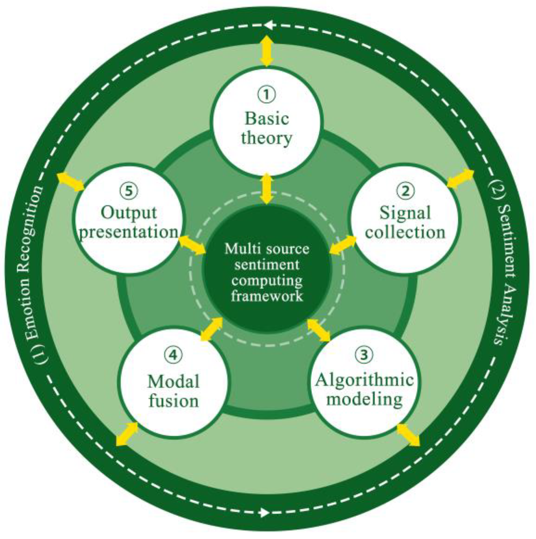
Figure 2.
Study areas and landscapes: (a) The location of Dalian in Liaoning Province; (b) The block of the three villages in the city of Dalian; (c) The location of the three villages in their respective blocks; (d) Specific locations of the three types of villages.
Figure 2.
Study areas and landscapes: (a) The location of Dalian in Liaoning Province; (b) The block of the three villages in the city of Dalian; (c) The location of the three villages in their respective blocks; (d) Specific locations of the three types of villages.
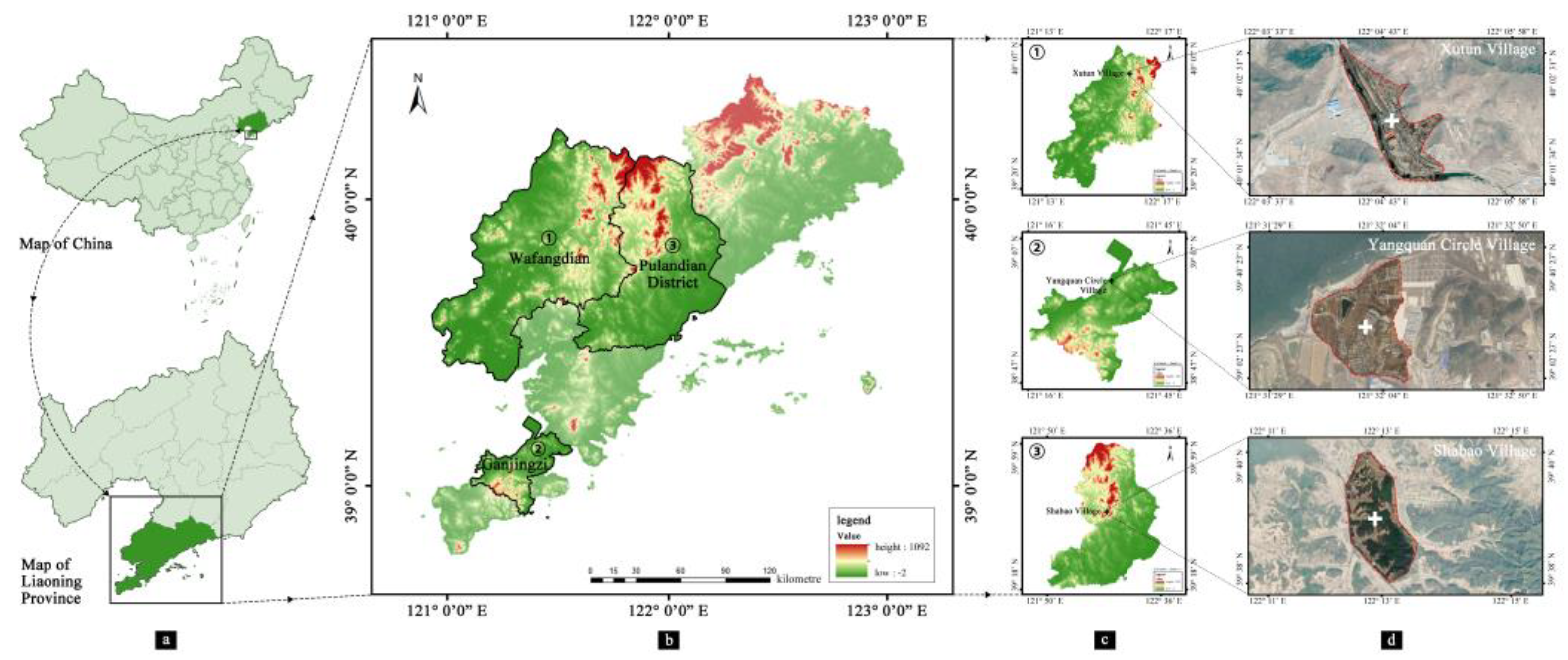
Figure 3.
Experimental elements presented in pictures. The first three acts of the three villages in the building, water, vegetation, road four types of landscape selection (A1-A12), the last act of the three preheating pictures of the experiment.
Figure 3.
Experimental elements presented in pictures. The first three acts of the three villages in the building, water, vegetation, road four types of landscape selection (A1-A12), the last act of the three preheating pictures of the experiment.
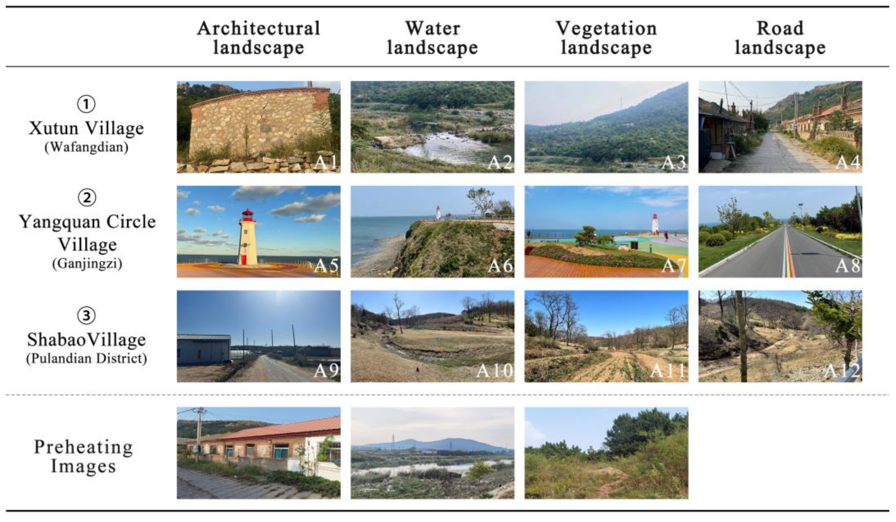
Figure 4.
Laboratory equipment drawing. It includes devices such as eye movements, EEG, signal amplifiers, display screens and laptops.
Figure 4.
Laboratory equipment drawing. It includes devices such as eye movements, EEG, signal amplifiers, display screens and laptops.
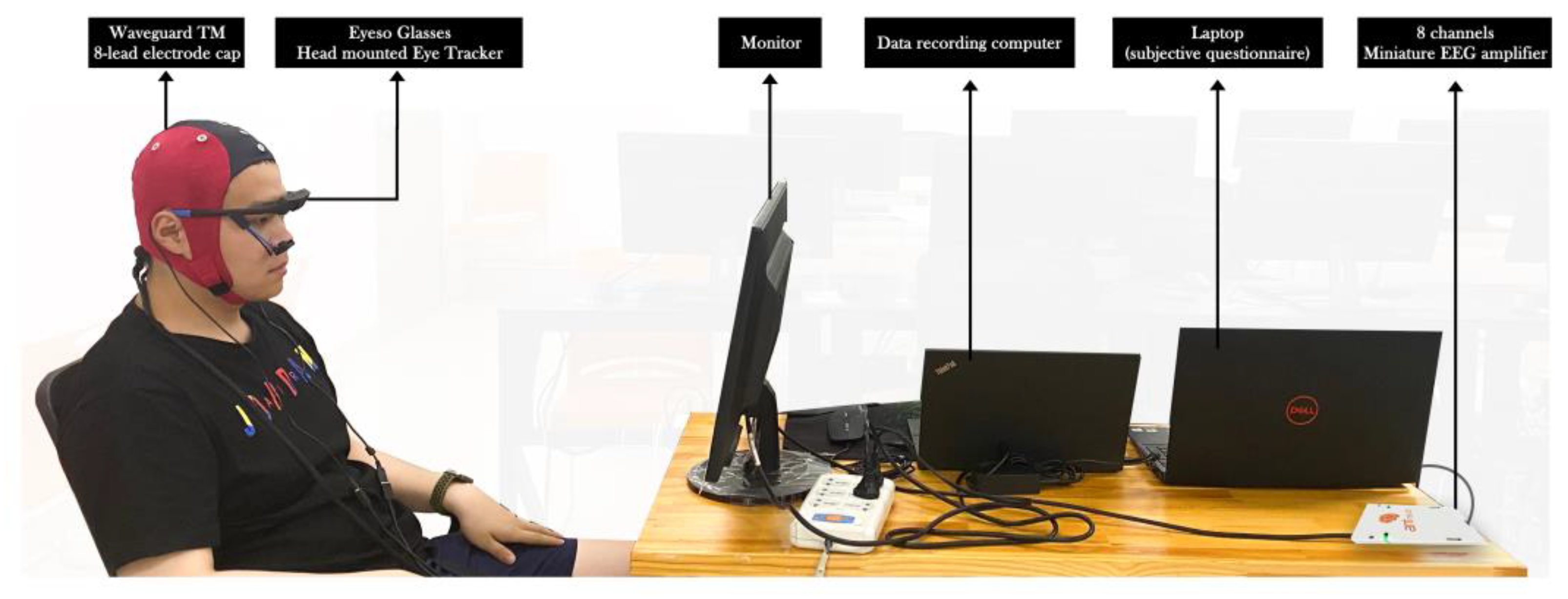
Figure 5.
Self-assessment Scale (SAM). Used to score the emotional dimension of price (first line), arousal (second line).
Figure 5.
Self-assessment Scale (SAM). Used to score the emotional dimension of price (first line), arousal (second line).
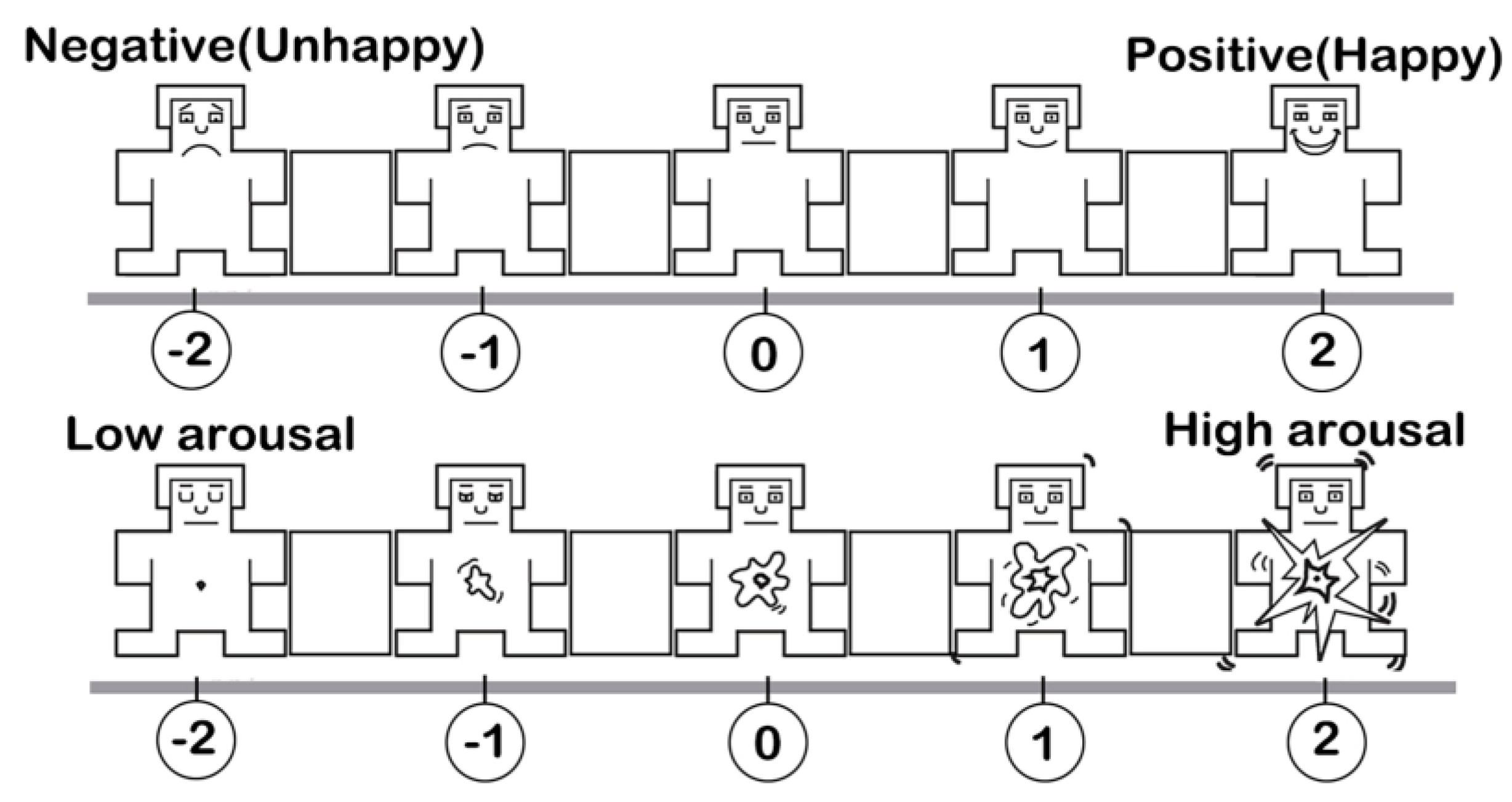
Figure 6.
Experimental program diagram. From experimental preparation (5-6min) to physiological data collection (6min), to the completion of two subjective questionnaires (10-15min).
Figure 6.
Experimental program diagram. From experimental preparation (5-6min) to physiological data collection (6min), to the completion of two subjective questionnaires (10-15min).
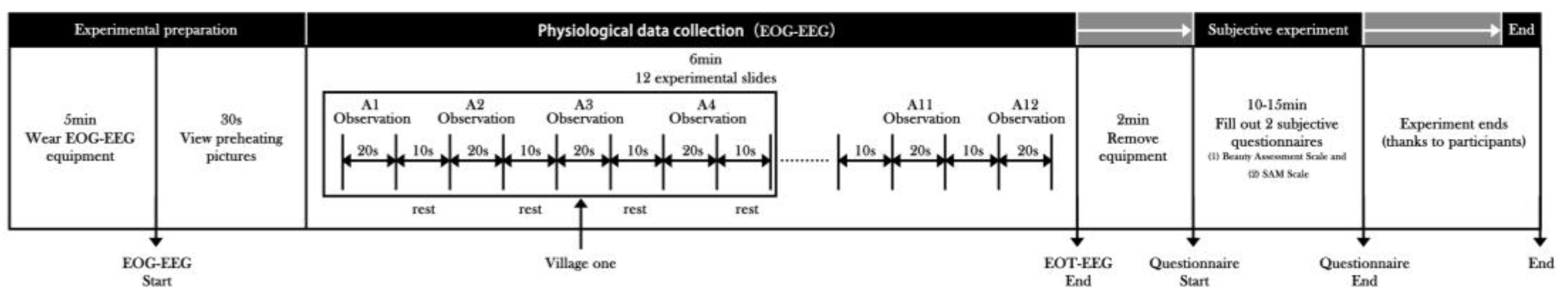
Figure 7.
Eye movement hot spot map. The concentration of gaze decreases from red and yellow to green.
Figure 7.
Eye movement hot spot map. The concentration of gaze decreases from red and yellow to green.
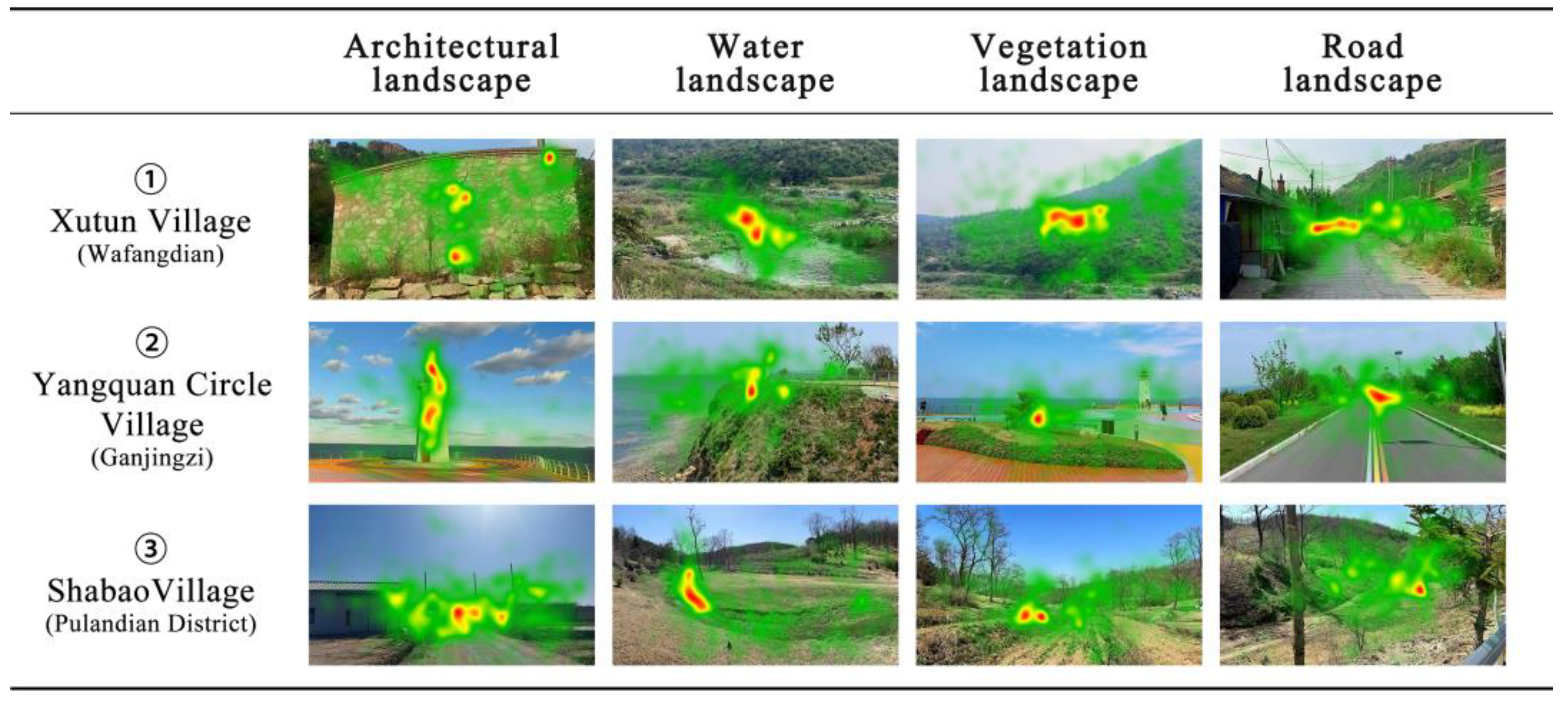
Figure 8.
Signal feature extraction diagram. The bold is the 36 indicators after feature extraction, and the italic is the deleted feature indicators.
Figure 8.
Signal feature extraction diagram. The bold is the 36 indicators after feature extraction, and the italic is the deleted feature indicators.
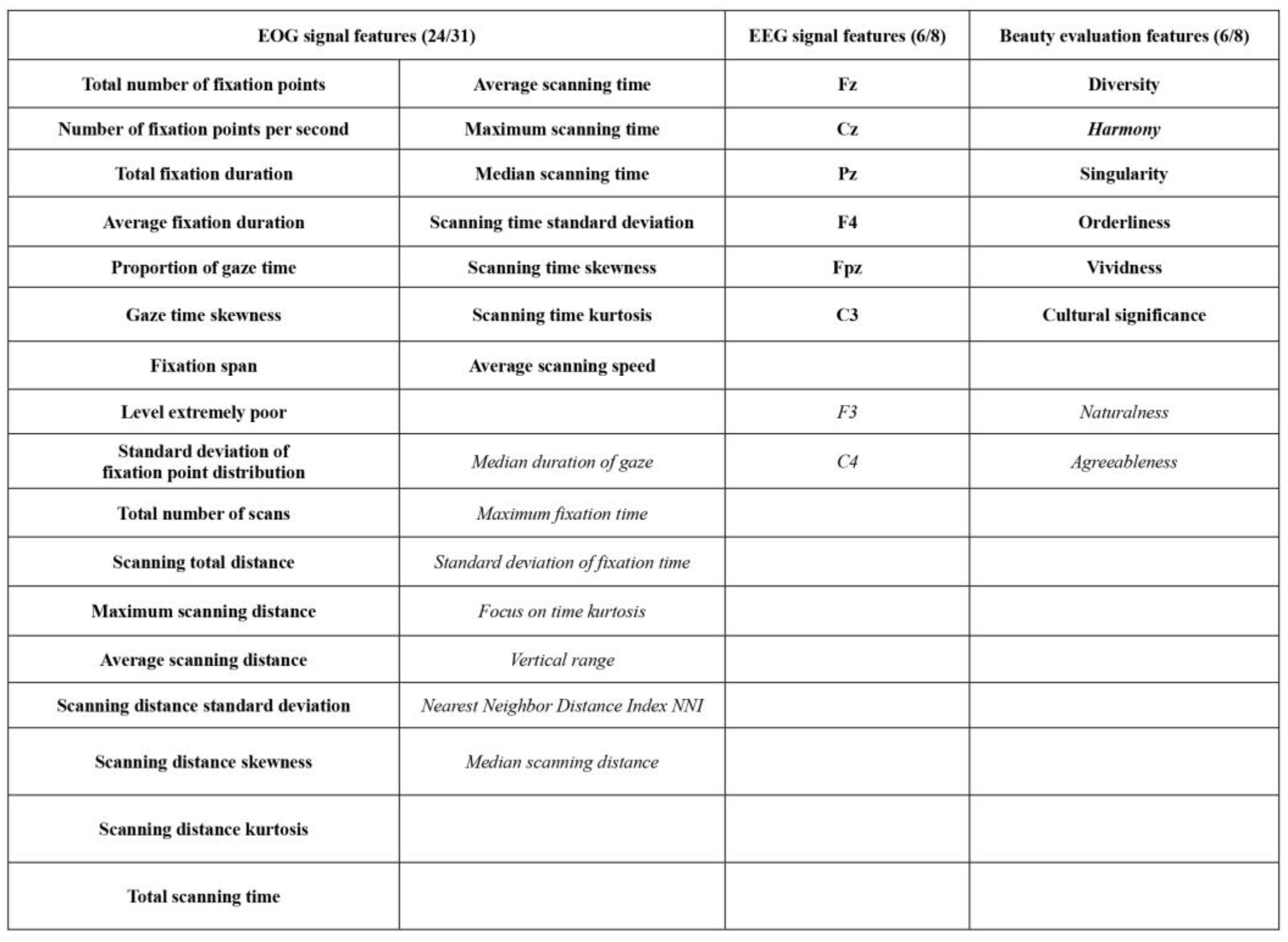
Figure 9.
Comparison of confusion matrix between valence and arousal binary classification models. The classifiers used are: (a) XGBoost; (b) RF; (c) DT; (d) LR-GD.
Figure 9.
Comparison of confusion matrix between valence and arousal binary classification models. The classifiers used are: (a) XGBoost; (b) RF; (c) DT; (d) LR-GD.
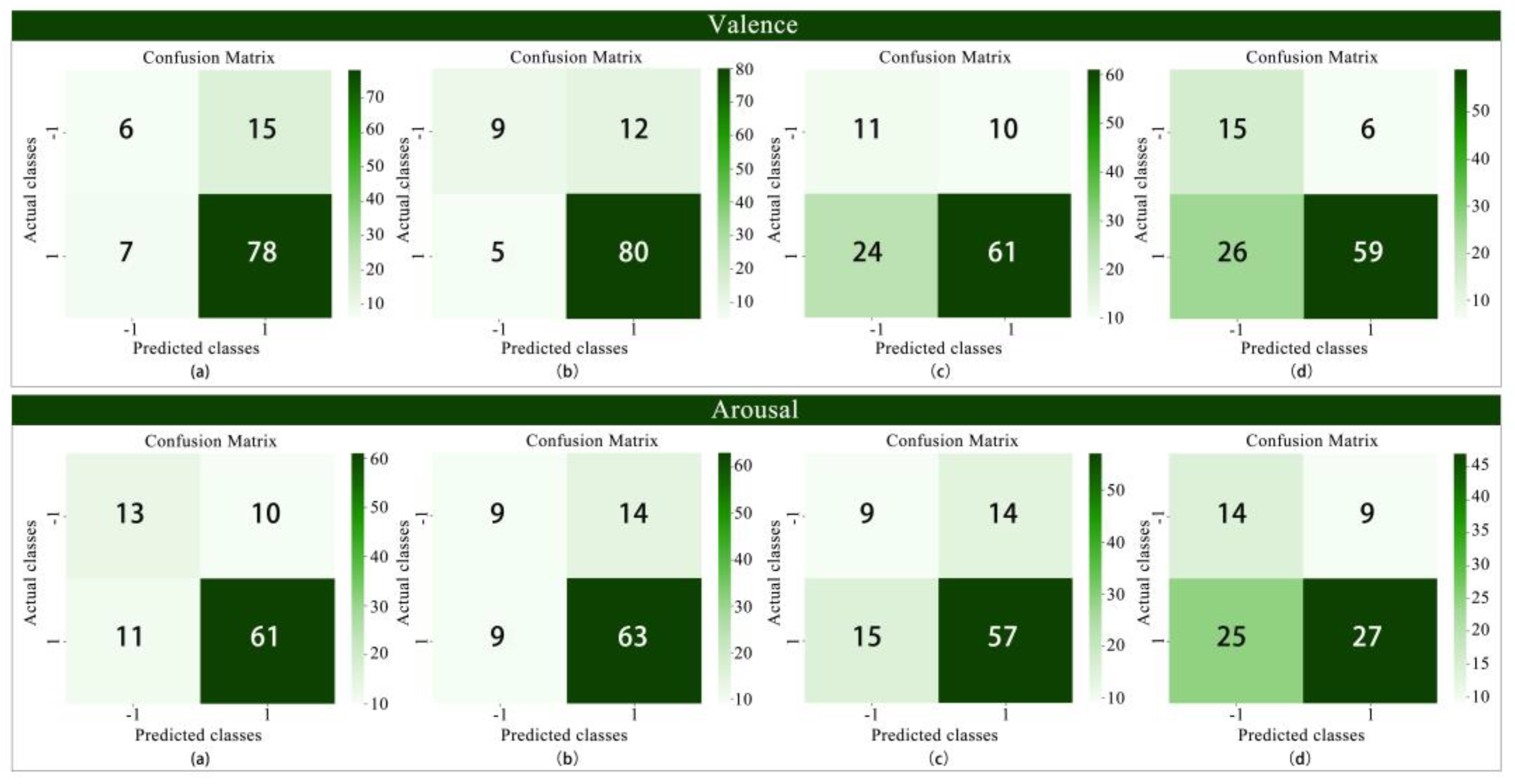
Figure 10.
Comparison of confusion matrix between valence and wake ternary classification model. The classifiers used are: (a) XGBoost; (b) RF; (c) DT; (d) LR-GD.
Figure 10.
Comparison of confusion matrix between valence and wake ternary classification model. The classifiers used are: (a) XGBoost; (b) RF; (c) DT; (d) LR-GD.
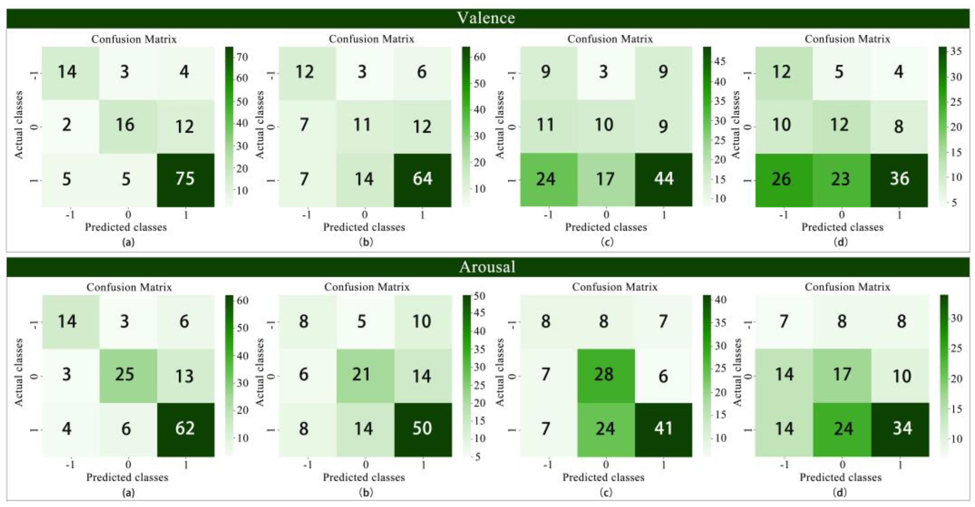
Figure 11.
Comparison of confusion matrix between valence and arousal five-element classification model. The classifiers used are: (a) XGBoost; (b) RF; (c) DT; (d) LR-GD.
Figure 11.
Comparison of confusion matrix between valence and arousal five-element classification model. The classifiers used are: (a) XGBoost; (b) RF; (c) DT; (d) LR-GD.
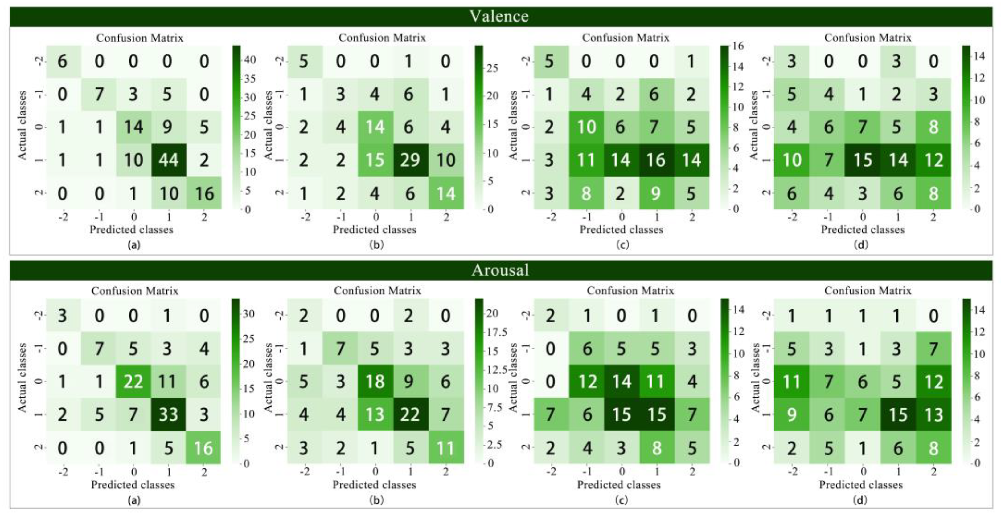
Figure 12.
Comparison of accuracy and main performance indexes of binary, ternary and five-element classification models of emotional valence.
Figure 12.
Comparison of accuracy and main performance indexes of binary, ternary and five-element classification models of emotional valence.
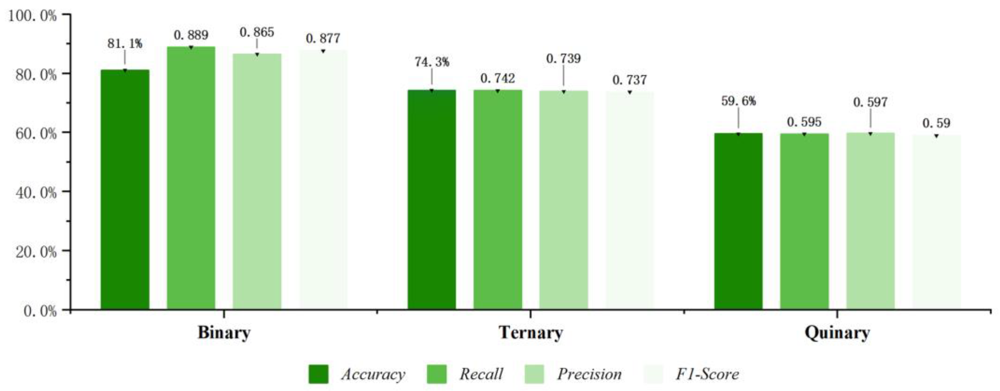
Figure 13.
Comparison of accuracy and main performance indexes of binary, ternary and five-element classification models of emotional arousal.
Figure 13.
Comparison of accuracy and main performance indexes of binary, ternary and five-element classification models of emotional arousal.
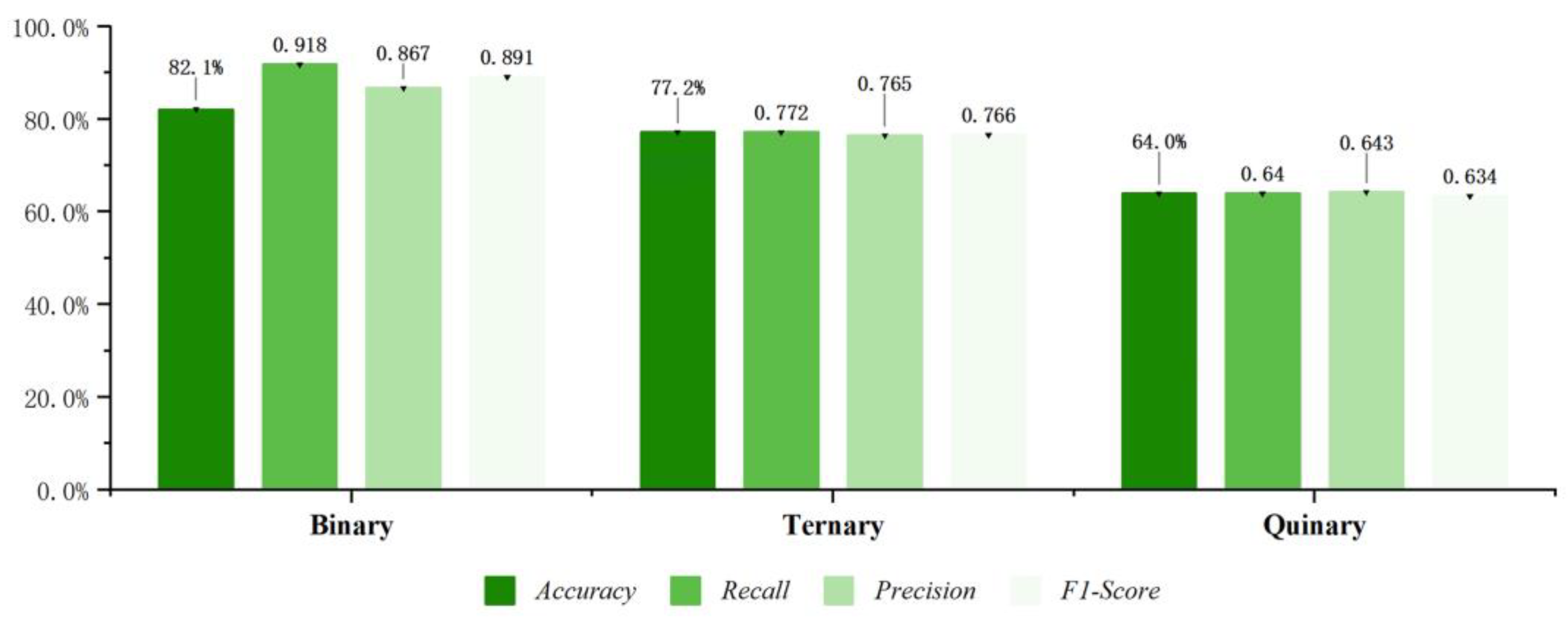
Figure 14.
Model experiment process diagram. The classifiers used are: (a) for the participants; (b) for the main evaluation process; (c) for the output of the evaluation decision.
Figure 14.
Model experiment process diagram. The classifiers used are: (a) for the participants; (b) for the main evaluation process; (c) for the output of the evaluation decision.
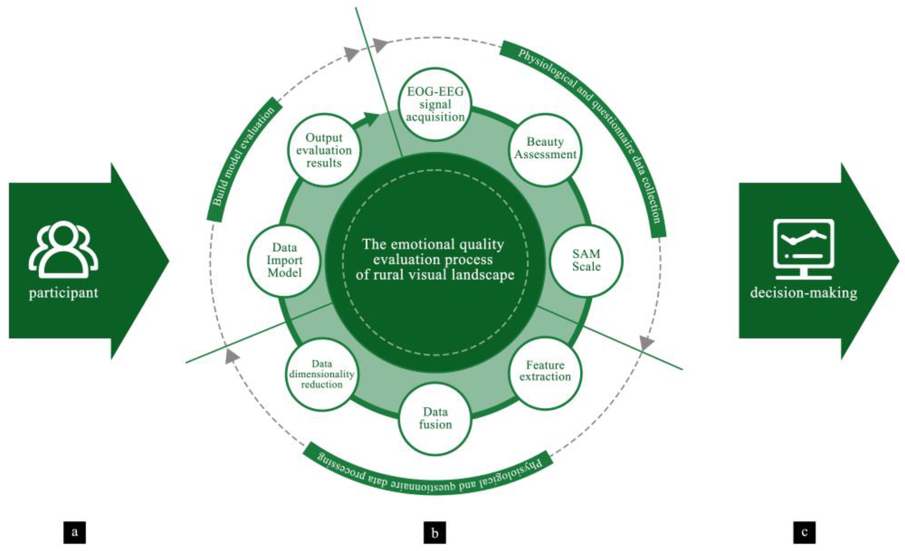

Table 1.
Beauty assessment data symmetric distribution test table.
| variable | skewness | kurtosis | minimum value | maximum value | average value | standard deviation |
|---|---|---|---|---|---|---|
| Naturalness | -0.752 | -0.306 | 1 | 5 | 3.80 | 1.156 |
| Diversity | -0.198 | -0.684 | 1 | 5 | 3.14 | 1.113 |
| Harmony | -0.244 | -0.761 | 1 | 5 | 3.32 | 1.135 |
| Singularity | 0.092 | -0.722 | 1 | 5 | 2.85 | 1.142 |
| Orderliness | -0.201 | -0.752 | 1 | 5 | 3.20 | 1.130 |
| Vividness | -0.202 | -0.487 | 1 | 5 | 3.24 | 1.064 |
| Culture | -0.185 | -0.636 | 1 | 5 | 3.09 | 1.104 |
| Agreeableness | -0.185 | -0.692 | 1 | 5 | 3.32 | 1.170 |
Table 2.
Comparison of model valence performance based on 47 features and 36 features.
| Class | Classifier | 47 features | 36 features | |||||||
|---|---|---|---|---|---|---|---|---|---|---|
| Accuracy | Recall | Precision | F1-Score | Accuracy | Recall | Precision | F1-Score | |||
| Binary | XGBoost | 79.3% | 0.918 | 0.839 | 0.876 | 82.1% | 0.918 | 0.867 | 0.891 | |
| RF | 79.3% | 0.918 | 0.839 | 0.876 | 84.0% | 0.941 | 0.870 | 0.904 | ||
| Ternary | XGBoost | 65.4% | 0.654 | 0.654 | 0.630 | 77.2% | 0.772 | 0.765 | 0.766 | |
| RF | 62.5% | 0.625 | 0.606 | 0.611 | 64.0% | 0.640 | 0.646 | 0.642 | ||
Table 3.
Comparison of model wake-up performance based on 47 features and 36 features.
| Class | Classifier | 47 features | 36 features | |||||||
|---|---|---|---|---|---|---|---|---|---|---|
| Accuracy | Recall | Precision | F1-Score | Accuracy | Recall | Precision | F1-Score | |||
| Binary | XGBoost | 77.9% | 0.847 | 0.859 | 0.853 | 81.1% | 0.889 | 0.865 | 0.877 | |
| RF | 75.8% | 0.875 | 0.818 | 0.846 | 76.8% | 0.875 | 0.829 | 0.851 | ||
| Ternary | XGBoost | 59.6% | 0.596 | 0.591 | 0.582 | 74.3% | 0.743 | 0.740 | 0.738 | |
| RF | 57.4% | 0.574 | 0.556 | 0.558 | 58.1% | 0.581 | 0.578 | 0.579 | ||
Table 4.
Performance comparison of binary classification models based on different classifiers for valence and arousal.
Table 4.
Performance comparison of binary classification models based on different classifiers for valence and arousal.
| Emotional category | Classifier | Accuracy | Recall | Precision | F1-Score |
|---|---|---|---|---|---|
| Valence | XGBoost | 82.1% | 0.918 | 0.867 | 0.891 |
| RF | 84.0% | 0.941 | 0.870 | 0.904 | |
| DT | 67.9% | 0.718 | 0.859 | 0.782 | |
| LR-GD | 69.8% | 0.694 | 0.908 | 0.787 | |
| Arousal | XGBoost | 81.1% | 0.889 | 0.865 | 0.877 |
| RF | 75.8% | 0.875 | 0.818 | 0.846 | |
| DT | 69.5% | 0.792 | 0.803 | 0.797 | |
| LR-GD | 64.2% | 0.653 | 0.839 | 0.734 |
Table 5.
Performance comparison of ternary classification models based on different classifiers for valence and arousal.
Table 5.
Performance comparison of ternary classification models based on different classifiers for valence and arousal.
| Emotional category | Classifier | Accuracy | Recall | Precision | F1-Score |
|---|---|---|---|---|---|
| Valence | XGBoost | 77.2% | 0.772 | 0.765 | 0.766 |
| RF | 64.0% | 0.640 | 0.646 | 0.642 | |
| DT | 46.3% | 0.463 | 0.549 | 0.490 | |
| LR-GD | 44.1% | 0.441 | 0.574 | 0.468 | |
| Arousal | XGBoost | 74.3% | 0.743 | 0.740 | 0.738 |
| RF | 58.1% | 0.581 | 0.578 | 0.579 | |
| DT | 56.6% | 0.566 | 0.604 | 0.572 | |
| LR-GD | 42.7% | 0.427 | 0.485 | 0.445 |
Table 6.
Performance comparison of valence and arousal five-element classification models based on different classifiers.
Table 6.
Performance comparison of valence and arousal five-element classification models based on different classifiers.
| Emotional category | Classifier | Accuracy | Recall | Precision | F1-Score |
|---|---|---|---|---|---|
| Valence | XGBoost | 64.0% | 0.640 | 0.643 | 0.634 |
| RF | 47.8% | 0.478 | 0.487 | 0.476 | |
| DT | 26.5% | 0.265 | 0.301 | 0.268 | |
| LR-GD | 26.5% | 0.265 | 0.335 | 0.278 | |
| Arousal | XGBoost | 59.6% | 0.596 | 0.598 | 0.590 |
| RF | 44.1% | 0.441 | 0.475 | 0.452 | |
| DT | 30.9% | 0.309 | 0.329 | 0.313 | |
| LR-GD | 24.3% | 0.243 | 0.349 | 0.265 |
Disclaimer/Publisher’s Note: The statements, opinions and data contained in all publications are solely those of the individual author(s) and contributor(s) and not of MDPI and/or the editor(s). MDPI and/or the editor(s) disclaim responsibility for any injury to people or property resulting from any ideas, methods, instructions or products referred to in the content. |
© 2025 by the authors. Licensee MDPI, Basel, Switzerland. This article is an open access article distributed under the terms and conditions of the Creative Commons Attribution (CC BY) license (http://creativecommons.org/licenses/by/4.0/).
Copyright: This open access article is published under a Creative Commons CC BY 4.0 license, which permit the free download, distribution, and reuse, provided that the author and preprint are cited in any reuse.


