
Submitted:
26 July 2024
Posted:
29 July 2024
You are already at the latest version
Abstract
Background: In recent years, computational aesthetics and neuroaesthetics have provided novel insights into understanding beauty. Building upon the findings of traditional aesthetics, this study aims to combine these two research methods to explore an interdisciplinary approach to studying aesthetics; Method: Abstract artworks were used as experimental materials. Based on traditional aesthetics and in combination, features of composition, tone, and texture were selected. Computational aesthetic methods were then employed to correspond these features to physical quantities: blank space, gray histogram, GLCM, LBP, and Gabor filters. An EEG experiment was carried out, in which participants conducted aesthetic evaluations of the experimental materials in different contexts (genuine, fake), and their EEG data was recorded to analyze the impact of various feature classes in the aesthetic evaluation process. Finally, a SVM was utilized to model the feature data, EEG data, context data, and subjective aesthetic evaluation data; Result: Behavioral data revealed that higher aesthetic ratings in the genuine context. EEG data indicated that genuine contexts elicited more negative deflections in the prefrontal lobes between 200-1000ms. Class II compositions demonstrated more positive deflections in the parietal lobes at 50-120ms, while Class I tones evoked more positive amplitudes in the occipital lobes at 200-300ms. Gabor features showed significant variations in the parieto-occipital area at an early stage. Class II LBP elicited a prefrontal negative wave with a larger amplitude. The results of the SVM models indicated that the model incorporating aesthetic subject and context data (ACC=0.76866) outperforms the model using only parameters of the aesthetic object (ACC=0.68657); Conclusion: A positive context tends to provide participants with a more positive aesthetic experience, but abstract artworks may not respond to this positivity. During aesthetic evaluation, the ERP data activated by different features show a trend from global to local. The SVM model based on multimodal data fusion effectively predicts aesthetics, further demonstrating the feasibility of the combined research approach of computational aesthetics and neuroaesthetics.
Keywords:
Aesthetics
; Computational Aesthetics
; Neuroaesthetics
; EEG
; ERP
; Support Vector Machine
1. Introduction
Since ancient times, human beings have been in pursuit of the essence of aesthetics. Alexander Gottlieb Baumgarten emphasized the subjectivity and individualization of the aesthetic experience, and he believed that the aesthetic feeling is the core of aesthetics, which refers to the direct experience and perception of beauty by human beings [1]. Aesthetics research encompasses a wide range of disciplines, including art, philosophy, and cultural studies. With the advancement of psychology, there has been a burgeoning interest in studying the brain's activities during the appreciation of art and the experience of beauty, with the goal of unraveling the neural mechanisms underlying aesthetic experience. Zeki first put forward the concept of neuroesthetics in the 1990s, with the aim of explaining and understanding the neural level of aesthetic experience through neural science [2]. Leder et al. [3,4] hold the belief that aesthetic experience is a dynamic process, encompassing the initial perceptual perception of sensory features such as color, shape, and texture, the understanding, interpretation, and evaluation of artworks, and the interaction and dynamic changes of emotions throughout the aesthetic process.
Research has indicated that there are certain commonalities in human visual cognitive mechanisms. For instance, stimulus symmetry may give rise to selective attention towards the overall characteristics of visual stimuli and facilitate higher-level cognitive processing in infants [5]. In the case of adults, a strong positive correlation is exhibited between symmetry judgment and aesthetic evaluation [6]. Certainly, it is not to imply that what is symmetrical is necessarily beautiful [7]. However, this inherent condition will, to a certain extent, affect people's aesthetic cognition. Additionally, acquired learning and the accumulation of experience will also have an impact on aesthetics. Untrained viewers tend to focus more on individual objects rather than the relationships between graphic elements in paintings. Trained viewers are capable of suppressing the natural inclination to concentrate on the subject and can detect patterns and relationships among compositional elements [8]. Zeki classified aesthetic experiences into two categories: biological beauty, which is determined by innate brain concepts that remain unchanged even with experience, and artificial beauty, which is determined by acquired concepts [9]. Aside from aesthetic experiences derived from sensory sources, factors like the environmental context of aesthetics can also have an impact on people's aesthetic perception. Research has indicated that the aesthetic scores assigned by subjects who viewed stimuli in a "gallery" setting were notably higher compared to those of subjects who viewed the stimuli in a "computer" environment [10]. Artworks displayed in museums tend to be more popular than those exhibited in laboratories [11].
It is commonly accepted that beauty is subjective and there is no absolute standard. Nevertheless, previous research has demonstrated that when experiencing beautiful works, different observers tend to share certain similarities, and they show a preference for works with specific characteristics. George David Birkhoff put forth an attempt to quantify aesthetics: [12]. The two physical quantities of complexity, and order(entropy) can be linked to traditional beauty concepts in art history. Liu et al. [13] introduced the concept of "Engineering Aesthetics," which integrates the aesthetic dimension into ergonomics. The objective is to employ engineering and scientific approaches to investigate aesthetics and incorporate these methods into the aesthetic design and evaluation process. In such instances, methods of statistical physics and network science can be used to quantify and to better understand what it is that evokes that pleasant feeling [14]. In 2005, at the international academic conference on Computational Aesthetics in Graphics, Visualization, and Imaging of the Eurographics Association, Computational Aesthetics was initially put forward. Computational Aesthetics is the research of computational methods that can make applicable aesthetic decisions in a similar fashion as humans can)[15]. The advantage of Computational Aesthetics lies in its ability to quantify various abstract aesthetic features, such as style, texture features, and so on [16]. By investigating the connection between these features and beauty, researchers are able to undertake tasks such as classification learning through the utilization of modelling techniques like Convolutional Neural Networks (CNN), Support Vector Machines (SVM), and Back Propagation (BP) neural networks [17,18,19]. In addition to quantifying the aesthetic object, researchers have also started to incorporate more factors as the aesthetic subject. This includes combining visual and text data for quantification [20] , analyzing the emotions in paintings [21], and optimizing the model by integrating eye movement data , and optimizing the model by integrating eye movement data [22].
It can be observed that computational aesthetics excels at using mathematical methods to quantify the features of aesthetic objects. Subsequently, various mathematical techniques are employed to build models that simulate human aesthetic evaluations. Neuroaesthetics, on the other hand, primarily focuses on the study of the aesthetic subject. It employs psychological methods to investigate different aesthetic mechanisms and the impact of features, contexts, and other factors on aesthetics. This study proposes to integrate the research methods of computational aesthetics and neuroaesthetics to explore a comprehensive research approach. This approach involves delving into the internal relationships between features and aesthetics, as well as integrating and modeling the multimodal data of the aesthetic subject, aesthetic object, and aesthetic context. By leveraging the strengths of computational aesthetics in feature extraction and the advantages of neuroaesthetics in cognitive research, we aim to develop a more holistic understanding of aesthetic evaluation.
Representational paintings have been proved to have higher judgments on the perceptual dimensions of the semantic dimension of the Illusion of Reality [23]. Therefore, this study employed abstract artworks as experimental materials. The specific methods are as follows:
First, based on traditional concepts in art history, computational aesthetics is used to analyze and quantify the physical quantities corresponding to different features. Previous research has indicated that in the process of human visual perception, global processing is completed before more local analysis, that is, the Global Precedence Hypothesis: People typically perceive global features first in the visual processing and then notice local details [24,25,26,27]. Love et al. [28] discovered via eye movement research that even when the local and global forms have equal conspicuity, there remains an advantage in the processing of the overall form. Of course, the global advantage also has individual differences. Expertise would affect saccade metrics, biasing them towards larger saccade amplitudes, artists adopted a more global scan path strategy when performing a task related to art expertise [29,30,31]. Global features encompass the arrangement and interrelationships of diverse visual elements within an artwork, and this overall relationship can be summarized as the composition of the picture [32,33]. Different compositions yield different visual effects. A good composition necessitates the rational allocation of subject space and negative space to achieve simplicity and balance. For instance, in traditional Chinese painting, a significant amount of blank space is frequently utilized to guide the viewer's attention, create dynamic visual balance, enhance the rhythm of the picture, and generate a simple and ethereal ambiance [34,35].
Within the realm of painting, photography, and other visual arts, tone is an additional crucial global feature. It indicates the lightness and darkness within the grayscale of an image. By manipulating the tone's lightness and darkness, contrast, and distribution, the overall style and emotional expression of the work can be influenced. Understanding and mastering the harmony of tone values and colors is of great significance for artists and photographers in capturing the beauty of nature. Furthermore, the tone value of an artwork can be influenced by the environment, and the same tone value work may also generate different aesthetic appraisals and viewing comforts under various lighting conditions [36,37,38].
Aside from the overall composition and tone, various detailed textures in artworks can also have an impact on aesthetics. While the texture in traditional art aesthetics and the texture in computational aesthetics both describe and analyze the structure and pattern of images, they differ significantly in terms of methods, applications, and evaluation criteria. The texture in traditional aesthetics places greater emphasis on subjective experience and artistic expression, whereas the texture in computational aesthetics emphasizes objective analysis and computational feature extraction. Computational aesthetics can correlate abstract artistic features with those that impact aesthetics in a quantitative manner, such as using the Gray Level Co-occurrence Matrix (GLCM) to identify the texture/surface quality in traditional aesthetics that reflects the visual and tactile sensations of the surface (smoothness, roughness, softness, hardness, etc.)[39], using the Local Binary Patterns (LBP) to quantify the details/intricacy in art works [40], and using Gabor filters to extract repetition and rhythm in the picture through frequency domain analysis[41], etc.
This study adheres to the general principles of Global Precedence Hypothesis and quantifies the features of artworks from three aspects: composition, tone, and texture (both global and local).
Second, based on the quantitative results, cluster analysis of the stimulus materials is performed, and the tagging method is used to classify the stimulus materials.
Third, using the research method of neuroaesthetics, an electroencephalogram (EEG) experiment is conducted to analyze the influence of different classes of features in the process of aesthetic evaluation.
Finally, by utilizing the research method of computational aesthetics, we fuse and model the multimodal data, incorporating the feature data of the stimulus materials (aesthetic object), the Event-Related Potentials (ERP) data of the participants (aesthetic subject), and the aesthetic context data, to construct a machine learning model. By employing this interdisciplinary approach, we enhance our understanding of the cognitive processes involved in the evaluation of different types of features and build machine learning models to simulate and predict human aesthetic preferences.
2. Materials and Methods
In this study, Visual Studio 2019 and the Open Source Computer Vision Library (OpenCV) are utilized to perform grayscale processing on artworks, followed by feature quantization.
2.1. Features
2.1.1. Composition
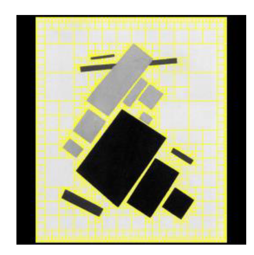
In an artistic creation, a rational composition of the image can be attained by appropriately distributing the foreground, background, primary and secondary objects, etc. Some research has adopted the QuadTrees approach to quantify the blank space characteristics of images, and experiments have demonstrated that it is related to the complexity of the picture and will have an impact on the viewer's attention [42]. QuadTrees is a commonly used data structure for recursively subdividing a two-dimensional space into four quadrants or regions, thereby partitioning the two-dimensional space. By dividing the region into four equal quadrants, sub-quadrants, and so on to represent the division of the two-dimensional space, each leaf node contains data corresponding to a specific sub-region [43]. Based on the characteristics of abstract artworks, this study quantifies the blank space composition features using QuadTrees. The specific process is as follows: (1) Employ the average gray level of the image as the binarization threshold for image binarization processing; (2) Calculate the proportion of the black and white areas in the binarized image. Considering that the visual weight of dark colors is relatively large, in this experiment, if the black area in the binarized image exceeds 45%, then black is used as the blank space, otherwise, white is used as the blank space; (3) Utilize the QuadTrees method to quantify the ratio of the blank area to the total area of the image, and obtain the blank area ratio.
Figure 1.
The calculation of blank space in Suprematist Composition: Airplane Flying (Images processed by authors as fair use from wikiart.org).
Figure 1.
The calculation of blank space in Suprematist Composition: Airplane Flying (Images processed by authors as fair use from wikiart.org).
2.1.2. Tone
In this study, the tone is quantified through the utilization of the gray histogram. This histogram calculates the quantity of pixels at each gray level present in the image, and subsequently, the pixels in the image are tallied based on their respective gray levels and presented in the form of a histogram. By quantifying the characteristics of the gray histogram, the tone of the image can be reflected from multiple facets.
Mean: The average of the gray levels in the histogram, which represents the overall brightness level of the image.
Variance: Describes the degree of dispersion of the histogram, that is, the extent to which the gray levels deviate from the mean of the histogram.
Skewness: Describes the asymmetry of the histogram. A positive skewness indicates that the tone value in the image is higher; a negative skewness indicates that the tone value in the image is lower.
Kurtosis: Describes the peakedness of the histogram. A positive kurtosis indicates that the gray values in the image are concentrated in certain specific gray levels. A kurtosis of 0 indicates that the peak of the data distribution is similar to that of the standard normal distribution.
Energy: The sum of the squares of the pixel counts at each gray level in the histogram, which reflects the uniformity of the gray level distribution in the image. A higher energy indicates that the gray level distribution in the image is more even.
represents the number of gray levels, denotes the frequency of the gray level, and indicates the size of the picture (total number of pixels).
2.1.3. Global Texture Features
A large number of local features, through rational distribution and integration, become the global texture features of the work. The overall texture features can be reflected through the spatial frequency. The spatial frequency of a picture describes the frequency of changes in texture, details, structure, etc. at various spatial locations in the image.
In this study, Gabor filters are utilized to extract the overall texture features of the image. By applying Gabor filters on different scales and orientations, the texture features of the entire image are obtained. The Gabor operator can acquire texture features of different frequencies and angles, and can capture local spatial frequency and orientation information in the image:
Complex:
Real:
Imaginary:
where:
Here, represents the wavelength, represents the direction, represents the phase offset, represents the aspect ratio of the space, and is the variance of the Gaussian filter. The mathematical expression for applying the Gabor filter to the image is a convolution operation:
Here, represents the convolution operation, and is the filtered image. The parameters of the filter are set as follows: , and different wavelengths and angles are used, as shown in Figure 2. The mean, variance, and energy of the filtered image are calculated (refer to the calculation formulas (1), (2), and (5)).
The mean value indicates the presence of obvious edges or textures in the original image at that wavelength and angle. The variance of the processed image reflects the degree of dispersion of the image gray level, that is, the complexity of the texture. The energy value of the processed image reflects the uniformity of the image texture.
and angles .
2.1.4. Local Texture Features
In the realm of artistic creation, creators manipulate the texture of each area to generate diverse visual effects in the picture. Through the integration of the interrelationships among various components, a complete work is ultimately fashioned. For the extraction of local texture features, this study makes use of two extraction techniques: the Gray-Level Co-occurrence Matrix (GLCM) and the Local Binary Pattern (LBP).
Gray-Level Co-Occurrence Matrix (GLCM)
Through the analysis of the gray-level relationship between pixel pairs (or pixel neighbor pairs) in the image, the texture information of the image is captured. This reflects the spatial distribution relationship between different gray levels in the image.
Suppose the gray level range of the image is from 0 to L-1,the GLCM is an L×L matrix, where L represents the number of gray levels. The element in the GLCM indicates the frequency of occurrence of gray level and gray level in a specific spatial relationship within the image. For each pixel in a specific spatial relationship within the image. For each pixel , the neighboring pixel at a distance d is examined. The frequency of occurrence of the pixel pair is counted, and the count at the corresponding position in the GLCM is incremented by 1:
where denotes the coordinate of the neighboring pixel of the pixel at a distance d and in the direction . By quantifying the features of the GLCM, the texture of the image is reflected from multiple aspects. The degree of contrast between pixels with higher gray levels and pixels with lower gray levels in the GLCM. It reflects the contrast and roughness of the texture of the image.
Energy: The square of the sum of the probabilities between pixel pairs in the GLCM, which reflects the uniformity of the image texture (refer to the calculation formula (5)).
Entropy: The uncertainty of the probability distribution between pixel pairs in the GLCM, which reflects the complexity of the image texture.
Local Binary Pattern (LBP)
The fundamental principle of the LBP feature is to obtain a local binary coding for each pixel in the image by comparing its gray value with the neighboring pixels in the surrounding area. This is used to represent the texture feature of the pixel. For a specific pixel point in the image, a circular neighborhood with a radius of R is defined, which contains P sampling points and can be expressed as:
where .
For each pixel point in the image, the LBP code is computed as follows:
where, represents the gray value of the pixel point ; represents the gray value of the central pixel , and is a step function that compares the gray value of each neighboring pixel with the gray value of the central pixel. If the gray value of the neighboring pixel is greater than or equal to the gray value of the central pixel, the pixel is marked as 1; otherwise, it is marked as 0:
In this study, the 8-neighborhood LBP operator with is utilized, so the LBP coding value range is 0-255. The histogram quantization method is employed to quantify the mean, variance, skewness, kurtosis, and energy of LBP as the quantization result of LBP, and then the image texture features are analyzed (refer to the calculation formulas (1) (2) (3) (4) (5)).
2.2. Stimulus
In order to avoid the influence of elements such as people, expressions, scenes, and landscapes in the image, this experiment selected abstract art works as stimulus materials. Through the website https://www.wikiart.org/, after searching with keywords of abstract styles such as constructivism, minimalism, neoplasticism, and suprematism, 249 abstract art works that met the experimental requirements were downloaded and sorted. Visual Studio 2019 software and OpenCV were used for image processing. First, the images were uniformly scaled to the largest size within 500×600 pixels, and the images were uniformly grayscale, with a resolution of 300dpi.
After quantifying the different feature data of 249 materials, a second-order cluster analysis was performed on the data of different features, and each image was classified using the label method. The results are shown in Table 1, Figure 3, Appendix A, and Appendix B.
2.3. EEG and ERP
In 1924, Hans Berger discovered EEG by positioning electrodes on the scalp and amplifying the signals to measure the electrical activity of the human brain [44]. In 1964, Gray Walter and his colleagues reported the first cognitive ERP component, namely, the contingent negative variation [45]. EEG reflects thousands of concurrent brain processes, among which the brain's response to a single stimulus or point of interest is typically undetectable in a single-trial EEG recording. By performing multiple trials and superimposing and averaging the results, the random brain activity can be averaged out, and the relevant waveforms, namely ERP, can be retained.
The electrode distribution selected for the EEG experiment is the international 10-20 system, and each electrode placement site has a letter to identify the corresponding brain lobe or region: prefrontal (Fp), frontal (F), temporal (T), parietal (P), central (C), and occipital (O). "Z" (zero) refers to the electrodes placed on the midline sagittal plane of the skull (Fpz, Fz, Cz, Oz), and even electrodes (2, 4, 6, 8) indicate that the electrodes are placed on the right side of the head, while odd electrodes (1, 3, 5, 7) indicate that the electrodes are placed on the left; M (also known as A) refers to the mastoid process, a prominent bony protuberance usually found behind the outer ear, and M1 and M2 are used for contralateral reference of all EEG electrodes.
2.4. Participants
In this study, 16 graduate students were recruited as participant s, all of whom were from the College of Mechanical Engineering and Automation, Huaqiao University. Among them, 12 were male participants and 4 were female participants, with an age range of 22 to 30 years old. All participants were right-handed, had no history of mental illness, had normal or corrected-to-normal vision, and had not received systematic aesthetic education. Prior to the experiment, the researchers had thorough communication with the participants, and the participants also signed the informed consent form. As compensation for their participation, each participant received 50 RMB. This experiment has been approved by the School of Medicine, Huaqiao University.
2.5. Procedure
In the EEG experiment, the participants placed their right hands on the mouse and were informed that the experimental materials were from the works of artists (“Genuine”) and the works copied by students (“Fake”) (in fact, all the works were from the works of artists). After fully understanding the content of the experiment, the participants needed to concentrate. First, the participants fixated on a white cross on a gray background for 800ms. Then, a context cue word (Genuine/Fake) would appear in the center of the screen for 1000ms. Next, an art work would be presented on the screen for 2000ms. After the participants appreciated it, a rating scale ranging from 1 to 5 appeared below the image, and participants used a mouse to click and evaluate the artwork's appeal (1: very unappealing; 5: very appealing). The scoring time was not limited, so the participants had sufficient time to respond. After the subjects clicked, an 800ms blank stimulus would appear, and the subjects could take an appropriate rest before entering the next cycle. The entire experiment was divided into 3 blocks, each containing 80 trials, and there was a rest of at least 5 minutes between each block. Before the main experiment, there would be a practice block containing 10 art works (which would not appear in the main experiment) to familiarize the participants with the experimental process.
The EEG data were recorded using a Neuroscan Synamp2 Amplifier, with the bilateral mastoids (M1, M2) serving as references. Additionally, two pairs of electrodes were utilized to record the vertical electrooculogram (VEOG) and horizontal electrooculogram (HEOG). The VEOG electrodes were positioned above and below the left eye, respectively, while the HEOG electrodes were placed 1 cm away from the outer corner of each eye. During the entire experiment, the impedance between the electrodes and the scalp was kept below 10kΩ to guarantee the quality of signal recording. Upon the completion of continuous EEG recording, offline data processing was carried out. The processing steps encompassed segmenting the EEG data, eliminating artifacts, superimposing and averaging, and performing baseline correction. The bandpass filter range was set at 0-30 Hz, and the EEG artifact removal criterion was ±100μV. Subsequently, the EEG recordings were divided into 1200ms epochs, spanning from 200ms before stimulus onset to 1000ms after stimulus onset, with the 200ms period prior to stimulus onset serving as the baseline.
For the average amplitude of each time window of ERP data, a repeated measures analysis of variance (ANOVA) was performed with the factors of task (aesthetic, balance), answer (yes, no), and 60 channels.
3. Results
Since the EEG data availability rate of 4 participants was less than 75%, only the EEG data of 12 participants were retained for subsequent analysis (with an average data availability of 91.8%).
3.1. Behavioral Data
A repeated measures ANOVA was performed to examine the effect of different contexts on the final aesthetic evaluation. The results demonstrated a significant difference in the aesthetic evaluation results across different contexts [F (1, 11) = 5.670, p = 0.036]. The average score in the genuine context (3.081 ± 0.097) was significantly higher than that in the fake context (2.890 ± 0.071).
3.2. EEG Data
3.2.1. Result of Context
As depicted in Figure 5, a more negative deflection for genuine context was observed in the prefrontal lobes within the time window between 200 and 1000ms. A repeated measures ANOVA was executed on the time window with factors of channel (60) × context (genuine, fake). The findings indicated that the main effect of context was significant [F (1, 11) = 4.941, p = 0.048 < 0.05], while the interaction of channel × context was also significant [F (59, 649) = 2.832, p < 0.01]. Further analysis revealed that in the FPZ channel, in comparison to the fake context, the genuine context would evoke a more negative amplitude [F (1, 11) = 11.902, p = 0.005 < 0.01], and a comparable waveform also manifested in the FP1 channel [F (1, 11) = 5.274, p = 0.042] and FP2 channel [F (1, 11) = 10.213, p = 0.009 < 0.01].
3.2.2. Result of Composition
As depicted in Figure 6, a more positive deflection for Class II composition was observed in the parietal lobes within the time window between 50 and 120ms. A repeated measures ANOVA was performed with factors of channel (60) × context (genuine, fake) × composition (Class I, Class II). The findings demonstrated that the main effects of context (F < 1) and composition (F < 1) were not significant, and neither was the interaction (F < 1). However, the interaction between channel and composition was significant [F (59, 649) = 2.657, p < 0.01], as was the interaction between channel × context × composition [F (59, 649) = 2.345, p < 0.01]. Further analysis revealed that in the PZ channel, the amplitude of the Class II composition was greater [F (1, 11) = 7.502, p = 0.019], and this was more pronounced in the genuine context [F (1, 11) = 14.784, p = 0.003]. Similarly, in the POZ channel, the amplitude of the Class II composition was also larger [F (1, 11) = 7.911, p = 0.017], and it was again more significant in the genuine context [F (1, 11) = 9.884, p = 0.009].
3.2.3. Result of Tone
As depicted in Figure 7, a more positive deflection for Class I tone was observed in the occipital lobes within the time window between 200 and 300ms. A repeated measures ANOVA was performed with factors of channel (60) × context (genuine, fake) × tone (Class I, Class II). The results indicated that the main effect of tone (F < 1), the interaction of context × tone (F < 1), and the interaction of channel × context × tone was not significant (F < 1), but the interaction of channel × tone was significant [F (59, 649) = 1.464, p = 0.016 < 0.05]. Further analysis revealed that in the OZ channel, Class I tone evoked a more positive going amplitude, relative to the Class II [F (1, 11) = 5.288, p = 0.042].
3.2.4. Result of Gabor-Mean
As depicted in Figure 8, in the center and left side of the parietal-occipital lobe, a more positive going deflection for Class II Gabor-Mean was observed within the time window between 70 and 130ms. A repeated measures ANOVA was conducted with factors of channel (60) × context (genuine, fake) × Gabor-Mean (Class I, Class II). The results suggested that the interaction of channel × Gabor-Mean was significant [F (59, 649) = 1.444, p = 0.020]. Further analysis revealed that in the PO3 channel, in comparison to the Class I Gabor-Mean, the Class II evoked a more positive amplitude [F (1, 11) = 5.972, p = 0.033]. A similar waveform was also observed in the PO5 channel [F (1, 11) = 6.651, p = 0.026], PO7 channel [F (1, 11) = 6.252, p = 0.029], and P7 [F (1, 11) = 5.518, p = 0.039]. No other effect was significant.
3.2.5. Result of Gabor-Variance
As depicted in Figure 9, in the center of the parietal lobe and parieto-occipital lobe, a more positive going deflection for Class II Gabor-Variance was observed within the time window between 70 and 130ms. A repeated measures ANOVA was conducted with factors of channel (60) × context (genuine, fake) × Gabor-Variance (Class I, Class II). The results suggested that the interaction of channel × Gabor-Variance was significant [F (59, 649) = 1.590, p = 0.004]. Further analysis disclosed that in the PZ channel, in comparison to the Class I Gabor-Variance, the Class II would evoke a more positive amplitude [F (1, 11) = 4.937, p = 0.048]. There was a marginally significant difference in the POZ channel [F (1, 11) = 4.722, p = 0.053]. No other effect was significant.
3.2.6. Result of Gabor - Energy
As depicted in Figure 10, in the center and right side of the parietal lobe and parieto-occipital lobe, a more positive going deflection for Class I Gabor- Energy was observed within the time window between 70 and 130ms. A repeated measures ANOVA was conducted with factors of channel (60) × context (genuine, fake) × Gabor-Energy (Class I, Class II). The results suggested that the interaction of channel × Gabor- Energy was significant [F (59, 649) = 2.020, p < 0.01]. Further analysis disclosed that in the PZ channel, in comparison to the Class II Gabor-Energy, the Class I would evoke a more positive amplitude [F (1, 11) = 14.109, p = 0.003]. A similar waveform was also observed in the POZ channel [F (1, 11) = 17.687, p = 0.001], P2 channel [F (1, 11) = 9.158, p = 0.012], P4 channel [F (1, 11) = 9.140, p = 0.012], PO4 channel [F (1, 11) =7.874, p = 0.017], and PO6 channel [F (1, 11) = 4.914, p = 0.049]. No other effect was significant.
A more positive going deflection for Class I Gabor- Energy was observed in the center of the parieto-occipital lobe within the time window between 200 and 300ms. A repeated measures ANOVA was conducted with factors of channel (60) × context (genuine, fake) × Gabor-Energy (Class I, Class II). The results suggested that the interaction of channel × Gabor- Energy was significant [F (59, 649) = 1.712, p = 0.001]. Further analysis disclosed that in the POZ channel, in comparison to the Class II Gabor-Energy, the Class I would evoke a more positive amplitude [F (1, 11) = 4.768, p = 0.052]. No other effect was significant.
3.2.7. Result of Horizontal GLCM (θ=0°)
As depicted in Figure 11, a more negative deflection for Class I horizontal GLCM was observed in the occipital lobe within the time window between 500 and 1000ms. A repeated measures ANOVA was conducted with factors of channel (60) × context (genuine, fake) × horizontal GLCM (Class I, Class II), which revealed an effect of horizontal GLCM [F (1, 11) = 5.112, p = 0.045]. Class I horizontal GLCM evoked a more negative going amplitude, compared to the Class II. The interaction of channel × horizontal GLCM was significant [F (59, 649) = 1.516, p < 0.01]. Further analysis uncovered that in the OZ channel, Class I horizontal GLCM evoked a more negative going amplitude [F (1, 11) = 5.332, p = 0.041]. No other effect was significant.
3.2.8. Result of Diagonal GLCM (θ=135°)
As depicted in Figure 12, a more negative deflection for Class I diagonal GLCM was observed in the left side of the parietal-occipital lobe within the time window between 70 and 140ms. A repeated measures ANOVA with the factors channel (60), context (genuine, fake), and diagonal GLCM (Class I, Class II), the interaction of channel × diagonal GLCM was significant [F (59, 649) = 1.444, p = 0.020]. Further analysis uncovered that in the PO5 channel, the amplitude of the Class I diagonal GLCM was greater [F (1, 11) = 6.651, p = 0.026]. Similarly, in the PO7 channel, the amplitude of the Class I diagonal GLCM was also larger [F (1, 11) = 6.252, p = 0.029]. No other effect was significant.
A more negative deflection for Class I diagonal GLCM was observed in the occipital lobes within the time window between 300 and 1000ms. A repeated measures ANOVA was conducted with factors of channel (60) × context (genuine, fake) × diagonal GLCM (Class I, Class II), which revealed an effect of diagonal GLCM [F (1, 11) = 5.070, p = 0.046]. Class I diagonal GLCM evoked a more negative going amplitude, compared to the Class II. The interaction of channel × diagonal GLCM was significant [F (59, 649) = 1.658, p = 0.02]. Further analysis uncovered that in the OZ channel, the wave amplitude induced by Class I was larger [F (1, 11) = 6.495, p = 0.027]. No other effect was significant.
3.2.9. Result of LBP
As depicted in Figure 13, a more negative going deflection for genuine context was observed in the center and left side of the frontal lobe within the time window between 300 and 1000ms. A repeated measures ANOVA was executed on the time window with factors of channel (60) × context (genuine, fake) × LBP (Class I, Class II). The findings indicated that the interaction of channel × LBP was significant [F (59, 649) = 2.432, p<0.01]. Further analysis disclosed that in the FPZ channel of the prefrontal lobe, in comparison to the Class I LBP, the Class II LBP would evoke a more negative amplitude [F (1, 11) = 6.712, p = 0.025], and a comparable waveform also manifested in the FP1 channel [F (1, 11) = 8.869, p = 0.013], AF3 channel [F (1, 11) = 9.097, p = 0.012] and F5 channel [F (1, 11) = 6.195, p = 0.030]. No other effect was significant.
4. Machine Learning Model
Interaction of the aesthetic context, aesthetic object, and aesthetic subject, the participants formed the final aesthetic evaluation. Based on the experimental results, a model of the experimental data was constructed. The aesthetic evaluations of the experimental materials by the participants were categorized into three classes: beautiful (scores 4-5), not beautiful (scores 1-2), and unclear (score 3). The data for the "beautiful" and "not beautiful" categories were organized, each containing 983 and 1028 valid data points. In this study, SVM was used to develop a model that could quickly classify the materials as either beautiful or not beautiful. SVM is a potent supervised learning model widely applied in classification and regression analysis. It achieves classification tasks by finding the optimal hyperplane to separate data samples of different categories. Its primary advantage lies in its ability to handle high-dimensional data [46,47]. The LIBSVM supports multiple kernel functions (such as linear kernel, polynomial kernel) and multi-class classification tasks [48]. Use the LIBSVM toolbox in MATLAB to train the data, select the appropriate penalty parameter C and kernel parameter γ, then train the SVM model with the best parameters, and evaluate the performance on the test set [49].
4.1. Dataset Construction
The participants' scoring results on the pictures were averaged to obtain the aesthetic evaluation results of each picture in different contexts, which served as the output layer data. The input layer data included the feature data of the stimulus pictures as the aesthetic object, the context data, and the average amplitudes of ERP components elicited ed by the context and different feature classes in the corresponding channels and time windows, as shown in Table 2.
All data were standardized (standardization):
Here, is the standardized feature value, is the original feature value, is the mean of the feature, and is the standard deviation of the feature.
4.2. Parameter Determination
The Radial Basis Function Kernel (RBF) is chosen for modeling. The RBF kernel function can map the original feature space to a high-dimensional feature space, enabling the data to be linearly separable in the new feature space, thereby addressing the issue of linear inseparability in the original feature space [50,51]. 80% of the data is utilized as the training set, and 20% of the data is used as the test set. The model quality is evaluated through 5-fold cross-validation, and the grid search method is employed to determine the optimal C and γ.
The search range for C and γ is [0.01, 100], and 50 candidate values are generated through linear space sampling, resulting in a total of 25,000 combinations. To evaluate the performance of the proposed model comprehensively, the area under the receiver operating characteristic curve (AUC) is employed to assess the performance of the multi - class SVM model. By using this approach, the classification ability of the model on different categories can be fully understood, and the accuracy and reliability of the evaluation results can be guaranteed. The AUC threshold is set at 0.7, and based on this, the SVM classification model with the highest ACC is sought to ensure that the model possesses strong discriminatory power while maximizing its overall classification accuracy.
It can be seen from Figure 14 and Table 3 that the optimal solution has an average loss of 0.20199 in the cross-validation, an accuracy rate of 0.76866 on the test set, and an AUC of 0.74155. The performance of the model in different folds is relatively stable, and the performance on the training and validation sets is consistent, indicating that the model has good generalization ability.
In contrast, by constructing the same SVM model using only image feature data, it was found that the optimal (C, γ) combination was (46.9441, 14.2943), leading to an accuracy of only 0.68657 on the test set. This shows that incorporating EEG data from the subjects and context data greatly enhances the model's accuracy. Relying solely on image feature data mainly focuses on the commonality of beauty (biological beauty) and neglects individual differences and the influence of the aesthetic context in the evaluation process.
5. Discussion
Aesthetics is influenced by context, and previous studies have also affirmed that in a positive environment, people tend to have more positive aesthetic performance. The research findings of Noguchi et al. [52] demonstrated that the genuine/fake context had a significant impact on aesthetic evaluation, and the study of Grüner et al. [53] also discovered that people could obtain a higher appreciation rate when experiencing real artworks in the museum compared to when enjoying replicas in the laboratory. The results of the behavioral data in this study further confirmed this perspective, and the aesthetic evaluation score in the genuine context was notably higher than that in the fake context.
Studies have discovered that artistic creation and appreciation are associated with the advanced centers of the central nervous system, including the orbitofrontal cortex (OFC), temporal, and parietal lobes [54]. Among them, the prefrontal lobe is related to aesthetic rewards, and the appreciation of abstract artworks leads to the activation of the OFC area associated with rewards and the prefrontal area associated with cognitive classification [55]. One perspective proposes that OFC represents stimulus reward value and supports the learning and relearning of stimulus-reward associations, while an alternative view implicates OFC in behavioral control following rewarding or punishing feedback. O'Doherty et al. proposed functional heterogeneity within the OFC, suggesting a role for the region in representing stimulus-reward values, signaling changes in reinforcement contingencies, and in behavioral control [56]. During the period of anticipating rewards and after receiving them, the activity of OFC neurons will increase in response to reward prediction signals [57]. There will be significant differences in the ERP of the aesthetic response in the prefrontal region to artistic stimuli, and the dislike condition will trigger a negative wave with a larger amplitude [58]. Regarding the difference in negative waves in the prefrontal lobe caused by the judgment of beauty, some researchers suggest that the reason for this difference is that the subjects in the experiment consider the visual stimulus as not beautiful, rather than considering it as beautiful [59].
In the present study, ERP data revealed that during the process of aesthetic evaluation, different contexts would give rise to distinct prefrontal negative waves. These waves initiated approximately at 200ms and persisted until the conclusion of the aesthetic evaluation, the genuine context activating a negative wave of greater amplitude. This implies that for the same stimulus material, in the genuine context, although the participants assigned higher scores, they might not necessarily perceive the stimulus material as beautiful. This phenomenon could be associated with the aesthetic reward, where the genuine context cue enhanced the anticipation of rewards. For participants naive to art, the abstract artworks did not provide sufficient feedback during the reward-receiving period. Collectively, the aesthetic evaluation in the genuine context in this study triggered a more robust prefrontal negative wave, potentially due to the fact that the genuine is typically regarded as having higher cognitive and emotional values, whereas the fake is considered relatively deficient in this regard.
The theory of two visual pathways suggests that the primate visual cortex can be separated into dorsal and ventral streams, which originate from the primary visual cortex (V1). The dorsal pathway extends towards the parietal cortex, passing through motion areas of medio-temporal (MT) and median superior temporal (MST). The ventral pathway proceeds through area V4 along the entire temporal cortex, reaching area of infero-temporal (IT). These ventral and dorsal pathways are supported by parallel retino-thalamo-cortical inputs to V1, known as the Magno (M) and Parvocellular pathways (P) [60,61,62].
The Hierarchical Theory of Visual Perception proposes that the processing of visual information occurs in a sequential manner within the brain, starting from the detection of basic features at a low level and progressing to the analysis of complex shapes and motions at a higher level. Within the visual cortex of the brain, distinct regions (V1 to V5) are accountable for diverse visual tasks. V1 receives input from the retina via the lateral geniculate nucleus (LGN) and is tasked with detecting fundamental features such as edges, orientations, colors, and spatial frequencies [63,64]. V2 and V3 contribute significantly to the integration and processing of complex features, as well as the processing of motion and stereoscopic vision [65,66,67,68]. V4 is dedicated to the advanced processing of colors and complex shapes [69,70], while V5 is primarily responsible for motion perception [71].
In this study, ERP data revealed that the majority of feature-induced ERP data differences were primarily concentrated in the parietal and occipital regions. The ERP components activated by the composition feature, reflecting the overall information of the picture, in the parietal and parieto-occipital regions dissociated at approximately 50ms. In contrast, the ERP components activated by the Gabor (Mean, Variance, Energy) filter feature, reflecting the texture frequency and direction of the picture, in the central parietal and parieto-occipital regions dissociated at approximately 70ms. Specifically, Gabor-Mean predominantly activated the left parieto-occipital region, while Gabor-Energy mainly activated the right parieto-occipital region. The ERP components activated by the Diagonal GLCM feature, reflecting the texture direction on the diagonal, in the parieto-occipital region dissociated at approximately 70ms. Additionally, the ERP components activated by the tone feature, reflecting the overall gray level of the picture, and the Gabor-Energy feature in the parieto-occipital region dissociated at 200ms. Finally, the ERP components activated by the Horizontal GLCM feature, reflecting the horizontal direction, in the occipital region dissociated at 500ms. It can be inferred from the ERP data that the processing of features primarily occurred in the visual cortex of the brain (parietal and occipital regions), and the processing sequence followed the Global Precedence Hypothesis, with composition, tone, and global features (Gabor filters) being processed first, followed by local features (GLCM). Previous studies have also demonstrated that specific features (such as shape, color, etc.) can influence the amplitude of P1, reflecting the sensitivity to features in the early stages of visual processing [72,73,74]. The P2 component is involved in feature integration, attention, and preliminary object recognition, among other things. For example, an unattractive color combination can result in differences in the amplitude of the P200 component in the frontal, central, and parietal regions [75]. What is unique is that the LBP feature, as a local feature, reflects the gray-level relationship between each pixel and its neighboring pixels (local texture). The ERP data activated in the middle and left frontal lobes began to diverge from 300ms and persisted until 1000ms. This suggests that the LBP feature requires a more intricate processing procedure. Sbriscia Fioretti et al. [55] also discovered in the abstract painting experiment that the retention and elimination of texture features would result in differences in aesthetic evaluation, and the original work with texture had a more significant impact. This disparity was reflected in a negative deflection occurring at the frontal and central scalp sites from 260 to 328ms after stimulus presentation.
Overall, in the process of the participants' aesthetic evaluation of abstract artworks, context continuously influences the cognitive process of aesthetics and will also affect the final aesthetic evaluation. The process is generally following the Global Precedence Hypothesis, Hierarchical Theory of Visual Perception and the Two Visual Pathways Theory. The overall performance is to process global features first, followed by local features.
This study found that compared to the SVM model constructed using only image feature data, the model integrating neuroaesthetic data, computational aesthetic data, and contextual data has better quality and higher accuracy. This indicates that including human and context factors through an interdisciplinary approach that combines neuroaesthetics and advanced machine learning models can better establish an integrated aesthetic evaluation system between humans and Artificial Intelligence (AI), effectively simulating and predicting human aesthetic preferences [76,77,78].
In this study, by combining computational aesthetics and neuroaesthetics research methods, the factors influencing aesthetics were explored. Through this interdisciplinary approach, on the one hand, in the study of neuroaesthetics, computational aesthetics methods are utilized to quantify features, broadening the research realm of neuroaesthetics. The feature extraction and classification of pictures employ a more objective quantitative approach, allowing for a clearer comprehension of the physical attributes of different features that impact aesthetics. Additionally, with the advancement of computational aesthetics quantification techniques, an increasing number of complex features can be quantified, providing more avenues for investigating the relationship between features and aesthetics. On the other hand, in the study of computational aesthetics, the research findings of neuroaesthetics are integrated. Building upon the original model that primarily relies on features as input, the data of the aesthetic subject and the aesthetic context are added, which not only enriches the model data but also considers the factors influencing aesthetics more comprehensively, resulting in a higher-quality model. Moreover, it offers a novel perspective for feature selection in modeling. Through the neuroaesthetics research method, the relationship between features and aesthetics can be more precisely determined, avoiding the inclusion of irrelevant features in the aesthetic model.
6. Conclusions
In conclusion, this study integrates computational aesthetics and neuroaesthetics to investigate the cognitive processes underlying aesthetic evaluations of abstract artworks. Our findings reveal that a positive context enhances aesthetic experience, although abstract artworks may not consistently reflect this positivity. ERP data indicate that feature processing during aesthetic evaluation follows a pattern from global to local analysis. Specifically, global features such as composition and tone evoke early ERP components, while detailed textures trigger more complex neural responses. The SVM model, incorporating multimodal data, effectively predicts aesthetic preferences, highlighting the potential of combining computational and neuroaesthetic approaches.
Overall, this research underscores the importance of context in aesthetic evaluation and offers a promising avenue for integrating diverse methodologies to deepen our understanding of aesthetic experience. This interdisciplinary method demonstrates the feasibility of quantitatively analyzing aesthetic features and their neural correlates. Future studies should continue to expand this interdisciplinary approach, exploring both foundational theories and practical applications in aesthetics.
Author Contributions
F.L., W.S., Y.L. and W.X. designed the experiment; F.L. and W.X utilized the Neuroscan SynAmps2 device to record the EEG data and e-prime software to record behavioral data; F.L. and W.X. analyzed and processed the experimental data using the CURRY8.0 and IBM SPSS Statistics 26 software; F.L. and W.X. used MATLAB software for machine learning model construction. F.L. and W.X edited the first draft of the paper; S.W., W.X and Y.L. revised the paper. All authors have read and agreed to the published version of the manuscript.
Funding
This research was funded by Humanities and Social Science Research Project of Ministry of Education. (No. 20YJA760067), The Social Science Foundation of Fujian Province project (No. FJ2024C131), Cooperative Research Project between CRRC Zhuzhou Locomotive and Huaqiao University (2021-0015).
Institutional Review Board Statement
The study was conducted in accordance with the Declaration of Helsinki, and approved by the School of Medicine, Huaqiao University.
Data Availability Statement
The datasets supporting the results of this article are included within the article.
Acknowledgments
We would like to thank all experimenter and participants of this study.
Conflicts of Interest
The authors declare no conflicts of interest.
Appendix A

Table A1.
Specific Parameter Values of Different Classifications for Image Features (Composition, Tone, GLCM, LBP).
Table A1.
Specific Parameter Values of Different Classifications for Image Features (Composition, Tone, GLCM, LBP).
| Features | Class | Parameter | Mean | SD |
| Composition (Blank Space) |
I | Mean | 0.769 | 0.066 |
| II | Mean | 0.573 | 0.059 | |
| Tone (Gray Histogram) |
I | Mean | 108.774 | 31.488 |
| Variance | 5060.803 | 2820.122 | ||
| Skewness | 0.613 | 1.245 | ||
| Kurtosis | 0.774 | 5.617 | ||
| Energy | 4909.412 | 3298.131 | ||
| II | Mean | 179.912 | 25.290 | |
| Variance | 3306.247 | 1735.233 | ||
| Skewness | -1.676 | 1.167 | ||
| Kurtosis | 3.239 | 7.356 | ||
| Energy | 10016.353 | 13510.457 | ||
| Horizontal GLCM (θ=0°) | I | Contrast | 60369.94 | 10198.14 |
| Energy | 72.746 | 7.304 | ||
| Entropy | 783.655 | 59.472 | ||
| II | Contrast | 3131.599 | 272.695 | |
| Energy | 6.365 | 0.431 | ||
| Entropy | 95.516 | 5.242 | ||
| Diagonal GLCM (θ=135°) | I | Contrast | 115494.1 | 15748.78 |
| Energy | 88.365 | 8.009 | ||
| Entropy | 960.066 | 69.589 | ||
| II | Contrast | 7635.667 | 744.169 | |
| Energy | 7.038 | 0.468 | ||
| Entropy | 136.389 | 9.833 | ||
| LBP | I | Mean | 141.761 | 0.702 |
| Variance | 8982.159 | 23.793 | ||
| Skewness | -0.203 | 0.010 | ||
| Kurtosis | -1.530 | 0.005 | ||
| Energy | 29133.405 | 200.916 | ||
| II | Mean | 170.961 | 1.740 | |
| Variance | 8333.661 | 85.958 | ||
| Skewness | -0.708 | 0.039 | ||
| Kurtosis | -0.895 | 0.095 | ||
| Energy | 16563.702 | 439.355 |
Appendix B
Table A2.
Specific Parameter Values of Different Classifications for Image Features (Gabor filter).
| Features | Gabor-Mean | Gabor-Variance | Gabor-Energy | ||||||||||||
| Class I | Class II | Class I | Class II | Class I | Class II | Class II | |||||||||
| λ | θ | Mean | SD | Mean | SD | Mean | SD | Mean | SD | Mean | SD | Mean | SD | ||
| 3 | 0 | 60.846 | 1.669 | 80.74 | 0.877 | 48.917 | 1.16 | 63.373 | 1.441 | 188.951 | 2.346 | 225.676 | 1.584 | ||
| 3 | π/8 | 71.264 | 2.009 | 104.904 | 1.247 | 44.264 | 1.193 | 57.174 | 1.165 | 209.145 | 2.047 | 239.915 | 1.021 | ||
| 3 | π/4 | 63.754 | 1.818 | 93.328 | 1.096 | 42.98 | 1.36 | 53.967 | 1.324 | 203.857 | 2.338 | 236.162 | 1.275 | ||
| 3 | 3π/8 | 71.366 | 1.996 | 104.918 | 1.270 | 44.871 | 1.208 | 57.028 | 1.101 | 209.131 | 2.063 | 239.566 | 0.999 | ||
| 3 | π/2 | 60.207 | 1.643 | 79.887 | 0.926 | 47.051 | 1.207 | 61.67 | 1.397 | 189.794 | 2.349 | 226.706 | 1.584 | ||
| 3 | 5π/8 | 71.118 | 1.984 | 104.798 | 1.266 | 44.118 | 1.227 | 56.482 | 1.106 | 209.672 | 2.102 | 240.196 | 0.987 | ||
| 3 | 3π/4 | 63.725 | 1.801 | 93.186 | 1.101 | 42.672 | 1.359 | 53.745 | 1.305 | 204.042 | 2.36 | 236.513 | 1.256 | ||
| 3 | 7π/8 | 71.324 | 1.979 | 104.947 | 1.26 | 44.414 | 1.2 | 57.431 | 1.094 | 209.228 | 2.049 | 239.901 | 0.997 | ||
| 6 | 0 | 7.041 | 0.527 | 2.328 | 0.199 | 19.378 | 0.975 | 36.913 | 1.481 | 8.703 | 0.602 | 2.509 | 0.203 | ||
| 6 | π/8 | 159.754 | 3.338 | 221.452 | 1.543 | 65.213 | 1.419 | 89.161 | 0.945 | 225.574 | 1.313 | 245.49 | 0.453 | ||
| 6 | π/4 | 175.236 | 3.273 | 230.479 | 1.223 | 57.481 | 1.541 | 83.868 | 1.03 | 233.441 | 1.208 | 248.162 | 0.41 | ||
| 6 | 3π/8 | 159.909 | 3.326 | 221.975 | 1.489 | 64.704 | 1.464 | 88.848 | 0.899 | 226.129 | 1.305 | 245.717 | 0.475 | ||
| 6 | π/2 | 6.448 | 0.483 | 1.678 | 0.143 | 16.578 | 0.886 | 35.335 | 1.331 | 7.877 | 0.552 | 1.903 | 0.16 | ||
| 6 | 5π/8 | 160.510 | 3.360 | 222.533 | 1.509 | 63.498 | 1.452 | 88.276 | 0.91 | 226.904 | 1.34 | 246.584 | 0.433 | ||
| 6 | 3π/4 | 175.775 | 3.306 | 230.954 | 1.230 | 56.498 | 1.482 | 83.439 | 1.048 | 233.823 | 1.22 | 248.884 | 0.353 | ||
| 6 | 7π/8 | 160.137 | 3.360 | 221.575 | 1.531 | 65.202 | 1.39 | 88.947 | 0.926 | 225.717 | 1.334 | 245.558 | 0.441 | ||
| 9 | 0 | 227.109 | 1.804 | 247.031 | 0.458 | 38.131 | 1.147 | 66.127 | 1.566 | 238.703 | 0.926 | 249.563 | 0.3 | ||
| 9 | π/8 | 13.813 | 0.708 | 6.5 | 0.347 | 32.714 | 0.922 | 55.135 | 1.089 | 19.708 | 0.807 | 7.066 | 0.34 | ||
| 9 | π/4 | 219.355 | 2.305 | 246.05 | 0.581 | 37.098 | 1.383 | 67.793 | 1.365 | 241.259 | 0.902 | 250.753 | 0.304 | ||
| 9 | 3π/8 | 13.679 | 0.722 | 6.055 | 0.343 | 31.914 | 1.038 | 54.132 | 1.163 | 18.918 | 0.809 | 6.808 | 0.372 | ||
| 9 | π/2 | 228.327 | 1.752 | 248.33 | 0.396 | 34.332 | 1.171 | 64.452 | 1.473 | 240.072 | 0.858 | 250.656 | 0.265 | ||
| 9 | 5π/8 | 12.660 | 0.712 | 5.391 | 0.314 | 29.388 | 0.889 | 52.421 | 1.118 | 18.194 | 0.813 | 5.901 | 0.303 | ||
| 9 | 3π/4 | 220.105 | 2.3465 | 246.49± | 0.566 | 35.687 | 1.277 | 66.999 | 1.372 | 241.749 | 0.917 | 251.293 | 0.259 | ||
| 9 | 7π/8 | 13.887 | 0.739 | 6.581 | 0.342 | 33.252 | 0.921 | 55.093 | 1.127 | 19.683 | 0.858 | 7.124 | 0.326 | ||
| 12 | 0 | 10.766 | 0.633 | 4.053 | 0.236 | 27.941 | 0.925 | 48.489 | 1.302 | 12.15 | 0.673 | 4.069 | 0.229 | ||
| 12 | π/8 | 16.008 | 0.787 | 7.124 | 0.342 | 36.547 | 0.946 | 59.815 | 1.162 | 19.566 | 0.826 | 7.116 | 0.32 | ||
| 12 | π/4 | 241.567 | 1.385 | 250.487 | 0.346 | 26.42 | 1.118 | 48.929 | 1.526 | 246.509 | 0.611 | 251.899 | 0.236 | ||
| 12 | 3π/8 | 14.901 | 0.774 | 6.42 | 0.332 | 34.564 | 0.971 | 57.421 | 1.213 | 18.097 | 0.822 | 6.668 | 0.334 | ||
| 12 | π/2 | 9.820 | 0.589 | 3.202 | 0.200 | 24.567 | 0.931 | 46.261 | 1.208 | 10.97 | 0.62 | 3.291 | 0.211 | ||
| 12 | 5π/8 | 14.085 | 0.770 | 5.674 | 0.308 | 32.073 | 0.86 | 56.061 | 1.181 | 17.412 | 0.819 | 5.726 | 0.275 | ||
| 12 | 3π/4 | 242.164 | 1.386 | 250.926 | 0.325 | 24.369 | 0.967 | 47.861 | 1.561 | 246.948 | 0.615 | 252.455 | 0.189 | ||
| 12 | 7π/8 | 15.648 | 0.808 | 7.137 | 0.328 | 36.724 | 0.912 | 59.076 | 1.216 | 19.129 | 0.858 | 7.114 | 0.296 | ||
| 15 | 0 | 39.947 | 1.420 | 26.953 | 0.998 | 69.6 | 1.166 | 89.118 | 1.119 | 54.754 | 1.404 | 30.268 | 1.034 | ||
| 15 | π/8 | 226.967 | 1.642 | 244.075 | 0.502 | 45.802 | 1.016 | 74.387 | 1.257 | 232.332 | 1.016 | 246.376 | 0.373 | ||
| 15 | π/4 | 248.298 | 0.978 | 252.998 | 0.208 | 16.308 | 1.008 | 33.632 | 1.602 | 250.527 | 0.443 | 253.465 | 0.156 | ||
| 15 | 3π/8 | 228.557 | 1.579 | 245.44 | 0.487 | 42.801 | 1.111 | 71.819 | 1.3 | 234.201 | 0.951 | 247.353 | 0.38 | ||
| 15 | π/2 | 37.557 | 1.419 | 24.238 | 0.957 | 65.499 | 1.305 | 86.464 | 1.166 | 52.398 | 1.363 | 27.638 | 1.024 | ||
| 15 | 5π/8 | 229.281 | 1.585 | 245.979 | 0.474 | 41.009 | 1.037 | 71.066 | 1.304 | 234.8 | 0.958 | 248.074 | 0.333 | ||
| 15 | 3π/4 | 248.6452 | 0.968 | 253.244 | 0.192 | 14.363 | 0.868 | 32.833 | 1.622 | 250.759 | 0.437 | 253.803 | 0.131 | ||
| 15 | 7π/8 | 227.472 | 1.653 | 244.578 | 0.5 | 44.604 | 0.995 | 73.665 | 1.309 | 232.715 | 1.043 | 246.833 | 0.348 | ||
References
- Baumgarten, A.G. Aesthetica; impens. Ioannis Christiani Kleyb, 1763.
- Semir·zeki. Inner Vision: An Exploration of Art and the Brain; Oxford University Press: New York, 2000. [Google Scholar]
- Leder, H.; Belke, B.; Oeberst, A.; Augustin, D. A model of aesthetic appreciation and aesthetic judgments. The British journal of psychology 2004, 95, 489–508. [Google Scholar] [CrossRef] [PubMed]
- Leder, H.; Nadal, M. Ten years of a model of aesthetic appreciation and aesthetic judgments: The aesthetic episode - Developments and challenges in empirical aesthetics. Br. J. Psychol. 2014, 105, 443–464. [Google Scholar] [CrossRef] [PubMed]
- Guy, M.W.; Reynolds, G.D.; Mosteller, S.M.; Dixon, K.C. The effects of stimulus symmetry on hierarchical processing in infancy. Dev. Psychobiol. 2017, 59, 279–290. [Google Scholar] [CrossRef] [PubMed]
- Jacobsen, T.; Höfel, L. Aesthetics Electrified: An Analysis of Descriptive Symmetry and Evaluative Aesthetic Judgment Processes Using Event-Related Brain Potentials. Empir. Stud. Arts 2001, 19, 177–190. [Google Scholar] [CrossRef]
- Leder, H.; Tinio, P.P.L.; Brieber, D.; Kröner, T.; Jacobsen, T.; Rosenberg, R. Symmetry Is Not a Universal Law of Beauty. Empir. Stud. Arts 2019, 37, 104–114. [Google Scholar] [CrossRef]
- Nodine, C.F.; Locher, P.J.; Krupinski, E.A. The Role of Formal Art Training on Perception and Aesthetic Judgment of Art Compositions. Leonardo 1993, 26, 219. [Google Scholar] [CrossRef]
- Zeki, S.; Chén, O.Y.; Romaya, J.P. The Biological Basis of Mathematical Beauty. Front. Hum. Neurosci. 2018, 12. [Google Scholar] [CrossRef] [PubMed]
- Kirk, U.; Skov, M.; Hulme, O.; Christensen, M.S.; Zeki, S. Modulation of aesthetic value by semantic context: An fMRI study. Neuroimage 2009, 44, 1125–1132. [Google Scholar] [CrossRef]
- Grüner, S.; Specker, E.; Leder, H. Effects of Context and Genuineness in the Experience of Art. Empir. Stud. Arts 2019, 37, 138–152. [Google Scholar] [CrossRef]
- Birkhoff, G.D. Aesthetic measure; Harvard University Press, 1933.
- Liu, Y. Engineering aesthetics and aesthetic ergonomics: Theoretical foundations and a dual-process research methodology. Ergonomics 2003, 13/14, 1273–1292. [Google Scholar] [CrossRef]
- Perc, M. Beauty in artistic expressions through the eyes of networks and physics. J. R. Soc. Interface 2020, 17, 20190686. [Google Scholar] [CrossRef]
- Hoenig, F. Defining Computational Aesthetics, Computational Aesthetics in Graphics, Visualization and Imaging, 2005, 2005.
- Haralick, R.M. Statistical and Structural Approaches to Texture. Proc. IEEE 1979, 67, 786–804. [Google Scholar] [CrossRef]
- Falomir, Z.; Museros, L.; Sanz, I.; Gonzalez-Abril, L. Categorizing paintings in art styles based on qualitative color descriptors, quantitative global features and machine learning (QArt-Learn). Expert Syst. Appl. 2018, 97, 83–94. [Google Scholar] [CrossRef]
- Sandoval, C.; Pirogova, E.; Lech, M. Two-stage deep learning approach to the classification of fine-art paintings. IEEE Access 2019. [Google Scholar] [CrossRef]
- Zhong, S.; Huang, X.; Xiao, Z. Fine-art painting classification via two-channel dual path networks. Int. J. Mach. Learn. Cybern. 2020, 11, 137–152. [Google Scholar] [CrossRef]
- Baraldi, L.; Cornia, M.; Grana, C.; Cucchiara, R. Aligning Text and Document Illustrations: Towards Visually Explainable Digital Humanities, 2018; IEEE, 2018.
- Tan, W.; Wang, J.; Wang, Y.; Lewis, M.; Jarrold, W. CNN Models for Classifying Emotions Evoked by Paintings; Technical Report, SVL Lab, Stanford University, USA, 2018.
- Yanulevskaya, V.; Uijlings, J.; Bruni, E.; Sartori, A.; Zamboni, E.; Bacci, F.; Melcher, D.; Sebe, N. In the eye of the beholder: employing statistical analysis and eye tracking for analyzing abstract paintings, 2012; ACM, 2012.
- Markovic, S. Perceptual, Semantic and Affective Dimensions of Experience of Abstract and Representational Paintings. Psihologija 2011, 44, 191–210. [Google Scholar] [CrossRef]
- Navon, D. The forest revisited: More on global precedence. Psychological research 1981, 43, 1–32. [Google Scholar] [CrossRef]
- Oliva, A.; Torralba, A. Building the gist of a scene: the role of global image features in recognition. Prog. Brain Res. 2006, 155, 23. [Google Scholar]
- Navon, D. Forest before trees: The precedence of global features in visual perception. Cogn. Psychol. 1977, 9, 353–383. [Google Scholar] [CrossRef]
- Schütz, A.C.; Braun, D.I.; Gegenfurtner, K.R. Eye movements and perception: A selective review. J. Vision 2011, 11, 9. [Google Scholar] [CrossRef]
- Love, B.C.; Rouder, J.N.; Wisniewski, E.J. A structural account of global and local processing. Cogn. Psychol. 1999, 38, 291–316. [Google Scholar] [CrossRef] [PubMed]
- Sharvashidze, N.; Schutz, A.C. Task-Dependent Eye-Movement Patterns in Viewing Art. J. Eye Mov. Res. 2020, 13. [Google Scholar] [CrossRef]
- Park, S.; Wiliams, L.; Chamberlain, R. Global Saccadic Eye Movements Characterise Artists’ Visual Attention While Drawing. Empir. Stud. Arts 2022, 40, 228–244. [Google Scholar] [CrossRef]
- Koide, N.; Kubo, T.; Nishida, S.; Shibata, T.; Ikeda, K. Art expertise reduces influence of visual salience on fixation in viewing abstract-paintings. PLoS One 2015, 10, e0117696. [Google Scholar] [CrossRef] [PubMed]
- Soxibov, R. COMPOSITION AND ITS APPLICATION IN PAINTING. Sci. Innov. 2023, 2, 108–113. [Google Scholar]
- Lelievre, P.; Neri, P. A deep-learning framework for human perception of abstract art composition. J Vis 2021, 21, 9. [Google Scholar] [CrossRef] [PubMed]
- Wang, G.; Shen, J.; Yue, M.; Ma, Y.; Wu, S. A Computational Study of Empty Space Ratios in Chinese Landscape Painting, 618–2011. Leonardo (Oxford) 2022, 55, 43–47. [Google Scholar] [CrossRef]
- Fan, Z.; Zhang, K.; Zheng, X.S. Evaluation and Analysis of White Space in Wu Guanzhong’s Chinese Paintings. Leonardo 2019, 52, 111–116. [Google Scholar] [CrossRef]
- Borgmeyer, C.L. The Study of Drawing—Tone Values and Harmony—The Knowledge of Technique. Fine arts journal (Chicago, Ill. 1899) 1912, 27, 679–709. [Google Scholar]
- Close, C.; Hinks, M.; Mill, H.R.; Cornish, V. Harmonies of Tone and Colour in Scenery Determined by Light and Atmosphere: Discussion. The Geographical journal 1926, 67, 524–528. [Google Scholar] [CrossRef]
- Feng, Y.; Wang, Z.; Zhang, M.; Qin, X.; Liu, T. Exploring the Influence of the Illumination and Painting Tone of Art Galleries on Visual Comfort. Photonics 2022, 9, 981. [Google Scholar] [CrossRef]
- Haralick, R.M.; Shanmugam, K.; Dinstein, I. Textural Features for Image Classification. IEEE transactions on systems, man, and cybernetics 1973, SMC-3, 610-621.
- Ojala, T.; Pietikainen, M.; Maenpaa, T. Multiresolution gray-scale and rotation invariant texture classification with local binary patterns. IEEE Trans. Pattern Anal. Mach. Intell. 2002, 24, 971–987. [Google Scholar] [CrossRef]
- Hammouda, K.; Jernigan, E. Texture segmentation using gabor filters. Cent. Intell. Mach 2000, 2, 64–71. [Google Scholar]
- Fan, Z.; Li, Y.; Zhang, K.; Yu, J.; Huang, M.L. Measuring and Evaluating the Visual Complexity Of Chinese Ink Paintings. Comput. J. 2022, 65, 1964–1976. [Google Scholar] [CrossRef]
- Finkel, R.A.; Bentley, J.L. Quad trees a data structure for retrieval on composite keys. Acta Inform. 1974, 4, 1–9. [Google Scholar] [CrossRef]
- Berger, H. Über das elektroenkephalogramm des menschen. Archiv für psychiatrie und nervenkrankheiten 1929, 87, 527–570. [Google Scholar] [CrossRef]
- Walter, W.G.; Cooper, R.; Aldridge, V.J.; Mccallum, W.C.; Winter, A.L. Contingent Negative Variation: An Electric Sign of Sensori-Motor Association and Expectancy in the Human Brain. Nature (London) 1964, 203, 380–384. [Google Scholar] [CrossRef] [PubMed]
- Boser, B.; Guyon, I.; Vapnik, V. A training algorithm for optimal margin classifiers, 1992; ACM, 1992.
- Wong, K.K. Cybernetical intelligence: Engineering cybernetics with machine intelligence; John Wiley & Sons, 2023.
- Cortes, C.; Vapnik, V. Support-vector networks. Mach. Learn. 1995, 20, 273–297. [Google Scholar] [CrossRef]
- Chang, C.; Lin, C. LIBSVM: a library for support vector machines. ACM transactions on intelligent systems and technology (TIST) 2011, 2, 1–27. [Google Scholar] [CrossRef]
- Shawe-Taylor, J.; Cristianini, N. Kernel methods for pattern analysis; Cambridge university press, 2004.
- Bishop, C.M.; Nasrabadi, N.M. Pattern recognition and machine learning; Springer, 2006.
- Noguchi, Y.; Murota, M. Temporal dynamics of neural activity in an integration of visual and contextual information in an esthetic preference task. Neuropsychologia 2013, 51, 1077–1084. [Google Scholar] [CrossRef]
- Grüner, S.; Specker, E.; Leder, H. Effects of Context and Genuineness in the Experience of Art. Empir. Stud. Arts 2019, 37, 138–152. [Google Scholar] [CrossRef]
- Petcu, E.B. The Rationale for a Redefinition of Visual Art Based on Neuroaesthetic Principles. Leonardo 2018, 51, 59–60. [Google Scholar] [CrossRef]
- Sbriscia-Fioretti, B.; Berchio, C.; Freedberg, D.; Gallese, V.; Umiltà, M.A.; Di Russo, F. ERP modulation during observation of abstract paintings by Franz Kline. PLoS One 2013, 8, e75241. [Google Scholar] [CrossRef]
- O'Doherty, J.; Critchley, H.; Deichmann, R.; Dolan, R.J. Dissociating valence of outcome from behavioral control in human orbital and ventral prefrontal cortices. J. Neurosci. 2003, 23, 7931–7939. [Google Scholar] [CrossRef] [PubMed]
- Schultz, W.; Tremblay, L. Relative reward preference in primate orbitofrontal cortex. Nature (London) 1999, 398, 704–708. [Google Scholar]
- Thai, C.H. Electrophysiological Measures of Aesthetic Processing, Swinburne University of Technology Melbourne, 2019.
- Munar, E.; Nadal, M.; Rosselló, J.; Flexas, A.; Moratti, S.; Maestú, F.; Marty, G.; Cela-Conde, C.J.; Martinez, L.M. Lateral orbitofrontal cortex involvement in initial negative aesthetic impression formation. PLoS One 2012, 7, e38152. [Google Scholar] [CrossRef] [PubMed]
- Medathati, N.V.K.; Neumann, H.; Masson, G.S.; Kornprobst, P. Bio-inspired computer vision: Towards a synergistic approach of artificial and biological vision. Comput. Vis. Image Underst. 2016, 150, 1–30. [Google Scholar] [CrossRef]
- Milner, A.D.; Goodale, M.A. Two visual systems re-viewed. Neuropsychologia 2008, 46, 774–785. [Google Scholar] [CrossRef] [PubMed]
- Goodale, M.A.; Milner, A.D. Separate visual pathways for perception and action. Trends in neurosciences (Regular ed.) 1992, 15, 20. [Google Scholar] [CrossRef]
- Blasdel, G.G. Differential imaging of ocular dominance and orientation selectivity in monkey striate cortex. The Journal of neuroscience 1992, 12, 3115–3138. [Google Scholar] [CrossRef] [PubMed]
- Hubel, D.H.; Wiesel, T.N. Receptive fields, binocular interaction and functional architecture in the cat's visual cortex. The Journal of physiology 1962, 160, 106–154. [Google Scholar] [CrossRef]
- Burkhalter, A.; Felleman, D.J.; Newsome, W.T.; Van Essen, D.C. Anatomical and physiological asymmetries related to visual areas V3 and VP in macaque extrastriate cortex. Vision research (Oxford) 1986, 26, 63. [Google Scholar] [CrossRef]
- Felleman, D.J.; Van Essen, D.C. Distributed hierarchical processing in the primate cerebral cortex. Cereb. Cortex 1991, 1, 1–47. [Google Scholar] [CrossRef] [PubMed]
- Roe, A.W.; Ts'O, D.Y. Visual topography in primate V2: multiple representation across functional stripes. J. Neurosci. 1995, 15, 3689–3715. [Google Scholar] [CrossRef]
- Hegde, J.; Van Essen, D.C. Selectivity for Complex Shapes in Primate Visual Area V2. The Journal of neuroscience 2000, 20, 61. [Google Scholar] [CrossRef] [PubMed]
- Desimone, R.; Schein, S.J. Visual properties of neurons in area V4 of the macaque: sensitivity to stimulus form. J. Neurophysiol. 1987, 57, 835. [Google Scholar] [CrossRef]
- Zeki, S. Colour coding in the cerebral cortex: the reaction of cells in monkey visual cortex to wavelengths and colours. Neuroscience 1983, 9, 741. [Google Scholar] [CrossRef] [PubMed]
- Newsome, W.T.; Pare, E.B. A selective impairment of motion perception following lesions of the middle temporal visual area (MT). J. Neurosci. 1988, 8, 2201–2211. [Google Scholar] [CrossRef] [PubMed]
- Luck, S.J.; Hillyard, S.A. Spatial filtering during visual search: evidence from human electrophysiology. J. Exp. Psychol.-Hum. Percept. Perform. 1994, 20, 1000–1014. [Google Scholar] [CrossRef]
- Clark, V.P.; Hillyard, S.A. Spatial selective attention affects early extrastriate but not striate components of the visual evoked potential. J. Cogn. Neurosci. 1996, 8, 387–402. [Google Scholar] [CrossRef]
- Martinez, A.; Ramanathan, D.S.; Foxe, J.J.; Javitt, D.C.; Hillyard, S.A. The role of spatial attention in the selection of real and illusory objects. J. Neurosci. 2007, 27, 7963–7973. [Google Scholar] [CrossRef]
- Jiang, X. Evaluation of Aesthetic Response to Clothing Color Combination: A Behavioral and Electrophysiological Study. Journal of Fiber Bioengineering and Informatics 2018, 6, 405–414. [Google Scholar] [CrossRef]
- Liang, T.; Lau, B.T.; White, D.; Barron, D.; Zhang, W.; Yue, Y.; Ogiela, M. Artificial Aesthetics: Bridging Neuroaesthetics and Machine Learning, New York, NY, USA, 2024; ACM: New York, NY, USA, 2024. [Google Scholar]
- Li, R.; Zhang, J. Review of computational neuroaesthetics: bridging the gap between neuroaesthetics and computer science. Brain Inform. 2020, 7. [Google Scholar] [CrossRef] [PubMed]
- Botros, C.; Mansour, Y.; Eleraky, A. Architecture Aesthetics Evaluation Methodologies of Humans and Artificial Intelligence. MSA Engineering Journal 2023, 2, 450–462. [Google Scholar] [CrossRef]
Figure 2.
Kernels of different wavelengths
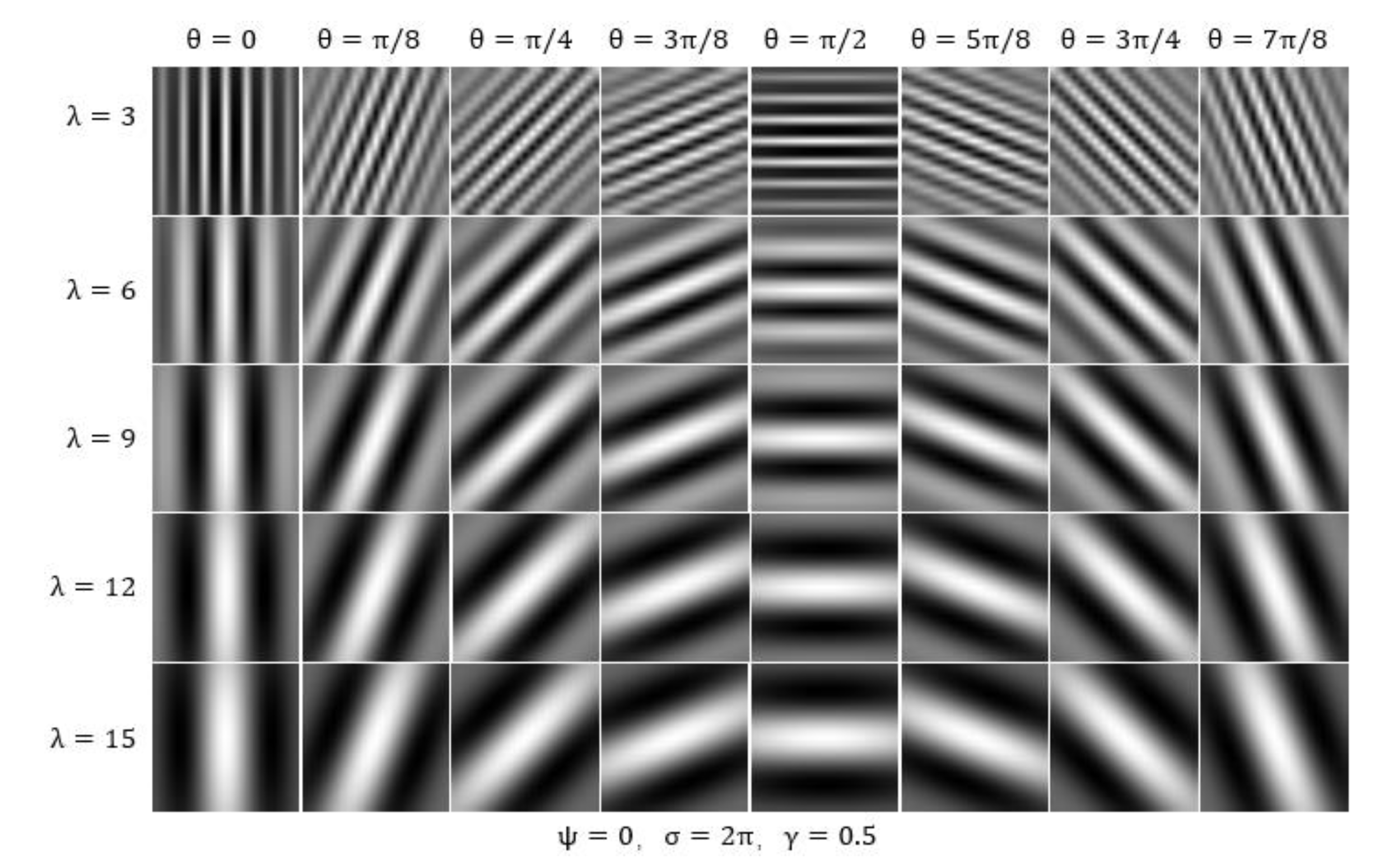
Figure 3.
Example Images of Features Classification (Images processed by authors as fair use from wikiart.org).
Figure 3.
Example Images of Features Classification (Images processed by authors as fair use from wikiart.org).
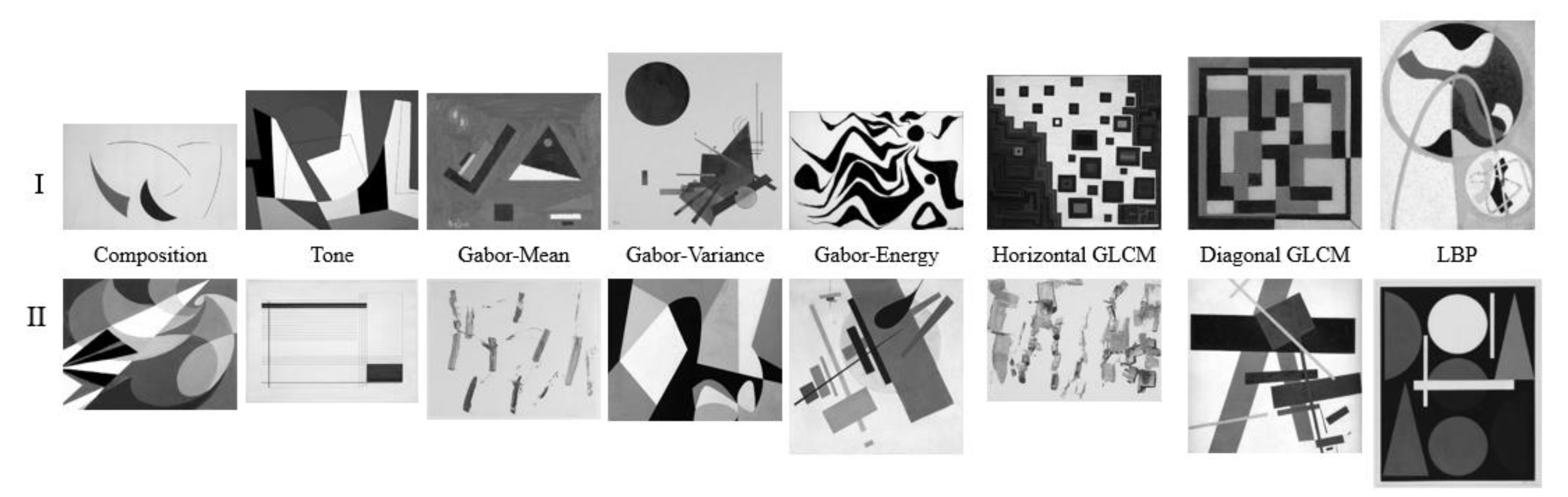
Figure 4.
Illustration of the stimulus paradigm applied.
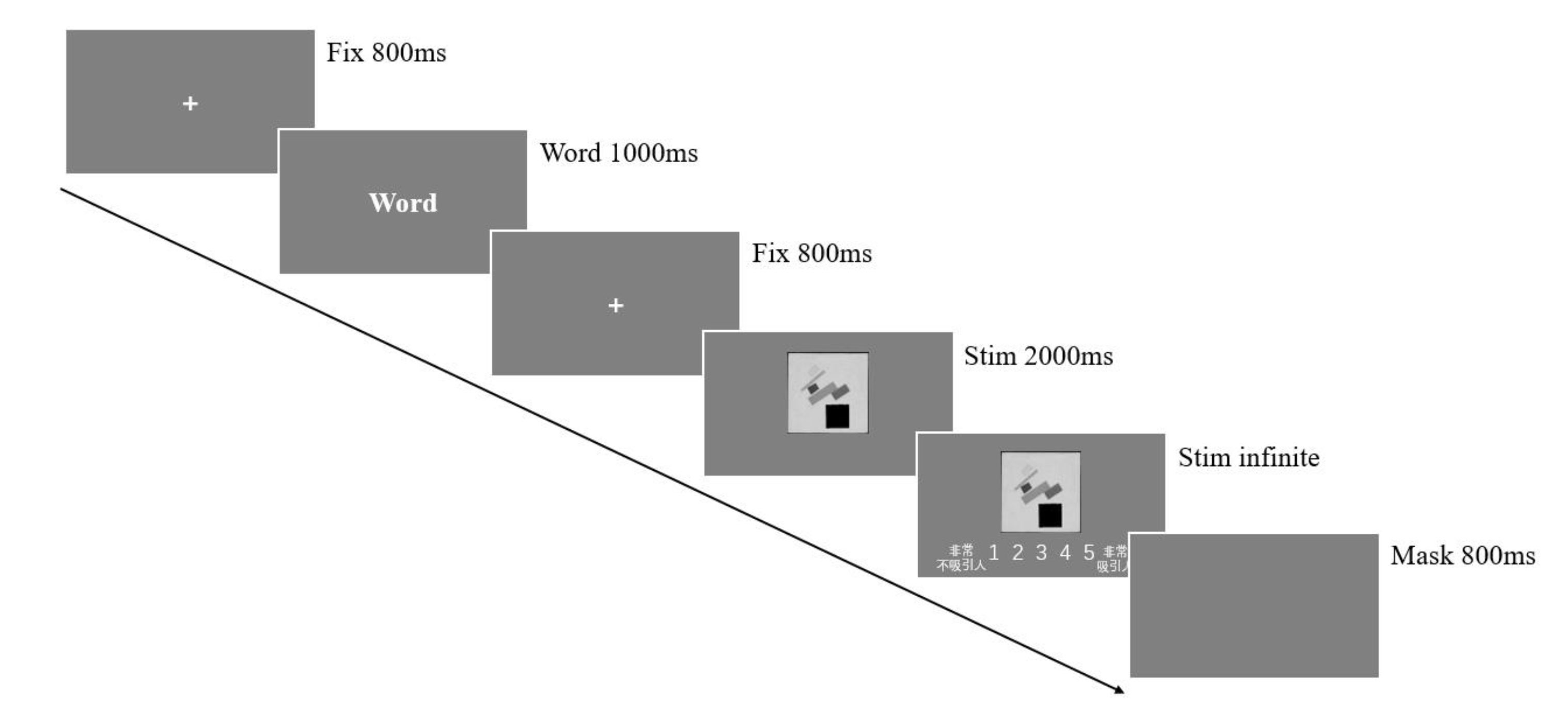
Figure 5.
Grand-average event-related brain potentials and isopotential contour plot for genuine and fake context. N=12.
Figure 5.
Grand-average event-related brain potentials and isopotential contour plot for genuine and fake context. N=12.
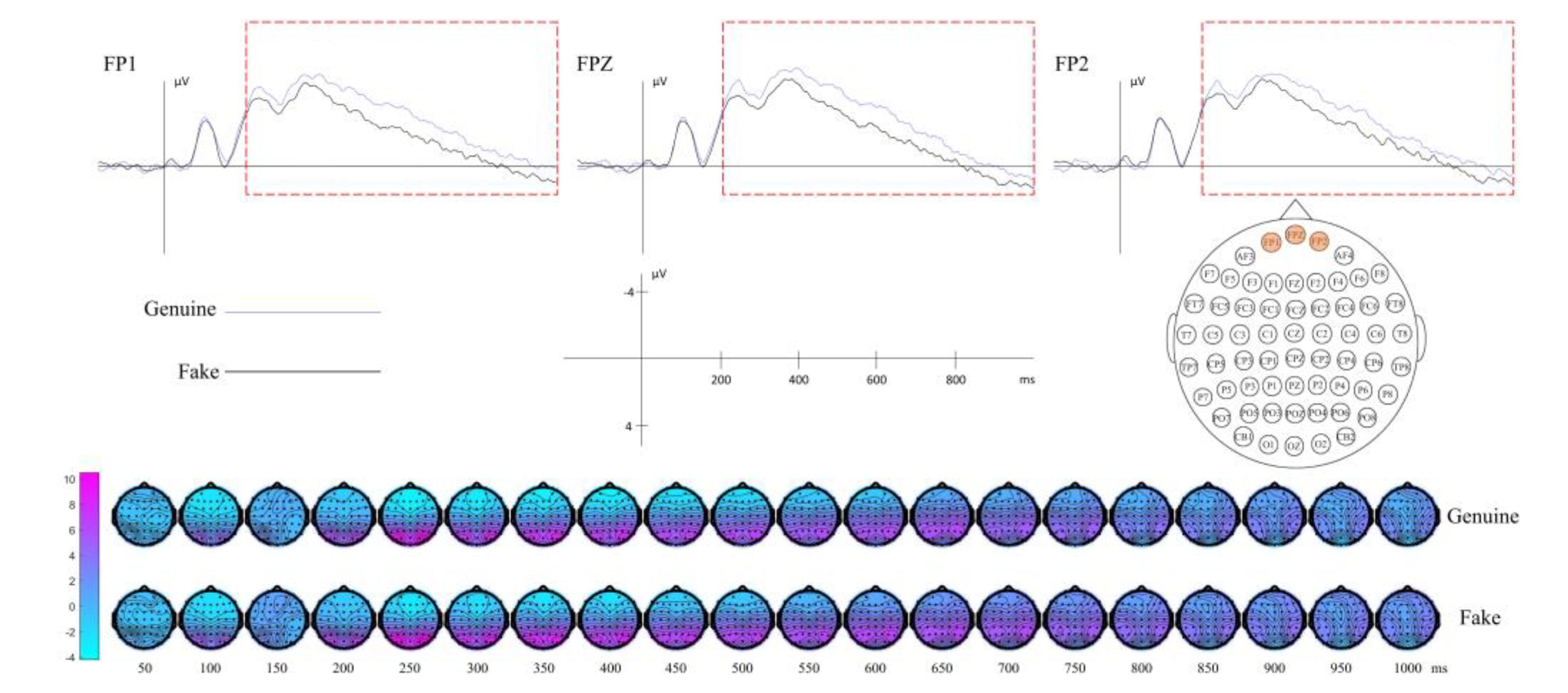
Figure 6.
Grand-average event-related brain potentials and isopotential contour plot for context (genuine, fake) × composition (Class I, Class II). N=12.
Figure 6.
Grand-average event-related brain potentials and isopotential contour plot for context (genuine, fake) × composition (Class I, Class II). N=12.
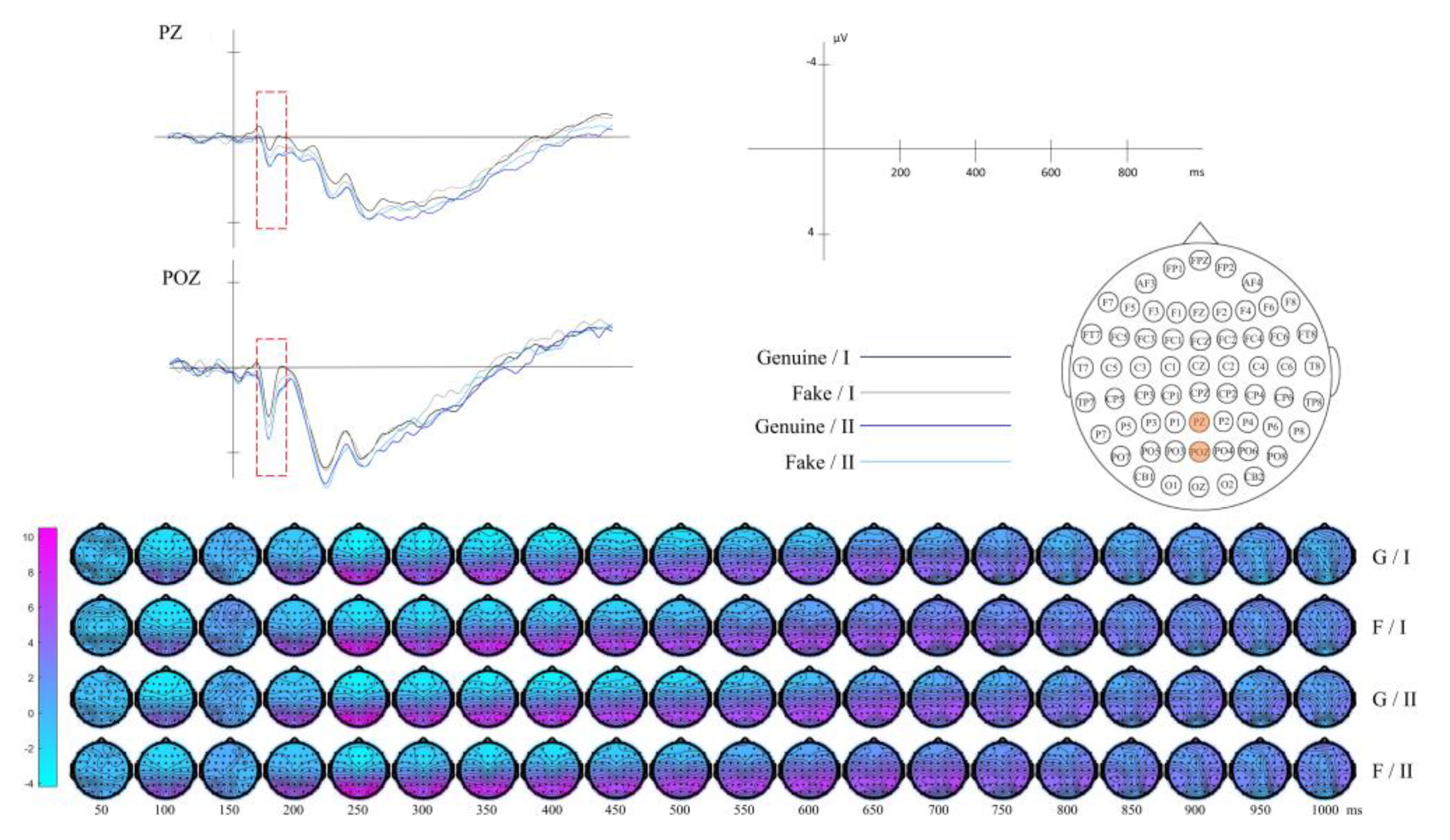
Figure 7.
Grand-average event-related brain potentials and isopotential contour plot for context (genuine, fake) × tone (Class I, Class II). N=12.
Figure 7.
Grand-average event-related brain potentials and isopotential contour plot for context (genuine, fake) × tone (Class I, Class II). N=12.

Figure 8.
Grand-average event-related brain potentials and isopotential contour plot for context (genuine, fake) × Gabor-Mean (Class I, Class II). N=12.
Figure 8.
Grand-average event-related brain potentials and isopotential contour plot for context (genuine, fake) × Gabor-Mean (Class I, Class II). N=12.
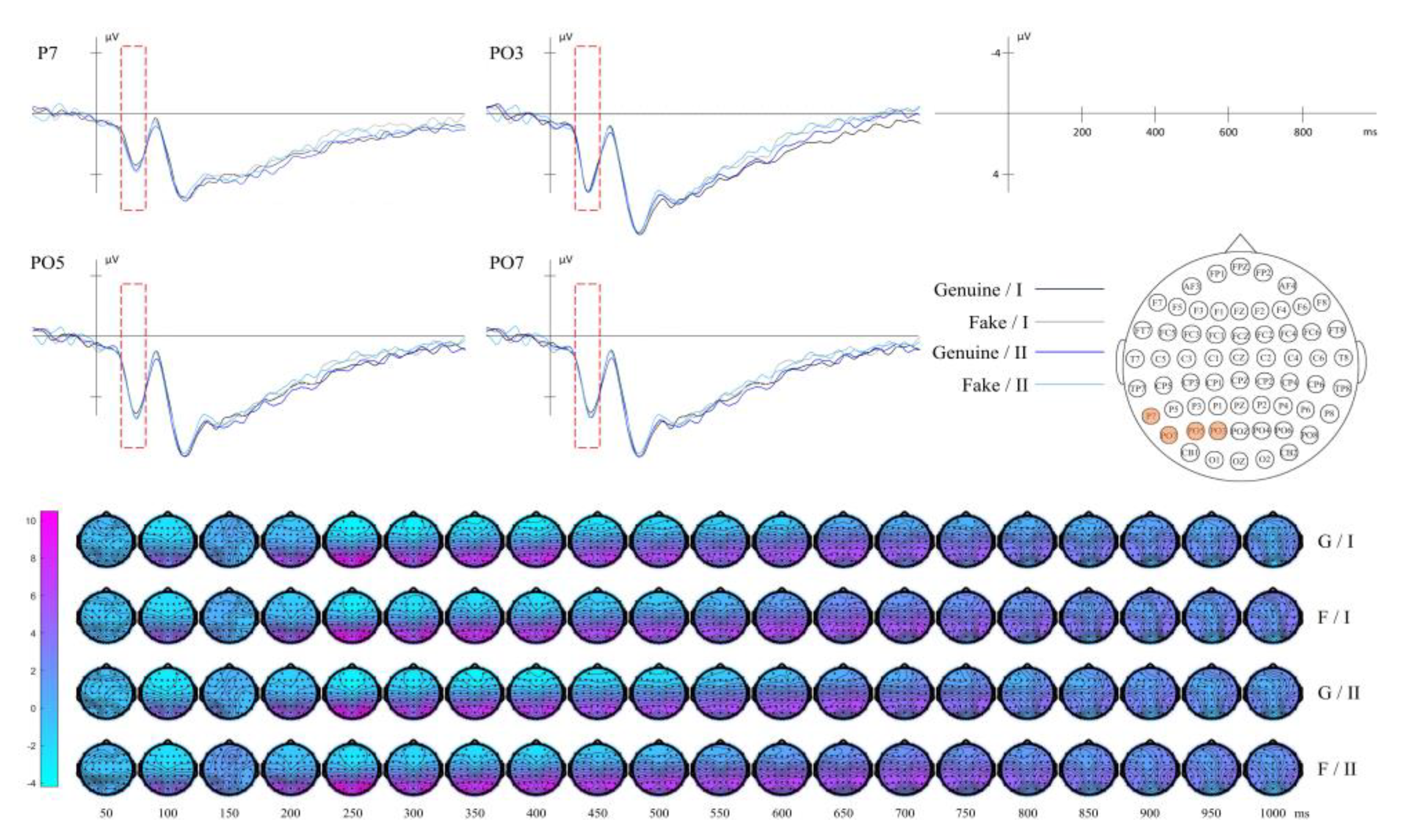
Figure 9.
Grand-average event-related brain potentials and isopotential contour plot for context (genuine, fake) × Gabor-Variance (Class I, Class II). N=12.
Figure 9.
Grand-average event-related brain potentials and isopotential contour plot for context (genuine, fake) × Gabor-Variance (Class I, Class II). N=12.
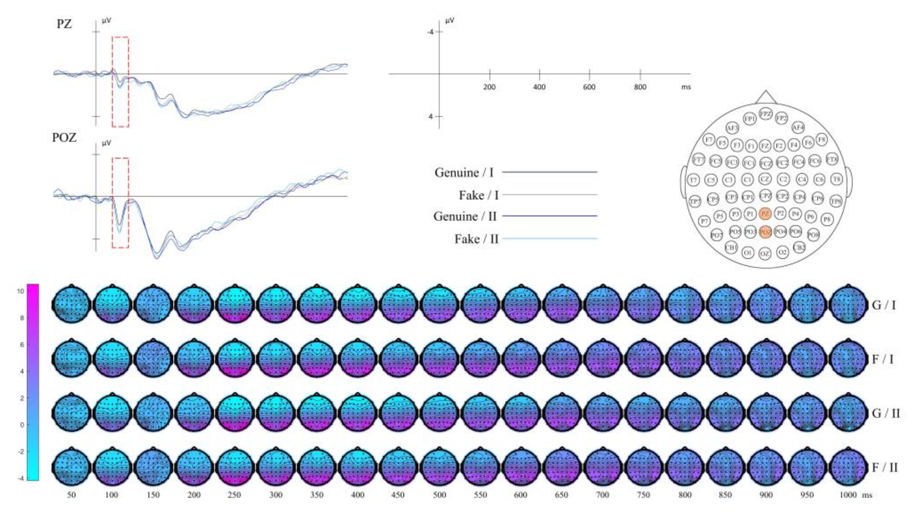
Figure 10.
Grand-average event-related brain potentials and isopotential contour plot for context (genuine, fake) × Gabor-Energy (Class I, Class II). N=12.
Figure 10.
Grand-average event-related brain potentials and isopotential contour plot for context (genuine, fake) × Gabor-Energy (Class I, Class II). N=12.
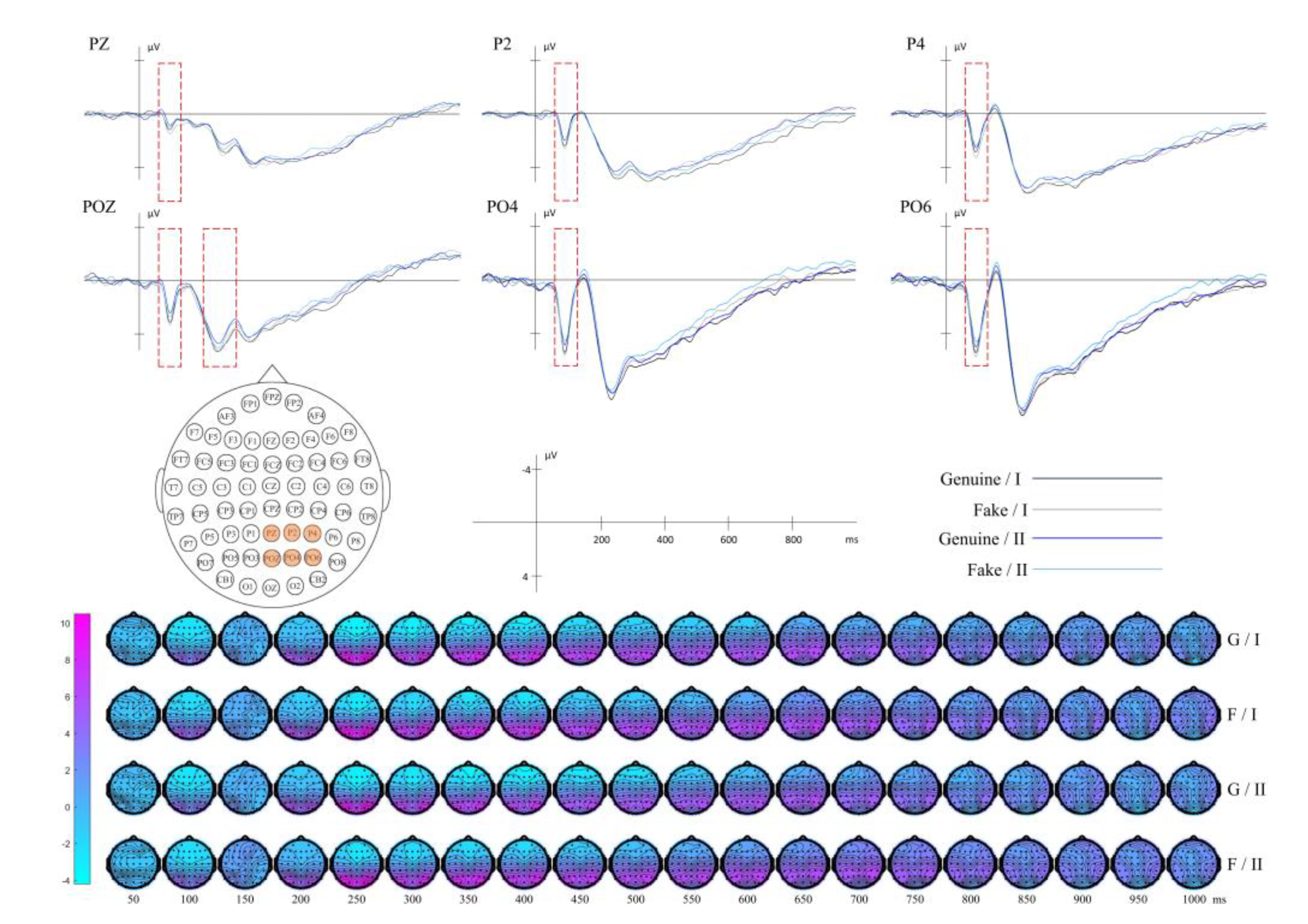
Figure 11.
Grand-average event-related brain potentials and isopotential contour plot for context (genuine, fake) × horizontal GLCM (Class I, Class II). N=12.
Figure 11.
Grand-average event-related brain potentials and isopotential contour plot for context (genuine, fake) × horizontal GLCM (Class I, Class II). N=12.
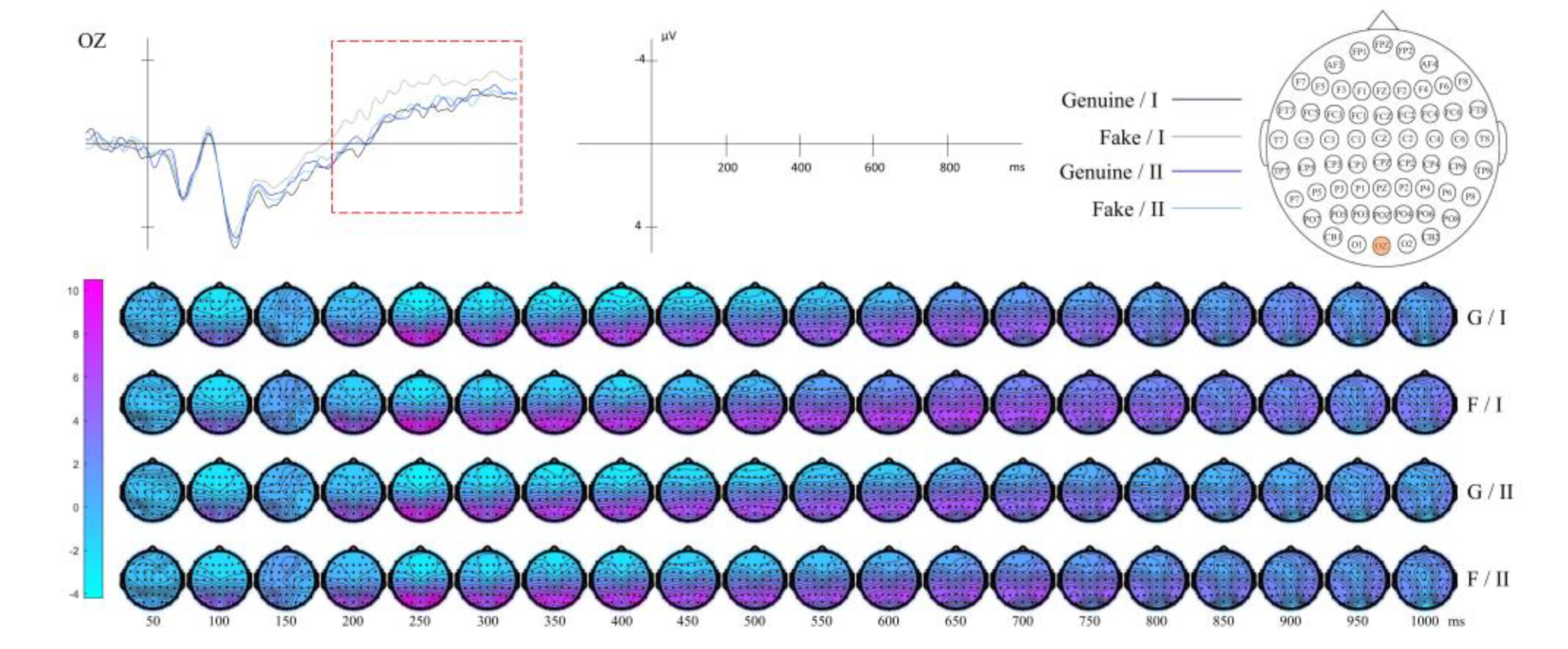
Figure 12.
Grand-average event-related brain potentials and isopotential contour plot for context (genuine, fake) × diagonal GLCM (Class I, Class II). N=12.
Figure 12.
Grand-average event-related brain potentials and isopotential contour plot for context (genuine, fake) × diagonal GLCM (Class I, Class II). N=12.
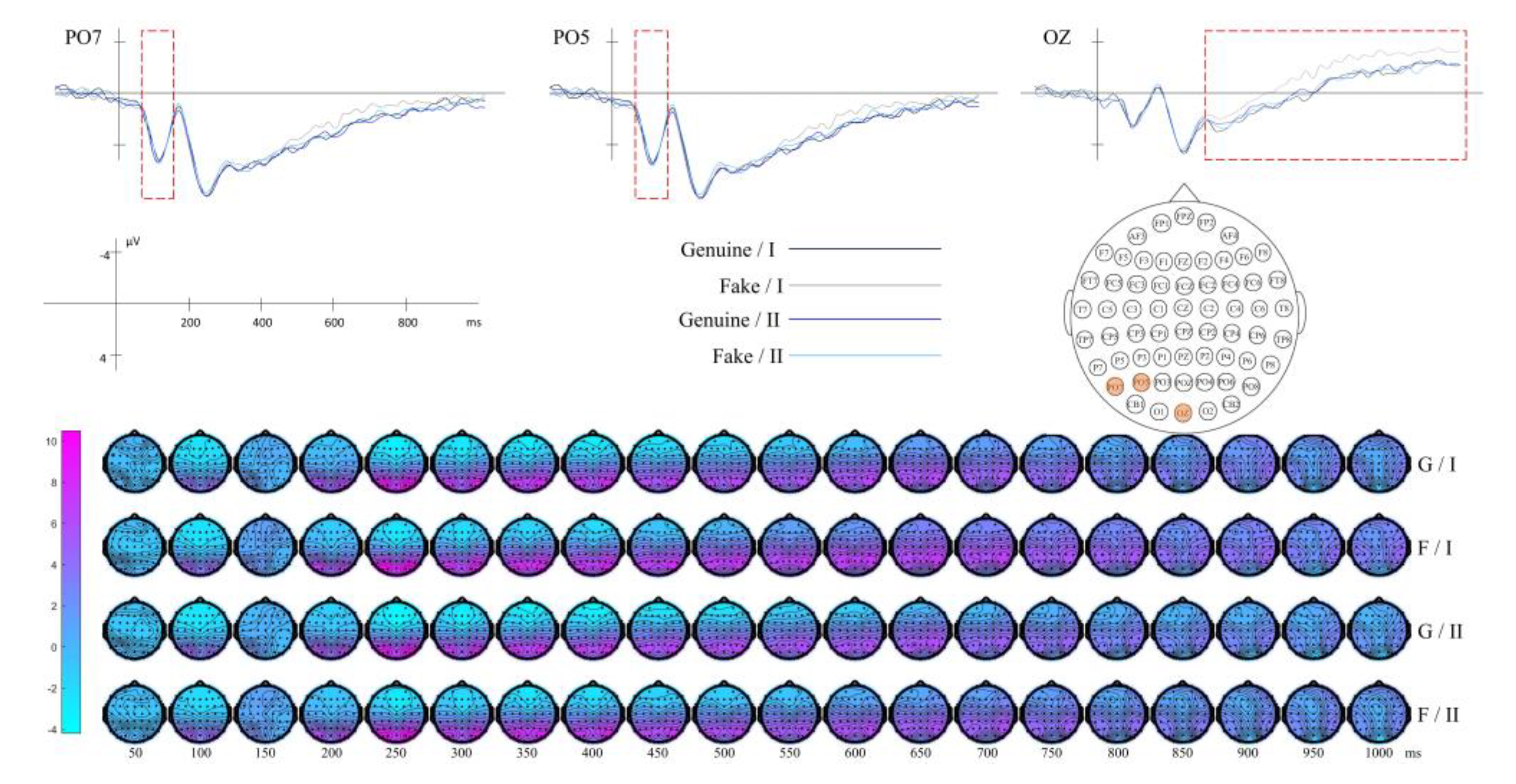
Figure 13.
Grand-average event-related brain potentials and isopotential contour plot for context (genuine, fake) × LBP (Class I, Class II). N=12.
Figure 13.
Grand-average event-related brain potentials and isopotential contour plot for context (genuine, fake) × LBP (Class I, Class II). N=12.
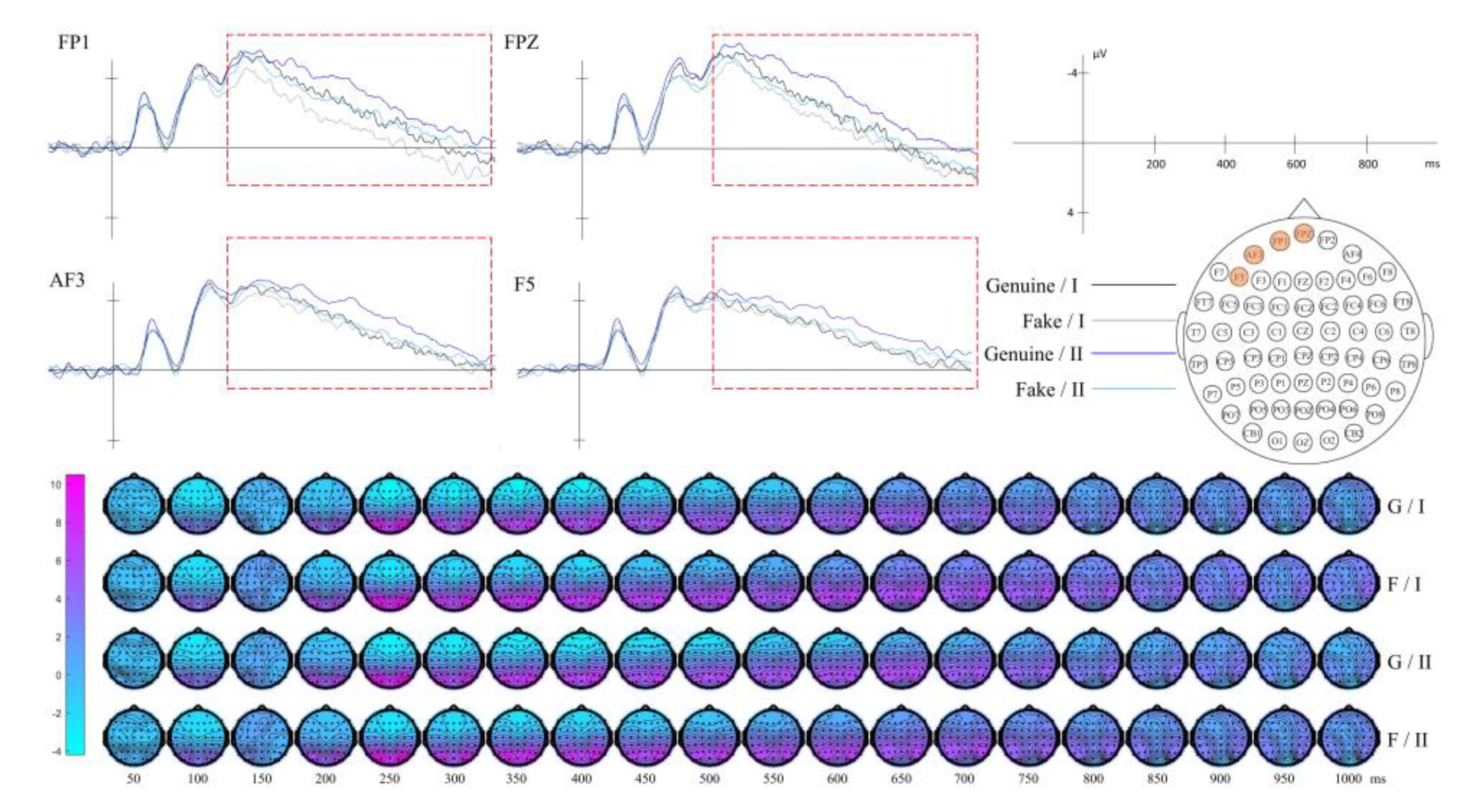
Figure 14.
Performance of SVM Models with Varying C and γ Values: (a) The ACC with Different C and γ Combinations; (b) The AUC with Different C and γ Combinations.
Figure 14.
Performance of SVM Models with Varying C and γ Values: (a) The ACC with Different C and γ Combinations; (b) The AUC with Different C and γ Combinations.
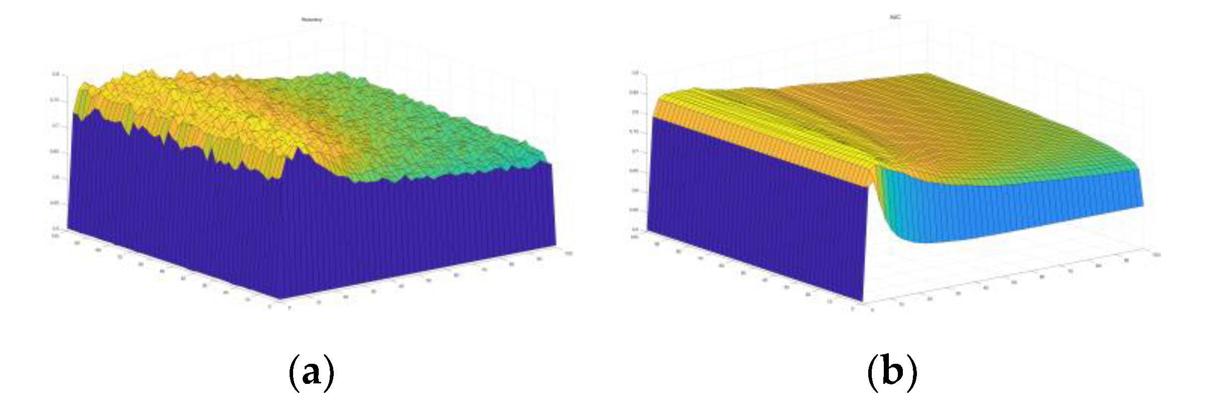
Table 1.
Image Features Classification and Description.
| Features | Class | N | Description |
|---|---|---|---|
| Composition | I | 123 | Class I has a larger blank area compared to Class II. |
| II | 126 | ||
| Tone | I | 105 | The average brightness of Class I is lower than that of Class II, and the gray-level distribution is more discrete. |
| II | 144 | ||
| Gabor-Mean | I | 117 | In the following combinations - (6, 0), (6, π/2), (9, π/8), (9, 3π/8), (9, 5π/8), (9,7π/8), (12,0), (12, π/8) , (12, 3π/8), (12, π/2), (12, 5π/8), (12, 7π/8), (15,0) , (15, π/2) , the grayscale mean of the filtered images in Class I is higher than that of Class II. This indicates that Class I has a higher overall brightness in these combinations. Conversely, Class II exhibits more high-brightness features in other combinations. |
| II | 132 | ||
| Gabor-Variance | I | 130 | In all the combinations, Class II has more high-frequency components and greater texture changes after Gabor filter processing, which suggests that it contains more diverse and complex textures. |
| II | 119 | ||
| Gabor-Energy | I | 122 | In the following combinations - (6, 0), (6, π/2), (9, π/8), (9, 3π/8), (9, 5π/8), (9,7π/8), (12,0), (12, π/8) , (12, 3π/8), (12, π/2), (12, 5π/8), (12, 7π/8), (15,0) , (15, π/2) - the energy gray level of Class I after Gabor filter processing is greater. The features in Class I are more pronounced and intense, likely containing more edges, lines, or texture features in these combinations. Conversely, Class II contains more prominent edges or complex textures in other combinations. |
| II | 127 | ||
| Horizontal GLCM (θ=0°) | I | 123 | In the horizontal direction, compared to Class II, the texture features of Class I are more obvious, with high-contrast edges and lines, higher regularity, and more texture patterns. |
| II | 126 | ||
| Diagonal GLCM (θ=135°) | I | 118 | In the diagonal direction, compared to Class II, the texture features of Class I are more obvious, with high-contrast edges and lines, higher regularity, and more texture patterns. |
| II | 131 | ||
| LBP | I | 113 | Compared to Class II, Class I has weaker texture contrast, but richer details, uniform texture distribution, and contains more small and intense details. |
| II | 136 |
Table 2.
Details of Input and Output Layer Data.
| Input Layer | Output Layer | |||
|---|---|---|---|---|
| Context and Features | Average amplitude of ERP / μV | |||
| Channel | Time Window / ms | |||
| Context | Genuine/Fake | FP1, FPZ, FP2 | 200-1000 | Aesthetic Evaluation |
| Composition | Blank Space | PZ, POZ | 50-120 | |
| Tone | Gray Histogram | OZ | 200-300 | |
| Global Texture | Gabor-Mean | P7, PO3, PO5, PO7 | 70-130 | |
| Gabor-Variance | PZ, POZ | 70-130 | ||
| Gabor-Energy | P2, P4, PZ, PO4, PO6, POZ | 70-130 | ||
| Local Texture | Horizontal GLCM | OZ | 500-1000 | |
| Diagonal GLCM | PO5, PO7 | 70-140 | ||
| OZ | 300-1000 | |||
| LBP | AF3, P5, FP1, FPZ | 300-1000 | ||
Table 3.
Models with best combinations of C and γ.
| Metrics | Values | |
|---|---|---|
| Best C | 28.5786 | |
| Best γ | 14.2943 | |
| Train ACC | 0.79801 | |
| Test ACC | 0.76866 | |
| AUC | 0.74155 | |
| Precision | 0.78241 | 0.75269 |
| Recall | 0.78605 | 0.74866 |
| F1 | 0.78422 | 0.75067 |
Disclaimer/Publisher’s Note: The statements, opinions and data contained in all publications are solely those of the individual author(s) and contributor(s) and not of MDPI and/or the editor(s). MDPI and/or the editor(s) disclaim responsibility for any injury to people or property resulting from any ideas, methods, instructions or products referred to in the content. |
© 2024 by the authors. Licensee MDPI, Basel, Switzerland. This article is an open access article distributed under the terms and conditions of the Creative Commons Attribution (CC BY) license (http://creativecommons.org/licenses/by/4.0/).
Copyright: This open access article is published under a Creative Commons CC BY 4.0 license, which permit the free download, distribution, and reuse, provided that the author and preprint are cited in any reuse.


