Submitted:
27 March 2025
Posted:
27 March 2025
You are already at the latest version
Abstract
The standard chi-square test, developed by Pearson (1900) determines whether significant differences exist between frequencies of data categories, each containing unique subjects. In other words, each subject provides data for only one category. This stipulation prevents analysis of longitudinal data pertaining to subjects’ categorization at more than one point in time. The McNemar test (1947) produces a chi-square value that, in contrast to the Pearson chi-square value, accounts for dichotomous data from a single sample measured twice. Although extremely beneficial for data analysis, the McNemar test cannot be used for situations involving more than two measurements of the sample. This article, therefore, establishes a formula to compare dichotomous data from three or more trials involving the same subjects. An example demonstrates the formula’s applicability in a three-trial situation. Further expansion of the formula used for this example, as described in subsequent text, makes it possible to evaluate differences in repeated-measures frequencies for any number of trials.
Keywords:
chi-square test
; categorical analysis
; repeated measures
; longitudinal analysis
; McNemar test
1. Introduction
Measurement of categorical variables often seems relatively simple. Descriptive statistics pertaining to categorical data are limited to frequencies, proportions, and, in the case of ordered categories, percentiles. These values, when pertaining to univariate analyses, appear in a frequency table, bar graph, or pie chart. For multivariate analyses, data generally appear in a crosstabulation, clustered bar graph, or stacked bar graph. Inferential statistical tests for categorical data rest upon hypotheses suggesting relationships between category frequencies.
In the univariate context, research hypotheses usually predict inequalities between category frequencies or combination of category frequencies. The corresponding null hypotheses either predict equality between all category frequencies or between one combination of category frequencies and another combination of category frequencies. Evaluating these sorts of hypotheses requires the use of Pearson’s non-parametric chi-square (test [1], shown as Equation 1. In this formula, represents the observed frequency and represents the expected frequency for each category (i) in a frequency table or crosstabulation.
Although this equation effectively tests for significant difference, or heterogeneity, it does so only under the assumption of unique subjects in each category. The chi-square test does not apply to a situation involving data obtained from a single set of subjects measured multiple times. As plainly stated by McHugh [2] (p. 144), “The study groups must be independent. This means that a different test must be used if the two groups are related.”
Equation 1 could be used, for example, to compare frequencies of people who do and do not have blood pressure. This evaluation would compare frequencies for the with high blood pressure (at least 130/80 [3]) and for the group without high blood pressure at a single point in time. However, an evaluation of whether group membership changes longitudinally, with data gathered at multiple points in time, could not use this formula. For example, one who wishes to determine whether individuals have high blood pressure before, during, and after watching a horror movie may test a single set of subjects at three distinct points in time. A standard Pearson chi-square test could not evaluate the significance of differences between cell frequencies because the same subjects provide data for each trial, represented as column in Table 1.
Because the subjects repeat the trial, in this case a blood pressure test, some use phrases such as “paired samples” [2] (p. 144), [4,5] (p. 1193) and “repeated measures” [6,7]to describe this type of design. These phrases reflect the terminology used to evaluate differences in means of a single subject group tested twice, as a paired-samples t-test does, or more than two times, as a repeated-measures or within-subjects ANOVA does. For data in a crosstabulation, however, analyses focus upon significant differences between frequencies, not between means. A chi-square test, rather than a t-test or an ANOVA would be used. Specifying that this chi-square test uses paired samples or repeated measures indicates the reuse of subjects in independent-variable trials.
In 1947, McNemar [8] developed a test to evaluate significant differences in category frequencies of a dichotomous variable in a repeated sample. Using a 2x2 Punnett square or contingency table approach, McNemar (arranged data from two trials, T1 and T2, each with a dichotomous option, such as “yes” and “no,” as shown in Figure 1.
The McNemar test focuses upon subjects whose scores or responses change between the first and the second trial, namely Figure 1’s A and D. Cells that indicate no change (B + C) received a weight of 0 and, consequently, do not impact calculations of McNemar’s chi-square value. Using the arrangement of A and D shown in Equation 2, the McNemar chi-square formula (acknowledges that the same subjects provided data for trial 1 and trial 2 [8].
As the formula suggests, McNemar’s chi-square can only account for two conditions and with only two groups of subjects in each condition. It could not accommodate the longitudinal study that compares frequencies from “before,” “during,” and “after” trials, described earlier. Cochran’s Q test [9], often considered an expansion of McNemar’s test, allows for the consideration of repeated measures across more than two trials. Although reasonably well-accepted, some [10,11,12,13] have noted that the Q statistic can easily become unwieldy to calculate and challenging to use. Further, the distribution of Q can vary according to the estimated value of a nuisance variable [10] and, possibly most importantly, “Cochran deliberately did not use Q itself to test for heterogeneity.” [14] (p. 485).
A different approach to expanding McNemar’s formula can compare three of more longitudinal frequencies relatively succinctly. This expansion begins by considering the standard McNemar test formula and the logic behind it.
2. Methods
The first step in expanding this test to account for a longitudinal study with more than two trials involves converting the Punnett square into a Punnett cube based upon T1, T3 , and T3. With respect to the blood pressure example, T1 would refer to the “before” trial, T2 would refer to the “during” trial, and T3 would refer to the “after” trial.
Figure 2 provides the information needed to identify the frequencies or percentages for all combinations of category frequencies. However, identifying particular values can become challenging due to the complexity of the three-dimensional representation. Restructuring it into the three two-dimensional representations, as shown in Figure 3, helps to clarify the changes that occur between trials. Although the two squares on the top of the illustration use the arrangement of “yes” and “no” options in Figure 2, the other uses reversed positioning of the options for Trial 3. This adjustment does not change the structure of the data, but merely repositions the values so that they appear consistent with the arrangements in the top two squares. This representation makes the combination of “yes” and “no” frequencies each pair of trials evident.
As with McNemar’s method, cells corresponding to changed responses, become relevant to this analysis. Following his practice of adding together frequencies of cells as he does with Figure 1’s B and C), grouping together corresponding cells from the squares in Figure 3 produces the schema shown in Table 2.
3. Results
Rather than simply referring to A and D, as McNemar’s formula does, the formula that accounts for a third trial refers to (A+E+I) and (D+H+L). The “R” subscript in Equation 3 denotes the test’s applicability for the repeated measures condition.
Within a dichotomous trial, 1 degree of freedom (df) exists due to the standard of subtracting 1 from the number of categories (2-1=1). Acknowledgement of multiple trials, as in the scenario addressed in this article, also follows the precedent [12,13,15] of incorporating K-1, with K indicating the number of trials, into the df formula. When multiplied by the value of 1, representing variation between dichotomous options within each individual trial, the overall formula becomes
df = (1)(K-1) = K-1 .
Although Figure 3 and Figure 4 and Equation 3 address a scenario involving three trials, this process can accommodate additional trials as well. The discussion portion and Appendix A of this article provide guidance for evaluating repeated-measures frequencies with four or more trials.
With knowledge of the calculated statistic from Equation 3, and the degrees of freedom, from Equation 4, the remainder of the evaluation follows the same procedure that most tests of significance do. The critical value that serves as a comparison factor for the calculated appears at the intersection of the appropriate df row and significance threshold (α) column of a critical value table. A calculated that exceeds the critical value ( indicates significant differences or inconsistencies between frequencies and a critical value that exceeds the calculated value indicates no significant differences or inconsistencies between frequencies.
4. Discussion and Application
A demonstration of this process can use data pertaining to weather trends, as this data is collected both expertly and objectively. Further, the lack of human subject participation eliminates the need for IRB approval. Cornell University’s Northeast Regional Climate Center’s website [16] provides information about temperature departures from normal for various time periods over many years. Data pertaining to the spring months (March, April, and May) of 2021, 2022, and 2023 appears in Appendix B. These values indicate the difference, in degrees Fahrenheit (F), between mean spring temperatures in these years and the normal spring temperatures (the mean from 1991-2000), in 54 northeastern U.S locations.
Suppose a researcher, perhaps investigating the issue of global warming, divides the departure values into two categories: those indicating temperatures greater than 1o above normal and those indicating temperatures not greater than 1o above normal. A “yes” (greater than 1o above normal) and “no” (not greater than 1o above normal), then exists for 2021, for 2022, and for 2023, labeled T1, T2, and T3, respectively. With awareness that 2023 has been deemed the warmest year in recent history [17], the researcher might reasonably hypothesize that the frequency for T3’s “yes” category exceeds the frequency of any other category involved in the analysis. A multi-part research hypothesis most simply represents this assertion.
The null hypothesis that corresponds to this research hypothesis (and to any research hypothesis based upon the “yes” and “no” frequencies for the three years considered) states.
The Punnett cube in Figure 4 displays frequencies for each combination of “yes” and “no” categories among the three years examined.
Figure 5 displays frequencies for the associated 2x2 Punnett squares. It is important to realize that values in these squares often exceed the values in Figure 4 because the cube imposes an additional restriction (e.g. a third variable’s outcome) upon each frequency.
To test the null hypothesis, calculations based upon Equation 3 take the following form.
The last step of the process involves comparing the calculated value () obtained from Equation 5 to the critical value () obtained from a chi-square critical value table. Obtaining the second of these values requires knowledge of the degrees of freedom and the determination of α, which represents the maximum probability of incorrectly claiming that a significant difference between frequencies exists. In this case, df = 3-1 = 2 based upon Equation 4. Although researchers have some liberty when selecting the α value, this example uses the standard of 0.05.
With 2 degrees of freedom and α = .05, = 5.99. This value does not exceed the calculated of 6.74, indicating less than 95% level of certainty of a significant difference between frequencies in Figure 4, thus supporting the null hypothesis. Had the results indicated a significant difference, then analysis would continue. Post-hoc testing to determine whether this T3 “no” category frequency drives the significance could begin by comparing values in Figure 5’s individual Punnett squares using the traditional McNemar test.
5. Conclusions
The use of rather than values from multiple McNemar tests rests upon the same logic as the use of an ANOVA rather than multiple t-tests does. For a variable that encompasses more than two groups or trials, comparing two frequencies at a time increases the probability of making a Type 1 error in the overall analysis [18]. Like an ANOVA, Equation 3 provides a comprehensive evaluation of data with a single analysis while minimizing the probability of incorrectly claiming that a significant difference exists.
Cochran’s Q test also indicates the presence or absence of a significant difference among repeated-measures frequencies, but it does so in a different way than the test described in this article does. In addition to involving a complex formula, Cochran’s Q test rests upon the assumption of at least 24 subjects and frequencies greater than three in divergent (e.g. yes/no and no/yes) categories. This assumption does not apply to the McNemar test [12] making it an appropriate basis for establishing a test to evaluate data sets with small category frequencies, such as those in this article’s example.
5.1. Further Uses for the Equation
Preceding sections describe and exemplify the process of comparing frequencies across three trials with repeated subjects. Slight adjustments to Equation 3, however, broaden its applicability. For example, some crosstabulation cells contain percentages rather than frequencies. Additionally, studies may involve more than three trials. The structure of Equation 3 can accommodate both of these situations.
Because obtaining percentage values simply requires dividing frequencies by N, the relationships between frequencies and their corresponding percentages in a crosstabulation is identical. Equation 3, therefore, produces the same value regardless of whether A, E, I, D, H, and L represent frequencies or percentages.
The formula can also accommodate as many cell frequencies or percentages as needed to address the number of trials conducted. Visually representing four or more trials becomes somewhat challenging due to the inability to draw more than that three dimensions of a Punnett cube on a two-dimensional surface (paper). One must resort to either nesting trials within a single cube or using more than one cube. Sample diagrams, applicable to four trials, appear in Appendix A. Each additional trial (t) increases the number of Punnett squares by (t-1) beginning with the three squares used for a three-trial case. So, the arrangement for an analysis with four trials would use six [3+(4-1)] squares, the arrangement for an analysis with five trials would use ten [6+(5-1)] squares, an arrangement for an analysis with six trials would use 15 [10+(6-1)] squares, and so on. But, the resulting Punnett squares still follow the pattern displayed in Figure 4 and Figure 6. Each displays YN frequencies in the upper left, NN frequencies in the bottom left, YY frequencies in the upper right, and NY frequencies in the bottom right. An analysis with more than four trials cannot use the same notation as that used in Figure 5, only because the alphabet does not contain enough letters to uniquely identify each condition. Numbering the squares and using corresponding subscripts for the letters A, B, C, and D, however, allows for the expansion of Equation 3 to accommodate any number of trials. Calculation of degrees of freedom for this expanded test uses Equation 4.
5.2. Limitations
Limitations of the McNemar test and, in some cases, the chi-square test, also apply to the test described in this article. Many of these issues pertain to sample size and category frequencies.
McNemar [8], himself, noted that his formula should be used only if (A+D) 10. With small samples, the test has low power due to inflated p values [19]. This limitation also applies to the use of Equation 3 and Equation 6 and, therefore, those using these equations to evaluate small data sets may wish to set the α value slightly higher than they normally would.
With respect to the standard chi-square test, McHugh [2] (p. 143) described the “difficulty of interpretation when there are large numbers of categories (20 or more) in the independent or dependent variable.” Thus, although Equation 6 has the potential to evaluate data from an infinite number of trials, those using it to test hypotheses involving many categories should take caution.
5.3. Final Points
This repeated measures chi-square test presented in this article differs from the standard chi-square and McNemar’s chi-square in subtle yet important ways. The standard chi-square test can evaluate data from an infinite number of variables as long as all categories in the analysis are mutually exclusive. McNemar’s test applies to situations with repeated measures, but does so only for two trials of a dichotomous variable. The presented test, however, allows for repeated measures as well as more than two trials. Figure 6 provides a representation of this relationship.
Although the use of the term “trials” in this article to distinguish between multiple independent-variable measures may imply lapses in time, time does not necessarily need to be the distinguishing factor between measures. Distinguishing factors can pertain to place, circumstances, presence of particular stimuli, and many other variations.
The repeated measures chi-square test’s suitability for situations that neither the standard nor the McNemar chi-square test can address prompts curiosity about whether another test can expand upon the McNemar test in a different way. In addition to requiring only two trials, the McNemar test can only address situations with dichotomous independent variables. Developing a variation of the test that can evaluate differences in frequencies of non-dichotomous variables, perhaps with “yes,” “unsure,” and “no” options, within a repeated-measures context would further broaden statistical capabilities. Although the Stuart-Maxwell test [20,21] can evaluate significant differences in a kxk repeated-measures scenario [22], it cannot evaluate significance if the numbers of categories and trials differ. Visual representations would, thus, not resemble Punnett square, with diverging results shown along diagonals. The main challenge in developing a test that does so lies with determining how to structure the numerator of the chi-square formula given more than two expressions of divergent outcomes. Such a formula, however, would make it possible to evaluate differences between any number of variable categories across any number of repeated-measures trials, serving a yet unmet need in the realm of categorical data analysis.
Funding
This research received no external funding
Data Availability Statement
Please see Appendix B for raw data and information about its origin.
Conflicts of Interest
The author declares no conflicts of interest.
Appendix A
Data for an analysis using more than three trials can be arranged in multiple Punnett cubes or in a nested single Punnett cube. Figure A1 and Figure A2, respectively, show these arrangements based upon four trials.
Figure A1.
Multiple Punnett cubes. Separate cubes present the Trial 1 “yes” condition and the Trial 1 “no” condition with each cube containing data for Trial 2, Trial 3, and Trial 4. An analysis involving more than four trials would use additional cubes as needed.
Figure A1.
Multiple Punnett cubes. Separate cubes present the Trial 1 “yes” condition and the Trial 1 “no” condition with each cube containing data for Trial 2, Trial 3, and Trial 4. An analysis involving more than four trials would use additional cubes as needed.
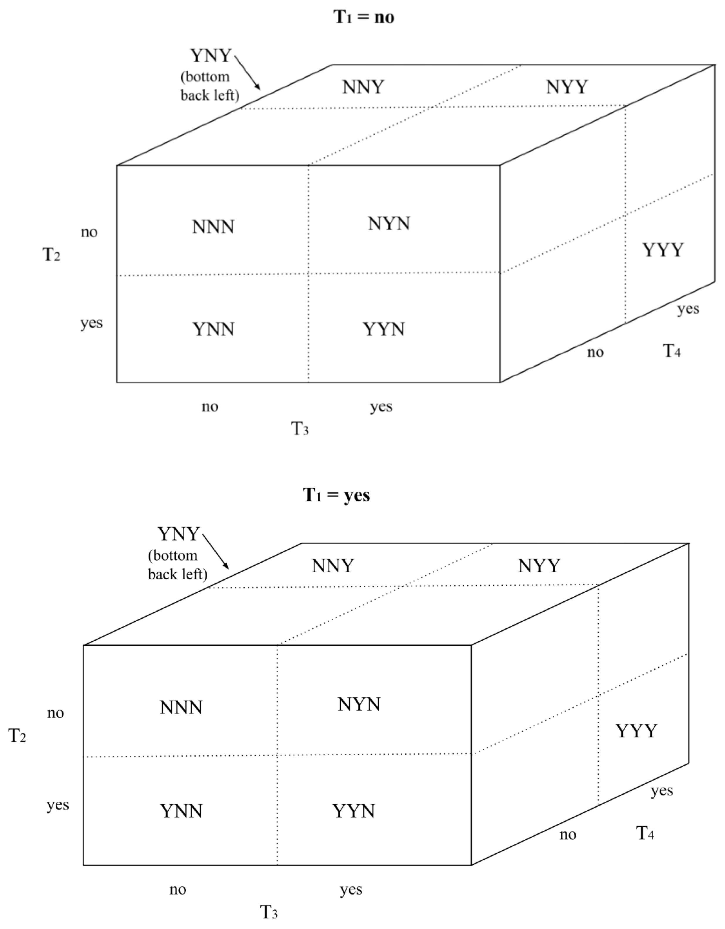
Figure A2.
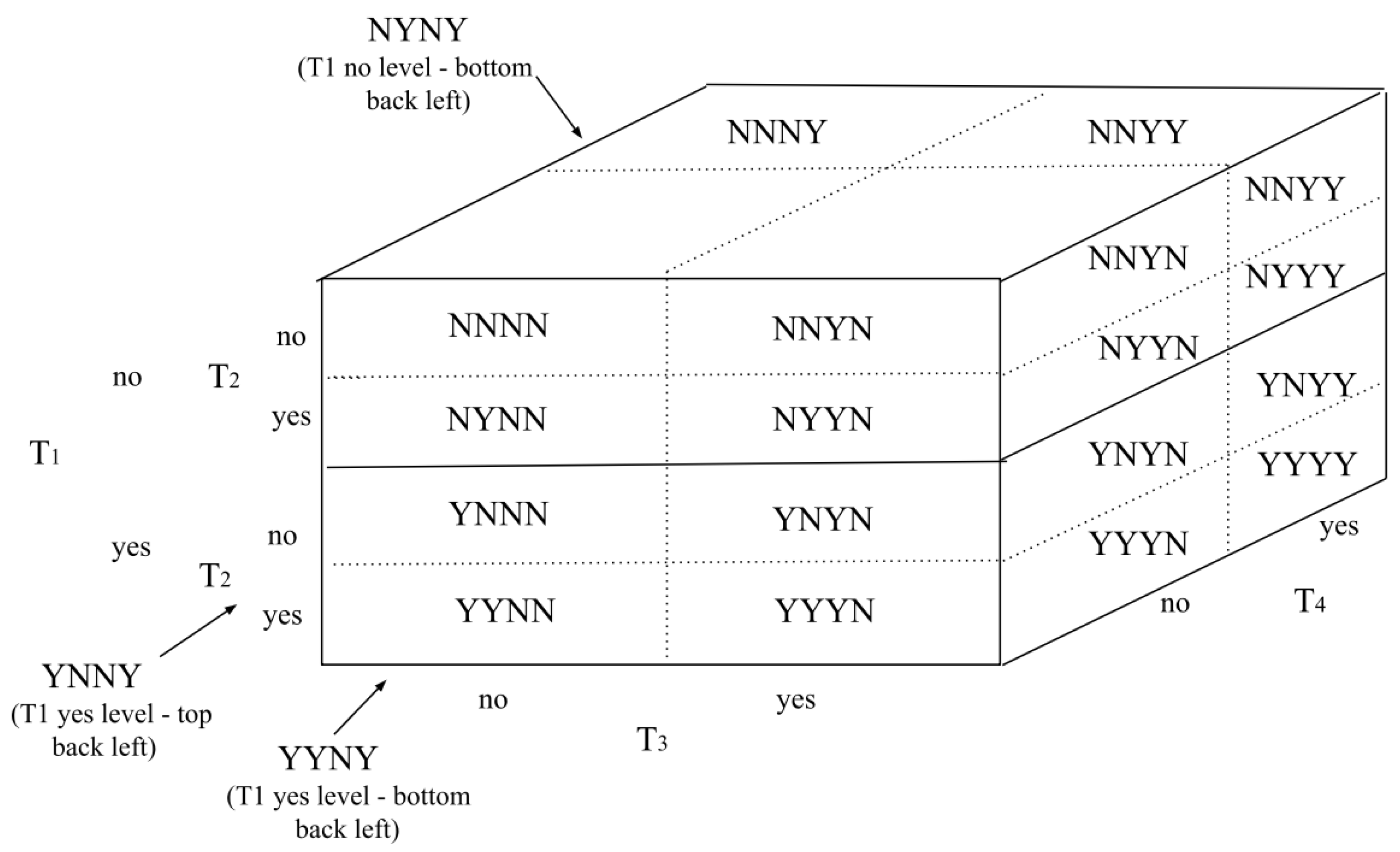
Nested Punnett Cube. The Punnett cube displays Trial 2 categories nested within Trial 1. An analysis involving more than four trials would require additional nesting of categories.
Figure A2.
Nested Punnett Cube. The Punnett cube displays Trial 2 categories nested within Trial 1. An analysis involving more than four trials would require additional nesting of categories.
Appendix B. Raw Data

Table A1.
Raw Data for Example.
| LOCATION | 2021 | 2022 | 2023 |
| 1 | 1.2 | 1.6 | 1.4 |
| 2 | 1.1 | 1.7 | 1.4 |
| 3 | 0.9 | 1.5 | 1.3 |
| 4 | 1 | 1 | 1.1 |
| 5 | 1.5 | 0.9 | 1 |
| 6 | 2.4 | 2 | 1.9 |
| 7 | 2.4 | 2.1 | 1.8 |
| 8 | 2.2 | 2 | 1.7 |
| 9 | 1.5 | 1.6 | 1.3 |
| 10 | 1.2 | 1 | 1 |
| 11 | 1.1 | 1.3 | 1.1 |
| 12 | 1.1 | 1 | 0.9 |
| 13 | 0.7 | 0.6 | 0.8 |
| 14 | 1.1 | 1 | 0.9 |
| 15 | 0.3 | 0.4 | 0 |
| 16 | 0.8 | 0.9 | 0.3 |
| 17 | 1.7 | 2.1 | 1.7 |
| 18 | 1.4 | 1.7 | 1.3 |
| 19 | 2 | 2.2 | 1.8 |
| 20 | 1.4 | 2.4 | 1.9 |
| 21 | 1.7 | 2.2 | 1.6 |
| 22 | 1.8 | 2 | 1.4 |
| 23 | 1.1 | 1.3 | 0.9 |
| 24 | 1.3 | 1.5 | 1.1 |
| 25 | 1.5 | 1.4 | 1.4 |
| 26 | 1.7 | 1.9 | 1.1 |
| 27 | 0.5 | 1.2 | 0.8 |
| 28 | 1.4 | 1.6 | 1 |
| 29 | 1.1 | 1.3 | 1.4 |
| 30 | 1.2 | 1.6 | 1.4 |
| 31 | 0.9 | 1.4 | 1.1 |
| 32 | 1.7 | 1.6 | 1.2 |
| 33 | 2.3 | 1.8 | 1.4 |
| 34 | 1.8 | 1.9 | 0.9 |
| 35 | 1.5 | 1.8 | 0.9 |
| 36 | 0.9 | 1.2 | 1 |
| 37 | 1 | 1 | 0.8 |
| 38 | 1.3 | 1.2 | 0.9 |
| 39 | 1 | 0.8 | 0.7 |
| 40 | 1 | 1 | 0.8 |
| 41 | 1.2 | 1.3 | 1.1 |
| 42 | 1.2 | 1 | 0.6 |
| 43 | 0.8 | 0.7 | 0.4 |
| 44 | 0.6 | 0.6 | -0.1 |
| 45 | 1.3 | 1.3 | 0.7 |
| 46 | 1.3 | 2 | 1.3 |
| 47 | 1.6 | 2 | 1.2 |
| 48 | 1.6 | 1.9 | 1.4 |
| 49 | 1.7 | 2 | 1.5 |
| 50 | 0.2 | 0.6 | -0.3 |
| 51 | 0.3 | 0.8 | -0.3 |
| 52 | -0.6 | 1 | -0.2 |
| 53 | 0.1 | 1 | -0.2 |
| 54 | -0.5 | 1 | -0.2 |
| 55 | 0.6 | 0.6 | 0.1 |
Values represent departures from normal Farenheit temperatures for 55 locations in the northeastern United States during the Spring (March, April, May) of 2021, 2022 and 2023. Normal temperatures equal the mean temperature between 1991 and 2020. Data originates from [16].
References
- Pearson, K. On the criterion that a given system of deviations from the probable in the case of a correlated system of variables is such that it can be reasonably supposed to have arisen from random sampling. The London, Edinburgh, and Dublin Philosophical Magazine and Journal of Science 1900, 50, 157–175. [Google Scholar] [CrossRef]
- McHugh, M.L. The chi-square test of Independence. Biochemia Medica 2013, 23, 143–149. [Google Scholar] [CrossRef] [PubMed]
- Center for Drug Evaluation and Research. High blood pressure–understanding the silent killer. ; U.S. Food and Drug Administration; Available online: http://www.fda.gov/drugs/special-features/high-blood-pressure-understanding-silent-killer. (accessed on 11 April 2024).
- Sundjaja, J.H.; Shrestha, R.; Krishan, K. McNemar and Mann-Whitney U Tests. In National library of medicine; National Institute of Health; Available online: https://www.ncbi.nlm.nih.gov/books/NBK560699/ (accessed on 14 April 2024).
- Schober, P.; Vetter, T.R. Chi-square tests in medical research. Anesthesia & analgesia 2019, 129, 1193. [Google Scholar]
- Klingenberg, B.; Agresti, A. Multivariate extensions of McNemar’s test. Biometrics 2006, 62, 921–928. [Google Scholar] [CrossRef] [PubMed]
- Singh, V.; Rana, R.K.; Singhal, R. “Analysis of repeated measurement data in the clinical trials.”. Journal of Ayurveda and Integrative Medicine 2013, 4, 77. [Google Scholar] [PubMed]
- McNemar, Q. Note on the sampling error of the difference between correlated proportions or percentages. Psychometrika, 1947, 12, 153–157. [Google Scholar] [CrossRef] [PubMed]
- Cochran, W.G. The comparison of percentages in matched samples. Biometrika 1950, 37, 256–266. [Google Scholar] [CrossRef] [PubMed]
- Kulinskaya, E.; Dollinger, M.B. An accurate test for homogeneity of odds ratios based on Cochran’s Q-statistic 2015. BMC Medical Research Methodology 2015, 15. [Google Scholar] [CrossRef] [PubMed]
- Vuolo, M.; Uggen, C.; Lageson, S. Statistical Power in Experimental Audit Studies. Sociological Methods. Research 2015, 45, 260–303. [Google Scholar] [CrossRef]
- Zach. What is Cochran’s Q test? (definition & example); Statology; Available online: https://www.statology.org/cochrans-q-test/ (accessed on 14 April 2024).
- Kulinskaya, E.; Hoaglin, D.C. On the Q statistic with constant weights in meta-analysis of binary outcomes. BMC Medical Research Methodology 2023, 23. [Google Scholar] [CrossRef] [PubMed]
- Hoaglin, D.C. Misunderstandings about Q and ‘Cochran’s Q test’ in meta-analysis. Statistics in Medicine 2015, 35, 485–495. [Google Scholar] [CrossRef] [PubMed]
- Stephen, D.; Adruce, A.Z.A. Cochran’s Q with pairwise McNemar for dichotomous multiple responses data: A practical approach. International Journal of Engineering & Technology 2015, 7, 4. [Google Scholar]
- National Regional Climate Center. NRCC summary tables. Available online: https://www.nrcc.cornell.edu/regional/tables/tables.html (accessed on 14 April 2024).
- Bardan, R.; NASA analysis confirms 2023 as warmest year on record. NASA. Available online: http://www.nasa.gov/news-release/nasa-analysis-confirms-2023-as-warmest-year-on-record (accessed on 22 June 2024).
- Kiernan, D.; 1: Analysis of variance. Statistics LibreTexts. Available online: https://stats.libretexts.org/Bookshelves/Applied_Statistics/Natural_Resources_Biometrics_(Kiernan)/05%3A_OneWay_Analysis_of_Variance/5.01%3A_Analysis_of_Variance (accessed on 14 April 2024).
- Fagerland, M.W.; Lyndersen, S.; Laake, P. “The McNemar test for binary matched-pairs data: Mid-p and asymptotic are better than exact conditional. ” BMC Medical Research Methodology 2013, 13, 91. [Google Scholar] [CrossRef] [PubMed]
- Stuart, A. A test for homogeneity of the marginal distributions in a two-way classification. Biometrika 1955, 42, 412–416. [Google Scholar] [CrossRef]
- Maxwell, A.E. Comparing the classification of subjects by two independent judges. British Journal of Psychiatry 1970, 116, 651–655. [Google Scholar] [CrossRef] [PubMed]
- Goswami, A.; Mamilla, R.; Ahmed, M.W. Utilization of statistical test in clinical trials for categorical data. International Journal of Applied Research, 2016, 2, 71–75. [Google Scholar]
Figure 1.
Punnett Square for McNemar Test. McNemar [8] used A to represent the number of subjects with a “yes” result on the first trial and a “no” result on the second trial, B to represent the number of subjects with “yes” results on both trials, C to represent the number of subjects with “no” results on both trials, and D to represent the number of subjects with a “no” result on the first trial and “yes” result on the second trial.
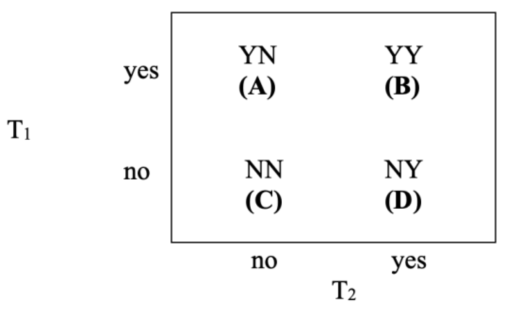
Figure 2.
Punnett cube for expanded McNemar test. The series of letters in each portion of the cube represent the outcomes of the first, second, and third trials respectively.
Figure 2.
Punnett cube for expanded McNemar test. The series of letters in each portion of the cube represent the outcomes of the first, second, and third trials respectively.
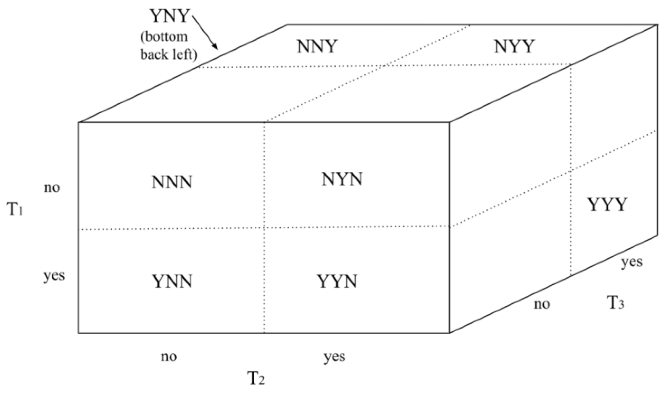
Figure 3.
Dichotomous portions of Punnett cube for Expanded McNemar test. The Punnett squares display combination of “yes” and “no” options for responses in Trial 1 and Trial 2, in Trial 2 and Trial 3, and in Trial 1 and Trial 3.
Figure 3.
Dichotomous portions of Punnett cube for Expanded McNemar test. The Punnett squares display combination of “yes” and “no” options for responses in Trial 1 and Trial 2, in Trial 2 and Trial 3, and in Trial 1 and Trial 3.
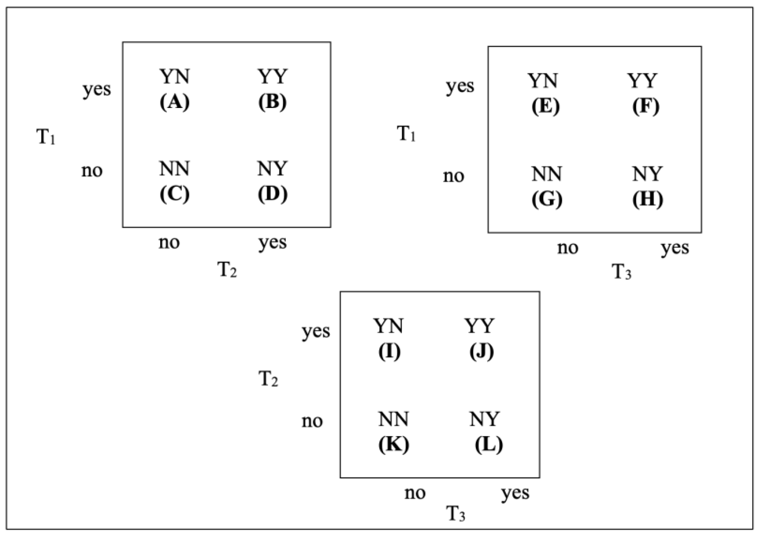
Figure 4.
Punnett cube for sample data. The series of letters in each portion of the cube represent the outcomes of the first, second, and third trials respectively. Values represent frequencies of the respective outcome combinations.
Figure 4.
Punnett cube for sample data. The series of letters in each portion of the cube represent the outcomes of the first, second, and third trials respectively. Values represent frequencies of the respective outcome combinations.
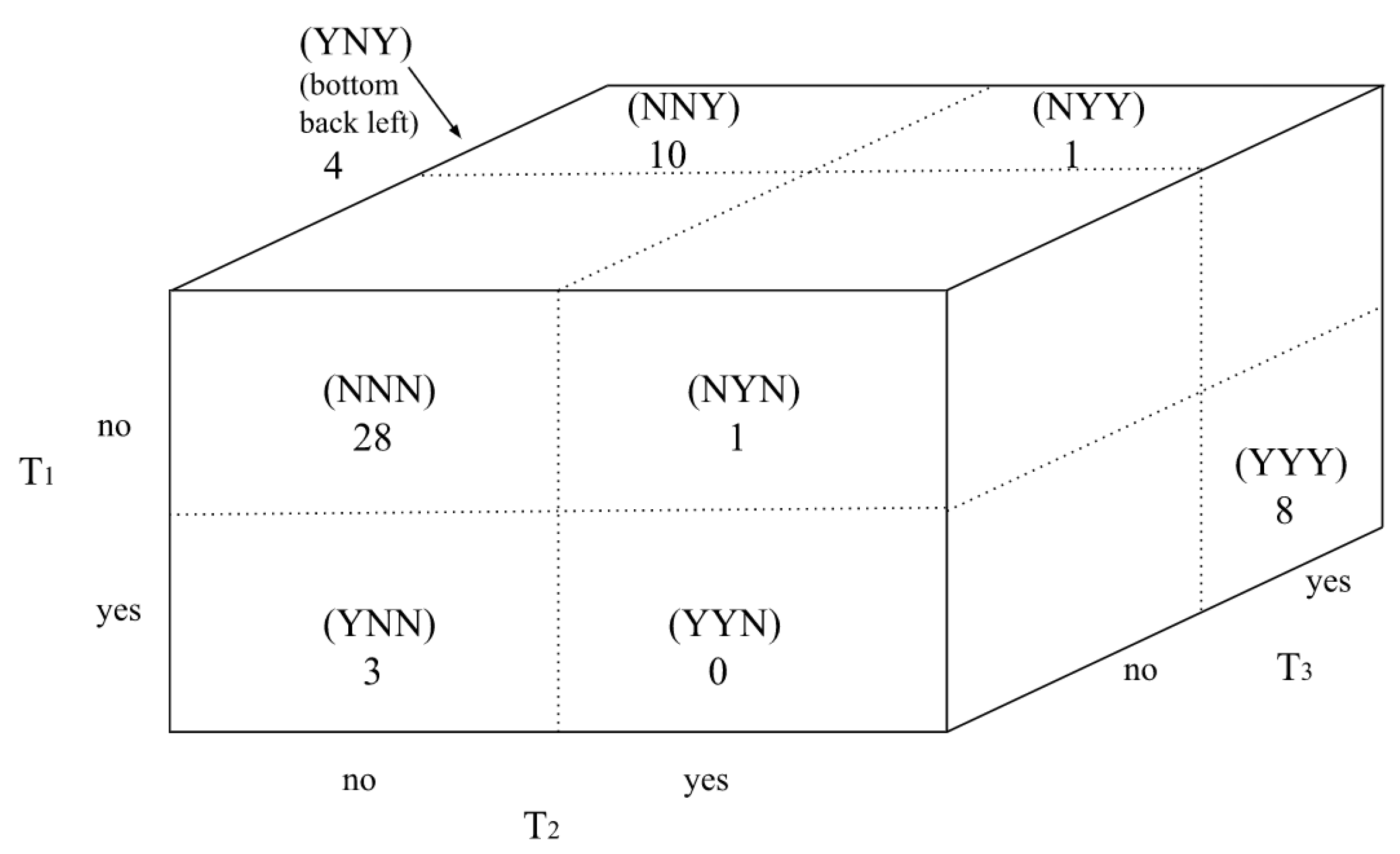
Figure 5.
Dichotomous portions of Punnett cube for sample data. Each of the Punnett squares displays the combination of “yes” and “no” options for two of the trials that serve as the basis for the Punnett cube in Figure 4. Values represent frequencies.
Figure 5.
Dichotomous portions of Punnett cube for sample data. Each of the Punnett squares displays the combination of “yes” and “no” options for two of the trials that serve as the basis for the Punnett cube in Figure 4. Values represent frequencies.
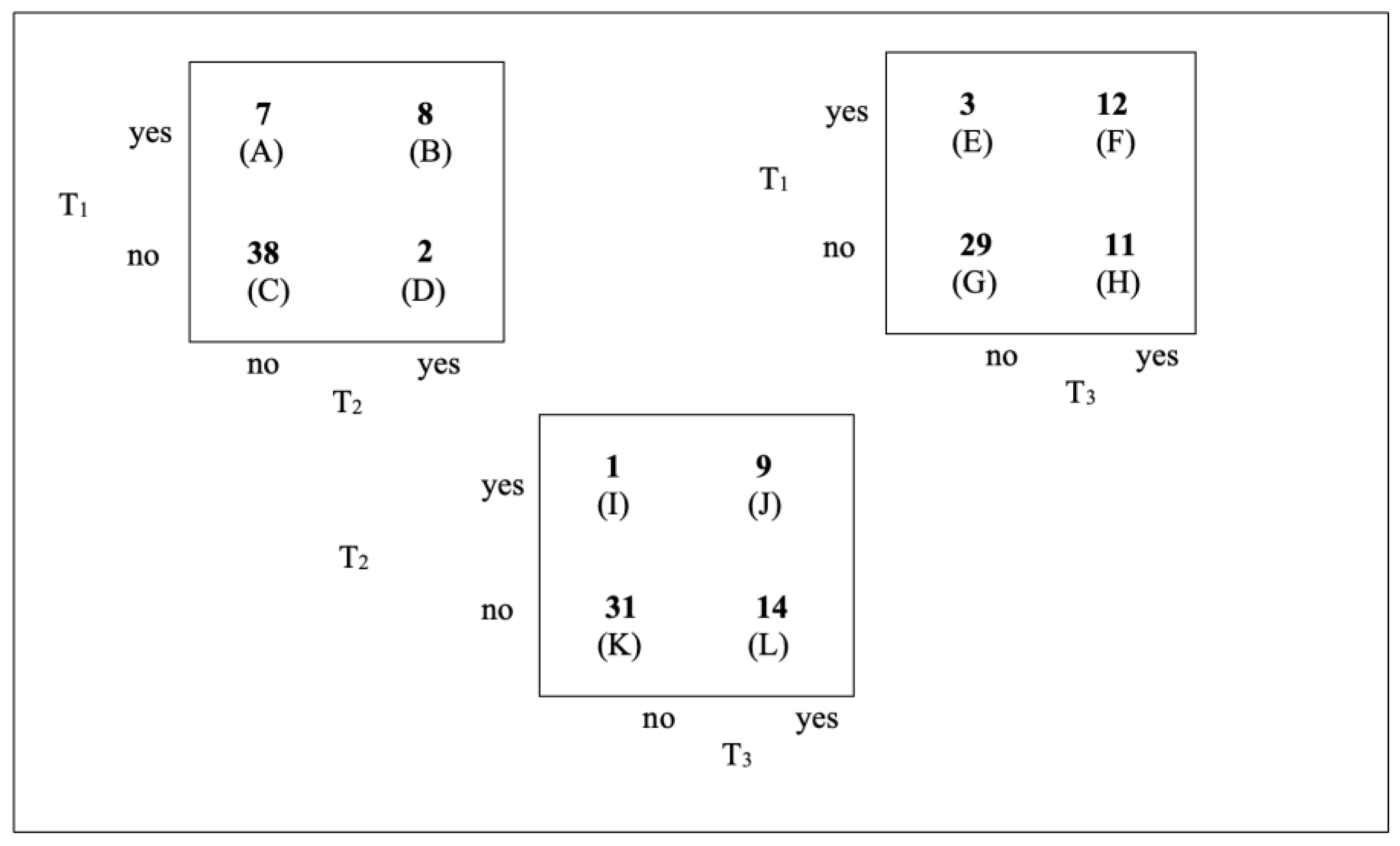
Figure 6.
Relationship between Standard, McNemar’s, and Repeated Measures chi-square tests. The repeated measures test evaluates differences in frequencies with infinite independent variable conditions and without mutually-exclusive variables.
Figure 6.
Relationship between Standard, McNemar’s, and Repeated Measures chi-square tests. The repeated measures test evaluates differences in frequencies with infinite independent variable conditions and without mutually-exclusive variables.

Table 1.
Data with Repeated Measures.
| TIME RELATIVE TO VIEWING | ||||||
|
before (1) |
during (2) |
after (3) |
||||
| HIGH BLOOD PRESSURE? |
no (1) |
f11 | f12 | f13 | f1• | |
|
yes (2) |
f21 | f22 | f23 | f2• | ||
| f•1 | f•2 | f•3 | ||||
Each cell contains the frequency for a particular combination of blood pressure category and time relative to viewing a horror movie. Marginal values f•1, f•2, and f•3, represent the total frequencies for columns. Assuming a dropout rate of 0, f•1=f•2=f•3 because the three trials involve the same subject group. Marginal values of f1• and f2• represent frequencies for rows.
Table 2.
Change Summary Table.
| Trial Outcomes | Cells |
| yes to no | A+E+I |
| no change | B+C+E+G+J+K |
| no to yes | D+H+L |
The column on the right identifies cells from Figure 3 that correspond to the presence and manner of change from an intial to a subsequent trial. Values in cells corresponding to changed responses, A, E, I, D, H, and L, become relevant to the analysis.
Disclaimer/Publisher’s Note: The statements, opinions and data contained in all publications are solely those of the individual author(s) and contributor(s) and not of MDPI and/or the editor(s). MDPI and/or the editor(s) disclaim responsibility for any injury to people or property resulting from any ideas, methods, instructions or products referred to in the content. |
© 2025 by the authors. Licensee MDPI, Basel, Switzerland. This article is an open access article distributed under the terms and conditions of the Creative Commons Attribution (CC BY) license (http://creativecommons.org/licenses/by/4.0/).
Copyright: This open access article is published under a Creative Commons CC BY 4.0 license, which permit the free download, distribution, and reuse, provided that the author and preprint are cited in any reuse.


