Submitted:
26 March 2025
Posted:
27 March 2025
You are already at the latest version
Abstract
Ambient fine particulate matter of size less than 2.5 µm in aerodynamic diameter (PM2.5) is a key component of ambient air pollution that has been linked to numerous adverse health outcomes. Reliable estimates of PM2.5 are important for supporting epidemiologic and health impact assessment studies. Precise measurements of PM2.5 are available through networks of monitors, however these are spatially sparse and temporally incomplete. Chemical transport model (CTM) simulations and satellite-retrieved aerosol optical depth (AOD) measurements are two data sources that have been used to develop prediction models for PM2.5 at fine spatial resolutions with increased spatial coverage. As part of the Multi-Angle Imager for Aerosols (MAIA) project, a geostatistical regression model has been developed to bias-correct AOD, followed by Bayesian ensemble averaging to gap-fill missing AOD values with CTM simulations. Here we present a suite of statistical software (available in the R package ensembleDownscaleR) to facilitate the adaptation of this modeling approach to other settings and air quality modeling applications. We describe the Bayesian ensemble averaging approach, model specifications, estimation methods and evaluation via cross-validation that are implemented in the software. We also provide a case study of estimating PM2.5 using 2018 data from the Los Angeles metropolitan area with an accompanying tutorial. All code is fully reproducible and available at GitHub, data is made available at Zenodo, and the ensembleDownscaleR package is available for download at GitHub.
Keywords:
Bayesian ensemble
; geostatistical downscaler
; gap-filling
; R package
; AOD
; CTM
; PM2.5
; air pollution
; spatial
1. Introduction
Exposure to ambient air pollution is a well established risk factors for multiple adverse health outcomes. Particulate matter of size less than 2.5 m in diameter () has been shown to be especially harmful due to its ability to penetrate deep into the respiratory system [1,2,3,4,5,6]. represents a chemically diverse mixture of pollutants and its major sources include electricity generation, motor vehicles, and wildland fires. Accurate estimation of concentration is an important component of air pollution health research [7,8].
Network of monitors established for regulatory purposes provide precise, direct measurements of . However these monitors are relatively expensive to install and maintain, and therefore are both spatially sparse and preferentially located in prioritized areas. There exist two additional data sources that are highly correlated with , which enable the development of methods to predict beyond locations with ground monitors. The first is outputs from chemical transport model (CTM) which provide simulations of air quality based on emission, physical processes and meteorological data. Gridded CTM simulations provide complete spatial coverage, but require bias-correction with observations due to uncertainties in model input, discretization, and other sources of errors [9].The second is satellite measurements of aerosol optical depth (AOD), which provide measures of aerosol for the entire atmospheric column at finer spatial resolution than CTM [10,11,12]. But AOD also requires bias-correction and is subject to high missingness due to cloud cover and retrieval error [13,14,15].
An important and active area of air pollution exposure assessment research is the development of methods that can utilize both AOD and CTM to predict to address limitations associated with each data type. One such framework combines predictions from geostatistical models trained separately from AOD or CTM using Bayesian ensemble averaging [16]. This approach utilizes all available monitoring, AOD, and CTM data, and provides fine-scale estimates when AOD is available, and gap-filled estimates from CTM when AOD is missing. Probabilistic uncertainty quantification for each prediction is also available through prediction interval and standard deviation. This framework has been adopted by the Multi-Angle Imager for Aerosols (MAIA) project to estimate daily , , and speciated major components in multiple large population centers around the world [17].
Here we introduce an R package, ensembleDownscaleR, containing a suite of functions to facilitate the adaptation of this modeling approach to other settings and air quality modeling applications. We describe the statistical method from [16], as well as model extensions implemented for MAIA. We also detail the functionality of the R package and provide an example analysis using 2018 data from the Los Angeles metropolitan area to estimate daily at 1km spatial resolution. This work is structured as a tutorial designed to guide practitioners in the use of the ensembleDownscaleR R package. Each stage includes a methodological introduction, code examples applied to Los Angeles dataset, and corresponding results. We make the data available at Zenodo and provide all code used for model fitting, data processing, and plot/table creation at GitHub, to ensure full reproducibility of results and assist users in their own analyses. The ensembleDownscaleR R package is available for download at GitHub.
2. Case Study Data
Our analyses correspond to a spatial region overlapping the Los Angeles metropolitan area ranging from -120.50 to -115.75 longitude, and from 32.00 to 35.70 latitude, and a temporal range of January 1st, 2018, to December 31st, 2018 (Figure 1). This region contained 60 monitoring stations from the Air Quality System (AQS) that provide hourly measurements, which we aggregate to daily averages.
AOD data were obtained from the Multi-Angle Implementation of Atmospheric Correction (MAIAC) with a spatial resolution of 1 km. Chemical transport model (CTM) data were obtained from the Community Multiscale Air Quality (CMAQ) model, which provides daily PM2.5 simulations at a 12 km spatial resolution [18]. We spatially linked the AQS monitor, AOD and CTM data using the MAIAC 1 km grid for modeling fitting and prediction.
Additional spatial land use and spatio-temporal meteorological covariates are matched to both monitor locations and grid cells. These include elevation (elevation), population density (population), cloud cover (cloud), east-west wind velocity (u_wind), north-south wind velocity (v_wind), height of planetary boundary layer (hpbl), shortwave radiation (short_rf), and humidity at two meters above the ground (humidity_2m). Additional details on the source of each covariate and spatial resolutions are detailed in the supporting information.
3. Methods and Results
In this section we provide a case study for all stages of the Bayesian ensemble fitting and prediction process on the case study. For each stage we detail the methods used, provide code examples to illustrate the use of relevant ensembleDownscaleR package functions, and present corresponding results. We break up this complete workflow for producing Bayesian ensemble predictions into six stages, detailed as follows.
- Fit two separate Bayesian downscaler regression models, and , on the monitoring PM2.5 data, one spatially and temporally matched with CTM data and the other matched with AOD data, following the form , where X is either AOD or CTM, and and are additional spatial and spatio-temporal covariates respectively.
- Produce estimates of PM2.5 (posterior predictive means) and variances for all locations using from stage 1. Produce estimates of means and variances for all times and locations for which AOD is available, using .
- Use cross-validation to produce two sets of out-of-sample PM2.5 prediction means and variances using the same data and model form as in stage 1. This produces two datasets of out-of-sample prediction means and variances for each monitor observation.
- Estimate spatially varying weights from the out-of-sample prediction mean and variances from stage 2 and the monitor PM2.5 measurements.
- Use Gaussian Process spatial interpolation (krigging) to predict weights for all grid cells in the study area.
- Use the fitted models from stage 1 and the weight estimates from stage 4 to acquire ensemble predictions of at each grid cell in the study area.
The Los Angeles dataset included 60 monitoring stations, 15,821 observation-CTM pairs, 11,668 observation-AOD pairs and 122,735 prediction grid cells. The total computation time with 25,000 Markov chain Monte Carlo (MCMC) iterations per model fit (for two stage 1 model fits, 20 stage 3 model fits, and one stage 4 model fit), took approximately 11.29 hours on an Apple MacBook Pro laptop with an Apple M3 Max processor and 36 GB of RAM.
3.1. Stage 1: Downscaler Regression Model
This section details the model specifications available for Bayesian downscaler regression model fitting using the grm() function.
3.1.1. Model
The Bayesian downscaler regression model is formulated as a spatial-temporal regression of PM2.5 against X, which is either AOD or CTM depending on user input.
The statistical model is as follows:
where and are the spatial-temporal intercept and AOD/CTM slope of the regression model at location s and time t, and are fixed effects for spatial and spatio-temporal covariates and respectively, and . Here is modeled with an inverse Gamma prior distribution, , where and hyperparameters are specified with the sigma.a and sigma.b arguments in the grm() function. For these and the remainder of the hyperparameter arguments, defaults are set to represent uninformative priors.
The slope and intercept parameters are composed of the following additive spatial and temporal random effects and fixed effects:
where spatial random effects follow a Gaussian Process () depending on a user-specified kernel with range parameter and distance matrix D. Temporal random effects that are set as first-order random walk. Normal priors are applied to fixed effects and with equivalence to a ridge regression shrinkage prior.
Users can specify inclusion of any combination of additive or multiplicative spatial or temporal random effects, and can input and matrices for fixed effects. For example, if the user-specifies inclusion of an additive spatial effect, a multiplicative temporal effect, and no and matrices, the intercept/slope equations would simplify as follows:
The inclusion of additive or multiplicative temporal and spatial effects is specified by the user with the include.additive.temporal.effect,
include.multiplicative.temporal.effect, include.additive.spatial.effect, and include.multiplicative.spatial.effect arguments in the grm() function.
3.1.2. Spatial Random Effects
The spatial random effects are modeled using Gaussian Processes (GP), with the covariance kernel specified by the user. We provide four covariance kernels for the spatial random effects: exponential, and Matérn for , where:
We also allow for the user to specify a custom covariance kernel, which must be positive definite and symmetric and parametrized with respect to the range parameter and distance d such that .
While non-additive spatio-temporal effects are not currently implemented, we provide the option to use different sets of spatial effects for different time periods. By using different spatial effects for say seasons or months, some temporal variation in spatial effects can be accounted for. Regardless of number of spatial effect sets, Gaussian process parameters (, ) are shared across sets. For example, if spatial-time sets are specified for seasons, the additive spatial random effect is as follows:
where n is the number of spatial locations and ⊗ is the Kronecker product.
Priors are placed on the Gaussian process parameters and such that and , where , , , and are specified by the user using the tau.alpha.a, tau.alpha.b, theta.alpha.a, and theta.alpha.b arguments in the grm() function. While most parameters in the Bayesian downscaler regression model are sampled with Gibbs updates, the parameter is sampled with a Metropolis-Hastings step. We employ a log-normal proposal distribution with a user-specified tuning parameter , such that . The user can specify the tuning parameter using the theta.alpha.tune argument in the grm() function, as well as the initial value for using the theta.alpha.init argument. Prior specifications and hyperparameter arguments are similar for and .
3.1.3. Temporal Random Effects
The first-order random walk temporal random effects () are specified such that,
with similarly specified. To reduce computation burden, each is discretized as evenly spaced values between 0 and 1, and each determines the temporal smoothness level. Initial values for and can be specified by the user using the rho.alpha.init and rho.beta.init arguments in the grm() function. An inverse gamma prior is place on and such that and . The user can specify the hyperparameters , , , and using the omega.alpha.a, omega.alpha.b, omega.beta.a, and omega.beta.b arguments in the grm() function.
3.1.4. Fixed Effects
The user is able to specify inclusion of fixed effects and for spatial and spatio-temporal covariates, and , respectively. The fixed effects are modeled with normal priors, and where inverse gamma priors are placed on the and parameters such that and . Thus the parameters share the same hyperparameter settings as those for , specified by the user using the and arguments in the grm() function.
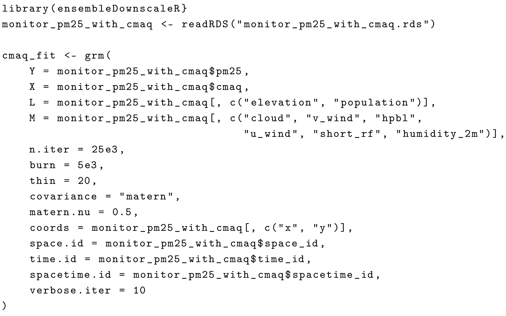
3.1.5. Stage 1 Code Example
We load the ensembleDownscaleR package and fit the Bayesian downscaler regression models for CTM using the previously described Los Angeles dataset. The code for fitting the AOD model is omitted for brevity, but is similar to the CTM model fit and is included in the tutorial code at GitHub.
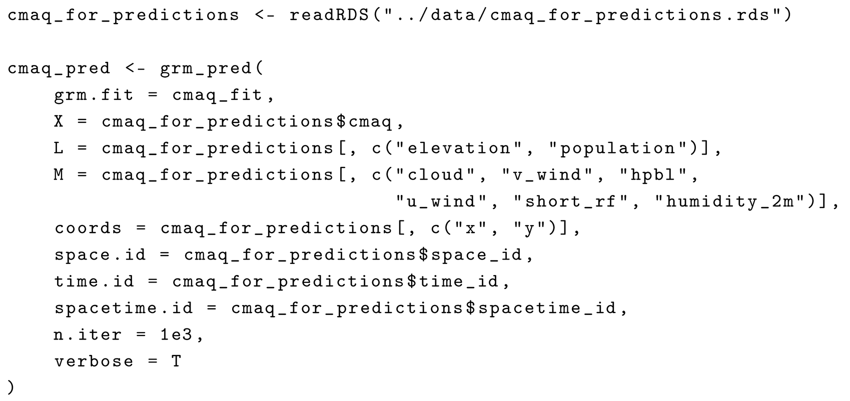
3.2. Stage 2: Produce PM2.5 Estimates and Predictions with Available CTM and AOD Data
CTM data is available for all times and locations in the study area while AOD data availability depends on time period. In this stage we use the grm_pred() to produce posterior predictive means and variances for all CTM and AOD data variables. For example, we first input the fitted model and CTM data for all times and locations in the study area, to produce and for all locations s and times t. We then input the fitted model and the sparser AOD data, to produce and for all times and locations for which AOD data is available. We note that grm_pred() outputs NA values for prediction data with locations identical to monitor locations because in this case the observed concentrations can be used.
3.2.1. Stage 2 code example
Using the fitted downscaler regression models from stage 1, we now produce full PM2.5 predictions for all locations and times in the study area using the CTM-based fitted model, and for all locations and times for which AOD is available using the AOD-based fitted model (Figure 2). The code for producing AOD predictions is omitted here, but is included in the full tutorial code at GitHub.
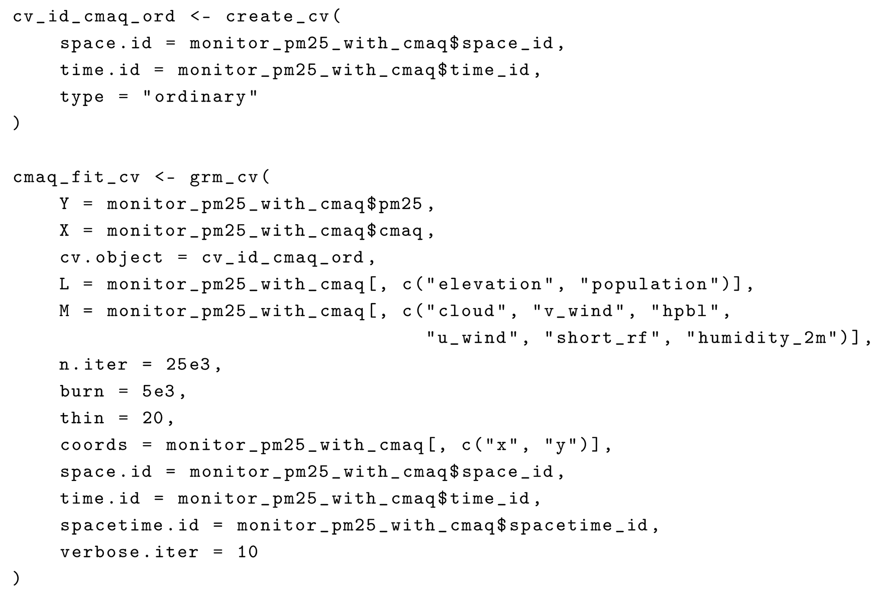
3.3. Stage 3: Use Cross-Validation to Produce out-of-Sample Prediction Means and Variances
3.3.1. Cross-Validation Details
K-fold cross-validation prevents overfitting by separating the data set into k number of folds, iteratively fitting the model to folds and predicting the remaining fold. We provide two functions to perform k-fold cross-validation with the geostatistical regression model. The first is the function create_cv() which creates cross-validation indices according to a user specified sampling scheme. The second function, grm_cv(), returns the out-of-sample PM2.5 predictions, calculated according to user inputted cross-validation indices (either obtained from the create_cv() function or created by the user), and arguments similar to those used for the grm() function to specify the downscaler regression model. The out-of-sample predictions are stacked into a dataset of the same length and order as the original dataset on which the cross-validation is applied.
The create_cv() allows specification of the following types of cross-validation (Figure 3):
- Ordinary: Folds are randomly assigned across all observations
- Spatial: Folds are randomly assigned across all spatial locations.
- Spatial Clustered: K spatial clusters are estimated using k-means clustering on spatial locations. These clusters determine the folds.
- Spatial Buffered: Folds are randomly assigned across all spatial locations. For each fold, observations are dropped from the training set if they are within a user-specified distance from the nearest test set point.
In Figure 3 we visually detail how the folds are assigned for each type of cross-validation, using the monitor locations and times in our study area as an example and assuming 5 cross-validation folds. We plot all fold assignments for four randomly chosen days, for ordinary, spatial, spatial clustered cross-validation, with color representing fold assignment. For the spatial buffered cross-validation we plot only one fold assignment, with color representing if a location is in the first test fold, the first training fold, or dropped due to being within a 30km buffer of a location in the first test fold.
When assigning folds we enforce that each fold contains at least one observation from each spatial location and spacetime indicator. Locations for which there are fewer observations than folds should be filtered out of the dataset prior to analysis. Data from the first and last time point are left unassigned, and out-of-sample predictions for these data are output as missing data. If the out-of-sample dataset has a larger temporal range than the in-sample dataset for a given fold, the out-of-sample predictions for the extra time points are also output as missing data.
3.3.2. Producing out-of-Sample Prediction Means and Variance
The grm_cv() function uses the previously detailed cross validation indices and model specifications to produce estimates of and , where is the is value at location s, time t, and and are the posterior predictive distributions based on models and respectively, the downscaler regression models. Specifically, grm_cv() outputs posterior predictive means and variances that are used in stage 4 to fit the full ensemble model.
3.3.3. Stage 3 Code Example
We now create the cross-validations indices with the create_cv() function for both AOD and CTM linked monitors, and then use the grm_cv() function to produce out-of-sample PM2.5 predictions for all monitor observations, for both the CTM and AOD data. The code for producing AOD out-of-sample predictions is omitted here, but is included in the tutorial code at GitHub.
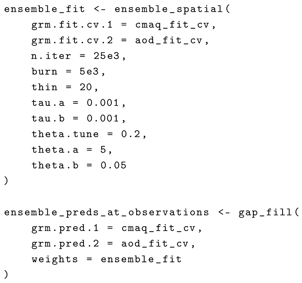
3.4. Stage 4: Estimate Spatially Varying Weights
At this stage we use the ensemble_spatial() function to fit the ensemble model , where are spatially varying weights. We estimate the weights by fitting the ensemble model on the out-of-sample predictions produced during stage 3,
and , and the original data at all times and a monitor locations. We place a Gaussian Process prior on the weights, , where is an exponential kernel, and and are the distance and range parameters, respectively. Similar to the spatial processes in stage 1, we place an inverse gamma prior on and a gamma prior on , such that and . The user can specify the hyperparameters , , , and using the tau.a, tau.b, theta.a, and theta.b arguments in the ensemble_spatial() function.
The ensemble_spatial() function accepts the output from grm_cv() in stage 3 as input, and outputs the full posterior distribution samples of where .
3.4.1. Stage 4 Code Example
At this stage we estimate the spatially varying weights for the ensemble model, using the out-of-sample predictions produced in stage 3, and the original monitor PM2.5 measurements.
We display the out-of-sample predictions produced in stage 3 to these ensemble weight estimates and the original monitor measurements, while including the weight estimates for reference (Figure 4). If desired, one can additionally use these weight estimates with the gap_fill() function to produce ensemble-based predictions for each location at which is observed, though these outputs are not used in later stages. We do this here to compare the ensemble model performance to the CTM-based and AOD-based models on the times and locations for which both CTM and AOD data are observed, employing ordinary, spatial, spatial-clustered, and spatial-buffered cross-validation for each model (Table 1, see supplementary materials for more details). For all cross-validation formulations, the ensemble model outperforms both the CTM-based and AOD-based models in terms of RMSE and , while maintaining accurate 95% prediction interval coverage. Note that gap_fill() function uses the weight estimates to produce ensemble-based predictions for times and locations at which both CTM and AOD data are observed, and fills in the remaining times and locations with the CTM-based predictions.
3.5. Stage 5: Predict Weights for All Locations
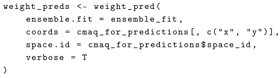
At this stage we use the weight_pred() function to spatially interpolate the posterior samples of garnered in stage 4, across all 1km x 1km grid cells in the study area. Specifically where , with output from stage 4. These weights are used in the final stage to produce ensemble-based predictions for all locations in the study area.
3.5.1. Stage 5 Code Example
We spatially interpolate the posterior samples of from stage 4 across all locations in the study area using the weight_pred() function. (Figure 5). This provides the weights used in the final stage to produce full ensemble estimates for all times and locations in the study area.
3.6. Stage 6: Compute Ensemble Predictions for All Locations
The last stage comprises using the posterior means and variances for all CTM and AOD data produced in stage 2, and the spatially interpolated weights from stage 5, to compute posterior predictive means and variances for all times t and locations s in the study area, done with the gap_fill() function.
For times and locations for which both CTM and AOD are observed, gap_fill() outputs ensemble-based estimates, where and . For times and locations for which solely CTM is available, gap_fill() outputs posterior predictive means and variances identical to those produced in stage 2 from .
3.6.1. Stage 6 Code Example
Here we input the posterior means and variances for all CTM and AOD data produced in stage 2, and the spatially interpolated weights from stage 5, into the gap_fill() function, which outputs posterior predictive means and variances for all times t and locations s in the study area (Figure 5).
4. Discussion
In this work we introduce the ensembleDownscaleR package for fitting Bayesian geostatistical regression and ensemble models, designed for predicting PM2.5 using CTM simulations and AOD measurements. We also provide a code tutorial based on a case study of Los Angeles metropolitan area data from 2018. The purpose of this work is guide practitioners in generating robust PM2.5 predictions and uncertainty quantification with a flexible and well-documented software workflow. The framework can also be applied to other air pollutants and data integration problems.
There are areas for future improvement that are worth noting. The Gaussian Process spatial random effects employed by our model are appropriate for the size of the Los Angeles case study data used here. For much larger datasets (with many more monitors and/or much larger prediction grids) the inference of the Gaussian Process parameters will be prohibitively slow. Incorporation of scalable random processes, such as Nearest Neighbor Gaussian Processes [19], could make these methods feasible for much larger datasets than those assessed here. Furthermore, spatial covariance specifications are currently limited to isotropic, stationary kernels. There are cases where PM2.5 data may exhibit correlation that suggests anisotropic or nonstationary kernels would be more appropriate, such as data that includes periods with high wind or localized wildfires. Inclusion of covariates such as wind information can often resolve this. Inspecting residual correlation and covariance parameter can ensure that the covariance is reasonably specified for a given dataset. Finally, the current software does not support integrated parallelization. For example, the grm_cv function fits a model on each cross-validation fold sequentially rather than exploiting multiple cores or compute nodes to fit each model concurrently. Model fitting time could be substantially lowered without sacrificing software ease-of-use by incorporating parallelization specifications directly in the ensembleDownscaleR package functions.
Supplementary Materials
Codes for replicating the analyses in this paper are provided at GitHub. Additional figures, tables, and details are available at: Preprints.org, Table S1: Data dictionary for monitor_pm25_with_cmaq dataset; Table S2: Data dictionary for monitor_pm25_with_aod dataset; Table S3: Data dictionary for cmaq_for_predictions dataset; Table S4: Data dictionary for aod_for_predictions dataset; Table S5: Posterior mean spatial random effects.
Author Contributions
Conceptualization, W.M. and H.C.; methodology, W.M. and H.C.; software, W.M. and H.C.; validation, W.M. and M.Q.; formal analysis, W.M. and H.C.; investigation, W.M. and H.C.; resources, H.C. and Y.L.; data curation, W.M., Y.L., and Y.L.; writing—original draft preparation, W.M.; writing—review and editing, M.Q., Y.L., and H.C; visualization, W.M. and M.Q.; supervision, H.C.; project administration, Y.L. and H.C.; funding acquisition, Y.L and H.C. All authors have read and agreed to the published version of the manuscript.
Funding
This work was partially supported by the NASA MAIA investigation led by D. Diner (Subcontract #1558091). It has not been formally reviewed by NASA. The views expressed in this document are solely those of the authors and do not necessarily reflect those of the NASA. NASA does not endorse any products or commercial services mentioned in this publication.
Informed Consent Statement
Not applicable
Data Availability Statement
Conflicts of Interest
The authors declare no conflicts of interest.
References
- Apte, J.S.; Marshall, J.D.; Cohen, A.J.; Brauer, M. Addressing global mortality from ambient PM2. 5. Environmental science & technology 2015, 49, 8057–8066. [Google Scholar]
- Fu, P.; Guo, X.; Cheung, F.M.H.; Yung, K.K.L. The association between PM2. 5 exposure and neurological disorders: a systematic review and meta-analysis. Science of the Total Environment 2019, 655, 1240–1248. [Google Scholar] [CrossRef] [PubMed]
- Yuan, S.; Wang, J.; Jiang, Q.; He, Z.; Huang, Y.; Li, Z.; Cai, L.; Cao, S. Long-term exposure to PM2. 5 and stroke: a systematic review and meta-analysis of cohort studies. Environmental research 2019, 177, 108587. [Google Scholar] [CrossRef] [PubMed]
- Alexeeff, S.E.; Liao, N.S.; Liu, X.; Van Den Eeden, S.K.; Sidney, S. Long-term PM2. 5 exposure and risks of ischemic heart disease and stroke events: review and meta-analysis. Journal of the American Heart Association 2021, 10, e016890. [Google Scholar] [CrossRef] [PubMed]
- Fan, J.; Li, S.; Fan, C.; Bai, Z.; Yang, K. The impact of PM2. 5 on asthma emergency department visits: a systematic review and meta-analysis. Environmental Science and Pollution Research 2016, 23, 843–850. [Google Scholar] [CrossRef] [PubMed]
- Gong, C.; Wang, J.; Bai, Z.; Rich, D.Q.; Zhang, Y. Maternal exposure to ambient PM2. 5 and term birth weight: a systematic review and meta-analysis of effect estimates. Science of The Total Environment 2022, 807, 150744. [Google Scholar] [CrossRef] [PubMed]
- Shaddick, G.; Thomas, M.L.; Amini, H.; Broday, D.; Cohen, A.; Frostad, J.; Green, A.; Gumy, S.; Liu, Y.; Martin, R.V.; et al. Data integration for the assessment of population exposure to ambient air pollution for global burden of disease assessment. Environmental science & technology 2018, 52, 9069–9078. [Google Scholar]
- Van Donkelaar, A.; Hammer, M.S.; Bindle, L.; Brauer, M.; Brook, J.R.; Garay, M.J.; Hsu, N.C.; Kalashnikova, O.V.; Kahn, R.A.; Lee, C.; et al. Monthly global estimates of fine particulate matter and their uncertainty. Environmental Science & Technology 2021, 55, 15287–15300. [Google Scholar]
- Appel, K.W.; Bash, J.O.; Fahey, K.M.; Foley, K.M.; Gilliam, R.C.; Hogrefe, C.; Hutzell, W.T.; Kang, D.; Mathur, R.; Murphy, B.N.; et al. The Community Multiscale Air Quality (CMAQ) model versions 5.3 and 5.3. 1: system updates and evaluation. Geoscientific Model Development Discussions 2020, 2020, 1–41. [Google Scholar] [CrossRef] [PubMed]
- Xiao, Q.; Chang, H.H.; Geng, G.; Liu, Y. An ensemble machine-learning model to predict historical PM2. 5 concentrations in China from satellite data. Environmental science & technology 2018, 52, 13260–13269. [Google Scholar]
- Zhang, D.; Du, L.; Wang, W.; Zhu, Q.; Bi, J.; Scovronick, N.; Naidoo, M.; Garland, R.M.; Liu, Y. A machine learning model to estimate ambient PM2. 5 concentrations in industrialized highveld region of South Africa. Remote sensing of environment 2021, 266, 112713. [Google Scholar] [CrossRef] [PubMed]
- Chu, Y.; Liu, Y.; Li, X.; Liu, Z.; Lu, H.; Lu, Y.; Mao, Z.; Chen, X.; Li, N.; Ren, M.; et al. A review on predicting ground PM2. 5 concentration using satellite aerosol optical depth. Atmosphere 2016, 7, 129. [Google Scholar] [CrossRef]
- Kianian, B.; Liu, Y.; Chang, H.H. Imputing satellite-derived aerosol optical depth using a multi-resolution spatial model and random forest for PM2. 5 prediction. Remote Sensing 2021, 13, 126. [Google Scholar] [CrossRef]
- Xiao, Q.; Geng, G.; Cheng, J.; Liang, F.; Li, R.; Meng, X.; Xue, T.; Huang, X.; Kan, H.; Zhang, Q.; et al. Evaluation of gap-filling approaches in satellite-based daily PM2. 5 prediction models. Atmospheric Environment 2021, 244, 117921. [Google Scholar] [CrossRef]
- Pu, Q.; Yoo, E.H. A gap-filling hybrid approach for hourly PM2. 5 prediction at high spatial resolution from multi-sourced AOD data. Environmental Pollution 2022, 315, 120419. [Google Scholar] [CrossRef] [PubMed]
- Murray, N.L.; Holmes, H.A.; Liu, Y.; Chang, H.H. A Bayesian ensemble approach to combine PM2.5 estimates from statistical models using satellite imagery and numerical model simulation. Environmental Research 2019, 178, 108601. [Google Scholar] [CrossRef] [PubMed]
- Diner, D.J.; Boland, S.W.; Brauer, M.; Bruegge, C.; Burke, K.A.; Chipman, R.; Di Girolamo, L.; Garay, M.J.; Hasheminassab, S.; Hyer, E.; et al. Advances in multiangle satellite remote sensing of speciated airborne particulate matter and association with adverse health effects: from MISR to MAIA. Journal of Applied Remote Sensing 2018, 12, 042603–042603. [Google Scholar] [CrossRef]
- Baker, K.; Woody, M.; Tonnesen, G.; Hutzell, W.; Pye, H.; Beaver, M.; Pouliot, G.; Pierce, T. Contribution of regional-scale fire events to ozone and PM2. 5 air quality estimated by photochemical modeling approaches. Atmospheric Environment 2016, 140, 539–554. [Google Scholar] [CrossRef]
- Datta, A.; Banerjee, S.; Finley, A.O.; Gelfand, A.E. Hierarchical Nearest-Neighbor Gaussian Process Models for Large Geostatistical Datasets. Journal of the American Statistical Association 2016, 111, 800–812. [Google Scholar] [CrossRef] [PubMed]
Figure 1.
The study area for the Los Angeles metropolitan area. The red dashed line defines the study area boundaries and the blue triangles mark the locations of the 60 PM2.5 monitoring stations.
Figure 1.
The study area for the Los Angeles metropolitan area. The red dashed line defines the study area boundaries and the blue triangles mark the locations of the 60 PM2.5 monitoring stations.
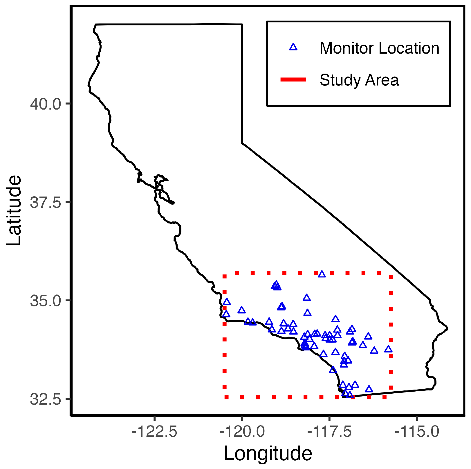
Figure 2.
For July 15th 2018 (a) PM2.5 predictions for all locations in the study area using the CTM-based fitted model. (b) Input CTM PM2.5 simulations. (c) PM2.5 predictions for all locations at which AOD is available using the AOD-based fitted model. (d) Input AOD observations.
Figure 2.
For July 15th 2018 (a) PM2.5 predictions for all locations in the study area using the CTM-based fitted model. (b) Input CTM PM2.5 simulations. (c) PM2.5 predictions for all locations at which AOD is available using the AOD-based fitted model. (d) Input AOD observations.
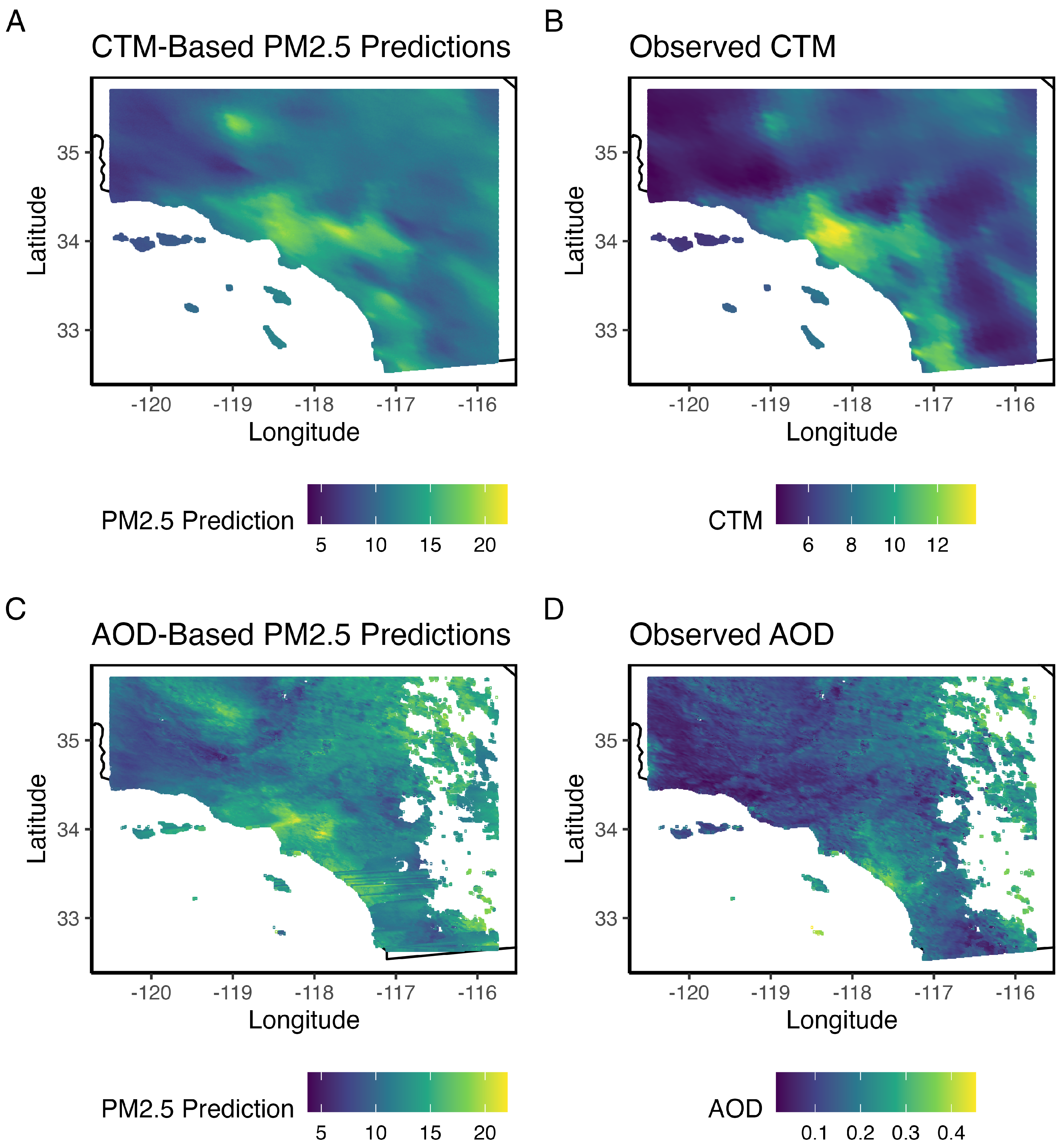
Figure 3.
Four types of cross-validation are available in the ensembleDownscaleR package: ordinary, spatial, spatial clustered, and spatial buffered. The column facets are the four randomly chosen days with near-full locations available, and the row facets are the four types of cross-validation.
Figure 3.
Four types of cross-validation are available in the ensembleDownscaleR package: ordinary, spatial, spatial clustered, and spatial buffered. The column facets are the four randomly chosen days with near-full locations available, and the row facets are the four types of cross-validation.
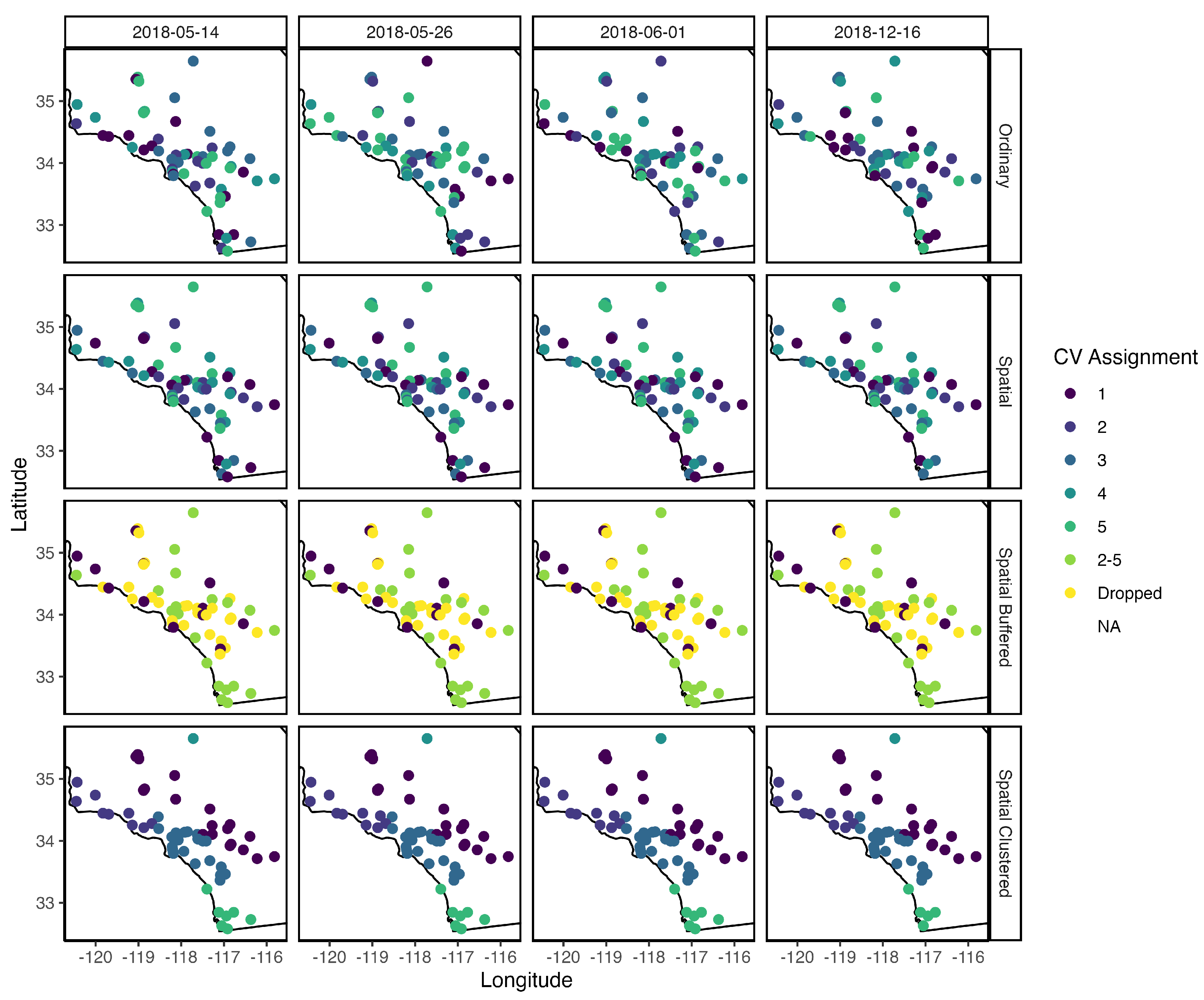
Figure 4.
(a) Monitor measurements in study area for July 15th, 2018. (b) Out-of-sample CTM-based mean estimates for July 15th, 2018. (c) Out-of-sample AOD-based mean estimates for July 15th, 2018. (d) Ensemble model spatially varying weights.
Figure 4.
(a) Monitor measurements in study area for July 15th, 2018. (b) Out-of-sample CTM-based mean estimates for July 15th, 2018. (c) Out-of-sample AOD-based mean estimates for July 15th, 2018. (d) Ensemble model spatially varying weights.
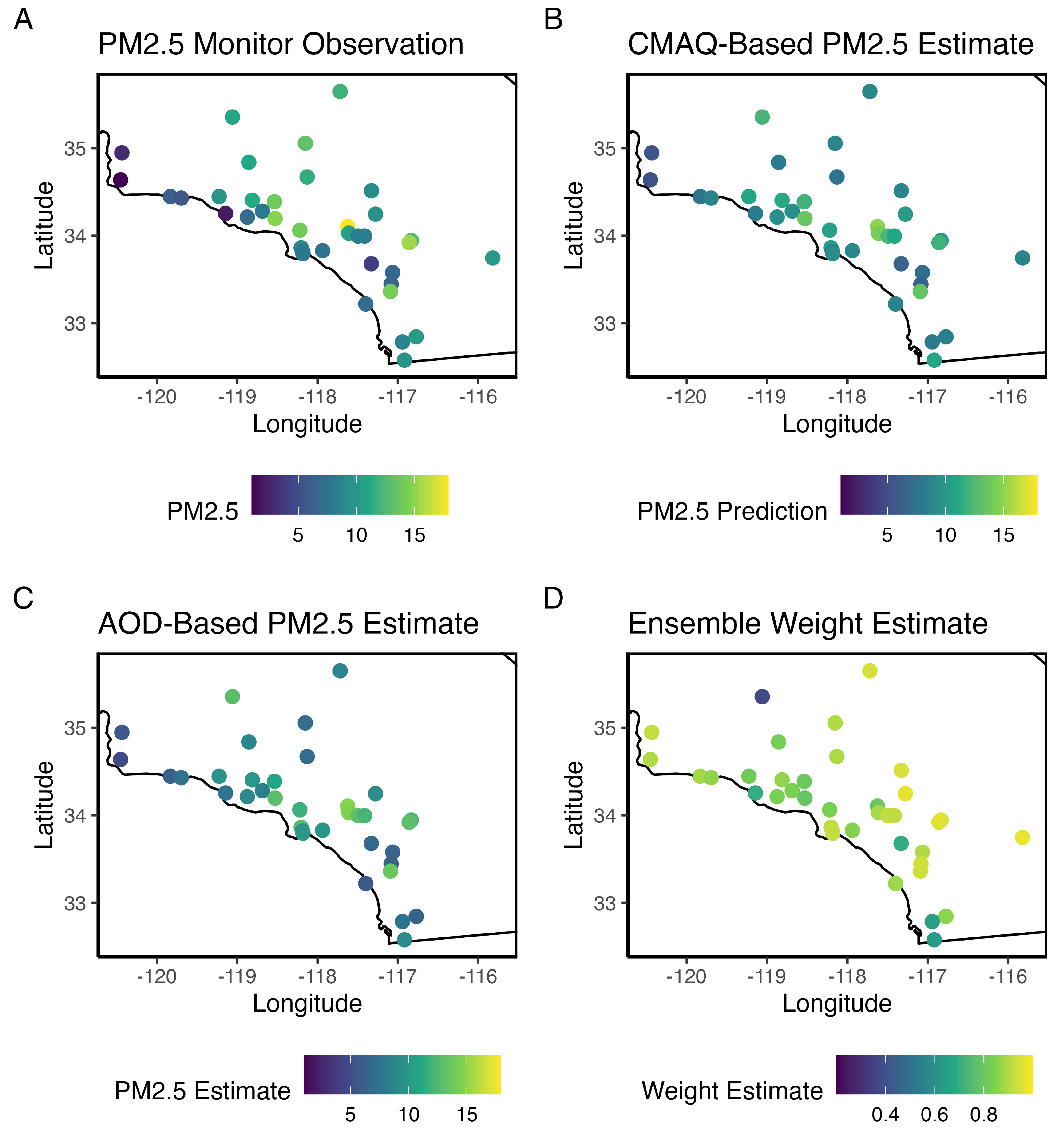
Figure 5.
(a) Posterior mean spatially interpolated weights produced in stage 5. (b) Ensemble-based posterior predictive mean estimates. (c) Ensemble-based posterior predictive standard deviation estimates.
Figure 5.
(a) Posterior mean spatially interpolated weights produced in stage 5. (b) Ensemble-based posterior predictive mean estimates. (c) Ensemble-based posterior predictive standard deviation estimates.
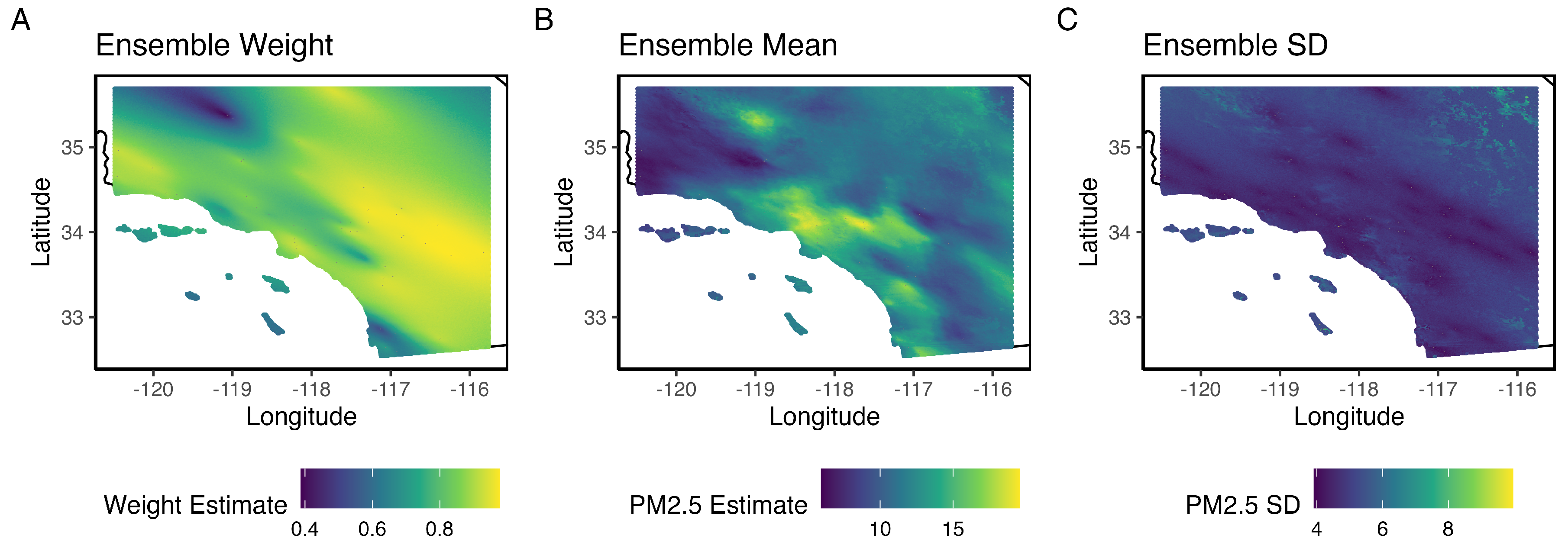

Table 1.
Model prediction performance for ensemble model from stage 4, and CTM-based and AOD-based models from stage 2, using each cross-validation type available in the create_cv() function. We assess model performance using 10-fold ordinary, spatial, spatial-clustered, and spatial-buffered cross-validation. The spatial-buffered cross-validation is formulated with buffer sizes of 12.6km and 42.6km, corresponding with approximately 0.7 and 0.3 spatial random effect correlation respectively.
| CV Type | Model | RMSE | Posterior SD | 95% PI Coverage | |
|---|---|---|---|---|---|
| Ordinary | AOD-Based | 4.401 | 0.573 | 4.273 | 0.954 |
| CMAQ-Based | 3.847 | 0.674 | 4.077 | 0.960 | |
| Ensemble | 3.713 | 0.696 | 4.223 | 0.971 | |
| Spatial | AOD-Based | 4.710 | 0.486 | 4.764 | 0.954 |
| CMAQ-Based | 4.379 | 0.555 | 4.603 | 0.957 | |
| Ensemble | 4.116 | 0.607 | 4.714 | 0.969 | |
| Spatial | AOD-Based | 4.778 | 0.471 | 4.767 | 0.953 |
| Buffered | CMAQ-Based | 6.200 | 0.109 | 5.194 | 0.950 |
| (0.3 Corr) | Ensemble | 4.349 | 0.561 | 4.988 | 0.970 |
| Spatial | AOD-Based | 4.736 | 0.480 | 4.758 | 0.952 |
| Buffered | CMAQ-Based | 4.578 | 0.514 | 4.612 | 0.955 |
| (0.7 Corr) | Ensemble | 4.243 | 0.583 | 4.758 | 0.968 |
| Spatial Clustered | AOD-Based | 5.394 | 0.325 | 5.151 | 0.945 |
| CMAQ-Based | 5.304 | 0.348 | 5.104 | 0.959 | |
| Ensemble | 4.735 | 0.480 | 5.227 | 0.966 |
Disclaimer/Publisher’s Note: The statements, opinions and data contained in all publications are solely those of the individual author(s) and contributor(s) and not of MDPI and/or the editor(s). MDPI and/or the editor(s) disclaim responsibility for any injury to people or property resulting from any ideas, methods, instructions or products referred to in the content. |
© 2025 by the authors. Licensee MDPI, Basel, Switzerland. This article is an open access article distributed under the terms and conditions of the Creative Commons Attribution (CC BY) license (http://creativecommons.org/licenses/by/4.0/).
Copyright: This open access article is published under a Creative Commons CC BY 4.0 license, which permit the free download, distribution, and reuse, provided that the author and preprint are cited in any reuse.


