

Submitted:
09 August 2026
Posted:
10 August 2026
You are already at the latest version
Abstract
We study the observational identifiability of MOND-like weak-field response dictionaries on the SPARC sample (N_gal = 91, N_points = 1782) under a full within-galaxy covariance likelihood with a learned systematic floor σ_sys. A constrained projected scalar-sector interpretation motivates the matching relation a₀ = εcH₀ and additional structural and cross-scale consistency conditions, without treating SPARC as validation of complete quaternionic gravity.For fixed H₀, that matching is one-to-one on the compared domain, so the PTQ-ν and MOND simple-ν likelihood families are analytically identical; the same reparameterization identity holds for the shared ν_q family. Within the ν_q deformation the best recovered value is q ≈ 0.984, and the present analysis does not require a material departure from the simple-ν limit under AIC. An external thickness audit (N = 19) identifies a robust kinematic–structural association after surface-density control (R² ≃ 0.818), based on a local epicyclic-frequency-like diagnostic κ_kin with dimensions of inverse time. A dimensionally valid map from κ_kin to a dimensionless PTQ geometric efficiency is not established here. Strict cross-scale equality under the selected matching relation and the adopted Ω_Λ(ε) diagnostic map fails (ε_RC ≈ 0.155 versus ε_cos ≈ 1.492). A dimensionless structural bridge that could mediate the mismatch is not established here. The paper’s contribution is therefore a constrained observational interface for PTQ-motivated weak-field phenomenology, with clear targets for future theory derivation.
Keywords:
modified gravity
; gravitational-wave speed
; MOND phenomenology
; galaxy rotation curves
; PT symmetry
; information criteria
1. Introduction
Disk-galaxy rotation curves remain one of the sharpest empirical arenas for testing MOND-like weak-field phenomenology [5,7]. The radial acceleration relation [8] and the baryonic Tully–Fisher relation [4,6] set well-established regularities that any proposed weak-field dictionary must confront. The multimessenger bound [2,3] further motivates infrared postures compatible with tensor-sector luminality [19,20,21].
We focus on the observational identifiability of weak-field response dictionaries and on the additional consistency conditions introduced by a constrained PTQ interpretation:
- Which phenomenological responses are required by SPARC under transparent parameter counting?
- Which model labels correspond to genuinely different observable radial laws?
- What structural and cross-scale diagnostics become available once a constrained projected scalar-sector interpretation is imposed?
Companion structural work on a PT-even Palatini torsion framework argues for tensor-sector coefficient locking at quadratic order [1]. Here that material is used only as structural motivation for a projected scalar-sector dictionary. It is not treated as a complete gravitational theory being validated by SPARC, and the published luminality theorem is not claimed to inherit automatically onto the exact Route-A one-form posture used below.
Contributions.
This paper provides:
- explicit observational-equivalence identification of the PTQ- and MOND simple- likelihood families under , and of the shared family (code labels ptq-screen/mond-screen);
- transparent full-covariance maximum-likelihood (MLE) accounting with corrected parameter counts including learned ;
- separation of likelihood equivalence from prior-measure effects under the priors adopted in the Bayesian analysis;
- an external kinematic–structural audit based on an independent epicyclic-frequency-like diagnostic ;
- a strict cross-scale closure stress test under an adopted diagnostic map, allowed to fail;
- an open reproducibility record in which both positive associations and failures remain visible.
Section 2 separates structural motivation, selected matching, adopted phenomenology, and the cosmological diagnostic map. Section 3 defines data, covariance, models, and parameter counts. Section 4 reports MLE comparisons, equivalence, geometry, and closure. Section 5 interprets the results; Section 6 states bounded conclusions.
2. Structural Motivation and Epistemic Layers
We organize the PTQ-facing content into four epistemic layers that must not be collapsed into one another.
2.1. Layer A: Structural Motivation
Observable scalar quantities are defined after a PT-even projection onto a real scalar sector [1,25]. The present empirical posture adopts Route A: projective equivalence is implemented by a one-form compensator treated as a non-dynamical spurion, with invariant residue
following the projective-Palatini IR residual construction [26]. A scalar representative appears only on admissible domains where is longitudinal; it is not used as a compensator for full projective invariance. Related conditional scalar-gradient / trace-torsion branch constructions [27] provide additional structural motivation for studying constrained single-response branches.
Scope.
These public structural sources motivate the constrained interpretation used below; they do not derive the SPARC likelihood dictionary, the simple- response, or the matching relation .
2.2. Layer B: Selected Weak-Field Matching Relation
The empirical dictionary anchors the acceleration scale by the matching relation
with in the analysis pipeline used in this study [22]. Equation (2) is a selected matching relation: it is dimensionally natural and enables cross-scale bookkeeping, but it is not established here as a unique first-principles prediction.
2.3. Layer C: Adopted Phenomenology
The radial response functions used in the likelihood are adopted phenomenology. We use the fixed simple- interpolating function
and the one-parameter generalization
implemented in the analysis pipeline used in this study (repository labels: ptq-screen/mond-screen). These forms are empirical realizations shared with standard MOND benchmarks; they are not derived from the upstream PTQ theorems cited for structural motivation.
2.4. Layer D: Cosmological Diagnostic Map
For the specified cross-scale stress test, we adopt the diagnostic map
with the exact inversion on ,
Equation (5) is an adopted diagnostic dictionary for that stress test, not a unique cosmological prediction established by the SPARC analysis. Alternate normalizations, when considered, enter only as sensitivity variants and are not promoted to primary equations.
3. Data, Likelihood, Models, and Parameter Accounting
3.1. Sample
We use the SPARC compilation [9]. Baseline cuts require inclination , fractional distance uncertainty , and quality flag . Table 1 records the frozen sample flow; intermediate cuts are applied jointly rather than as separately optimized stages.
For each galaxy we use radii , observed speeds , baryonic templates , and geometry used in error propagation (D, i, ).
3.2. Full Within-Galaxy Covariance
For galaxy g with residual vector of length , the primary likelihood contribution is the multivariate Gaussian
with full sample . The covariance implemented in the analysis pipeline is
where the distance and inclination Jacobians follow the linearized propagation used in the code,
with estimated by centered finite differences on the model curve. Distance and inclination therefore enter through linearized covariance propagation; they are not treated as explicitly sampled nuisance parameters that are marginalized in the likelihood. This approximation can affect absolute and descriptive model-comparison values. The analytical PTQ-/MOND identity below is unaffected when the identical covariance construction is applied consistently to both parameterizations. The global floor is learned in the fit. Radial points within a galaxy are consequently not treated as independent when evaluating Eq. (7).
3.3. Model Definitions
Let and . The implementations used here are:
Observational equivalence (identifiability).
Proposition 1
This is an observable-model identifiability result, not a new PTQ theorem. The numerical differences (simple-) and () are implementation-level verifications of the analytical identity.
Status of the deformation.
In the deep-MOND regime ,
Only recovers the usual deep-MOND scaling . The best recovered value in the present full-covariance MLE is , close to unity; the likelihood gain relative to simple- is too small to offset the additional parameter under AIC. Thus the present SPARC analysis does not require a material departure from the simple- limit within this phenomenological family. The parameter q is not treated as a derived PTQ quantity.
Independent kinematic diagnostic .
The thickness audit uses an independent single-radius kinematic diagnostic constructed from the observed rotation curve. It does not depend on fitted PTQ/MOND parameters, , , or , and it never enters the likelihood. At a representative outer-disk radius chosen by the vdisk-peak rule (radius of maximum disk contribution , falling back to maximum ), let v denote the observed circular speed and the local logarithmic slope estimated from that observed curve. Then
Dimensionally : Eq. (10) is a local epicyclic-frequency-like kinematic diagnostic, not a dimensionless geometric efficiency. A historically discussed dimensionless PTQ-inspired efficiency involving residual acceleration over and a response factor is a distinct observable; no frozen normalization identifying the two is used here. The schematic aperture concept is likewise dimensionless () and is not equated to (Appendix A).
Characteristic surface-density proxy .
When resolved per-radius surface-density profiles are unavailable, is a characteristic surface-density proxy at ,
with the frozen construction constants , (an adopted construction constant in the coded proxy), and (helium mass correction). These factors play distinct roles and are not a duplicated helium correction. The quantity is not a direct catalog surface-density measurement at every radius.
3.4. Parameter Counting
With learned and one stellar mass-to-light ratio per galaxy, the effective fitted counts used for information criteria are:

Table 2.
Effective parameter counts k including learned . Distance and inclination enter only through and are not counted. The independent kinematic diagnostic is not counted.
Table 2.
Effective parameter counts k including learned . Distance and inclination enter only through and are not counted. The independent kinematic diagnostic is not counted.
| Model family | Global (+) | k |
|---|---|---|
| Baryon | 92 | |
| MOND (simple-) | 93 | |
| PTQ linear | 93 | |
| PTQ- | 93 | |
| PTQ- / MOND- | or | 94 |
| NFW-1p | per galaxy | 183 |
Fitted bounds follow the production implementation: , for -parameterized families, , and . Global scale parameters recovered at the reported maxima lie in the interior of those intervals (e.g. for PTQ-). For the simple-/PTQ- and families, 15 per-galaxy values lie on or at the hard bounds in the reported best starts; NFW-1p shows 42 near-bound parameters in its best recovered start. Bound contact is disclosed here as optimization bookkeeping and is not reinterpreted as physical support for either family. Because some per-galaxy parameters contact hard bounds, AIC/BIC are used as descriptive complexity diagnostics rather than as a unique theory-selection authority.
4. Results
4.1. Full-Covariance MLE Accounting
Table 3 reports maximum log-likelihood values under the full-covariance objective with no priors in the optimization (block-coordinate ascent on ). AIC uses k from Table 2 [15]. uses as a descriptive accounting choice [16] and is reported only with that caveat; it is not treated as a unique theory-selection rule.
No single-IC winner narrative.
Among the listed families, NFW-1p attains the highest recovered full-covariance likelihood and lowest AIC in the present multistart search, but reverses the NFW versus simple- ordering because of the large k. Criterion dependence is therefore material, and AIC/BIC remain descriptive diagnostics under bound contact. Because the NFW cross-start scatter is , we do not claim a globally certified maximum for that family; no paper conclusion depends on NFW-1p being globally optimal. NFW-1p remains a restricted halo benchmark, not a test of complete CDM halo modeling. The family improves only marginally relative to simple- while adding one global parameter, so AIC does not prefer it (). The unscreened linear dictionary is strongly disfavored within the present SPARC design relative to the nonlinear simple- family; this is a dictionary-level result, not a theory-level falsification of PTQ.
4.2. Reparameterization Identity and Prior Measures
Proposition 1 implies exact likelihood-family identity on the matched domain. The full-covariance MLE differences
and for the shared family after mapped refinement,
are implementation-level numerical verifications of that analytical identity. Historical Bayesian comparisons under the priors adopted in the Bayesian analysis are a different statement: PTQ places a flat prior on , which pushes forward to a broad flat prior on , whereas MOND places a flat prior on over , i.e. on a narrower window. These priors are not pushforward-equivalent, so posterior and related predictive rankings can differ without any difference in the radial likelihood law.
Archived pointwise WAIC/PSIS-LOO scores in the repository use diagonalized per-radius likelihood contributions rather than the full used in fitting. They are retained only as sensitivity/reproducibility diagnostics (Appendix E) and are not used here as canonical full-covariance theory-ranking statistics. NFW predictive diagnostics in that archived construction are not valid for headline ranking.
4.3. External Kinematic–Structural Audit
On the thickness-annotated subsample (; external structural catalogs [10,11,12]), we evaluate and from Eqs. (10)–(11) and perform a weighted bivariate regression
The structural subsample was determined by external thickness availability and baseline quality requirements, not by , rotation-curve residuals, or fit performance. Weights follow the frozen WLS convention: inverse-variance weights from the observational uncertainty on h, with and taken as the mean of the asymmetric h error bars when both are available (else the available one-sided error). The fit yields
with AICc [17,18]. Relative to nested alternatives, versus -only and versus -only. Galaxy-level bootstrap resampling () gives 68% intervals and . Leave-one-galaxy-out coefficient means remain within one standard error of the full-sample values (, ). These geometry-regression LOO checks are distinct from the legacy radius-level PSIS-LOO scores discussed in Appendix E. A distance-scaled companion diagnostic weakens to .
Figure 1.
Added-variable visualization of the frozen bivariate WLS thickness regression (). Axes show partial residuals of and after controlling for ; the displayed slope equals . The reported belongs to the full bivariate model (12). Because while , this panel reports a kinematic–structural association; it is not a direct geometric-efficiency confirmation.
Figure 1.
Added-variable visualization of the frozen bivariate WLS thickness regression (). Axes show partial residuals of and after controlling for ; the displayed slope equals . The reported belongs to the full bivariate model (12). Because while , this panel reports a kinematic–structural association; it is not a direct geometric-efficiency confirmation.
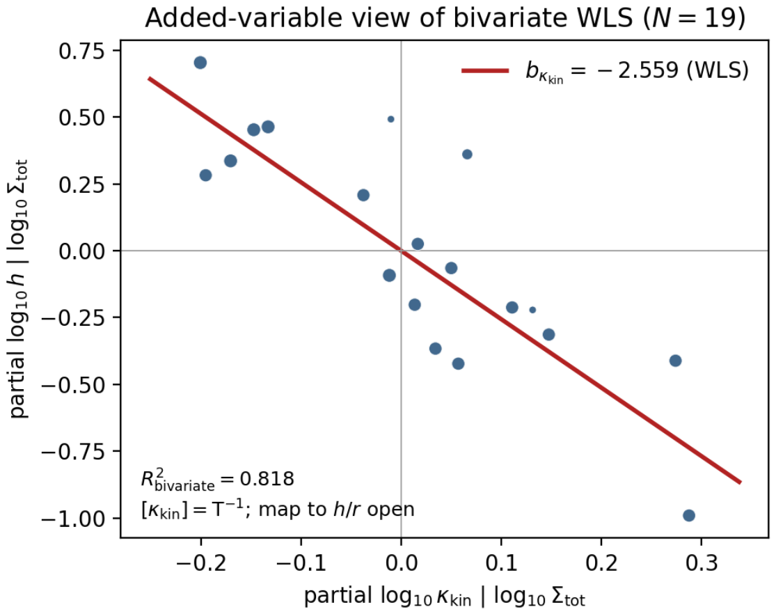
Table 4.
Thickness regression on (, WLS) with frozen bootstrap/LOO robustness. The result is a kinematic–structural association; a map to dimensionless PTQ geometric efficiency remains open.
Table 4.
Thickness regression on (, WLS) with frozen bootstrap/LOO robustness. The result is a kinematic–structural association; a map to dimensionless PTQ geometric efficiency remains open.
| Coefficient | Value | SE | Bootstrap 68% |
|---|---|---|---|
| Intercept a | |||
| (b) | |||
| (c) | |||
| ; AICc; AICc(-only); AICc(-only) | |||
| Bootstrap ; LOO means within SE of full-sample coefficients | |||
Interpretation.
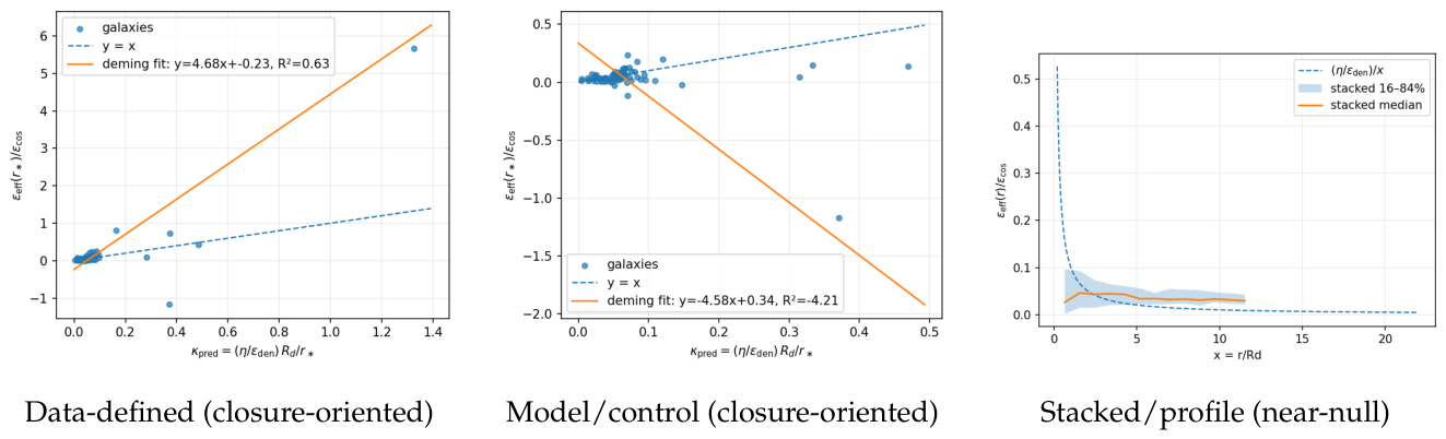
We classify the result as a robust kinematic–structural association whose mapping to a projected-sector geometric efficiency remains open. The coefficient itself is negative and stably so under bootstrap/LOO. Because and the dimensionless aperture are dimensionally inequivalent, a direct sign test of a geometric-efficiency hypothesis is not established by this regression. Additional closure-oriented -like diagnostics (data-defined, model-control, and stacked/profile) use distinct constructions and are reported separately in Appendix B; the stacked/profile control remains near-null ().
4.4. Cross-Scale Consistency Test
Using the adopted map (5) and the PTQ- inference from this study,
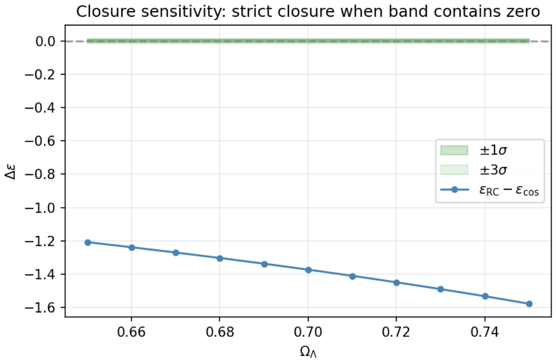
Direct strict equality fails, including throughout a pre-specified -band sensitivity scan under Eqs. (5)–(6). No point in that scan restores equality. The numerical factor required to reconcile the two inferred scales is
In the absence of a validated dimensionless observable bridge, is retained only as a bookkeeping requirement and is not interpreted as evidence for closure. A hypothetical bridge-mediated completion would take the form , where is a dimensionless physical geometric efficiency distinct from the kinematic diagnostic . Such a completion would require a theory-derived or independently motivated definition of , a dimensionally valid observable map, an independent empirical estimate of that quantity, and quantitative agreement with . None of these is established here, so bridge-mediated closure is not yet operationally testable in the present analysis. The failure reported in this section applies to the conjunction of the selected matching relation with the adopted cosmological diagnostic map; it is not a general falsification of complete PTQ.
Figure 2.
Cross-scale closure sensitivity under the adopted diagnostic map. With and , strict cross-scale equality fails, and no point in the pre-specified sensitivity scan restores that equality.
Figure 2.
Cross-scale closure sensitivity under the adopted diagnostic map. With and , strict cross-scale equality fails, and no point in the pre-specified sensitivity scan restores that equality.
5. Discussion
Likelihood analysis, independent structural diagnostic, and cross-scale stress test.
The empirical chain is intentionally staged. Rotation-curve fits determine the likelihood parameters under the full-covariance model. An independent kinematic diagnostic is then compared with external structural information; is not inferred from the PTQ/MOND fit. Cross-scale consistency is tested separately under the selected matching relation and the adopted diagnostic map. Interpretive quantities are therefore not rewarded with additional likelihood freedom.
What SPARC establishes.
Under the present matched full-covariance likelihood, a MOND-like weak-field response describes the data compactly relative to baryons-alone and to the unscreened linear dictionary. Proposition 1 implies that PTQ- and MOND are observationally identical once and the same simple- are imposed, so model-label preference is not evidence for a distinct PTQ radial law. Within the family, does not require a material departure from simple- under AIC. The near-unity best recovered value, together with the absence of AIC support for the additional deformation parameter, makes the response a natural consistency target for future PTQ-specific derivations intended to reproduce this phenomenological branch. Such a derivation should account for why its observable weak-field response remains close to the -like square-root scaling over the acceleration regime probed by SPARC.
What the constrained PTQ interpretation adds.
What the external audits show.
The thickness analysis identifies a robust kinematic–structural association based on , while its mapping to a dimensionless PTQ geometric efficiency remains open. A standard stellar-disk dynamical heuristic provides one possible non-PTQ interpretation of this association [23,24]. For a stellar disk near a common Toomre stability level, links radial velocity dispersion, epicyclic frequency, and surface density [23]; vertical equilibrium likewise links scale height to vertical velocity dispersion and surface density through [24]. If and the velocity-ellipsoid ratio vary only weakly across the relevant subsample, and if the characteristic surface-density proxy tracks the dynamically relevant surface density, these relations schematically imply , i.e. an exponent pair near . The fitted pattern and has the same sign structure and a comparable scale to that simplified relation. Because , , and the exact dynamically relevant surface density are not measured as constant across the sample, and because gas, halo gravity, and radial structure may modify the scaling, we offer this only as an astrophysical hypothesis for the association—not as its explanation, not as a quantitative prediction, and not as evidence for a PTQ geometric mechanism. The classification therefore remains a kinematic–structural association only. Strict selected cosmology-to-galaxy equality fails under the adopted diagnostic map. A bridge-mediated closure remains a future theory target: it would require a dimensionless physical efficiency with an independently defined observable map, whereas the present analysis determines only the numerical factor required for such a reconciliation. These outcomes define concrete targets for future theory work.
Open-source positioning.
The companion repository exposes model equations, parameter accounting, covariance assumptions, fits, deterministic equivalence tests, full-covariance MLE tables, prior-measure statements, geometry diagnostics, closure failure, and a reproducibility record.
6. Conclusion
SPARC discriminates among the tested response architectures under transparent full-covariance accounting, but does not distinguish PTQ- from MOND when the same law and one-to-one matching are adopted. The near-unity recovery makes -like square-root scaling a useful consistency target for future theory intended to reproduce this phenomenological branch. The external structural audit identifies a robust association between disk thickness and the kinematic diagnostic ; a standard disk-dynamical heuristic may qualitatively motivate its sign pattern, while a dimensionally valid map from to a projected-sector geometric efficiency remains open. Strict selected cosmology–galaxy equality fails under the adopted diagnostic map, and a bridge-mediated completion remains observationally and theoretically undefined. Together these results define a constrained observational interface for PTQ-motivated weak-field phenomenology and clear targets for future theory derivation.
Data Availability Statement
SPARC data are publicly available from the SPARC project [9]. Archived analysis artifacts used in this manuscript are distributed with the code repository below.
Acknowledgments
We thank collaborators and maintainers of public SPARC and structural catalogs.
Code availability
Code and figure-generation scripts are openly available at https://github.com/ice91/PTQ-Quaternionic-RC under a permissive license. The immutable release intended for this manuscript is tagged sparc-frontiers-v1.0.0. Reproduction notes are summarized in Appendix F and in the repository file REPRODUCE_PAPER.md.
Appendix A. Diagnostic Notes on κ kin , 〈h/r〉, and the Closure Map
The thickness regression uses the kinematic diagnostic (10) with . The schematic aperture is dimensionless. No frozen map equating to , or to a historical dimensionless PTQ efficiency of the form , is adopted in this manuscript. Historical code filenames containing the token kappa in the geometry archive refer to the kinematic construction used here unless otherwise noted.
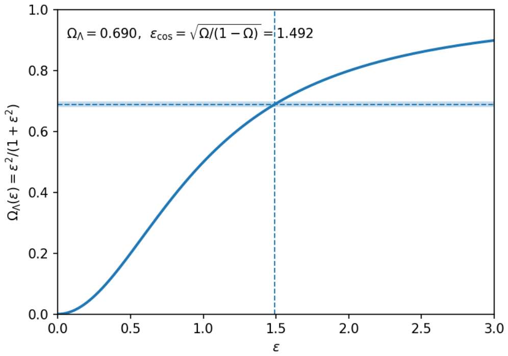
The map (5)–(6) is the adopted diagnostic closure dictionary for the stress test in Sec. Section 4.4; it is not an action-level derivation in the likelihood. Figure A1 visualizes that map alone.
Figure A1.
Adopted diagnostic dictionary used in the closure stress test. The curve visualizes the chosen map; it is not presented as a derived PTQ cosmological prediction from SPARC.
Figure A1.
Adopted diagnostic dictionary used in the closure stress test. The curve visualizes the chosen map; it is not presented as a derived PTQ cosmological prediction from SPARC.
Appendix B. Distinct Closure-Oriented κ-like Diagnostics
The following panels use constructions distinct from the kinematic thickness diagnostic (Sec. Section 4.3). They are retained as triangulation of mixed geometry/closure-oriented evidence and are not presented as the same observable.
Figure A2.
Mixed -like diagnostics distinct from . Positive/unstable/near-null patterns coexist; none of these panels is identified with the thickness-regression predictor, and none confirms a geometric interception mechanism.
Figure A2.
Mixed -like diagnostics distinct from . Positive/unstable/near-null patterns coexist; none of these panels is identified with the thickness-regression predictor, and none confirms a geometric interception mechanism.
Appendix C. Shared Simple-ν Residual Phenomenology
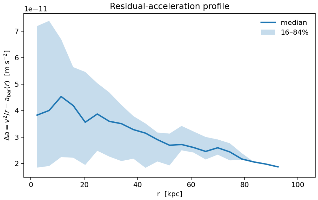
Under the adopted simple- response, outer-disk residuals exhibit a shared plateau-like phenomenology across the SPARC sample. Figure A3 is retained as a visualization of that common MOND-like weak-field behavior. It is not interpreted as a PTQ-specific signature, nor as independent confirmation of the thickness association.
Figure A3.
Shared simple- residual / plateau phenomenology on the SPARC sample. The feature is treated as common MOND-like weak-field behavior under the adopted response, not as a PTQ-specific signature.
Figure A3.
Shared simple- residual / plateau phenomenology on the SPARC sample. The feature is treated as common MOND-like weak-field behavior under the adopted response, not as a PTQ-specific signature.
Appendix D. Near-Null Stacked/Profile Diagnostic
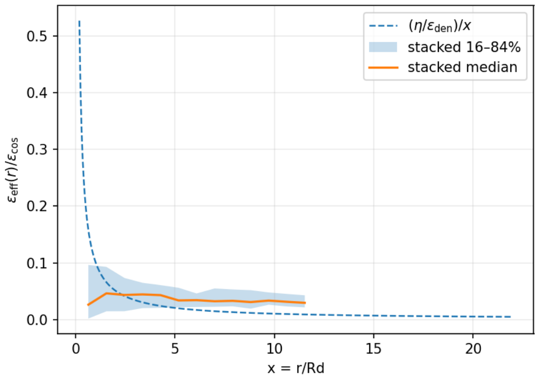
The stacked/profile geometry diagnostic remains near-null (). Figure A4 isolates that negative control so that it is not hidden behind the thickness association.
Figure A4.
Standalone stacked/profile geometry diagnostic (near-null; ). This negative control is retained explicitly and is not hidden behind the thickness association.
Figure A4.
Standalone stacked/profile geometry diagnostic (near-null; ). This negative control is retained explicitly and is not hidden behind the thickness association.
Appendix E. Legacy Diagonalized Predictive Scores
Archived WAIC/PSIS-LOO tables in the repository evaluate pointwise contributions using diagonalized per-radius variance terms while the primary fits use full . They are sensitivity diagnostics for reproducibility of the legacy Bayesian analysis and must not be read as canonical full-covariance predictive rankings of distinct radial laws. Multi-seed WAIC tables, when present, document reproducibility of that sensitivity analysis only. NFW scores in that construction are not used for headline ranking. These radius-level predictive scores are distinct from the galaxy-level leave-one-out checks of the thickness regression in Sec. Section 4.3.
Appendix F. Reproducibility Sketch
Canonical import path: PYTHONPATH=$IMPL_ROOT/src. Machine-readable numerical results include the paper-submission archive under results/paper_submission_ptqnu_20260323/ and the full-covariance MLE tables under results/scientific_hardening_r1/01_mle/. Figure files used in this manuscript are copied from those archives without regeneration, except for the deterministic added-variable re-rendering of the frozen WLS regression used as Figure 1.
References
- Chen, C.-C. Guaranteed Tensor Luminality from Symmetry: A PT-Even Palatini Torsion Framework. Symmetry 2026, 18, 170. [Google Scholar] [CrossRef]
- B. P. Abbott et al. (LIGO Scientific Collaboration and Virgo Collaboration); et al. GW170817: Observation of Gravitational Waves from a Binary Neutron Star Inspiral. Phys. Rev. Lett. 2017, 119, 161101. [Google Scholar] [CrossRef] [PubMed]
- Abbott, B. P.; et al. Multi-messenger Observations of a Binary Neutron Star Merger. Astrophys. J. Lett. 2017, 848, L12. [Google Scholar] [CrossRef]
- Tully, R. B.; Fisher, J. R. A new method of determining distances to galaxies. Astron. Astrophys. 1977, 54, 661–673. [Google Scholar]
- Milgrom, M. A modification of the Newtonian dynamics: Implications for galaxies. Astrophys. J. 1983, 270, 365–370. [Google Scholar] [CrossRef]
- McGaugh, S. S. The Baryonic Tully–Fisher Relation of Galaxies with Extended Rotation Curves and the Stellar Mass of Rotating Galaxies. Astrophys. J. 2005, 632, 859–871. [Google Scholar] [CrossRef] [PubMed]
- Famaey, B.; McGaugh, S. Modified Newtonian Dynamics (MOND): Observational Phenomenology and Relativistic Extensions. Living Rev. Relativ. 2012, 15, 10. [Google Scholar] [CrossRef] [PubMed]
- McGaugh, S. S.; Lelli, F.; Schombert, J. M. Radial Acceleration Relation in Rotationally Supported Galaxies. Phys. Rev. Lett. 2016, 117, 201101. [Google Scholar] [CrossRef] [PubMed]
- Lelli, F.; McGaugh, S. S.; Schombert, J. M. SPARC: Mass models for 175 disk galaxies with Spitzer photometry and accurate rotation curves. Astron. J. 2016, 152, 157. [Google Scholar] [CrossRef]
- Sheth, K.; et al. The Spitzer Survey of Stellar Structure in Galaxies (S4G). Publ. Astron. Soc. Pac. 2010, 122, 1397. [Google Scholar] [CrossRef]
- Meidt, S. E.; et al. Reconstructing the Stellar Mass Distributions of Galaxies Using S4G IRAC 3.6 and 4.5 μm Images. II. The Conversion from Light to Mass. Astrophys. J. 2014, 788, 144. [Google Scholar] [CrossRef]
- Díaz-García, A. M.; Salo, J. C.; Laurikainen, H.; Athanassoula, E. Global stellar-to-halo mass relation and the role of bars in S4G. Astron. Astrophys. 2016, 587, A160. [Google Scholar] [CrossRef]
- Navarro, J. F.; Frenk, C. S.; White, S. D. M. A Universal Density Profile from Hierarchical Clustering. Astrophys. J. 1997, 490, 493–508. [Google Scholar] [CrossRef] [PubMed]
- Dutton, A. A.; Macciò, A. V. Cold dark matter haloes in the Planck era: evolution of density profiles and concentration–mass relation. Mon. Not. R. Astron. Soc. 2014, 441, 3359–3374. [Google Scholar] [CrossRef]
- Akaike, H. A new look at the statistical model identification. IEEE Trans. Autom. Control 1974, 19, 716–723. [Google Scholar] [CrossRef]
- Schwarz, G. Estimating the dimension of a model. Ann. Stat. 1978, 6, 461–464. [Google Scholar] [CrossRef]
- Sugiura, N. Further analysis of the data by Akaike’s information criterion and the finite corrections. Commun. Stat. Theory Methods 1978, 7, 13–26. [Google Scholar] [CrossRef]
- Hurvich, C. M.; Tsai, C. L. Regression and time series model selection in small samples. Biometrika 1989, 76, 297–307. [Google Scholar] [CrossRef]
- Creminelli, P.; Vernizzi, F. Dark Energy after GW170817 and GRB170817A. Phys. Rev. Lett. 2017, 119, 251302. [Google Scholar] [CrossRef] [PubMed]
- Ezquiaga, J. M.; Zumalacárregui, M. Dark Energy After GW170817: Dead Ends and the Road Ahead. Phys. Rev. Lett. 2017, 119, 251304. [Google Scholar] [CrossRef] [PubMed]
- Baker, T.; Bellini, E.; Ferreira, P. G.; Lagos, M.; Noller, J.; Sawicki, I. Strong Constraints on Cosmological Gravity from GW170817 and GRB 170817A. Phys. Rev. Lett. 2017, 119, 251301. [Google Scholar] [CrossRef] [PubMed]
- Planck Collaboration: N. Aghanim et al., Planck 2018 results. VI. Cosmological parameters. Astron. Astrophys. 2020, 641, A6. [CrossRef]
- Toomre, A. On the gravitational stability of a disk of stars. Astrophys. J. 1964, 139, 1217–1238. [Google Scholar] [CrossRef]
- van der Kruit, P. C.; Freeman, K. C. Galaxy disks. Annu. Rev. Astron. Astrophys. 2011, 49, 301–371. [Google Scholar] [CrossRef]
- Chen, C.-C. “Projection-Defined Physicality in PT-Symmetric Quaternionic Spacetime,” Preprints.org; 2026. [Google Scholar] [CrossRef]
- Chen, C.-C. PT-Projected Projective Palatini Gravity: Two-Derivative Operator Basis, Admissible Equivalences, and a Local IR Residual. Preprints.org 2026. [Google Scholar] [CrossRef]
- Chen, C.-C. “A Conditional Scalar-Gradient Trace-Torsion Branch in PT-Even Einstein–Cartan Geometry,” Preprints.org; 2026. [Google Scholar] [CrossRef]
Table 1.
SPARC sample flow used in this study. The final cuts are applied as a single combined quality query after merge/dropna.
Table 1.
SPARC sample flow used in this study. The final cuts are applied as a single combined quality query after merge/dropna.
| Stage | ||
|---|---|---|
| SPARC Table 1 galaxies | 175 | — |
| SPARC Table 2 rotation-curve points | 175 | 3391 |
| After merge + dropna | 175 | 3391 |
| After combined quality cuts | 91 | 1782 |
Table 3.
Full-covariance MLE accounting (, ). AIC . uses by convention. For NFW-1p we report the best recovered full-covariance likelihood in the present multistart search; cross-start scatter is and is not hidden.
Table 3.
Full-covariance MLE accounting (, ). AIC . uses by convention. For NFW-1p we report the best recovered full-covariance likelihood in the present multistart search; cross-start scatter is and is not hidden.
| Model | k | AIC | ||
|---|---|---|---|---|
| NFW-1p | 183 | |||
| MOND = PTQ- | 93 | |||
| family | 94 | |||
| PTQ linear | 93 | |||
| Baryon | 92 |
Disclaimer/Publisher’s Note: The statements, opinions and data contained in all publications are solely those of the individual author(s) and contributor(s) and not of MDPI and/or the editor(s). MDPI and/or the editor(s) disclaim responsibility for any injury to people or property resulting from any ideas, methods, instructions or products referred to in the content. |
© 2026 by the authors. Licensee MDPI, Basel, Switzerland. This article is an open access article distributed under the terms and conditions of the Creative Commons Attribution (CC BY) license (http://creativecommons.org/licenses/by/4.0/).
Copyright: This open access article is published under a Creative Commons CC BY 4.0 license, which permit the free download, distribution, and reuse, provided that the author and preprint are cited in any reuse.


