Submitted:
25 March 2025
Posted:
27 March 2025
Read the latest preprint version here
Abstract
Keywords:
1. What Is Exploratory Spatial Data Analysis (ESDA)
2. Basic Univariate ESDA
2.1. For Continuous Variables
2.1.1. Histogram
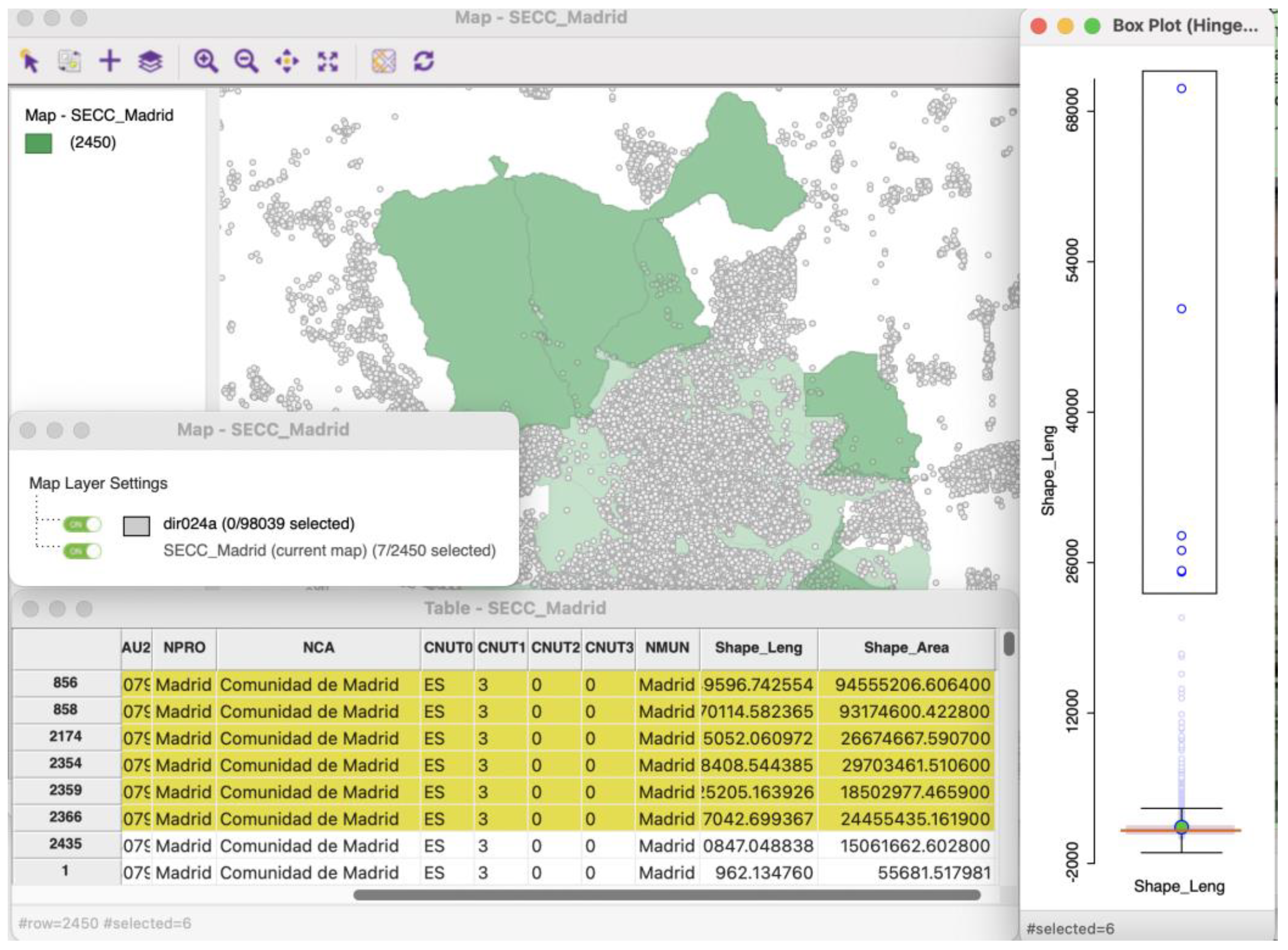
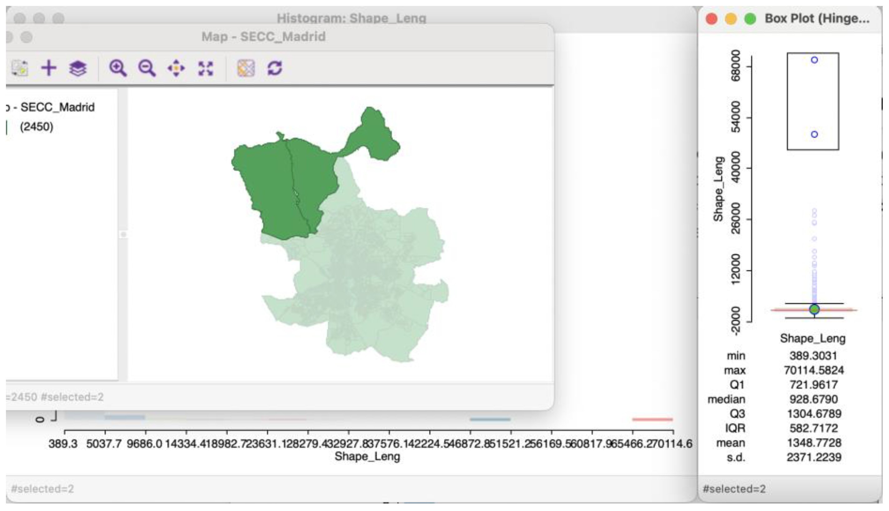
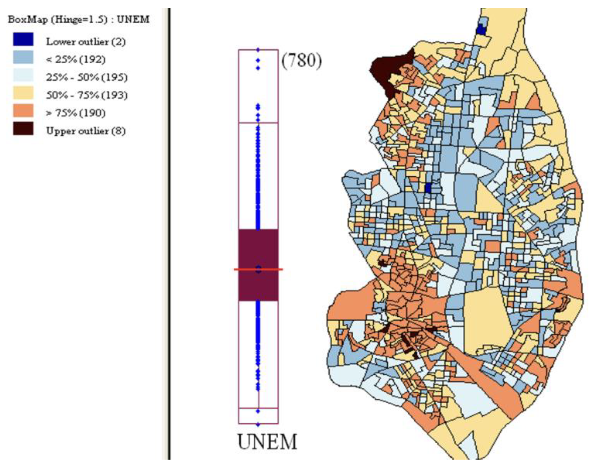
2.1.2. Box Plot
2.1.3. Thematic Maps
- 1)
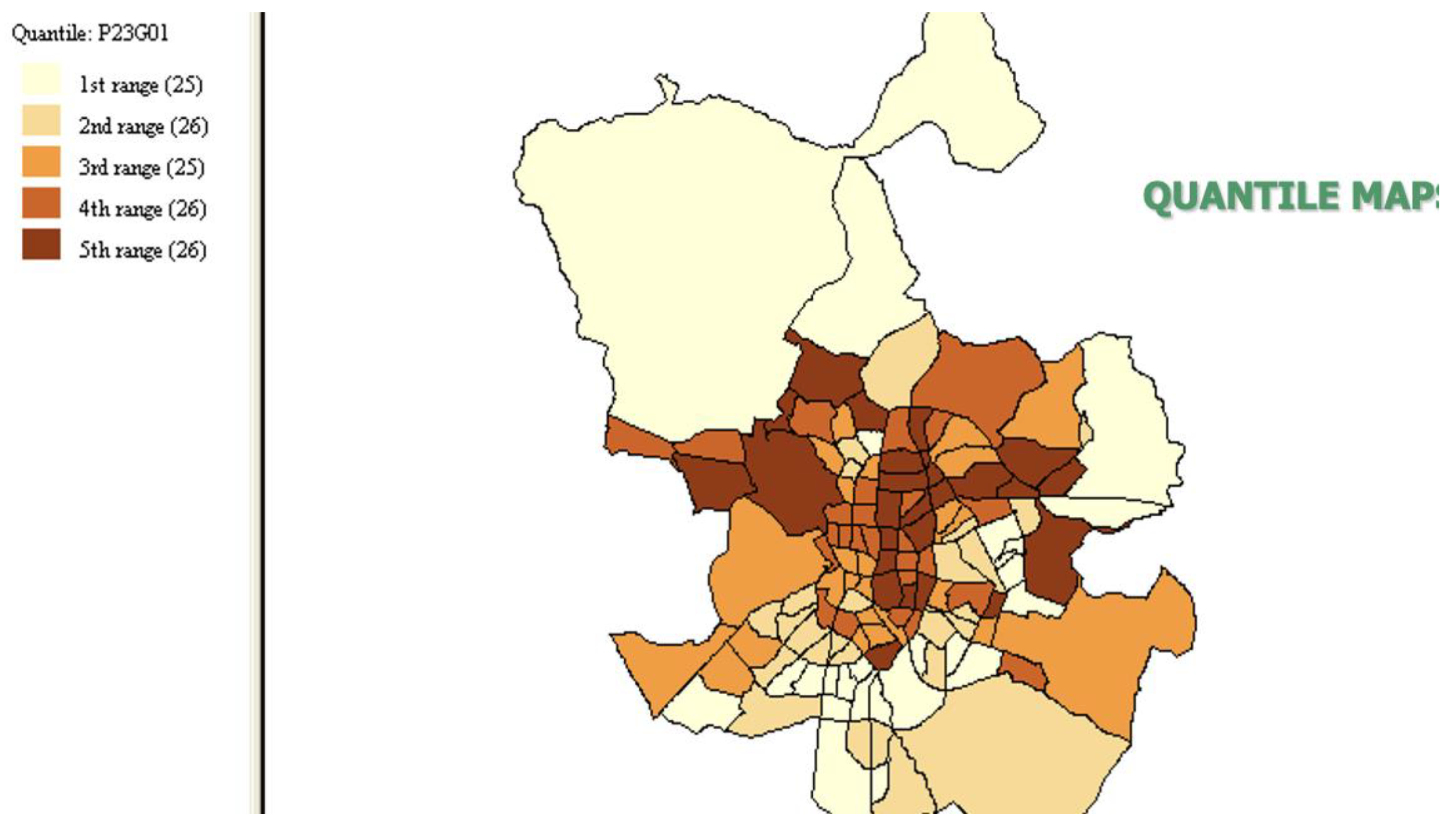
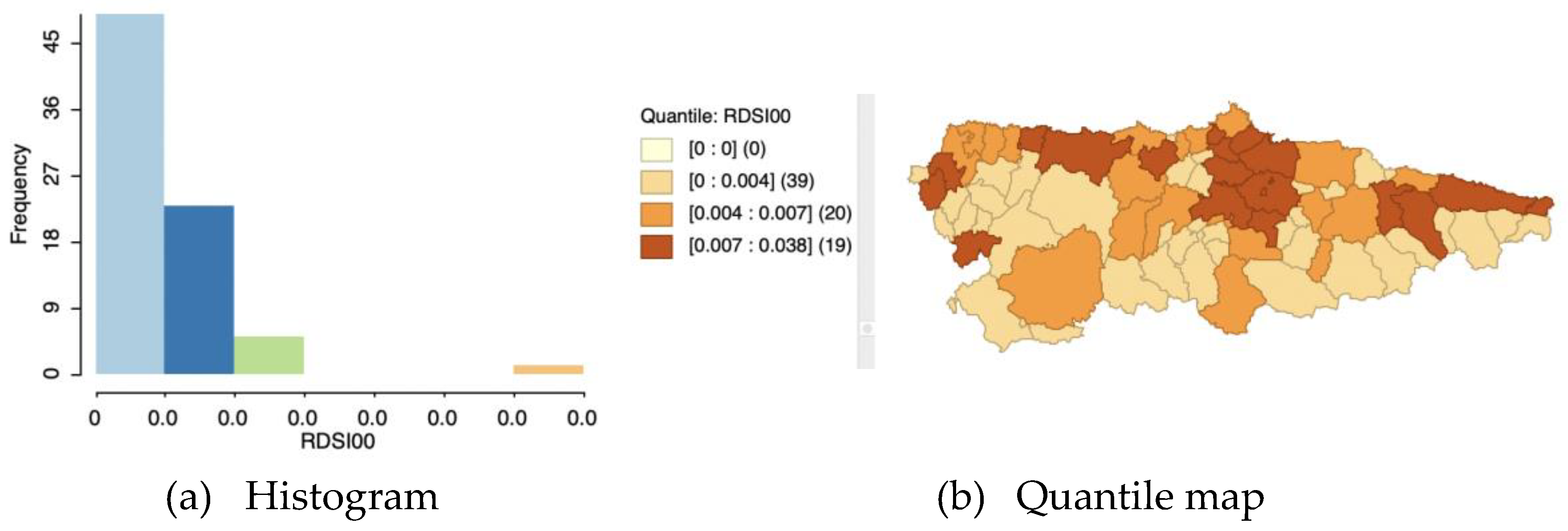
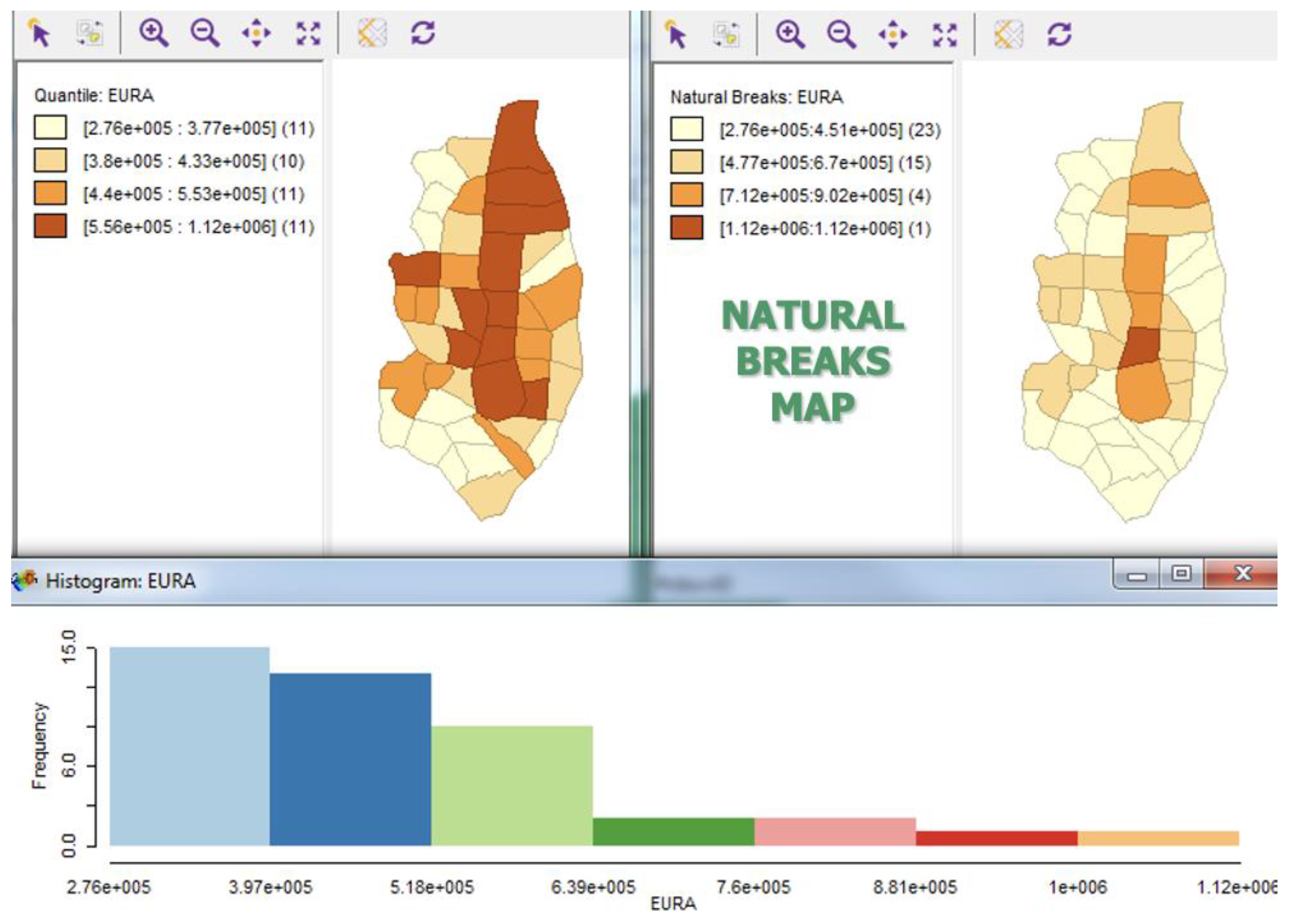
- Quantile map
- 2)
- Natural breaks map
- 3)
- Box map
2.2. For Discrete Variables
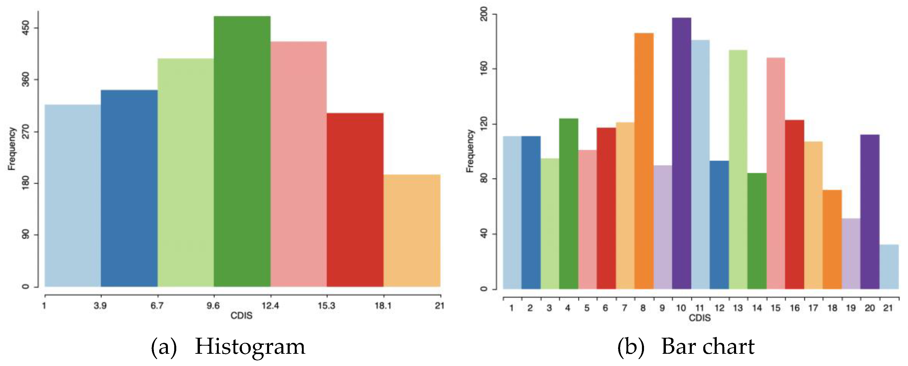
2.2.1. Bar Chart
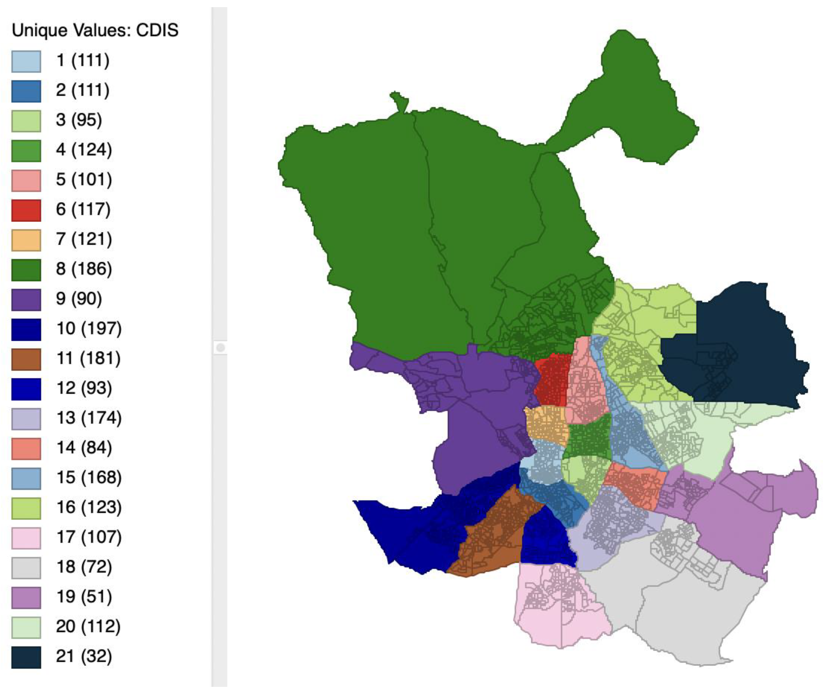
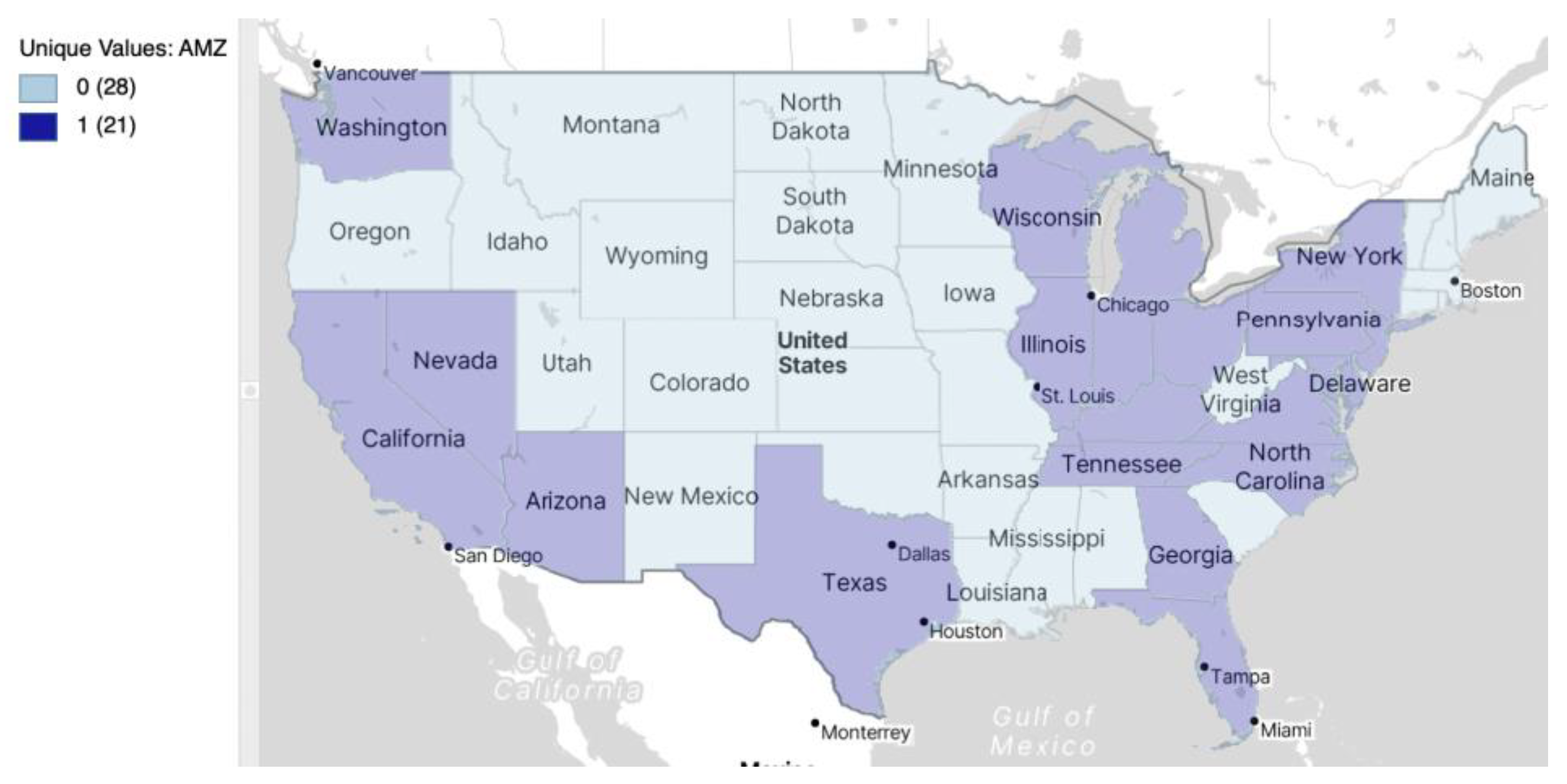
2.2.2. Unique Values Map
2.3. Map Classification, Legends and Colors
- a)
- For maps where the values represented are ordered and follow a single direction, from low to high, a sequential legend is appropriate. Such a legend typically uses a single tone and associates higher categories with increasingly darker values.
- b)
- In contrast, for the maps representing the extreme values of a variable, the focus should be on the central tendency (mean or median) and how observations sort themselves away from the center, either in downward or upward direction. An appropriate legend for this situation is a diverging legend, which emphasizes the extremes in either direction. It uses two different tones, one for the downward direction (typically blue) and one for the upward direction (typically red or brown).
- c)
- Finally, for categorical data a qualitative legend is appropriate; that is, no order should be implied (no high or low values) and the legend should suggest the equivalence of categories.
3. Basic Multivariate ESDA
3.1. For Continuous Variables
3.1.1. Scatter Plot
- 1)
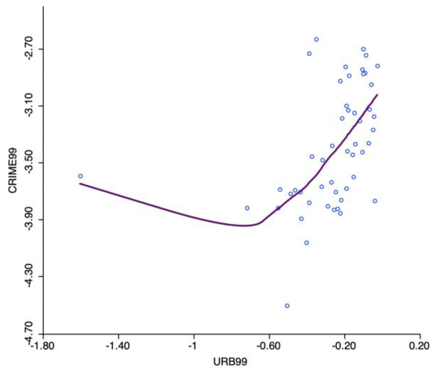
- Non-linear relationships
- -
- The bandwidth is the proportion of points in the plot that influence smoothing at each value, so as larger values give more smoothness. For example, the default bandwidth of 0.20 implies that for each local fit (centered on a value for X), about one fifth of the range of X-values is considered.
- -
- Iterations: are the number of “robustifying” iterations which should be performed. Using smaller values will speed up the smoothing.
- -
- Delta factor: Small values of delta speed up computation because local polynomial fit is only computed for a small amount of data at each data point, filling in the fitted values for the skipped points with linear interpolation.
- 2)
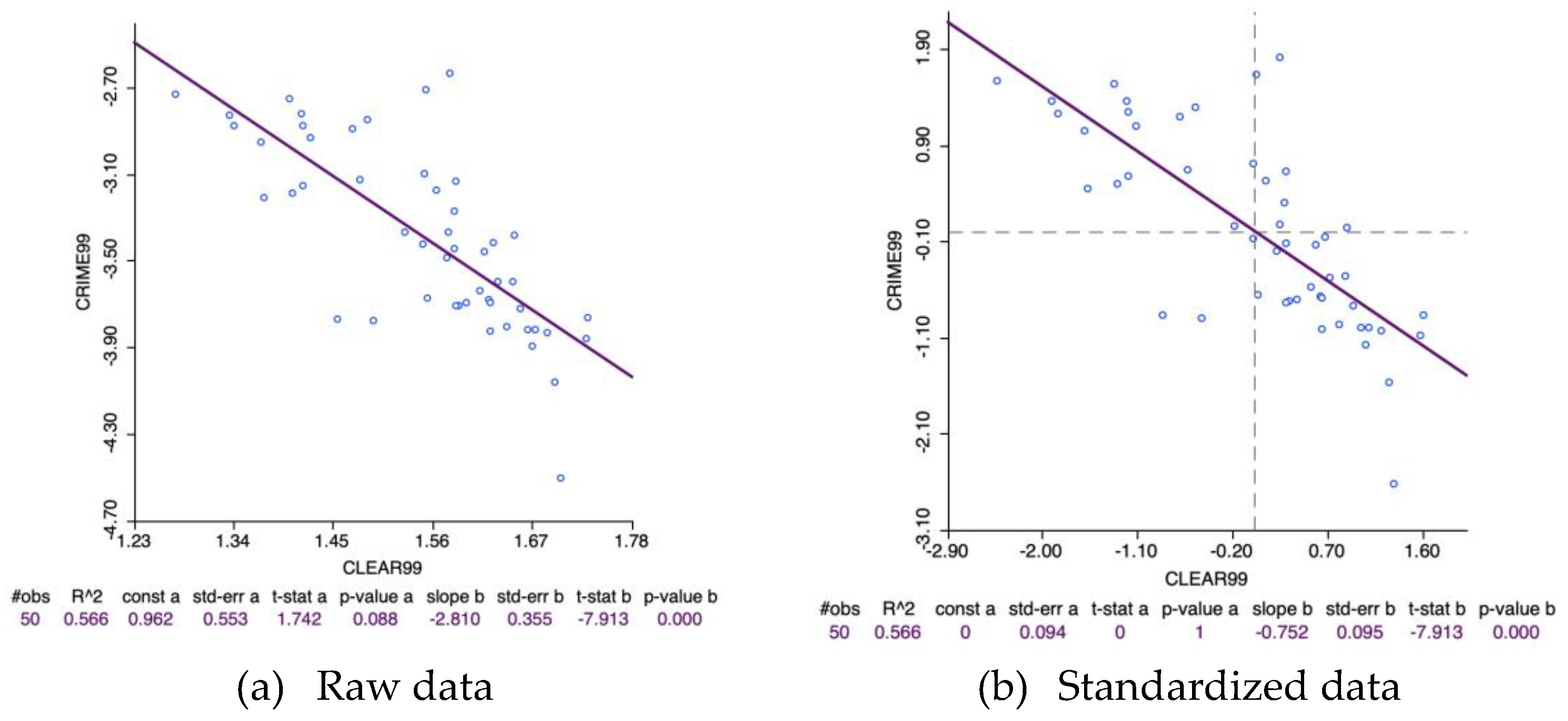
- Standardization of the x, y variables
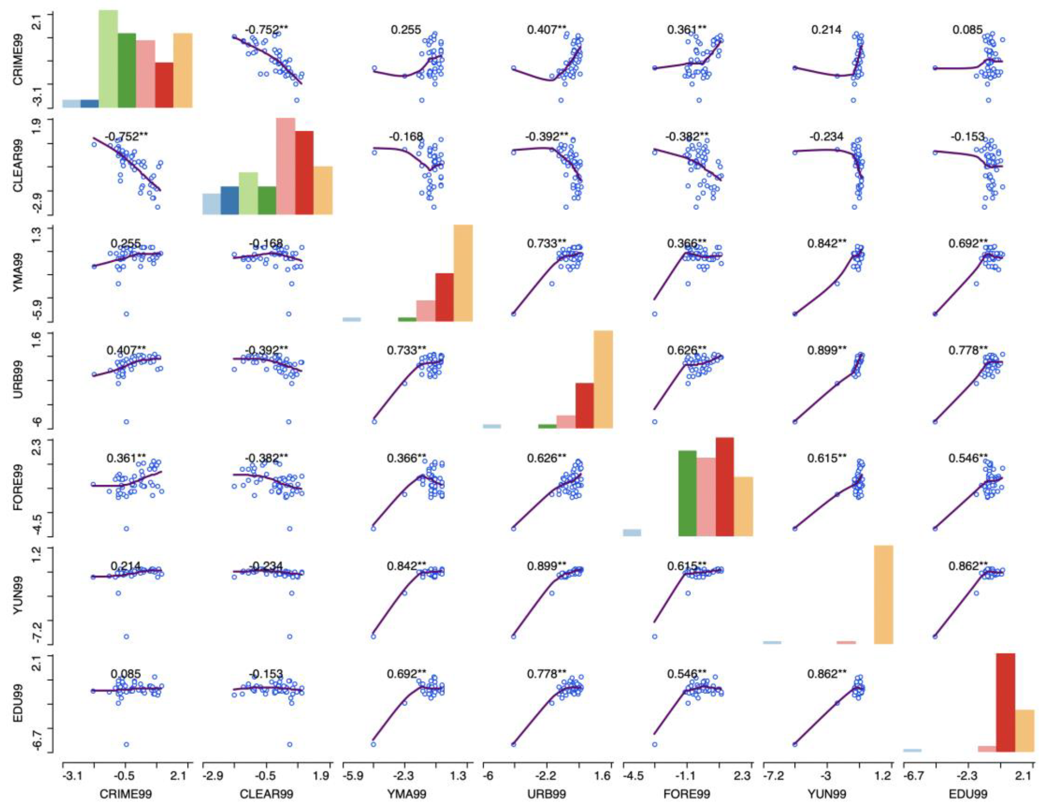
3.1.2. Scatter Plot Matrix
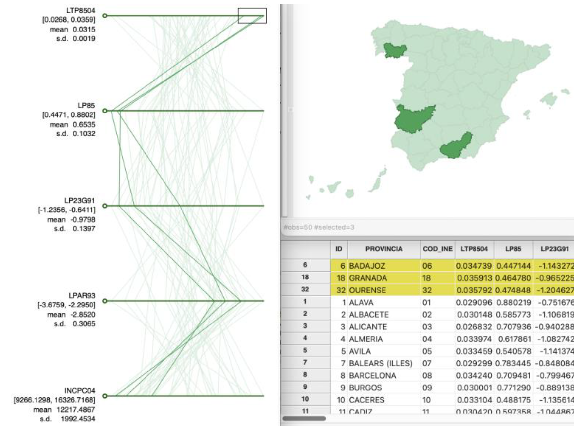
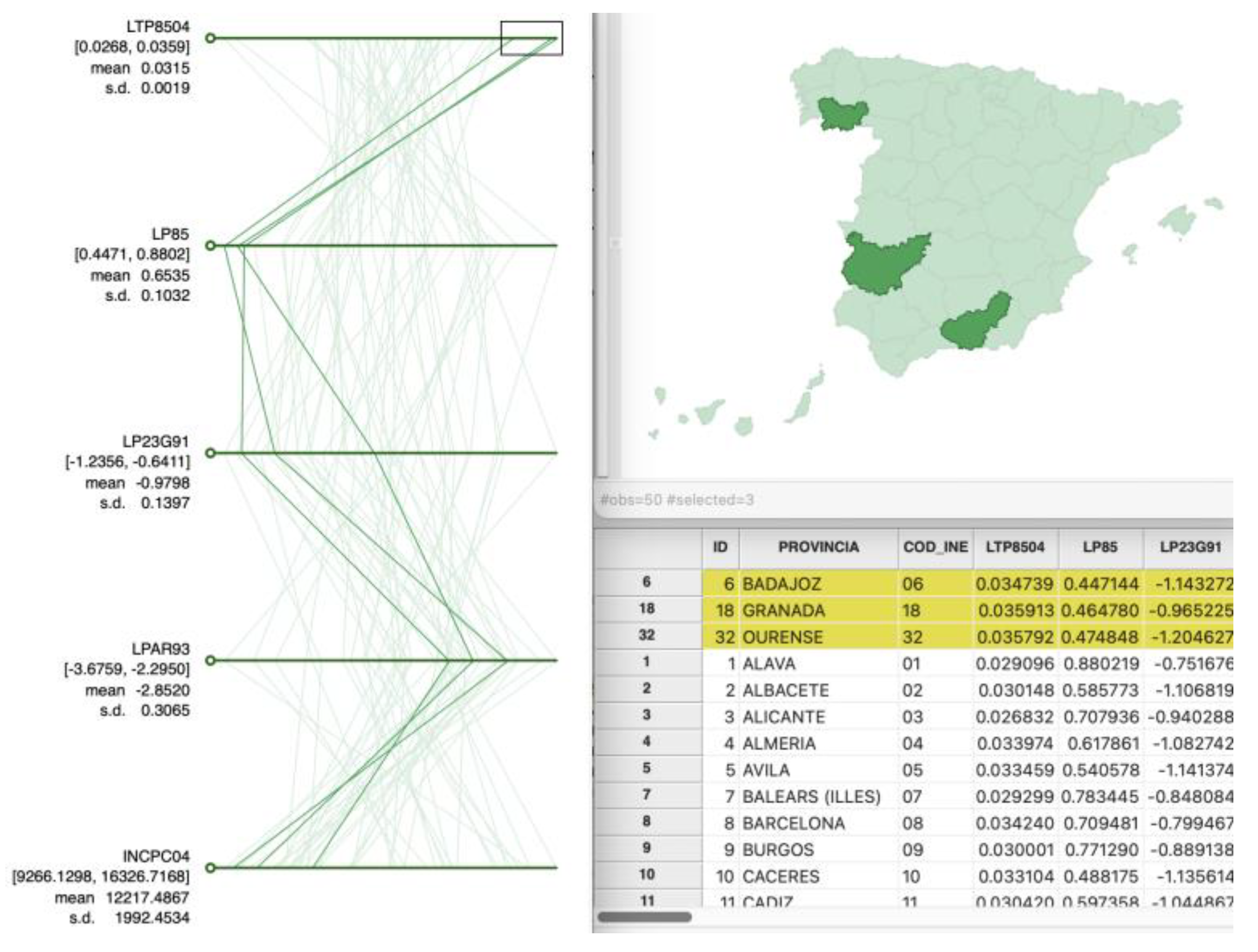
3.1.3. Parallel Coordinate Plot
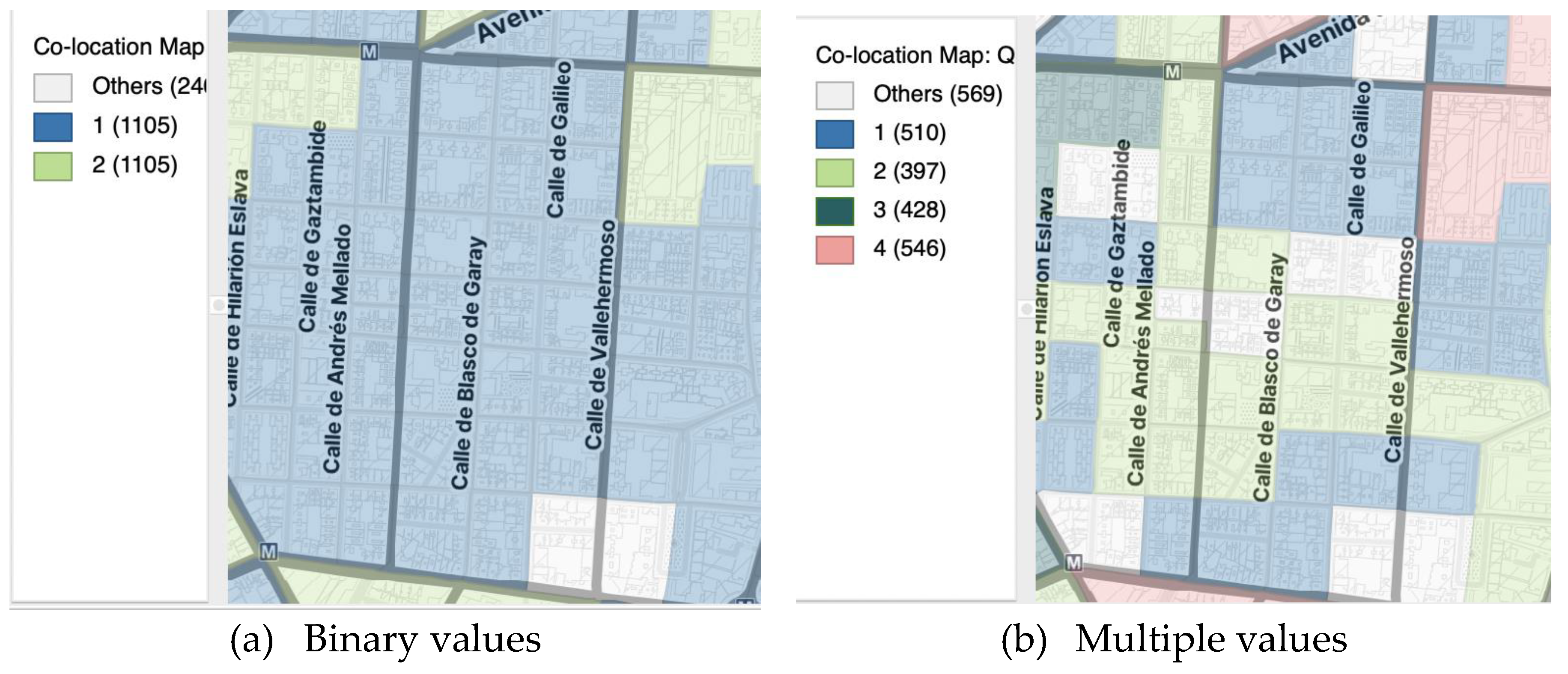
3.2. For Discrete Data: Co-Location Map
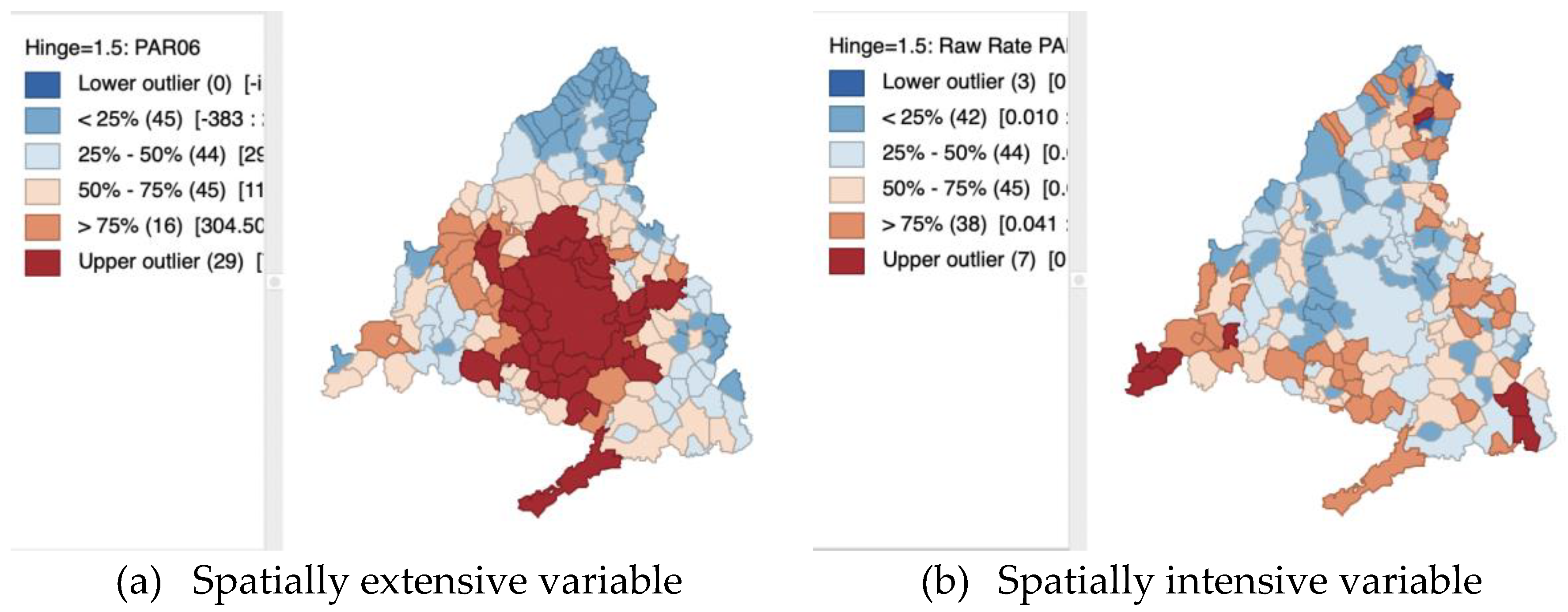
3.3. For Rates or Proportions
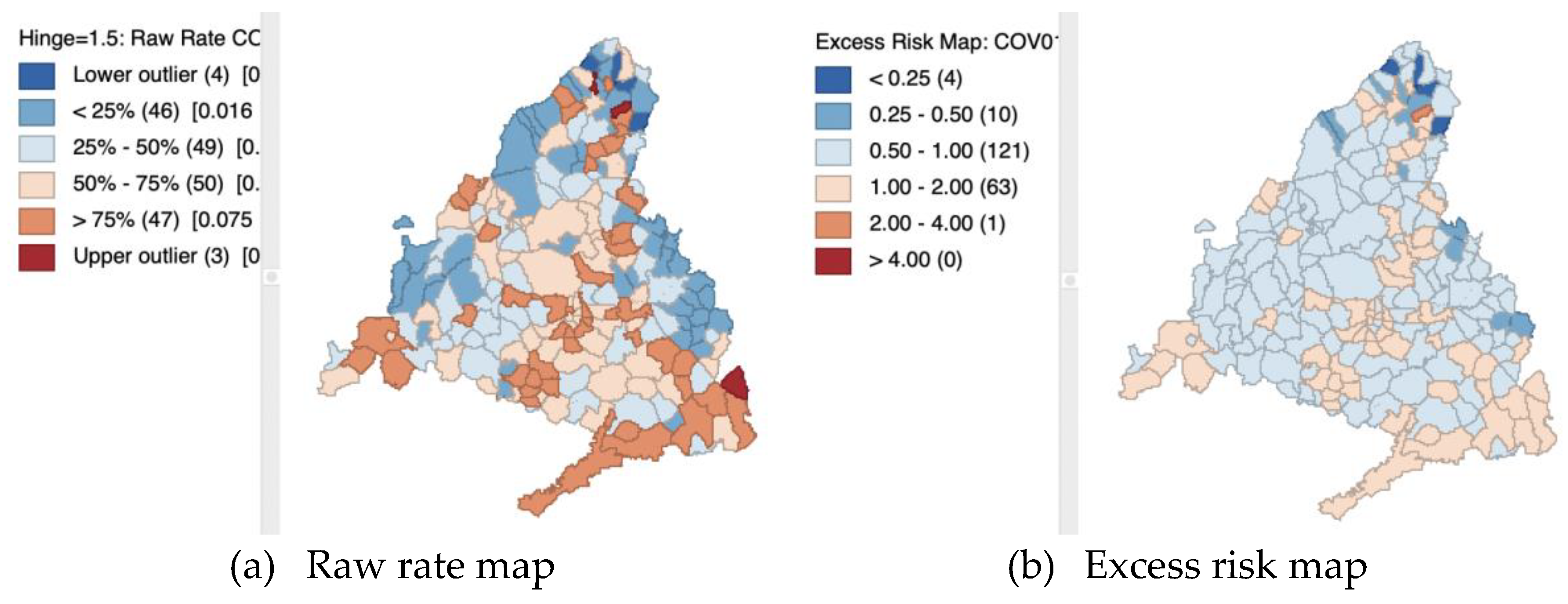
3.3.1. Raw Rate Map
3.3.2. Relative Risk or Rate
3.3.3. Excess Risk Map
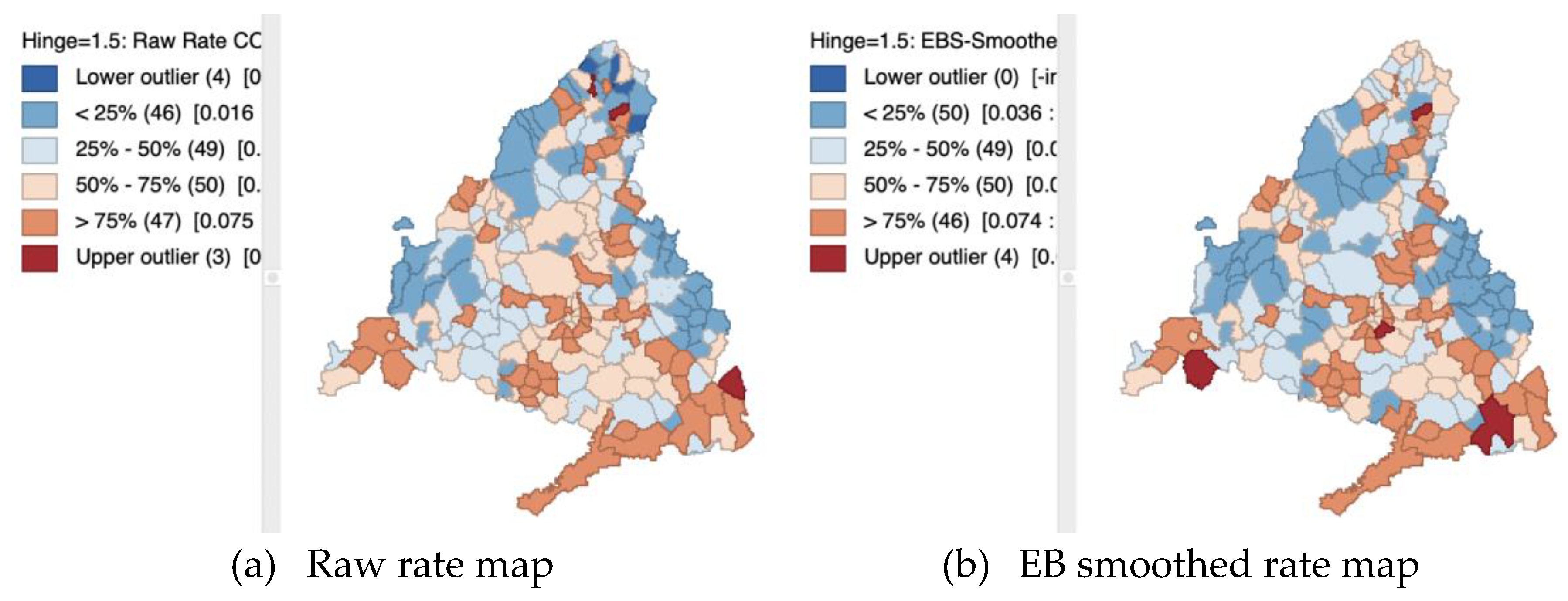
3.3.4. Empirical Bayes Smoothed Rate Map
3.4. For Space-Time Data
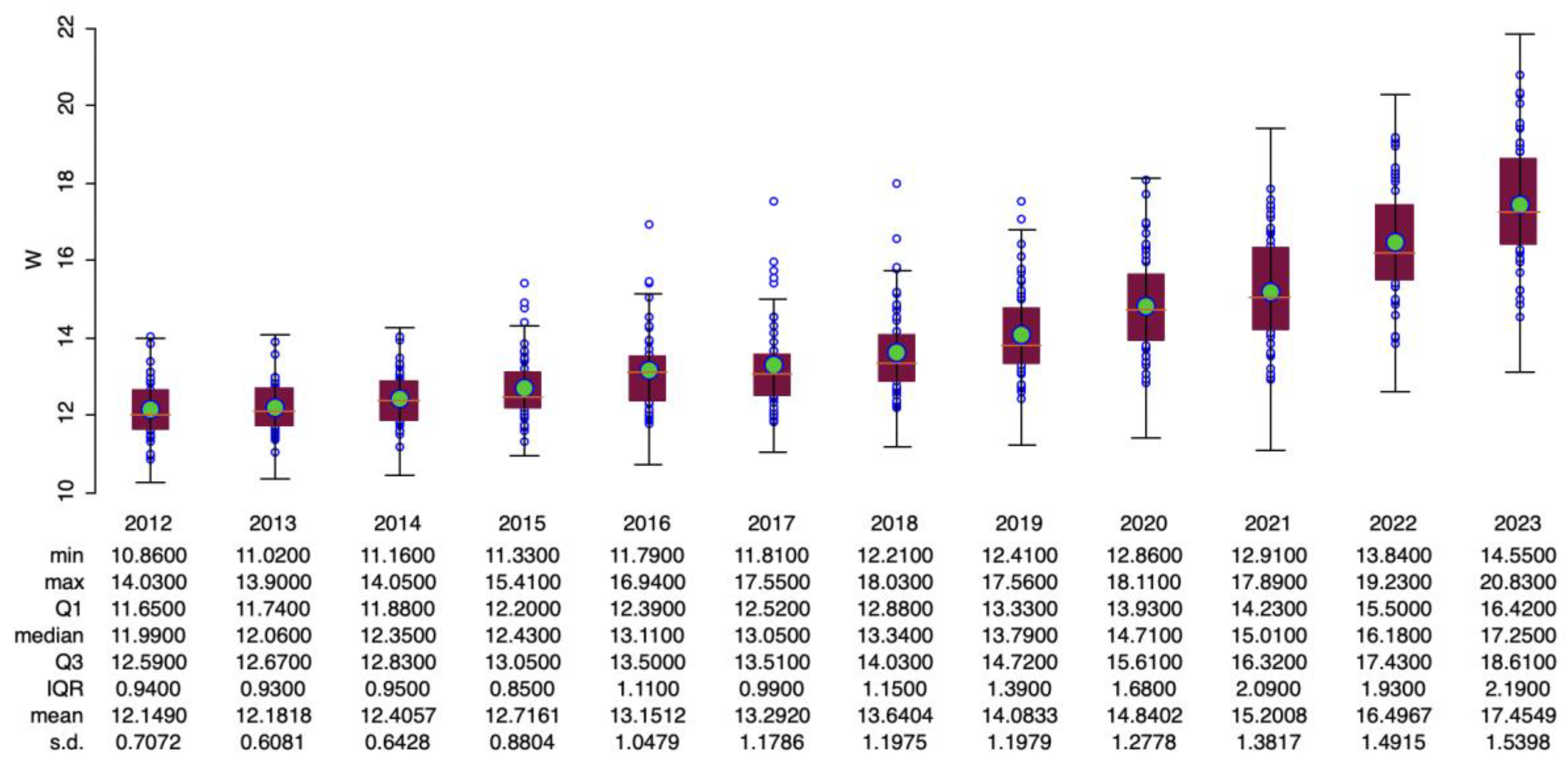
3.4.1. Space-Time Box Plot
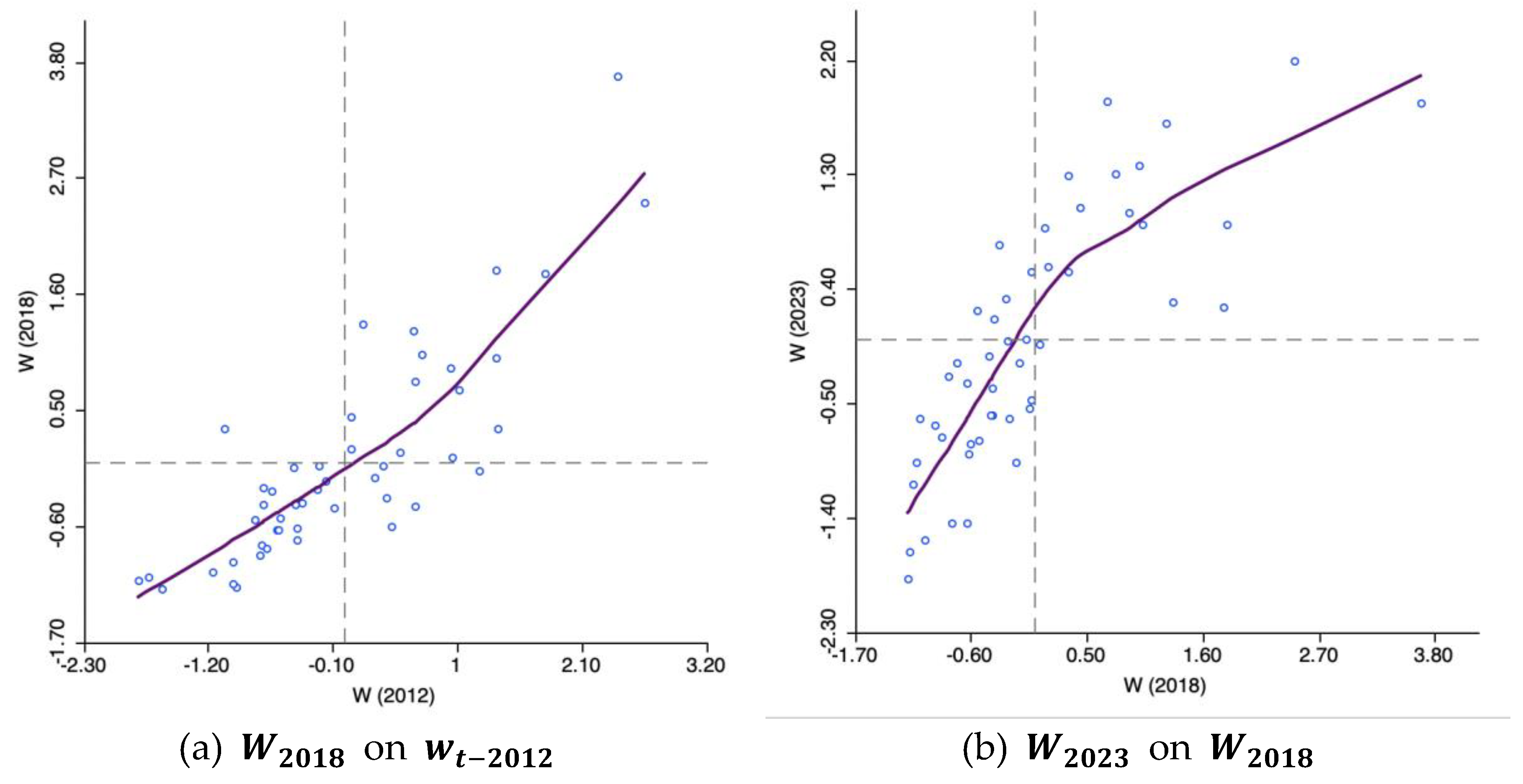
3.4.2. Time-Wise Autoregressive Scatter Plot
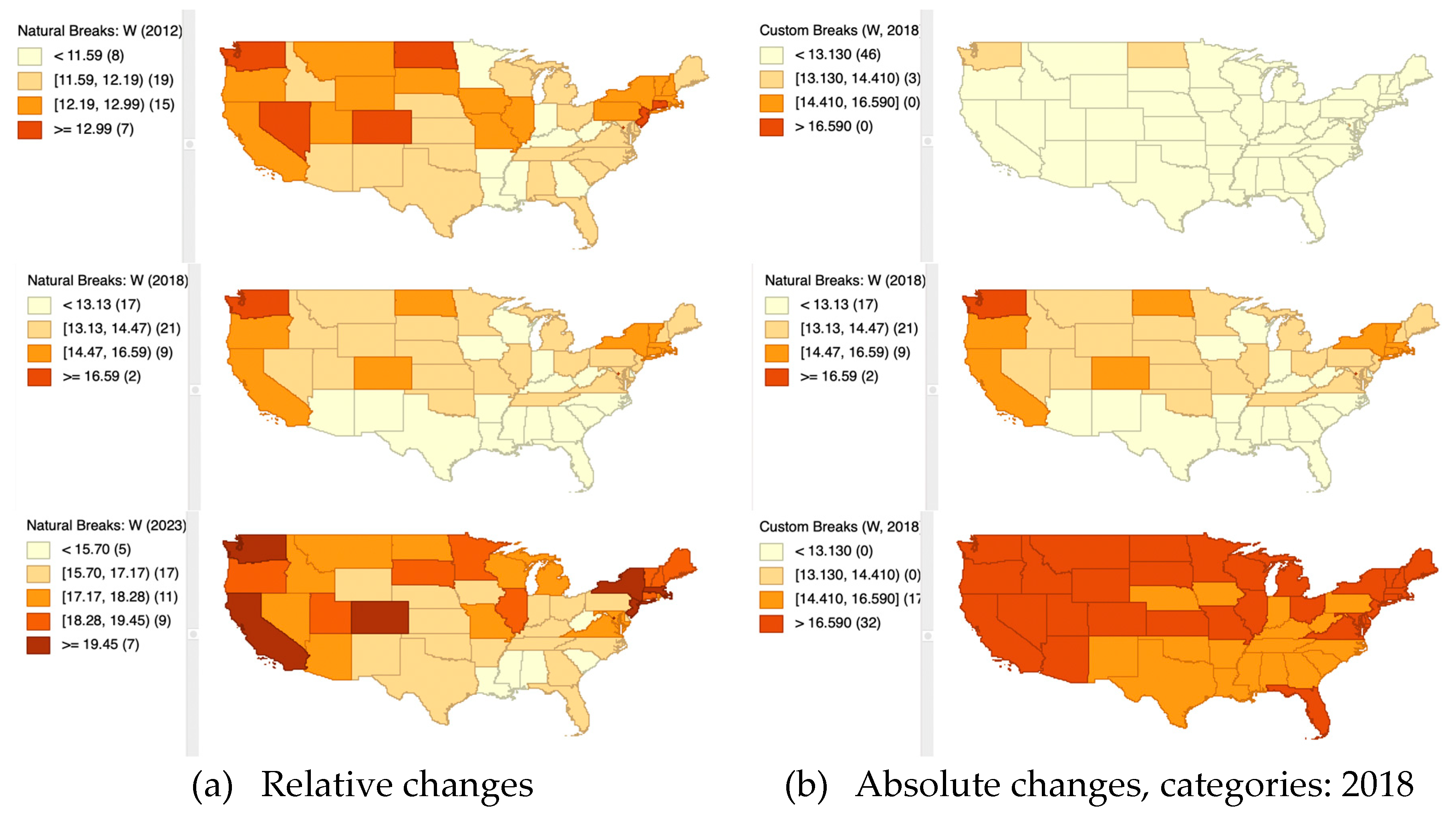
3.4.3. Space-Time Choropleth Map
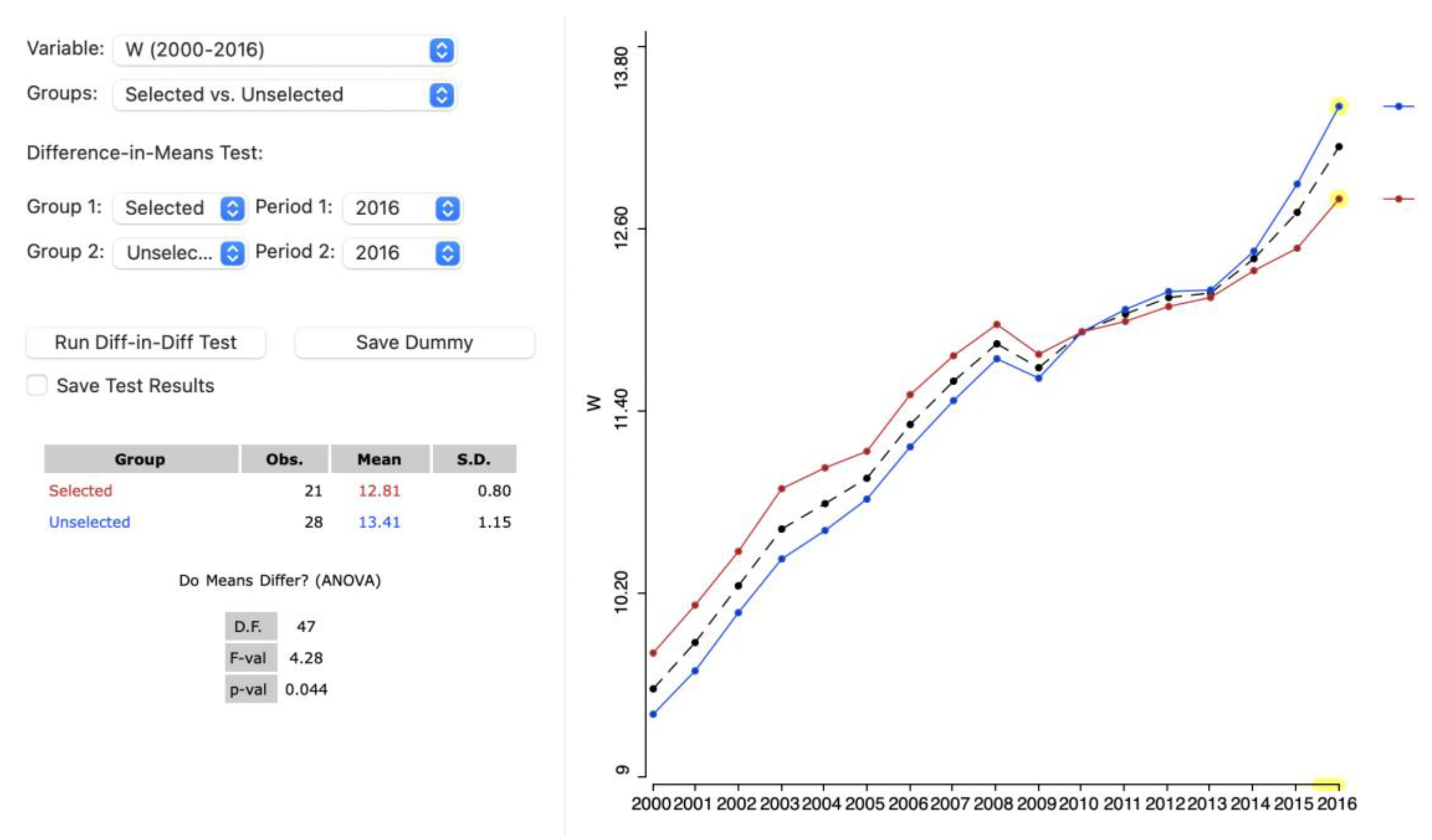
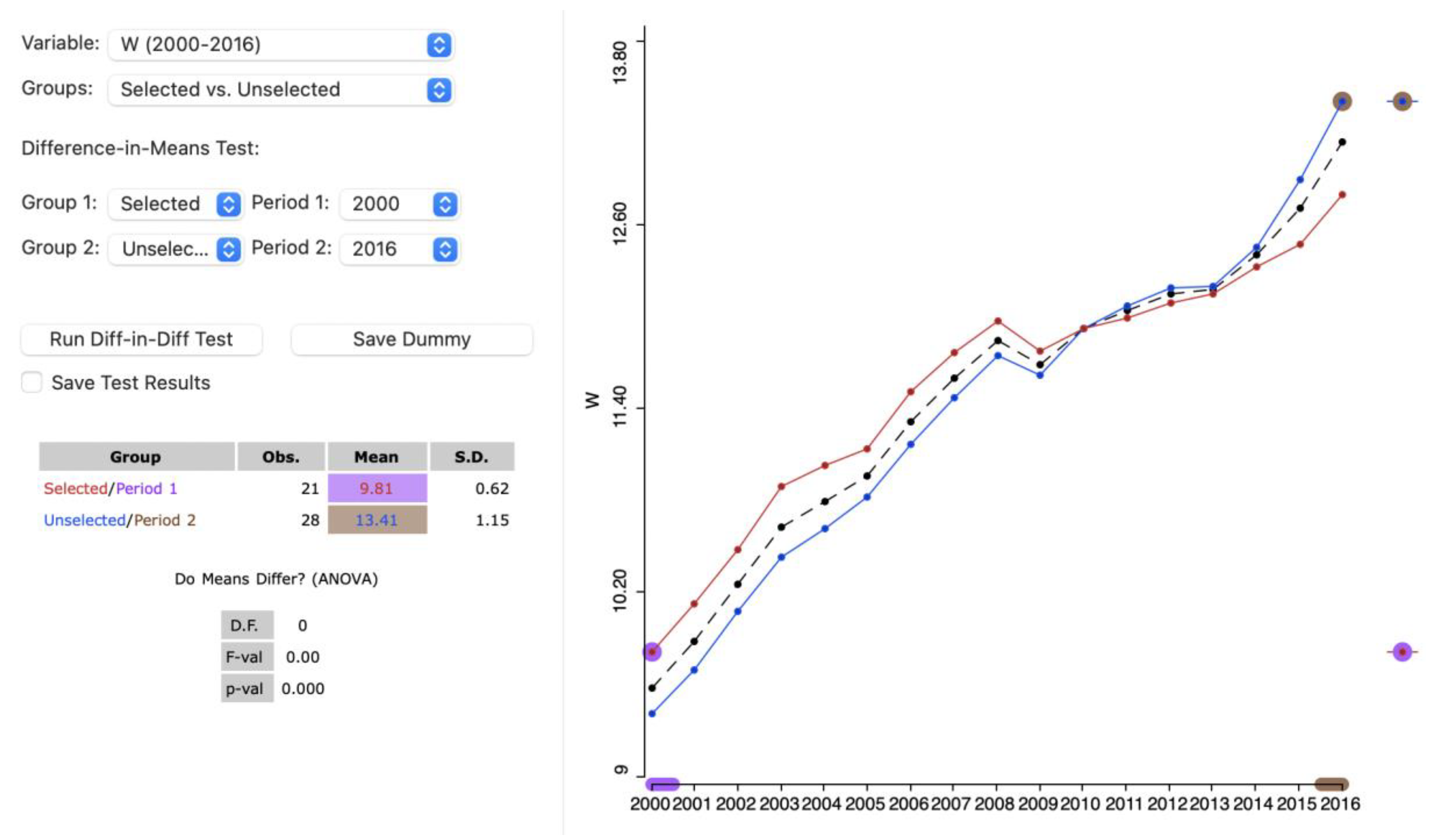
3.4.4. Treatment Effect Analysis: Averages Chart
- 1)
- Difference-in-Means test
- 2)
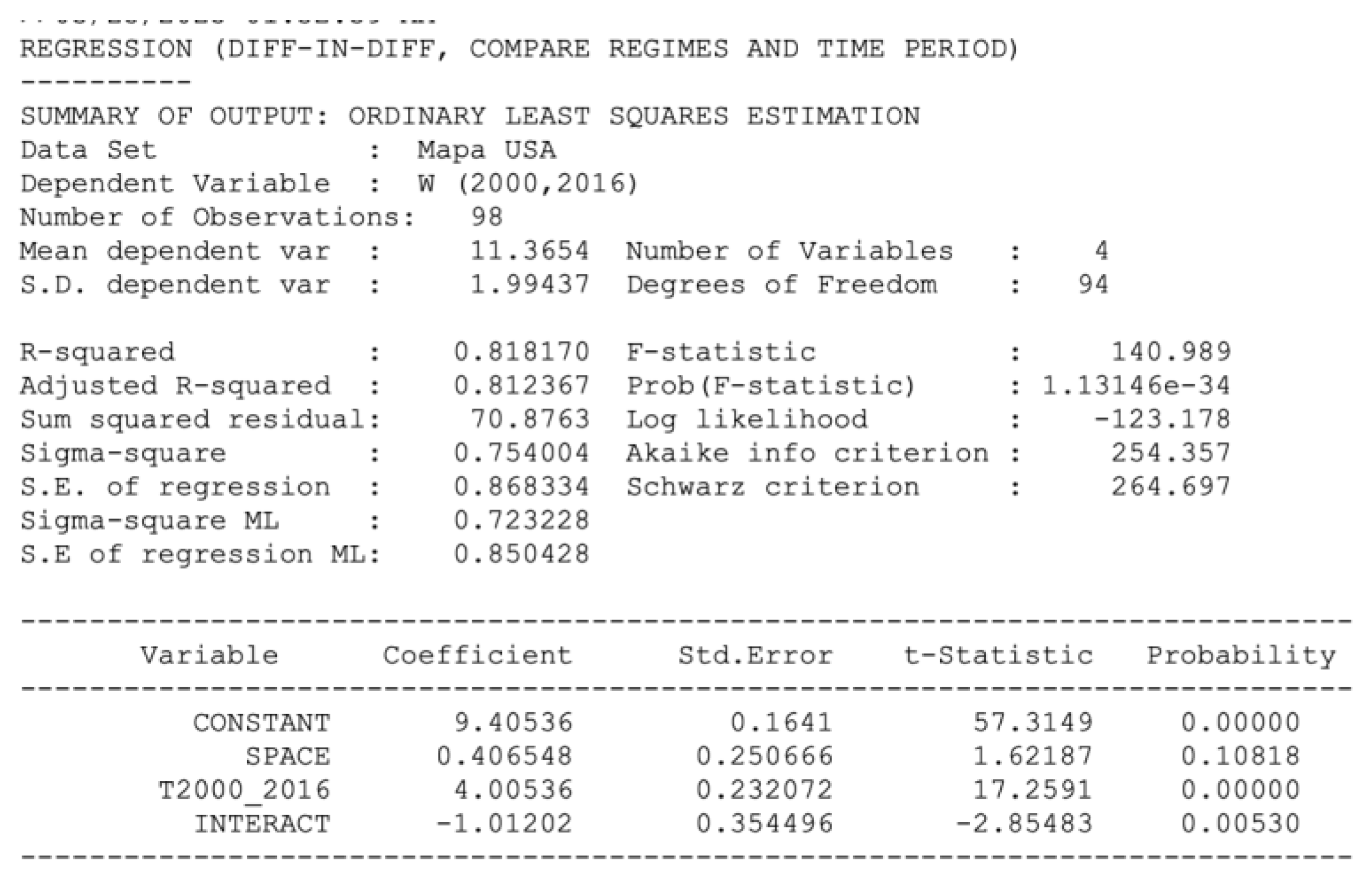
- Difference-in-Difference test
4. Conclusions
Appendix A. Mapping Smoothed Rates (See Anselin 2023)
- 1)
- Variance instability of rates
- 2)
- Borrowing strength
- 3)
- Bayes Law
| 1 | In descriptive statistics, the range of a data set () is determined by subtracting the smallest value (sample minimum, ) from the largest value (sample maximum, ) in the set: . The range is given in the same units as the data and serves as a measure of statistical dispersion, like the variance and standard deviation. |
| 2 | The mean of a variable (), often referred to as the arithmetic average, is calculated by dividing the sum of all values of this variable by the sample size: . |
| 3 | In statistics, the normal distribution, also known as Gaussian distribution, represents a type of continuous probability distribution. The general form of its probability density function is . Normal distributions are commonly used to represent real-valued random variables with unknown distributions due to the Central Limit Theorem, which asserts that the average of multiple samples from a random variable with a defined mean and variance will approximate a normal distribution as the sample size increases, assuming certain conditions are met. The normal distribution is symmetric around the mean value, which is also equal to the mode and median. It is unimodal and the total area between the curve and the x-axis, is equal to one. Approximately 68% of values from a normal distribution fall within one standard deviation (σ) of the mean, about 95% within two standard deviations, and roughly 99.7% within three standard deviations. This phenomenon is referred to as the 68-95-99.7 (empirical) rule, or the three-sigma rule. The most fundamental form of a normal distribution is the standard normal distribution, which occurs when the mean is 0 and the variance is 1. |
| 4 | In statistics, quartiles are a specific type of quantile that divides the data into four equal parts once the data is sorted from lowest to highest. There are three quartiles that segment the data into four groups. The first quartile (Q1), or lower quartile, marks the 25th percentile, meaning 25% of the data falls below this point. The second quartile (Q2) is the median, indicating that half of the data lies below this value. The third quartile (Q3), or upper quartile, is the 75th percentile, where 75% of the data is below this point. |
| 5 | In statistics, variance () measures the spread of a random variable's values () around its mean, calculated as the expected value of the squared differences from the mean: . Standard deviation (), derived as the square root of variance, quantifies the amount of variation or dispersion in a set of data values. Variance serves as the second central moment of a distribution and represents the covariance of the variable with itself. |
| 6 |
Pearson’s correlation coefficient is a statistical metric that quantifies the degree to which two variables are linearly associated, indicating their tendency to move together at a consistent rate. It is defined as the quotient between the covariance of these variables and the product of their respective standard deviation: . It is frequently used to depict straightforward relationships without implying causality. The correlation coefficient, varying from -1 to 1, indicates the strength and direction of a linear relationship between two variables. An absolute value of 1 signifies a perfect linear equation where all observations lie precisely on a line. If the coefficient is +1, increases with ; if it is -1, decreases as increases. A correlation of 0 means there is no linear association between the variables. Correlation analysis has limitations. It does not consider the influence of other variables beyond the two examined, nor does it establish causation, and it is ineffective at describing relationships that are curvilinear. |
| 7 | Simple linear regression in statistics is a model that uses one explanatory variable to predict the dependent variable through a linear function. It deals with two-dimensional sample points, mapping one independent variable to one dependent variable (typically represented as x and y in a Cartesian coordinate system). |
| 8 | OLS is a method used in simple linear regression to determine the best-fit line by minimizing the sum of the squares of the differences between observed and predicted values of the dependent variable, that is the sum of squares of the regression error term: . This optimization technique seeks to find the line that most closely aligns with the data points, providing unbiased estimates for the intercept () and slope () parameters in the model. The slope can also be expressed as: . In the case of a simple linear regression with standardised variables, the standard deviation of both variables is one and, therefore, the slope will coincide with the correlation coefficient. In this case, since , the intercept is equal to the mean value of the dependent variable. |
| 9 | If the numerator of the ratio variable represents the number of successes or occurrences and the denominator represents the total opportunities for the event to happen, then their division gives a direct estimate of the likelihood or probability of the event per unit of the population. According to the Law of Large Numbers, the average of the results obtained from a large number of trials or sample size (e.g. districts) should be close to the expected value and will tend to become closer as more trials are performed: . On its side, the Central Limit Theorem supports the use of ratio variables as unbiased estimators by stating that when an adequate sample size is used, the distribution of the sample ratios will approximate a normal distribution centered around the true probability: . |
| 10 | The Poisson-Gamma or Gamma-Poisson distribution is a statistical distribution for overdispersed count data. It is a versatile two-parameter family of continuous probability distributions. The exponential distribution and chi-squared distribution are special cases of the gamma distribution. There are two equivalent parameterizations in common use: 1) With a shape parameter and a scale parameter and 2) with a shape parameter α and a rate parameter . Bayesian statisticians prefer the parameterization, while the parameterization with and appears to be more common in econometrics and other applied fields (Wikipedia 2025a). |
| 11 | A Gamma distribution, characterized by shape parameter α and scale parameter , has a mean of the product of its shape and scale parameters: and the variance is . |
| 12 | From here, is the equivalent of . |
| 13 | A t-test is a statistical method utilized to compare the means of two groups. It is employed in hypothesis testing to assess whether a specific treatment influences the target population, or to determine if there is a significant difference between two groups. , where and are the means of the two groups being compared, is the pooled standard error of the two groups, (for the pooled standard deviation and the total sample), and , denote the number of observations in each group. A higher t-value indicates that the difference between the group means exceeds the pooled standard error, suggesting more difference between the groups. (Scribbr 2025). |
| 14 | The F-statistic fundamentally evaluates whether the inclusion of an explanatory variable yields a statistically significant improvement in model fit relative to a model containing only the intercept, or the overall mean. The computation of this statistic involves the regression sum of squared residuals () and the total sum of squared deviations of the dependent variable from its mean (). The resulting F-statistic in the context of the simple regression, with a constant and a binary (dummy) variable, is given by: , where , which implies that the F-statistic is evaluated with degrees of freedom equal to 1 and . See Anselin and Rey (2014), pp. 98-99. |
| 15 | In a Bayesian framework, the likelihood is defined as the probability of observing the data given a specific value (or distribution) of the parameters. Conversely, classical statistics typically consider the probability of the parameters based on the observed data. |
| 16 | Note that in this case, represents a set of parameters and not the scale parameter of the Gamma distribution. |
References
- Angrist, J, Pischke, J-S (2015) Mastering Metrics, the Path from Cause to Effect. Princeton, New Jersey: Princeton University Press.
- Anselin, L. (2023) An Introduction to Spatial Data Science with GeoDa. Volume 1: Exploring Spatial Data. https://lanselin.github.io/introbook_vol1.
- Anselin, L, Rey, S.J. (2014) Modern Spatial Econometrics in Practice, a Guide to Geoda, Geodaspace and Pysal. Chicago, IL: GeoDa Press.
- Anselin, L, Lozano-Gracia, N, Koschinky J (2006) Rate Transformations and Smoothing. Technical Report. Urbana, IL: Spatial Analysis Laboratory, Department of Geography, University of Illinois.
- Bivand, R.S. (2010) Exploratory Spatial Data Analysis. In Fischer, M.M., Getis, A., Eds.; Handbook of Applied Spatial Analysis: Software Tools, Methods and Applications; Springer: Berlin, Heidelberg; pp. 219–254 ISBN 978-3-642-03647-7.
- Brewer, C.A. (1997) Spectral Schemes: Controversial Color Use on Maps. Cartography and Geographic Information Systems 49: 280–94.
- Chasco, C., Vallone, A. (2023). Introduction to Cross-Section Spatial Econometric Models with Applications in R. Preprints. [CrossRef]
- Inselberg, A. (1985) The Plane with Parallel Coordinates. Visual Computer 1: 69–91.
- James, W, Stein, C (1961) Estimation with Quadratic Loss. Proceedings of the Fourth Berkeley Symposium on Mathematical Statistics and Probability 1: 361–79.
- Jenks, G. F. (1977) Optimal Data Classification for Choropleth Maps. Occasional. Paper no. 2. Lawrence, KS: Department of Geography, University of Kansas.
- Lefebvre, H. (1992) The Production of Space; Wiley-Blackwell: Oxford (UK) & Cambridge (USA), 1992; ISBN 978-0-631-18177-4.
- Loader, C. (2004) Smoothing: Local Regression Techniques. In Gentle, J.E., Härdle, W., Mori, Y. (eds.) Handbook of Computational Statistics: Concepts and Methods, Berlin: Springer-Verlag, pp. 539–63.
- Scribbr (2025) An Introduction to t Tests | Definitions, Formula and Examples. Accessed in March 2025. https://tinyurl.com/mud65hf9.
- Tobler, W.R. (1970) A Computer Movie Simulating Urban Growth in the Detroit Region. Economic Geography, 46, 234–240, . [CrossRef]
- Tukey, J. (1977) Exploratory Data Analysis. Reading, MA: Addison Wesley.
- Wikipedia (2025a) Gamma distribution. Accessed in March 2025. https://tinyurl.com/48yy28bc.
- Wikipedia (2025b) Bar chart. Accessed in March 2025. https://tinyurl.com/2dtws4zn.
- Wikipedia (2025c) Bayesian inference. Accessed in March 2025. https://tinyurl.com/mrxrvyxr.

| Dependent variable | ESDA tool | Econometric model |
|---|---|---|
| Continuous | Histogram Box plot Quantile map Natural break map Box map |
Spatial linear regression models Spatial Expansion models Geographically Weighted Regres. Trend surface models Spatial ridge and lasso models Spatial Partial Least Squares |
| Discrete | Bar chart Unique values |
Spatial count data models Binary Spatial models Spatial logit models Spatial probit models |
| Rates | Raw rate map Excess risk map Empirical Bayes smoothed rate map |
Spatial beta regression models Spatial fractional response mod. Spatial logit, probit, tobit mod. |
| Space-Time | Box plot over time Scatter plot with time lagged vars. Thematic map over time Difference in means Difference-in-difference |
Spatiotemporal models Spatial panel data models Difference-in-difference models |
Disclaimer/Publisher’s Note: The statements, opinions and data contained in all publications are solely those of the individual author(s) and contributor(s) and not of MDPI and/or the editor(s). MDPI and/or the editor(s) disclaim responsibility for any injury to people or property resulting from any ideas, methods, instructions or products referred to in the content. |
© 2025 by the author. Licensee MDPI, Basel, Switzerland. This article is an open access article distributed under the terms and conditions of the Creative Commons Attribution (CC BY) license (https://creativecommons.org/licenses/by/4.0/).


