
Submitted:
24 March 2025
Posted:
27 March 2025
You are already at the latest version
Abstract
Cement paste is a hydraulic binding agent made of water and cement. It gives the concrete its solid material matrix when hardened. The hardening of the cement paste relies on the exothermic chemical process referred to as hydration. The progress of the hydration and the associated development of the mechanical material properties depend primarily on the materials' composition and the hydration temperature. These circumstances were taken into account in the design of this experimental study by deliberately varying the water-to-cement mass ratio and the specimen size. A test series on cement paste made of ordinary Portland cement and tap water was conducted using the ultrasonic pulse transmission method with combined compression and shear wave measurement. All measurement data and metadata were finally compiled into datasets in the open-source, binary file format of GNU Octave. These datasets can serve as a database for the development of mechanical models or for feature extraction in the context of machine learning.
Keywords:
non-destructive
; ultrasound
; pulse transmission
; cement paste
1. Background & Summary
Concrete is currently, by far, the most commonly used material for manufacturing building structures. This building material consists of gravel, sand and cement paste. The cement paste is the adhesive that holds the gravel and sand together. It is made of cement and water and undergoes an exothermic chemical reaction called hydration. The reaction product, the cement stone, gives the concrete its solid material matrix. In technical applications, the mechanical properties of concrete are of utmost importance. The development of the mechanical properties of the cement paste governs the development of these properties.
While elastoplastic material models have long been established for hardened concrete, they are still under development for the early stage of the hydration process. Designing well-suited material models depends heavily on mechanical test methods, which provide the necessary data. Since the classic test methods used for solids cannot be applied to soft, viscoelastic test specimens such as cement paste, ultrasonic pulse reflection and ultrasonic pulse transmission methods have become established testing methods in this field.
In the relevant literature, neither conclusive mechanical material models nor measurement data are currently available for cement paste in the early hydration stage. The experimental study described here was carried out to remedy this situation. It provides the required measurement data and thus paves the way for designing material models for cement paste in the early hydration stage.
A considerable part of the chemical reaction occurs in the early stages of cement paste hydration. The reaction process depends mainly on the mixing ratio of cement and water and the thermal conditions during the chemical reaction. Therefore, this study focuses on the time and temperature-dependent development of the material properties within the first 24 hours after mixing cement and water. The ultrasonic pulse transmission method using piezoelectric contact probes was chosen because it is well suited for fully automated and quasi-continuous sound wave measurements of pasty materials.
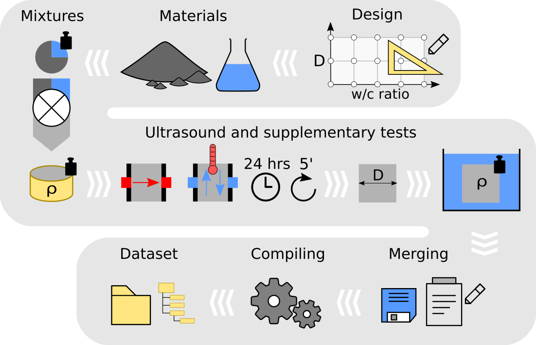
Besides the ultrasound tests, auxiliary tests were conducted (e.g. ultrasonic measuring distance and specimen density). These provide further information on the properties of the cement paste specimen before, during and after the ultrasound tests. The raw measurement data and metadata from these tests were combined with the ultrasound signal data to form a data set made of text files. The raw data were then compiled into a single binary file. The content of the binary data sets is hierarchically structured, machine-readable and available in the open-source file format of GNU Octave. In Figure 1, p.2, please find a summary of all procedural components of this experimental study.
In addition to the experimental study on cement pastes, further reference test series were created. Water, air and an aluminium cylinder were used as reference materials. Since these materials have known material properties, the test results are suitable to validate whether the ultrasound test results reproducibly reflect the physical laws of sound propagation. Therefore, the data of those reference test series are used in this work to verify the technical validity of the measurement results.
All data records referenced here are licensed under the Creative Commons Attribution 4.0 International[1] license and are available for download from the repository[2] of Graz University of Technology. That permits researchers who do not have access to the necessary experimental equipment, materials or laboratory facilities to benefit from this experimental data.
The data records provided are suitable for developing well-suited signal analysis methods and material models, feature extraction and creating training sets for machine learning. In addition, the data can serve as a reference for alternative test setups, materials and analysis methods.
In the past, a subset of the datasets from this study were the basis of the analysis results presented in the form of two conference papers by the author of this study. The first conference paper (see Harden[3], 2023) proposes a method to detect drift signals observed in the ultrasound signal data. The method is based on weighted stochastic properties measured in overlapping signal partitions. The second conference paper (see Harden[4], 2023) concerns signal disturbance characterization and temporal localization. The investigated disturbance is the induction current caused by the electromagnetic field emerging from the high-voltage pulse excitation of the piezoelectric activator. Besides the signal’s visual inspection to characterize the disturbance, a matched-filter technique was used for the temporal localization.
2. Methods
This section first explains the task, the experimental design and the experimental setup of this study. Then, the materials and the mixtures produced from them are described. Furthermore, the testing devices, the testing device settings, the individual steps of the experiments and the acquisition of the experimental data are comprehensibly detailed. Finally, the methodology of the dataset compilation and the technical validation of the experimental data is presented.
2.1. Study Design
The task underlying this experimental study is to create a database. This should serve as a basis for describing the mechanical properties of cement pastes in the early stages of hydration based on the ultrasonic pulse transmission method. In order to be able to use the results for technical applications, this study is based on the boundary conditions summarized below.
In the early phase of hydration, a substantial part of the exothermic chemical reaction between water and cement occurs. That means that the mechanical properties also change most strongly and most quickly in this phase. As with any chemical reaction, the reaction rate, the reaction temperature and the properties of the reaction products are closely related to the underlying reactive materials and the thermal conditions during the reaction. This time-dependent evolution of the physical properties of cement paste is discussed by Maruyama[5] and Igarashi (2014).
In addition to the evolution of the chemical reaction, the compressive strength after 28 days is of crucial importance for the technical use of cement paste in cement mortars and concrete. The strength of hardened concrete is closely related to the water-to-cement mass ratio ( ratio) of the cement paste and the strength class of the cement. In construction technology, mainly standard concretes with cylinder compressive strengths between 20 and 40 MegaPascals are used. These strengths correspond to the compressive strength classes C20/25, C25/30, C30/37, C35/45, C40/50 defined in Eurocode 2[6]. The reciprocal relationship between the compressive strength and the ratio was first presented by Abrams[7] (1918). Nagaraj[8] and Banu (1996) give a generalisation of this relationship. The influence of the cement strength in the context of that generalised relationship is discussed by Kargari[9] et al. (2019).
For the technically efficient use of cement, it is important to ensure that enough water is added to the mixture to allow the cement to react completely. The optimal amount of water depends mainly on the chemical composition of the cement, the specific weight and the specific surface area of the cement grains. In an experimental study by Wong[10] and Buenfeld (2009), the optimal water-cement ratio () for ordinary Portland cement (OPC) was determined to be 0.23. However, for mixtures without superplasticisers a notable higher ratio in the range of 0.4 and above is used to ensure the workability of cement mortars and concrete. The amount of excess-water depends on a whole range of factors (e.g. grain size distribution of the aggregate, cement content of the mixture). The dependency between the ratio and the workability of mortars is discussed in a paper by Haach[11] et al. (2011). However, the present study focuses on frequently occurring technical applications. Therefore, the study’s lower limit for the ratio is set to 0.4.
Apart from strength and workability, attention must also be paid to the stability of the mixture. A stable mixture of water and cement should be easy to homogenize and not tend to bleed. Bleeding means that some of the water settles again after mixing. This behaviour is often observed at ratios greater than 0.6. This issue is dealt with in detail in a paper by Ji[12] et al. (2019). Based on these findings, the study’s upper limit for the ratio is set to 0.6.
A geometric boundary condition is given by the ultrasound test apparatus. Before performing the ultrasound tests, the cement paste is loaded into moulds. These consist of two acrylic glass panels with integrated ultrasound contact probes. The vertical cross-sectional area of the interior of the mould, parallel to the acrylic glass panels, is constant. Therefore, the specimen’s volume is determined by the horizontal distance between the two opposite panels. However, this distance can be varied with appropriate spacers and is similar to the distance travelled by the sound wave (ultrasonic measuring distance D).
Study parameters:
Based on the properties of the chemical reaction of cement paste, the range of technical applications and the boundary conditions given by the test device, the two essential parameters of this study were identified.
- Mixing ratio of water and cement : The mixing ratio has an important influence on the reaction rate, the reaction temperature and the physical properties of the reaction products.
- Ultrasonic measuring distance : The ultrasonic measuring distance is a measure of the specimen’s volume. Furthermore, the ratio of surface area to volume of the specimen is closely related to the thermal energy balance of the chemical reaction due to the heat flux through the moulds perimeter.
In order to cover the broadest possible spectrum of material behaviour, these two parameters were varied in this study. The parameter variation was deliberately limited with respect to the findings and hints in the aforementioned literature.
Parameter variation:
The values listed below were selected for the previously identified test parameters and their limit values. They represent the basis for the ultrasound tests and, thus, the core of this study.
- Ultrasonic measuring distances mm
- Water-cement ratios
- Ultrasound test duration of 24 hours
- Ultrasound signal recordings at five-minute intervals
- Six test runs for each parameter pair (D, )
The test duration of 24 hours allows to cover a considerable part of the hardening process of the cement paste. The measurement interval of five minutes is related to the reaction rate already known from many technical applications and the literature (e.g. Ippei[5] and Maruyama, 2014). The six test runs were performed to assess the reproducibility of the tests and to receive hints concerning the stochastic properties of the measuring results.
Reference test series:
In addition to the test series for cement paste (Test series 1), further reference test series (Test series 5, Test series 6, Test series 7) were conducted using air, water and an aluminium cylinder as testing materials. These test series serve to investigate the applicability of the ultrasonic test device to different materials and to validate the stability with regard to the reproducibility of the measurement results. Using that reference data for device calibration purposes or accuracy assessments is not intended. This fact is also reflected in the partly roughly estimated ultrasonic measuring distances (see also subsection ‘Testing Procedures’, p. 19 and section ‘Technical Validation’ p. 35). The reference test series’ data records are also referenced and described in this work and serve to validate the ultrasound measurements at a technical level. The primary goals of this validation are to assess whether the ultrasound signal recordings reproducibly reflect the fundamental physical principles of sound propagation.
2.2. Experimental Setup
The laboratory tests carried out during this study consist primarily of ultrasonic pulse transmission tests. This testing method is the state-of-the-art technique (e.g. Lim[13] et al., 2018) for testing cement paste, cement mortar and concrete in the early stages of hydration. The test device used for the ultrasound tests is the FreshConDUO device presented by Ruck et al.[14] (2021). The following explanations motivate the underlying measuring principle and its technical implementation.
Measuring principle:
The measuring principle of the ultrasonic pulse transmission method using piezoelectric elements consists of the fundamental processes (1) excitation, (2) transmission and (3) observation.
- Excitation: The particles of a medium are excited to vibrate by a sound source. In the testing method used here, a piezoelectric contact probe (activator) is excited by a single pulse from a high-voltage pulse generator. The piezoelectric element in the contact probe deforms due to the applied voltage and thus excites the adjacent test body to vibrate. This behaviour is referred to as the piezoelectric effect (e.g. Ruediger[15], 2021).
- Transmission: The sound wave spreads out in the medium. The propagation speed of the sound wave (speed of sound) and the wave mode (longitudinal or transverse wave) depend on the mechanical properties of the medium. The sound wave is transmitted through the test specimen, which is positioned between the contact probes.
- Observation: The observer (a measuring instrument), who perceives the incoming sound wave, is located at a defined distance from the sound source. In the testing method used here, the measuring device is a piezoelectric contact probe (sensor). The piezoelectric element in the contact probe is deformed by the sound pressure and generates an electrical voltage (inverse piezoelectric effect). The analogue-digital converter of a data acquisition unit connected to the probe converts the voltage into a digital signal.
Ultrasonic pulse transmission tests:
The ultrasound testing device used for this study is the FreshConDUO[14] device. This testing device is designed for fully automated ultrasonic tests on mortar and concrete and fully reflects the measuring principle described above. Special concern was given to the fact that sound waves in solid and viscoelastic materials propagate not only as longitudinal waves (as in air and water) but also as transverse waves (e.g. Yoshida[16], 2024).
For this reason, the FreshConDUO device has two independent excitation and measurement systems. One for the longitudinal wave measurement – these are also referred to as compression waves or primary waves – and a second for the transverse wave measurement – these are also referred to as shear waves or secondary waves.
The experimental apparatus also provides a temperature measuring system to record the test specimen’s temperature. That measuring system is based on the thermoelectric effect of a coupled pair of conductors made of different metals also referred to as thermocouples (e.g. Roeser[17], 1940).
The individual components of the experimental apparatus are detailed in the following list. Please, find the corresponding schematic illustration in Figure 2, p.5.
- Measuring computer on which the test control and data recording software FreshCon 4.01[18] is installed (CTL).
- Pulse trigger unit to synchronize pulse excitation and signal recording (PTU).
- High-voltage pulse generator for stimulating the activators (HVP).
- Moulds with built-in activators and sensors (M1, M2). See Figure 3, p.6.
- Oscilloscope to record the ultrasound signal data (OSZ).
- Data acquisition unit to record the specimen temperature (DAQ).
- Thermocouple conductor wires (T1, T2, T3, T4). See Figure 4, p.7.
- Signal cables (two-wire BNC) connecting PTU, OSZ and HVP.
- Signal cables (two-wire BNC) connecting HVP with M1 and M2 (pulse).
- Signal cables (two-wire BNC) connecting OSZ with M1 and M2 (signal).
- USB cables connecting PTU, OSZ and DAQ with CTL (power supply, data transfer).
Auxiliary tests:
In addition to the ultrasound tests, auxiliary tests were carried out to determine the environmental conditions and the properties of the specimens before and after the ultrasonic tests. The test equipment used for this purpose as well as for the ultrasound measurements are described in subsection ‘Testing Devices’, p. 7.
2.3. Testing Devices
The testing devices listed in Table 1, p.8 include the devices used for all laboratory tests during this study. Nevertheless, this list is limited to those devices that may influence the measurement results of the ultrasound and the auxiliary tests. Nevertheless, the measuring device specifications are of utmost importance. These were taken from the manufacturer’s data sheets and are summarized in Table 2, p.9. Furthermore, a subset of the testing devices was assigned to device groups related to distinct testing procedures. The device group definitions, please find in Table 3, p.9. Finally, the ultrasound testing device settings are described.
Testing device settings:
The testing device settings listed below are limited to those related to the ultrasound tests and thus affect the ultrasound measuring results. The software settings are also displayed here since the test control and recording software FreshCon 4.01 is an integral part of the ultrasound testing device FreshConDUO. No particular settings had to be made for all other testing devices. All device and software settings are also available from the individual binary data set files described in section ‘Data Structure – Compiled Binary Datasets’ p. 33.
-
Oscilloscope (Table 1, p.8, d10)
- –
- Sampling rate: 10 MHz
- –
- Ensemble averaging: five measurements per sample
-
High-voltage pulse generator (Table 1, p.8, d12)
- –
- Pulse voltage: 800 V in Test series 1; 400, 600 and 800 V in Test series 5, Test series 6 and Test series 7.
- –
- Pulse width: 2.5 s
-
Test control and data recording software FreshCon 4.01
- –
- Record primary channel (compression wave signal)
- –
- Record secondary channel (shear wave signal)
- –
- Record specimen temperature (four channels)
- –
- Time delay between measurements: 5 minutes
- –
- Number of tests (equal to a test duration of 24 hours)
- –
- Number of samples recorded before pulse excitation (prefix section length), or samples
2.4. Materials
In Test series 1, cement pastes were investigated in the early stages of hydration. First, the materials and mixtures used for the cement paste tests are specified. Second, information on the reference materials used in Test series 5, Test series 6, and Test series 7 is provided. Finally, auxiliary materials supporting the testing processes are described.
Mixture components:
The cement pastes examined were made exclusively from ordinary Portland cement and tap water. The cement used in Test series 1 comes from two different batches. For all mixtures produced up to March 28, 2021, the cement comes from batch 34A. For all tests conducted later, cement from from batch 35A was used. The cement was stored on the same laboratory premises where the ultrasound tests were carried out. The tap water comes from the laboratory’s water supply system and is fed from a container where the water is kept at room temperature. Therefore, the temperature of the materials was not explicitly recorded. However, the environment temperature measurements provide a helpful indication of the material’s temperature. A brief description of the mixture components and the materials used for the reference tests, please find in Table 4, p.10.
Mixture recipes:
The mixture recipes for the cement pastes are designed to cover the typical industrial applications. Five mixture compositions with the following water-cement ratios were chosen: . The mass calculations of the mixtures are related to the volume of two moulds of the ultrasound testing device. Since the mould’s volume depends on the designated ultrasonic measuring distances mm, the mixture compositions shown in Table 5, p.11 are broken down according to the water-cement ratio and the ultrasonic measuring distance D.
Reference materials:
In addition to Test series 1 on cement pastes, several other ultrasound tests were carried out using materials with known material parameters (air, water, aluminium). These serve as a reference for the cement paste tests and allow for assessing the reproducibility of the ultrasound tests. The reference materials are listed according to the respective test series below.
Auxiliary materials:
Additional materials (see Table 6, p.12, m6 to m10) were used to prepare the moulds and specimen for the ultrasound tests on cement pastes. The application of these materials is explained in the sampling procedure in subsection ‘Testing Procedures’, p. 19. Apart from that, this list also covers the materials the components of the moulds of the ultrasonic testing device are made of (see Table 6, p.12, m11 to m14).

Table 6.
Table of auxiliary materials. Legend: MID …unique material identifier; PMMA …polymethyl methacrylate; EPDM …ethylene propylene diene monomer rubber; POM …polyoxymethylene.
Table 6.
Table of auxiliary materials. Legend: MID …unique material identifier; PMMA …polymethyl methacrylate; EPDM …ethylene propylene diene monomer rubber; POM …polyoxymethylene.
| MID | Description | Material | Vendor |
|---|---|---|---|
| m6 | Release agent | Corn germ oil | Mazola |
| m7 | Adhesive tape | Polyimide film tape 5413width = 50.8 mmthickness = 0.069 mm | 3M |
| m8 | Cling film | Polyethylene | N/A |
| m9 | Air balloon | Latex | N/A |
| m10 | Vaseline grease | Paraffin | N/A |
| m11 | Acrylic glass panel | PMMAthickness = 12 mm | N/A |
| m12 | Rubber foam spacer | Cell-caoutchouc, EPDMthickness = 25 mm | N/A |
| m13 | XPS board spacer | Extruded Polystyreneembossed surfacethickness = 20 mm | N/A |
| m14 | Sensor cover | Disk, POM | N/A |
2.5. Environmental Conditions
All laboratory tests were carried out in two air-conditioned rooms (Graz University of Technology, Campus Inffeldgasse, Construction Technology Center). Since these rooms are also used for accredited testing, the room temperature and relative humidity are kept within the limits specified below.
- Ambient temperature C
- Relative humidity %
2.6. Testing Procedures
This section describes the testing procedures of all laboratory tests conducted during this study. Since the laboratory test results of a test run are summarized in the individual datasets of a test series, the relationship between the test series and the laboratory test is established first. Then, the individual laboratory test procedures are explained in detail. The central element of each test run is the ultrasonic pulse transmission test. All other tests provide additional information on the tested specimen and the ambient conditions before, during and after the ultrasound test. Please find a schematic representation of the test sequence of a test run on cement paste in Figure 5, p.19.
The following laboratory tests were carried out for Test series 1. The associated tests and testing equipment, please find in Table 7, p.13, Table 8, p.14, Table 9, p.15, Table 10, p.16 and Table 11, p.17.
- Environment temperature (ENV)
- Mixture composing procedure (MIX)
- Fresh paste density (FPD)
- Sampling procedure (SMP)
- Specimen temperature (TEM)
- Ultrasonic pulse transmission tests (UTT)
- Ultrasonic measuring distance (UMD)
- Solid specimen density (SSD)
- Specimen archiving (ARC)
Due to the nature of the testing material, a workflow different from the one shown above was chosen for the reference tests in Test series 5, Test series 6 and Test series 7. The differences are mainly related to the measurement of the specimen density, temperature, and specimen preparation. The associated tests and testing equipment, please find in Table 12, p.18.
-
Test series 5, reference tests on air
- Environment temperature and humidity (ENV2)
- –
- Sampling procedure (SMP2)
- –
- Ultrasonic pulse transmission tests (UTT)
- –
- Ultrasonic measuring distance (UMD2)
-
Test series 6, reference tests on water
- –
- Environment temperature and humidity (ENV2)
- –
- Sampling procedure (SMP3)
- –
- Ultrasonic pulse transmission tests (UTT)
- –
- Ultrasonic measuring distance (UMD2)
-
Test series 7, reference tests on aluminum cylinder
- –
- Environment temperature and humidity (ENV2)
- –
- Sampling procedure (SMP4)
- –
- Ultrasonic pulse transmission tests (UTT2)
- –
- Ultrasonic measuring distance (UMD3)
- –
- Solid specimen density (SSD2)
- –
- Specimen archiving (ARC2)
Environment temperature (ENV):
Before preparing the mixtures, the environment temperature was read from the room temperature logger and recorded in the laboratory protocol. The temperature logger is attached to the wall of the laboratory, approximately six meters apart from the ultrasonic testing device. At this point, it is to note that the measured values from the temperature logger and the environment temperature measurement using thermocouples (see testing procedure TEM) differ by approximately ∘C.
Environment temperature and humidity (ENV2):
For the reference tests in Test series 5, Test series 6 and Test series 7, deviating from the testing procedure ENV, the humidity was also recorded.
Mixture composing procedure (MIX):
The mixture composing procedure consists of weighing the mixture components and mixing. The masses of the mixture components were taken from Table 5, p.11 and weighed using a digital balance with an accuracy of g. The individual steps for producing the mixtures are listed below.
- Weigh mixture components (cement, water) according to the recipe
- Prepare mixer
- Pour cement in mixer bowl
- Add water to the cement and start counter-clock
- Mix for about 60 s
- 30 s scratching debris from the wall of the mixer bowl with a metal spoon
- Mix for about 90 s
Fresh paste density test (FPD):
The gravimetric determination of the density of the fresh cement paste was carried out directly after preparing the mixtures and before loading the moulds of the ultrasonic testing device. For this purpose, a graduated beaker and a digital balance were used. The weights were measured with an accuracy of g (see Table 2, p.9, d26). It should be noted that this test was not carried out in all test runs of Test series 1 and is therefore not available from all datasets. The individual steps of the testing procedure are listed below.
- Moist inner surface of graduated beaker using a wet towel
- Pour paste in beaker, fill beaker to approx. half height
- Shake beaker for approx. 10 sec (vertical movements)
- Pour paste in beaker, fill to top edge
- Shake beaker for approx. 10 sec (vertical movements)
- Assure that beaker is fully filled (plus 2-3 mm over the top edge)
- Scrape off excess material along the beaker edge with a trowel
- Tare balance
- Measure gross weight (beaker plus paste)
Sampling procedure (SMP):
The sampling of the test specimens consists of preparing the moulds of the ultrasonic testing device, loading the moulds with the cement paste, compacting the paste and placing the thermocouples for the specimen temperature measurement.
Since the ultrasonic contact probes are movably mounted in the moulds, a narrow annular gap ( mm width) exists between the probe and the mould’s acrylic glass panel. This gap was covered with adhesive polyimide film tape (see Table 6, p.12, m7) to prevent the cement paste from penetrating the gap. Before applying the tape, the bonding area was cleaned of dirt to ensure proper bonding. Then, the tape was applied vertically over the entire height of the acrylic glass panels, making sure to avoid air bubbles between the tape and the contact probe’s surface. Furthermore, the tape was replaced on visible damages in the surface areas of the ultrasonic contact probes.
Before assembling the moulds, the mould’s surface wetted by the cement paste was coated with a release agent made of ordinary corn germ oil (see Table 6, p.12, m6). The surface area of the ultrasonic contact probes was left out or, if necessary, cleaned with ethanol and a paper towel.
Two compaction processes were carried out while loading the moulds by vertically shaking them. Thereby, the mould was lifted on one side by about three to four centimetres and dropped again. The compaction prevents considerably large air bubbles from remaining in the space between the activator and the sensor (ultrasonic contact probes).
The different mould configurations, please find in Figure 3, p.6. The thermocouple placement is illustrated in Figure 4, p.7. The individual steps of the sampling procedure are listed below.
- Ensure that the gap between the ultrasound contact probes and the acrylic glass panels is covered properly with polyimide film tape.
- Apply release agent on surfaces of mould M1 and mould M2.
- If necessary, remove the release agent from surface areas of the contact probes.
- Assemble mould M1 and mould M2.
- Pour the cement paste into mould M1. Fill up to approximately half the height of the mould.
- Repeat step 5 for mould M2.
- Shake mould M1 for approx. 10 sec (vertical movements).
- Repeat step 7 for mould M2.
- Pour the paste into mould M1, fill up to approx. 2.5 cm below the top edge of the mould.
- Repeat step 9 for mould M2.
- Shake mould M1 for approx. 10 sec (vertical movements).
- Repeat step 11 for mould M2.
- Cover mould M1 with cover strips. See note below.
- Repeat step 13 for mould M2.
- Place thermocouples as explained in testing procedure TEM.
The sequential order of the cover strips is identical to the spacers depicted in the cross sections in Figure 3, p.6. In the Mould-70a configuration, cling film was used instead of cover strips to prevent the specimen from drying out during the test.
Sampling procedure 2 (SMP2):
No special procedures were used to prepare the test specimen for the ultrasound tests in Test series 5, reference tests on air. It is worth noting that the ultrasonic contact probes were not covered with polyimide film tape for this sampling procedure.
Sampling procedure 3 (SMP3):
Since the spacers shown in Figure 3, p.6 are not sufficiently waterproof, the water used for the ultrasound tests in Test series 6 was filled into air balloons (see Table 6, p.12, m9), which were subsequently placed between the activator and the sensor of both moulds. The same balloons were used for all ultrasonic measuring distances. For the distance mm, it was observed that the balloons hardly covered the contact probe’s surface. For this reason, water was added to the balloons, and the tests were repeated. These additional test turns are reflected in the turn number added to the end of the data set designations. This sampling procedure was always carried out without using spacers and covering the contact probes’ surfaces with polyimide film tape.
Sampling procedure 4 (SMP4):
In order to ensure a flat frictional connection between the aluminium cylinder and the contact probes, a skinny layer of grease (see Table 6, p.12, m10) was applied to the contact probe’s surfaces. The aluminium cylinder was then clamped directly between the contact probes, which were not covered with the polyimide film tape.
Specimen temperature (TEM):
The hydration temperature of the cement paste was measured using thermocouple probes. Before the measurement, three thermocouple wires T1, T2 and T3 were inserted from above into the still soft cement paste after loading the moulds as described in sampling procedure SMP. The hydration temperature was always measured in mould M2 (specimen II). In addition, the environment temperature was measured by placing the thermocouple wire T4 near mould M2. Please find the thermocouple wire’s proper placement in Figure 4, p.7. The individual preparation steps for the temperature measurement are listed below.
- Strip ends of thermocouples, approximately two centimetres long.
- Twist both strands together and bend them over, approximately one centimetre long.
- Repeat the first two steps for all thermocouple wires (T1, T2, T3, T4).
- Place thermocouple T1 in the centre of the specimen in mould M2.
- Place thermocouple T2 on the side panel of mould M2, next to the sensor, vertically centred to the specimens height.
- Place thermocouple T3 on the mid of the lateral surface of the spacer of mould M2, vertically centred to the specimens height.
- Place thermocouple T4 outside but right next to mould M2.
Steps 1 to 3 were always carried out before preparing the cement paste mixtures, and steps 4 to 7 were carried out after loading the cement paste into the moulds. Due to the division of the process steps, it was possible to keep the time between adding water to the cement and the beginning of the ultrasonic pulse transmission test as short as possible. The temperature recording was carried out automatically and simultaneously with the recording of the ultrasound signals. It has to be noted, that the specimen temperature test was not carried out in all test runs and is therefore not included in all datasets.
Ultrasonic pulse transmission test (UTT):
Immediately after loading the two moulds and placing the thermocouples, the ultrasonic pulse transmission test was performed. First, the test control and data recording software was started on the measuring computer and the test settings were configured as described in subsection ‘Testing Devices’, p. 7. Second, the automated test run was initiated manually on the control software. After the end of the test (24 hours), the hardened specimen were removed from both moulds and subjected to further tests. The individual steps for carrying out the ultrasonic pulse transmission tests are listed below.
- Check assembly of the testing device (moulds, cables, thermocouple wires).
- Assure that the cables between the pulse generator and actuators and the cables between the oscilloscope and sensors are not close to each other. See also note below.
- Start software on the measuring computer, configure the test settings and the time elapsed between adding water to the cement and the test initiation. See also sampling procedure SMP.
- Initiate the test.
- Wait for the test to end.
- Remove the specimen from the moulds by disassembling them.
- Clean the moulds.
Note to step 2: The BNC signal cables used are shielded. However, preceding tests using different cable placements showed that the inductive interference caused by the high-voltage pulse excitation was considerably smaller when the cables were not too close to each other.
Ultrasonic pulse transmission test 2 (UTT2):
Since only one aluminium cylinder was available, the ultrasound tests in Test series 7 were carried out as single-channel tests. First, all tests were carried out using the longitudinal characteristics activator and sensor in mould M1. Second, all tests were repeated using the transverse characteristics activator and sensor in mould M2. For both test runs, the procedure was the same as described in testing procedure UTT. Finally, the measurement data from both test runs were merged to construct the same data structure as returned by a two-channel test.
Ultrasonic measuring distance (UMD):
After removing the hardened cement paste specimen from the moulds, the ultrasonic measuring distance D was determined separately for each specimen. Due to the design of the moulds, the ultrasonic contact probes protrude approximately 0.5 mm from the surface of the acrylic glass panels and leave shallow depressions in the hardened test specimens. Therefore, it was impossible to determine the distance directly.
However, as aid, two steel washers were used to determine the distance. These were placed in the shallow depressions (hutches) on both sides of the specimen before measuring the distance. After measuring the total distance with the sliding calliper (specimen plus two washers), the thickness of the two washers was subtracted. The distance measurement was carried out using a digital sliding calliper and an accuracy of mm (see Table 2, p.9, d27). The individual steps for determining the ultrasonic measuring distance are listed below.
- Apply steel washer in hutches on both sides of the specimen.
- Measure total distance using a sliding calliper (thickness of specimen plus thickness of two washers).
- Subtract the thickness of two washers from the total distance.
Ultrasonic measuring distance 2 (UMD2):
For Test series 5 and Test series 6, the ultrasonic measuring distance D was determined by measuring the distance with a digital sliding calliper. Since the activator and the sensor are mounted movably in the moulds, an exact and stable measurement of the ultrasonic measuring distance was impossible. Instead, the inner distance between the acrylic glass panels of the moulds was determined with an accuracy of mm (see Table 2, p.9, d27).
Since air does not exert any pressure on the ultrasonic contact probes, they protrude up to 1.5 mm from the surface of the acrylic glass panels. For the reference tests with water, however, a similar situation arises as with cement paste. Due to the water pressure, the probes only protrude about 0.5 mm from the surface of the acrylic glass panels. For this reason, the ultrasonic measuring distance could only be roughly estimated on the basis of the distance between acrylic glass panels and the estimated protrusion.
Ultrasonic measuring distance 3 (UMD3):
For the tests in Test series 7, the ultrasonic measuring distance D was determined by the distance between the plane-parallel bottom and head surface of the cylinder. The distance measurement was carried out with a digital sliding calliper and an accuracy of mm (see Table 2, p.9, d27).
Solid specimen density (SSD):
The density of the solid test specimens was determined directly after measuring the ultrasonic measuring distance. The density test was done by immersion weighing according to the Archimedean principle. The surface of the test specimens was neither coated nor treated in any other way before immersion in the water basin.
In order to prevent the uncoated specimen from absorbing water, the immersion time was kept as short as possible at around 30 seconds. The water was observed to roll off the specimens after removing them from the water basin. That is most likely due to the release agent used to coat the moulds during the sampling procedure SMP.
The weight of the specimens was determined using digital scales with an accuracy of g (see Table 2, p.9, d25) or g (see Table 2, p.9, d24). The information, which scale was used is included in the datasets’ metadata. The individual steps of determining the solid specimen density are listed below.
- Remove loose parts from specimen edges.
- Tare balance.
- Weigh dry mass of the specimen.
- Lower the basket into the water container and attach it to the balance.
- Tare balance.
- Put the specimen on the basket, make sure that it is completely covered with water.
- Wait until air bubbles have disappeared from the specimen surface and it is hanging quietly in the water.
- Weigh floating mass of the specimen.
Solid specimen density 2 (SSD2):
In Test series 7 the density of the aluminium cylinder was determined gravimetrically. Due to the accurate geometric dimensions, the volume was calculated from the cylinder dimensions. These were measured with a digital sliding caliper and an accuracy of mm (see Table 2, p.9, d27). The weight of the cylinder was measured with a digital balance at an accuracy of g (see Table 2, p.9, d26).
Specimen archiving (ARC):
At the test’s end, the hardened cement paste specimens were archived. The archiving was carried out based on a guideline from Graz University of Technology for storing samples from scientific tests. That also offers the possibility of carrying out further tests on the test specimens in the future. The individual steps of the archiving procedure are listed below.
- Label the test specimen (specimen I and specimen II) with the assignment to the type of ultrasonic sensor types (`P’ or `S’). The `P’ denotes the primary channel 1 with compression wave sensors (longitudinal sensor characteristic). The `S’ denotes the secondary channel 2 with shear wave sensors (transverse sensor characteristic).
- Place both specimens of the ultrasonic test (`P’ and `S’) in one plastic bag and seal it with tape.
- Label the plastic bag with the sample number (data set designation), the name of the operator and the start date of the experiment.
- Stow plastic bags with specimens in indoor storage.
Specimen archiving 2 (ARC2):
The aluminium cylinder used for the tests in Test series 7 was packed in a plastic bag and labelled with the material name, weight and dimensions. The cylinder was also kept for later use.
2.7. Data Acquisition
The acquisition of data from the laboratory experiments was carried out either automatically or manually, depending on the type of experiment. A description of the two acquisition methods is given below. In Figure 6, p.26, please find a schematic representation of the data collection and processing workflow.
Automated data acquisition:
The signal data of the ultrasound tests (UTT, UTT2) and the specimen temperature (TEM) were recorded automatically by the test control and data recording software FreshCon 4.01. The software reads the digitized data from the data acquisition units (see Table 1, p.8, d10, d11) at specified measurement intervals over the entire test duration and stores them in files.
After the ultrasound test, the measurement data are available as human- and machine-readable text files. The respective folder and file structure of the recordings is explained in subsection ‘Data Structure – Raw Data Datasets’, p. 32.
One aspect of automated data acquisition using the FreshCon device[14] should be emphasised in particular. The USB oscilloscope (see Table 1, p.8, d10), which is part of the FreshConDUO device, has a built-in automatic amplitude pre-amplification with eleven voltage ranges (see Table 2, p.9, d10). Therefore, the signal responses of the compression and shear waves are scaled to some extent. The actual pre-amplification level of the oscilloscope is displayed on the screen but not recorded by the software and therefore not available. This aspect is also mentioned in the device’s user manual[18] on page 25. The pre-amplifications’ effect becomes particularly apparent in the graphical representations of the analysis results shown in section ‘Technical Validation’ p. 35.
Manual data acquisition:
The measurement data of all other laboratory tests (ENV, ENV2, FPD, UMD, UMD2, UMD3, SSD, SSD2) described in section ‘Testing Procedures’ p. 19 were recorded manually in handwritten laboratory protocols. The data were then transferred to a LibreOffice[32] Calc spreadsheet and exported as a comma-separated text file. These text files are the basis for the file projinfo.txt described in subsection ‘Data Structure – Raw Data Datasets’, p. 32. Subsequently, this file was assigned to the raw data of the individual datasets.
For the metadata (e.g. information on test equipment, materials, mixtures, procedures), metadata databases were created using the script collection Data set compiler 1.2[33] and the open-source binary file format of GNU Octave. These databases provide the metadata for the binary datasets compiled from the collected raw data. They are an integral part of the script collection Data set compiler 1.2 described in section ‘Code Availability’ p. 44.
It is worth mentioning that the projinfo.txt file contains only the record identification numbers from the metadata database instead of the complete metadata. Based on those identification numbers, metadata from the metadata databases is inserted into the binary datasets during compilation.
2.8. Computational Processing
The computational processing of the measurement data and the associated metadata refers exclusively to the fully automated compilation of the collected raw data into binary datasets. The measurement data were neither filtered nor modified in any other way. An illustration of this process, please find in Figure 6, p.26. The individual steps of the compilation process are listed below.
- Reading in the measurement data from the automated data acquisition (tst*.dat, tst.tem, measurements.txt, settings.txt).
- Reading in the measurement data from the manual data acquisition (projinfo.txt).
- Metadata structure assembly using the file `projinfo.txt’ and the metadata databases.
- Data structure assembly for the individual laboratory experiments from the measurement data.
- Dataset structure assembly using the already assembled data and metadata substructures.
- Saving the assembled data set structure in a data set file using the binary file format of GNU Octave.
The data processing steps are only roughly described here. To make the whole process comprehensible, the script collection Data set compiler 1.2 used for this task is also made available and described in section ‘Code Availability’ p. 44.
2.9. Analysis Methods for the Technical Validation
The analysis methods described here are used to justify the technical validity of the ultrasound measurement results. The validation aims to show that the recorded ultrasound signal data reproducibly reflects the underlying physical laws of sound propagation. The following explanations describe the selected materials (datasets), the analysis methods and the analysis procedure.
Materials (datasets):
To cover the broadest possible range of materials, a selection of data sets from the aforementioned reference tests with air, water and an aluminium cylinder are used. These materials cover all three aggregation states possible under normal ambient conditions. Since the physical properties of the reference materials are known from the literature, an independent prediction of the expected material behaviour concerning the given test conditions is possible. In addition to the material’s aggregate state, the ultrasonic measuring distance also plays an important role in the propagation of the sound waves. This circumstance is reflected by using signal data from ultrasound tests with various measuring distances. The following list retains the selection of the data sets subjected to the analysis.
-
Test series 5, reference tests on air[29]
- –
-
mm: ts5_d25_b16_v800.oct, ts5_d25_b24_v800.oct,ts5_d25_b33_v800.oct, ts5_d25_b50_v800.oct
- –
-
mm: ts5_d50_b16_v800.oct, ts5_d50_b24_v800.oct,ts5_d50_b33_v800.oct, ts5_d50_b50_v800.oct
- –
-
mm: ts5_d70_b16_v800.oct, ts5_d70_b24_v800.oct,ts5_d70_b33_v800.oct, ts5_d70_b50_v800.oct
-
Test series 6, reference tests on water[30]
- –
-
mm: ts6_d25_b16_v800.oct, ts6_d25_b24_v800.oct,ts6_d25_b33_v800.oct, ts6_d25_b50_v800.oct
- –
-
mm: ts6_d50_b16_v800.oct, ts6_d50_b24_v800.oct,ts6_d50_b33_v800.oct, ts6_d50_b50_v800.oct
- –
-
mm: ts6_d70_b16_v800.oct, ts6_d70_b24_v800.oct,ts6_d70_b33_v800.oct, ts6_d70_b50_v800.oct
-
Test series 7, reference tests on aluminum cylinder[31]
- –
-
mm: ts7_d50_b16_v800.oct, ts7_d50_b24_v800.oct,ts7_d50_b33_v800.oct, ts7_d50_b50_v800.oct
Each data set contains ten recordings of the signal responses of compression and shear waves. For air and water, however, only the signal responses of the compression wave are considered. For the aluminium cylinder, the signal responses of the shear waves are also considered since solid materials also transmit transverse waves.
Analysis methods:
To show that the ultrasound tests’ signal responses reflect the underlying physical laws of sound propagation, a prediction of the sound travel time is compared with compression and shear wave signal responses. In addition, the reproducibility of the tests is justified using the stochastic properties of signal sequences of repeated tests. The analysis methods used are briefly summarized in the following list.
- Estimating the sound travel time based on the ultrasound measurement distance and the literature data for the reference materials’ speed of sound. The ambient conditions (temperature, humidity), the measurement tolerances of the test equipment and procedural errors are taken into account in the estimation. Furthermore, it is assumed that the measured values and the associated tolerances are not correlated.
- Combining signal data from repeated tests to signal sequences. The ensemble average and the distribution of the deviations of the signal amplitudes from the ensemble average are determined from the signal sequences, as these reflect the average behaviour of the ultrasound test configuration more reliably. Minimum, maximum and quantiles characterize the distribution of the deviations.
- Visual comparison of the sound travel times of the first incoming wave and its reflections with the tolerance ranges of the predicted sound travel times.
- Visual comparison of the ensemble averages amplitudes of the first incoming wave and its reflections.
- Assessment of the reproducibility based on the characteristic properties of the deviations’ distribution.
Analysis procedure:
The subsequently described analysis procedure is derived from the task of technical validation and the chosen materials and methods. The detailed explanations do not aim to make the most accurate prediction possible but rather to consider all known boundary conditions.
oct2tex.param
-
Estimation of the ultrasonic measuring distance limits considering the measured distance D, procedural errors and the measuring device tolerances (see Table 2, p.9, d27). The source of the considerably high procedural errors are described in detail in the testing procedures UMD2 and UMD3 in subsection ‘Testing Procedures’, p. 19.
- –
- Air: mm
- –
- Water: mm
- –
- Aluminium cylinder: mm
- Estimation of temperature limits for the materials air and water considering the measured ambient temperature and the measuring device tolerances (see Table 2, p.9, d33). ∘C.
- Estimation of the humidity limits for air considering the measured ambient humidity U and the measuring device tolerances (see Table 2, p.9, d33). It is to be mentioned that the temperature-dependent measuring tolerance estimate () is based on the difference between the ambient temperature and the device calibration standard temperature (C). %.
-
Estimation of the aluminium cylinder’s density limits considering the cylinder dimensions, its weight and the measuring device tolerances (see Table 2, p.9, d26, d27).
- –
- Diameter: mm
- –
- Height: mm
- –
- Volume: cm3
- –
- Mass: g
- –
- Density: g/cm3
-
Estimation of the speed of sound limits based on literature values and the previously estimated limits for temperature and relative humidity . The speed of sound for air[34] and water[35] were interpolated linearly using the tabulated values from the literature. As the elastic properties of the aluminium cylinder were not explicitly measured, and no other more precise information on the actual material is available, the speed of sound was calculated (e.g. Garett[36], 2020) from the cylinder’s density and the elastic moduli taken from literature[37]. The tolerance limits for the Young’s modulus E and the shear modulus G refer to the tabulated values of the aluminium alloys 1100 and 2014.
- Air: m/s, where is a two-dimensional linear interpolation with the supports and realized by Octave’s built-in function interp1.
- –
- Water: m/s, where is a one-dimensional linear interpolation with the support realized by Octave’s built-in function interp2.
- –
-
Aluminium:
- *
- Poisson’s ratio for isotropic elastic materials.
- *
- Compression (longitudinal) wave in isotropic elastic materials.
- *
- Shear (transverse) wave in isotropic elastic materials.
- Estimation of the signal index at which the high-voltage pulse excitation apparently happened. A short period (trigger delay) passes between the zero point of the samples’ time signatures and the beginning of the inductive disturbance caused by the high-voltage pulse. The time period is too long to be explained by the propagation speed of the electromagnetic wave. The fact that several processor cycles are required to process the trigger event is a likely cause. This delay is estimated based on visual observations and existing analyses[4] with samples and added to the sound travel time estimates.
-
Estimation of the sound travel time tolerance ranges , , from the trigger delay limits , the ultrasonic measuring distance limits and the speed of sound limits for the first incoming sound wave and the first and second reflection of the sound wave.
- –
- Zero-time (trigger delay): s, sampling rate MHz (see testing device settings in subsection ‘Testing Devices’, p. 7)
- –
- Sound travel time of the first incoming wave: s
- –
- Sound travel time of the wave’ first reflection: s
- –
- Sound travel time of the wave’ second reflection: s
- Combining signals from different data sets of test repetitions into signal sequences. This results in a signal sequence including signals per distance and material.
-
Calculation of the ensemble average M and the distribution of the deviations R from the ensemble average. The distribution of R is thereby characterized by the minimum , the maximum , the lower quartile and the upper quartile . It is to be noted that the quartile estimates are realized using Octave’s built-in function quantile (method No.5).
- –
- Ensemble average
- –
- Deviation of individual signals
- Plotting the analysis results.
- Visual comparison of the estimated sound travel times with the ensemble average M.
- Visual inspection of the distribution R of the deviation from the ensemble average M.
The realization of the analysis procedure (GNU Octave code) is provided for comprehensibility and reproducibility reasons and referred to in section ‘Code Availability’ p. 44. The instructions for reproducing the analysis results are provided in section ‘Usage Notes’ p. 42. The results of the above–described analysis are presented in section ‘Technical Validation’ p. 35.
3. Data Records
This section is dedicated to describing the content and structure of all data records referenced in this work. These include the datasets from the experimental study on cement pastes and the datasets from the reference tests with air, water and the aluminium cylinder. The reference tests are subsequently used in section ‘Technical Validation’ p. 35 to assess the technical quality of the ultrasound measuring results. The following subsections explain the availability of the datasets, file naming conventions, file formats, content and the structure of the datasets included in the data records in detail.
3.1. Availability
All data records are made available as digital objects from the TU Graz Repository[2] – the officially registered file repository of Graz University of Technology. To ensure sustained usability, the they are licensed under the Creative Commons Attribution 4.0 International[1] license. The following list concludes the data records associated with this study.
3.2. Record Content
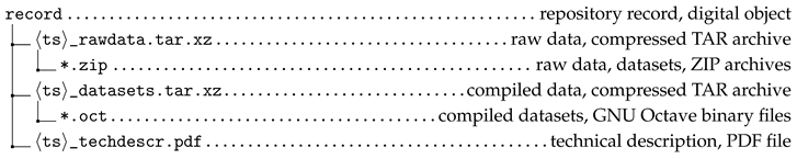
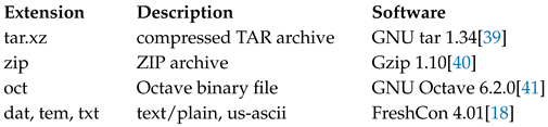
Each data record includes a compressed TAR archive containing the raw data of the laboratory experiments, a compressed TAR archive with the datasets compiled from them and a technical description in the form of a PDF file. The archive structure of each record is shown below. The 〈ts〉 prefix denotes the actual test series code, and the asterisk is a placeholder for the unique data set identifiers also referred here to as the data set designation.
Access to the record content:
Each of the aforementioned TAR archives contains the datasets of an entire test series. Therefore, the TAR archives must first be decompressed and unpacked. A description of the procedure and the required software is available in section ‘Usage Notes’ p. 42.
Dataset designation and filename conventions:
The datasets’ file names reflect the variation of each test series’ test parameters. The file names – without filename extension – represent the dataset designation. A meaningful file name makes searching for individual datasets easier, and its uniqueness enables clear referencing. Since the individual test series rely on different parameter variations, different conventions apply to the data set’s file names. The following listings provide an overview of the filename conventions of the respective test series. Additional examples explain how to read them.
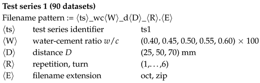
Example: ts1_wc055_d70_1.oct is a binary data set of test series 1. The water-cement ratio of the cement paste is 0.55, the ultrasonic measuring distance D is 70 mm, and the turn or repetition number is 1. The filename of the corresponding raw data archive is ts1_wc055_d70_1.zip.
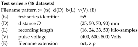
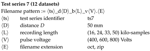
Example: ts5_d25_b50_v800.oct is a binary data set of test series 5. The ultrasonic measuring distance D is 25 mm, the recording length (block size) L is 50 kilo-samples, and the excitation pulse voltage V is 800 Volts. The file name of the corresponding raw data archive is ts5_d25_b50_v800.zip.
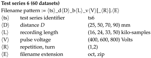
Please note that the repetition number 〈R〉 is available for the test runs of Test series 6 with mm only. This circumstance is explained in the sampling procedure SMP3 in section ‘Testing Procedures’ p. 19.
File formats:
For all files in the data records only open-source file formats are used. The file formats and the software used to create these files are listed below.
3.3. Data Structure – Raw Data Datasets
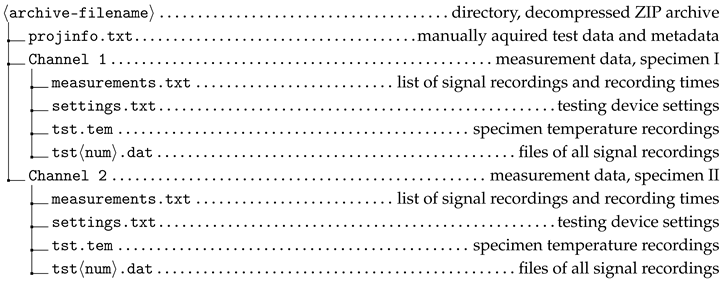
The raw data archives (*_rawdata.tar.xz) contain a set of ZIP archives (*.zip). These consist of the collected raw data from all experiments related to one test run. The raw data are human- and machine-readable text files whose contents have different structures. For all text files, comment lines always begin with two pond signs (##) which are silently ignored during machine interpretation. The tree view below shows the directory and file structure in the raw data ZIP archives.
File structure – projinfo.txt
The projinfo.txt file supplies all manually collected laboratory test results. In addition, this file contains the metadata about the test series and the tests. Each line of this file represents an independent entry with the following line format: [datatype] tag = value. The data type descriptor [datatype] in brackets can take one of the following values: (1) str for character arrays; (2) bool for Boolean values (true or false); (2) uint for unsigned integral numbers; sng for single precision floating point numbers (32 Bit); (3) dbl for double precision floating point numbers (64 Bit). Boolean values and character arrays (strings) are always surrounded by double-quotes (e.g. "string", "true").
File structure – measurements.txt
The measurements.txt file is a tab-separated text file. It contains a two-column list with file names (e.g. tst0001.dat) and the signal recording times (e.g. 01:26:30). The times refer to the time when the automated test execution was initiated (t = 0 s).
File structure – settings.txt
The settings.txt file is a tab-separated text file. It contains the software settings used to control the automated execution of the ultrasonic pulse transmission tests. The first column holds the names of the settings; the second column retains the corresponding values.
File structure – tst.tem
The tst.tem file is a tab-separated text file and contains the recordings of the automated temperature measurement of the test specimens. The first line consists of the name of the recording software and the second line the channel identification numbers of the four available channels. In all subsequent lines the temperature recordings of each channel (columns 1 to 4, ∘C) and the recording time (column 5, seconds) are stored. The recording time refers to the time when the automated test execution was initiated (t = 0 s).
File structure – tst〈num〉.dat
The tst〈num〉.dat files are tab-separated text files and contain the automated ultrasound signal data recordings where each line represents the time-amplitude tuple of one sample. The first column holds the sample time signatures in seconds, and the second column holds the signal amplitudes in volts. The numerical values in both columns are signed and limited to eleven digits. The trigger point (the time when the high-voltage pulse was triggered) can be identified by the time signature 0.0000000000. The time signature of all samples before the trigger point have a negative sign and represent the signal’s preamble (prefix or pre-trigger section). The signal amplitudes in the signal’s preamble consist of noise floor only.
3.4. Data Structure – Compiled Binary Datasets
The data set archives (*_dataset.tar.xz) contain a collection of binary files (*.oct). These binary datasets have a hierarchical data structure that resembles a directory structure. It is made of a basic structure with substructures and data elements. All structure nodes of the basis structure contain further substructures holding the data elements. The data elements represent the lowest level of the hierarchical data structure and are here referred to as atomic elements. These contain the data and metadata of all laboratory experiments.
Basic structure:
The basic structure represents the backbone of the hierarchical data structure and ties the substructures together. The substructure dataset.tst introduces an additional structure level which holds the substructures containing the laboratory test data. The tree view below briefly summarizes the basic data structure’s elements as used for the datasets of Test series 1.
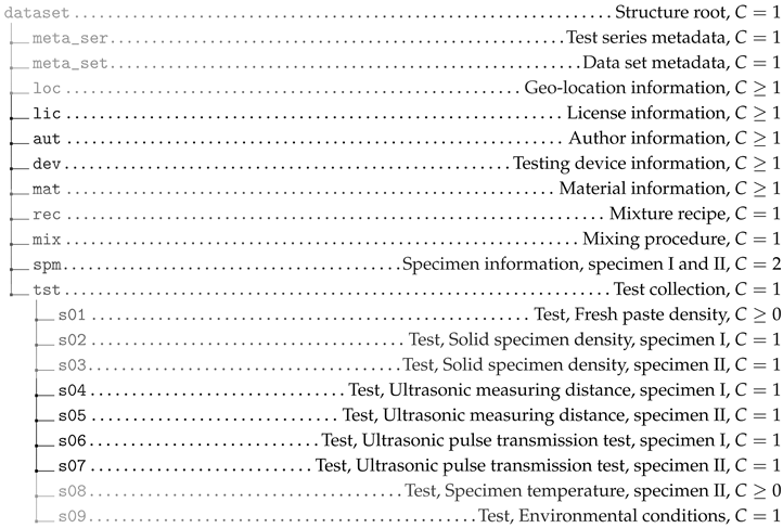
Substructures:
The substructures (e.g. dataset.meta_set, dataset.aut, dataset.s01) contain thematically related data elements, the atomic elements. The substructures are present in the data set either as a scalar substructure (cardinality , e.g. dataset.meta_set) or as an indexed substructure sequence (cardinality , e.g. dataset.dev). In substructure sequences, the composition of the data elements is identical. These only differ in the data stored in the fields of the respective data elements.
A common feature of all substructures and data elements are the fields object (e.g. dataset.spm.obj) and version (e.g. dataset.spm.ver). The object field contains a unique identifier representing the format of the substructure. The version field contains a tuple of two unsigned integers representing the version number of the structure format. By these two data fields, it is possible to make future adaptations and corrections visible and to ensure compatibility with analysis algorithms relying on a specific structure format.
Atomic elements:
The atomic elements form the lowest structural level. They are made up of several data fields and can, therefore, be regarded as complex data types. The composition of the data fields of these elements depends on their use. The three structure types defined below are used in the data sets of this study.
- Atomic data element (ADE): This element is mainly used to store numerical data (e.g. measurement data) and contains the fields tag (ADE.t), value type (ADE.vt), value (ADE.v), physical unit (ADE.u) and description (ADE.d). The field ADE.vt contains a data type descriptor and enables the correct interpretation of the value stored in the field ADE.v. The field ADE.u provides information about the physical unit of the value stored in ADE.v.
- Atomic attribute element (AAE): This element is used exclusively for storing metadata in the form of strings (character arrays) and contains the fields tag (AAE.t), value (AAE.v) and description (AAE.d). The AAE.v field can consist of either a single string or a sequence of strings.
- Atomic reference element (ARE): This element is used exclusively for referencing substructures and contains the fields tag (ARE.t), identifier (ARE.i), reference (ARE.r) and description (ARE.d). This element prevents the need to create copies of substructures used multiple times, for example, for a test specimen used in several consecutive tests. The field ARE.r contains a sequence of character strings that map the structure path to the referenced substructure (e.g. {’dataset.spm’}). The field ARE.i contains the unique numerical identifier of the referenced substructure. All referenceable substructures contain an ADE with the object name d01, whose field value (d01.v) contains the unique numerical identifier.
The fields tag and description are present in all three variants and contain the data element’s short name and the content’s description, respectively. A detailed illustration of the datasets’ structure elements of Test series 1, please find in Supplementary Figure 1 (see Supplementary Information Document, p.2). The datasets’ structure of the reference tests of Test series 5, Test series 6 and Test series 7, please find in Supplementary Figure 2 (see Supplementary Information Document, p.3). Application examples in section ‘Usage Notes’ p. 42 explain how to access the data in the data structure.
4. Technical Validation
This section is dedicated to validating the technical quality of the ultrasound measuring results. The validation aims to show that the signal data reproducibly reflects the underlying physical laws of sound propagation. For this purpose, the ultrasound measurement data from the datasets of Test series 5, Test series 6 and Test series 7 are used, since the properties of the materials used are known. The selected datasets and the analysis methods are detailed in subsection ‘Analysis Methods for the Technical Validation’, p. 27.
During the validation procedure, the ensemble average of signal sequences and the signal’s deviation from the ensemble average are estimated and displayed. The ensemble average represents the average signal response and is used to justify whether the signal data reflects the physical laws of sound propagation. The distribution of the deviations from the ensemble average provides information on the reproducibility of the ultrasound tests.
Due to measurement tolerances and procedural errors, the analysis results are not expected to accurately reproduce the literature-based predictions for the sound travel time also referred to as time-of-flight (ToF). However, those predictions should be within the estimated tolerance limits. The following effects and behavioural patterns should be evident in the analysis results.
- The sound travel time observed is within the tolerance range of literature-based estimates considering procedural and measuring errors.
- The relation between the sound travel time and the ultrasonic measuring distance is linear.
- The sound travel times of the reflections of the sound wave are odd integer multiples of the sound travel time of the first appearance of the sound wave.
- For all materials, the signal amplitudes decrease with increasing ultrasonic measuring distance.
- For air (an approximately ideal gas), the maximum amplitude of the first incoming sound wave and the maximum amplitudes of the reflections of this sound wave are decreasing linearly.
- Using the same test parameters, repeated test execution leads to similar results.
The graphical representations of the analysis results are summarized in the following list, sorted by test series and ultrasonic measuring distance.
-
Test series 5, reference tests on air, primary wave’ signal responseoct2tex.aird25v800Poct2tex.aird50v800Poct2tex.aird70v800P
-
Test series 6, reference tests on water, primary wave’ signal response
-
Test series 7, reference tests on aluminum cylinder, mm
The illustrations of the analysis results show that the predicted sound travel times can be read from the ensemble average M of the ultrasound signal sequences. They also show that almost all behavioural patterns listed above are met, with the exception of criterion No. 4.
According to criterion No. 4, a reciprocal relation between ultrasonic measuring distance D and the maximum signal amplitude of the first appearance of the sound wave is expected. The analysis results of the reference tests on air and water do not satisfy this expectation. For the reference tests on water, the maximum amplitude ( V) shown in Figure 12, p.40 ( mm) is larger than the maximum amplitude ( V) shown in Figure 8, p.36 ( mm). Furthermore, for the reference tests on air, the maximum amplitude of M seems to be independent of the ultrasonic measuring distance of D because the maximum amplitudes of ( V) in Figure 7, p.36 ( mm), Figure 8, p.36 ( mm) and Figure 9, p.37 ( mm) are almost equal. This contradictory behaviour is due to the automatic amplitude pre-amplification of the oscilloscope mentioned in subsection ‘Data Acquisition’, p. 25. Nevertheless, this criterion is met within the ensemble average of a signal sequence, since the maximum amplitudes of the reflections of the sound wave become smaller with increasing distance.
oct2tex.waterd70v800P
The analysis results for the aluminium cylinder are admittedly difficult to read. Particularly apparent becomes the fact mentioned in subsection ‘Experimental Setup’, p. 4 that the signal response of the secondary wave (shear wave) in Figure 14, p.41 is superimposed by the signal response of the primary wave (compression wave). Conversely, the same applies to the signal response of the primary wave shown in Figure 13, p.41. However, the sound travel time of the primary wave and the deviation from the ensemble average are readable.
The reproducibility of the ultrasound tests appears to be consistent. The minimum and maximum deviations are in the range of one-twentieth of the maximum amplitude of the ensemble average in all cases shown. Whether that is sufficient for a particular application can only be justified within the context of that application.
5. Usage Notes
This section describes how to access the data records’ content and to use the included binary datasets beneficially. The following explains how to extract the datasets from the data records’ compressed TAR archives, access the data structure in the datasets, and export and visualize signal data. The end of this section provides instructions to reproduce the analysis results illustrated in section ‘Technical Validation’ p. 35.. The descriptions below refer to the software provided by the author of this study (see section ‘Code Availability’ p. 44) but also to freely available open-source software.
Extracting datasets from compressed TAR archives:
After downloading the data records from the repository, the datasets are available in compressed TAR archives. To access the contained datasets, extract them from the archives first. Under Linux, the command line tool GNU tar is the simplest option. The following command decompresses and extracts the datasets from the TAR archives into the folder `ts1_dataset’ using the GNU bash[42] command line interface.
$ tar -xzf ts1_dataset.tar.xz
Accessing the data in a data set:
Since the datasets were written in the binary file format of GNU Octave, accessing them with this program is the most convenient option. Access to the structure elements’ data is possible using the following commands on the GNU Octave command line interface. Please note that lines beginning with a #–sign contain a comment which refers to the subsequent line.
>> # Load dataset and assign entire structure to variable ds
>> ds = load(’/path/to/dataset/file.oct’, ’dataset’).dataset;
>> # Assign the data of signal 12 from channel 1 to array s
>> s = ds.tst.s06.d13.v(:,12);
>> # Assign measurement unit of the signal data to variable u
>> u = ds.tst.s06.d13.u;
Please see section ‘Data Records’ p. 30 for an elaborate description of all structure elements. A general introduction[43] on using structures in GNU Octave is also available online.
Extracting data from a data set:
The access to the datasets’ measurement data and metadata is not limited to GNU Octave. To use the data stored in the datasets in other programs, they must be converted to other common file formats first. For this purpose, the script collection Data set exporter 1.1[44] is provided. The following examples show how to initialize that program, export ultrasound signal data and specimen temperature data as a comma-separated value file (CSV), and to convert the metadata into the JSON structure format or the format. Please note, that the function `init()’ must be called once before executing the other commands.
>> # (1) Initialize program ’Dataset Exporter’
>> init();
>> # (2) Load export settings into variable ES
>> ES = dsexporter_settings();
>> # (3) Define the output directory path ODP
>> ODP = ’/path/to/output/directory’;
>> # (4) Define the data set file path IFP
>> IFP = ’/path/to/dataset/dataset.oct’;
>> # (5) Export signal 10 from channel 1 to CSV file
>> dsexporter_sig2csv(ES, ODP, IFP, 1, 10);
>> # (6) Export specimen temperature data to a CSV file
>> dsexporter_tem2csv(ES, ODP, IFP, 1);
>> # (7) Export data set metadata to a JSON file
>> dsexporter_substruct2json(ES, ODP, IFP, ’meta_set’);
>> # (8) Export data set metadata to a LaTeX file
>> dsexporter_substruct2tex(ES, ODP, IFP, ’meta_set’);
Visualizing data from a data set:
Data visualization is one of the most important tasks in signal analysis. To simplify that task, the script collection Data set viewer 1.0[45] is provided. The following examples show how to initialize the program, plot signal and temperature data, and render a sequence of ultrasound signals into an MP4 video file.
>> # (1) initialize program ’Dataset Viewer’
>> init();
>> # (2) load display settings
>> VS = dsviewer_settings();
>> # (3) define data set input file path
>> IFP = ’/path/to/dataset/dataset.oct’;
>> # (4) define temporary directory to create MP4 videos
>> TMP = ’/path/to/temp’;
>> # (4) display signal 100 from channel 1, 2D plot
>> dsviewer_2d(IFP, VS, 1, 100);
>> # (5) plot all signals from channel 1, 3D plot
>> dsviewer_3d(IFP, VS, 1);
>> # (6) render MP4 video of all signals in data set
>> dsviewer_mp4(IFP, TMP, VS);
>> # (7) display temperature data from channel 1
>> dsviewer_tem(IFP, VS, 1);
Converting datasets to MatLAB’s binary file format:
Another widely used numerical computation program is MatLAB[46]. To use the datasets in MatLAB, it is necessary to convert the datasets into MatLAB’s binary file format first. The following example shows how to do this conversion using the GNU Octave command line interface.
>> # load dataset (GNU Octave’s binary format)
>> ds = load(’/path/to/dataset.oct’, ’dataset’).dataset;
>> # convert dataset to the MatLAB binary file format, version 6
>> save(’-v6’, ’dataset_matlabv6.mat’, ’ds’);
>> # convert dataset to the MatLAB binary file format, version 7
>> save(’-v7’, ’dataset_matlabv7.mat’, ’ds’);
Reproducing the analysis results:
The analysis results shown in section ‘Technical Validation’ p. 35 were compiled using GNU Octave command scripts. First, download the TAR archives of Test series 5[29], Test series 6[30] and Test series 7[31] from the repository and extract the datasets from the archives as described above. Second, download the command script archive[47] from the repository and extract the files from the archive into a working directory. See also section ‘Code Availability’ p. 44. Third, adjust the variables `r_ds.paths.dssrc’, `r_ds.paths.ts5oct’, `r_ds.paths.ts6oct’ and `r_ds.paths.ts7oct’ in function file `anadd_param.m’ such that they point to the folders containing the previously extracted datasets (*.oct) as shown in the example below.
# full path, parent dirctory of the subdirectories
# ’ts5_datasets’, ’ts6_datasets’, ’ts7_datasets’
r\_ds.paths.dssrc = /home/acme/science/data;
# test series 5 *.oct files, subdirectory name
r\_ds.paths.ts5oct = ’ts5_datasets’;
# test series 6 *.oct files, subdirectory name
r\_ds.paths.ts5oct = ’ts6_datasets’;
# test series 7 *.oct files, subdirectory name
r\_ds.paths.ts5oct = ’ts7_datasets’;
Finally, the commands listed below allow to reproduce the analysis results from the reference tests’ datasets using the GNU Octave command line interface.
>> # initialize program
>> anadd_init();
>> # compile results and export them to LaTeX text files
>> anadd_analyse();
6. Code Availability
All datasets referenced in this work were compiled from the raw data, consisting of text files, into the binary file format of GNU Octave using command scripts. Therefore, compiling the datasets is not necessary. Nevertheless, those scripts help to comprehend the details of the compilation process.
Further script collections are provided that simplify access to the binary datasets and make it easier to visualize the signal data therein. In addition, the script collection used to compile and reproduce the analysis results presented in section ‘Technical Validation’ p. 35 is supplied.
All script collections listed below were implemented and tested with GNU Octave on the Debian 11[48] (Linux) operating system. For extensibility and sustainable use, the program code provided is licensed under the MIT[49] license and made available on the repository[2] of Graz University of Technology. Usage examples for that script collections, please find in section ‘Usage Notes’ p. 42.
- Data set compiler 1.2[33] is a tool for compiling the raw data into binary datasets with a hierarchical data structure. In addition, this tool also contains the metadata databases used in the data set compilation process.
- Data set exporter 1.1[44] is a tool for exporting data from the binary datasets. The following file formats are supported: (1) comma-separated text format, (2) the JSON structure format, and (3) the text format of .
- Data set viewer 1.0[45] is a tool for visualizing data from the binary datasets. The following functions are supported: (1) 2D plots of ultrasonic signal data; (2) 2D plots of the temperature data of the specimens; (3) 3D plots of ultrasound signal sequences and (4) rendering ultrasound signal sequences to the MP4 format.
- The script collection[47] used to compile the analysis results for the technical validation.
- GNU Octave[41]: scientific programming language.
- GNU tar[39]: command line interface (CLI) tool to handle TAR archives.
- Gzip[40]: CLI tool to handle ZIP archives.
- ffmpeg[50]: CLI tool to create and manipulate MPEG video files.
- shasum[51]: CLI tool to print or check SHA checksums. This tool is only needed to compile the binary datasets.
This open-source software is available for Linux and other operating systems (e.g. Microsoft Windows or MacOS). For Microsoft Windows users, using the freely available software 7-zip[52] is suggested instead of GNU tar and Gzip.
Author Contributions
J. Harden designed the experimental study, conducted all laboratory tests, collected and prepared the data, compiled the datasets and published the data records. The software packages (script collections) provided were also conceived, implemented, tested, and made available by J. Harden. Furthermore, the entire content of this manuscript was conceived, designed and written by J. Harden.
Acknowledgments
Supported by TU Graz Open Access Publishing Fund.
Conflicts of Interest
The authors declare no competing interests.
References
- creativecommons.org. Creative Commons – Attribution 4.0 International, SPDX short identifier: CC-BY-4.0. https://creativecommons.org/licenses/by/4.0/legalcode, (accessed on 2025). (accessed on 2025).
- re3data.org: TU Graz Repository; editing status 2024-02-13; re3data.org – Registry of Research Data Repositories. (accessed on 2024). [CrossRef]
- Harden, J. Ultraschall-Puls-Transmissionsverfahren: Automatisierte Drift-Erkennung in Signalreihen von Zementleimen im frühen Stadium der Hydratation 2023. [CrossRef]
- Harden, J. Ultrasonic through-transmission method: Characterization and detection of the electromagnetic disturbances caused by pulse excitation observed in combined compression and shear wave measurements of cement paste 2023. [CrossRef]
- Maruyama, I.; Igarashi, G. Cement Reaction and Resultant Physical Properties of Cement Paste. Journal of Advanced Concrete Technology 2014, 12, 200–213. [Google Scholar] [CrossRef]
- EurocodeApplied.com. Table of concrete design properties according to Eurocode 2 (EN1992-1-1). 2024. https://eurocodeapplied.com/design/en1992/concrete-design-properties, (accessed on 2024). (accessed on 2024).
- Illston, J.; Domone, P. Construction Materials: Their Nature and Behaviour, 3 ed.
- Generalization of Abrams’ law. Cement and Concrete Research 1996, 26, 933–942. [CrossRef]
- Kargari, A.; Eskandari-Naddaf, H.; Kazemi, R. Effect of cement strength class on the generalization of Abrams’ law. Structural Concrete. [CrossRef]
- Determining the water–cement ratio, cement content, water content and degree of hydration of hardened cement paste: Method development and validation on paste samples. Cement and Concrete Research 2009, 39, 957–965. [CrossRef]
- Haach, V.G.; Vasconcelos, G.; Lourenço, P.B. Influence of aggregates grading and water/cement ratio in workability and hardened properties of mortars. 2011; 25, 2980–2987. [Google Scholar]
- The microstructure development during bleeding of cement paste: An NMR study. Cement and Concrete Research 2019, 125, 105866. [CrossRef]
- Wave propagation based monitoring of concrete curing using piezoelectric materials: Review and path forward. NDT & E International 2018, 99, 50–63. [CrossRef]
- Ruck, H.J.; Große, C.; Reinhardt, H.W. Automatisierung der Ultraschallmessung von Frischbeton 2021.
- Ballas, R. The Piezoelectric Effect – an Indispensable Solid State Effect for Contemporary Actuator and Sensor Technologies. Journal of Physics: Conference Series 2021, 1775, 12. [Google Scholar] [CrossRef]
- Yoshida, S. Fundamentals of Acoustic Waves and Applications, 1 ed.; Synthesis Lectures on Wave Phenomena in the Physical Sciences, Springer Cham; pp. 65–85,87–121. [CrossRef]
- Roeser, W. Thermoelectric Thermometry. Journal of Applied Physics 1940, 11, 388–407. [Google Scholar] [CrossRef]
- Smartmote.; Universität Stuttgart. FreshCon-Duo 4.00 User Manual. https://smartmote.de/joomla/images/PDF/Anleitung-FreshCon-V4-_0.pdf, (accessed on 2012).
- EVIDENT. Contact Transducers. https://www.olympus-ims.com/en/ultrasonic-transducers/contact-transducers/#!cms[focus]=cmsContent10862, (accessed on 2025).
- picoScope. PicoScope 4262 Specifications. https://www.picotech.com/oscilloscope/4262/picoscope-4262-specifications, (accessed on 2023).
- National Instruments. cDAQ-9171 Specifications. https://www.ni.com/docs/de-DE/bundle/cdaq-9171-specs/page/specs.html, (accessed on 2025).
- National Instruments. NI-9217 Specifications. https://www.ni.com/docs/de-DE/bundle/ni-9210-specs/page/specs.html, (accessed on 2024).
- Sartorius. BP12000S Specifications. 1995. https://www.dataweigh.com/device/sartorius-lab/bp-series/bp12000s#specifications, (accessed on 1995).
- Sartorius. LC2200P Specifications. 2002. https://www.dataweigh.com/device/sartorius-lab/lc-series/lc2200p#specifications, (accessed on 2002).
- Mettler Toledo. Precision Balance MS16001L/02 Specifications. 2023. https://www.mt.com/my/en/home/phased_out_products/Laboratory_Weighing_Solutions/precision-balances/MS16001L-02.html, (accessed on 2023).
- Helios-Preisser. METROLOGY CATALOGUE 2023/2024 – DIGIMET 1320. https://www.helios-preisser.com/fileadmin/user_upload/_assets/Downloads/Catalog_HP_EN_2023.pdf, (accessed on 2023).
- Testo. testo 177-T4 Short Instruction Manual. https://static.testo.com/image/upload/Instruction-manual-and-Software/Instruction-manuals/testo-177-short-instruction-manual-7396.pdf, (accessed on 2011).
- Testo. testo 177-H1 Short Instruction Manual. https://static.testo.com/image/upload/Instruction-manual-and-Software/Instruction-manuals/testo-177-short-instruction-manual.pdf, (accessed on 2011).
- Harden, J. Ultrasonic Pulse Transmission Tests: Datasets – Test Series 5, Reference Tests on Air. 2023.
- Harden, J. Ultrasonic Pulse Transmission Tests: Datasets – Test Series 6, Reference Tests on Water. 2023.
- Harden, J. Ultrasonic Pulse Transmission Tests: Datasets – Test Series 7, Reference Tests on Aluminium Cylinder. 2025.
- LibreOffice – The Document Foundation. LibreOffice. 2020. https://downloadarchive.documentfoundation.org/libreoffice/old/7.0.4.2/, (accessed on 2020).
- Harden, J. Ultrasonic Pulse Transmission Tests: Data set compiler. 2025. (accessed on 2025). TU Graz Repository. [CrossRef]
- The Engineering ToolBox. Air – Speed of Sound vs. Temperature. 2003. https://www.engineeringtoolbox.com/air-speed-sound-d_603.html, (accessed on 2003).
- The Engineering ToolBox. Water – Speed of Sound vs. Temperature. 2004. https://www.engineeringtoolbox.com/sound-speed-water-d_598.html, (accessed on 2004).
- Garrett, S.L. Understanding Acoustics: An Experimentalist’s View of Sound and Vibration, 2 ed.; Graduate Texts in Physics, 2020.
- The Engineering ToolBox. Aluminum Alloys – Mechanical Properties. 2008. https://www.engineeringtoolbox.com/properties-aluminum-pipe-d_1340.html, (accessed on 2008). (accessed on 2008).
- Harden, J. Ultrasonic Pulse Transmission Tests: Datasets – Test Series 1, Cement Paste at Early Stages. 2023.
- Free Software Foundation, Inc. tar(1) – Linux man page. 2010. https://linux.die.net/man/1/tar, (accessed on 2010).
- Free Software Foundation, Inc. GNU Gzip. 2020. https://www.gnu.org/software/gzip/, (accessed on 2020).
- Eaton, J. GNU Octave. 2021. https://octave.org/news/release/2021/02/20/octave-6.2.0-released.html, (accessed on 2021).
- Free Software Foundation, Inc. bash(1) – Linux man page. 2009. https://linux.die.net/man/1/bash, (accessed on 2009).
- docs.gnuoctave.org. GNU Octave Documentation, 6. docs.gnuoctave.org. GNU Octave Documentation, 6.1 Structures. 2021. https://docs.octave.org/v6.2.0/Structures.html, (accessed on 2021).
- Harden, J. Ultrasonic Pulse Transmission Tests: Dataset Exporter. 2023. (accessed on 2023). TU Graz Repository. [CrossRef]
- Harden, J. Ultrasonic Pulse Transmission Tests: Dataset Viewer. 2023, (accessed on 2023). TU Graz Repository. [CrossRef]
- MathWorks. MatLAB – Math, Graphics, Programming. 2024. https://mathworks.com/products/matlab.html, (accessed on 2024).
- Harden, J. Source code for: Experimental study on cement paste using the ultrasonic pulse transmission method. 2024, (accessed on 2024). TU Graz Repository. [CrossRef]
- Debian. Debian – The universal operating system. 2023. https://www.debian.org/index.en.html, (accessed on 2023).
- Massachusetts Institute of Technology. The MIT License, Version N/A, SPDX short identifier: MIT. https://opensource.org/license/mit/, (accessed on 2025).
- ffmpeg.org. FFmpeg – A complete, cross-platform solution to record, convert and stream audio and video. 2024. https://www.ffmpeg.org/, (accessed on 2024).
- Free Software Foundation, Inc. sha256sum(1) – Linux man page. 2010. https://linux.die.net/man/1/sha256sum, (accessed on 2010).
- Pavlov, I. 7-zip download. 2024. https://www.7-zip.org/download.html, (accessed on 2024).
Figure 1.
The experimental study – procedural components and workflow.
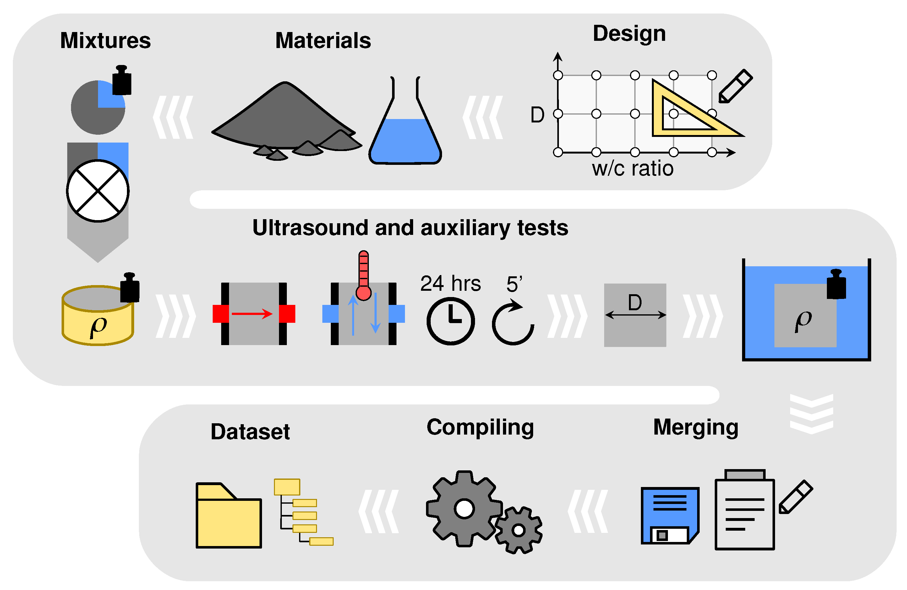
Figure 2.
Schematic representation of the ultrasound testing device FreshConDUO. Legend: …high-voltage pulse; …analogue signal; ⊲ …trigger impulse.
Figure 2.
Schematic representation of the ultrasound testing device FreshConDUO. Legend: …high-voltage pulse; …analogue signal; ⊲ …trigger impulse.
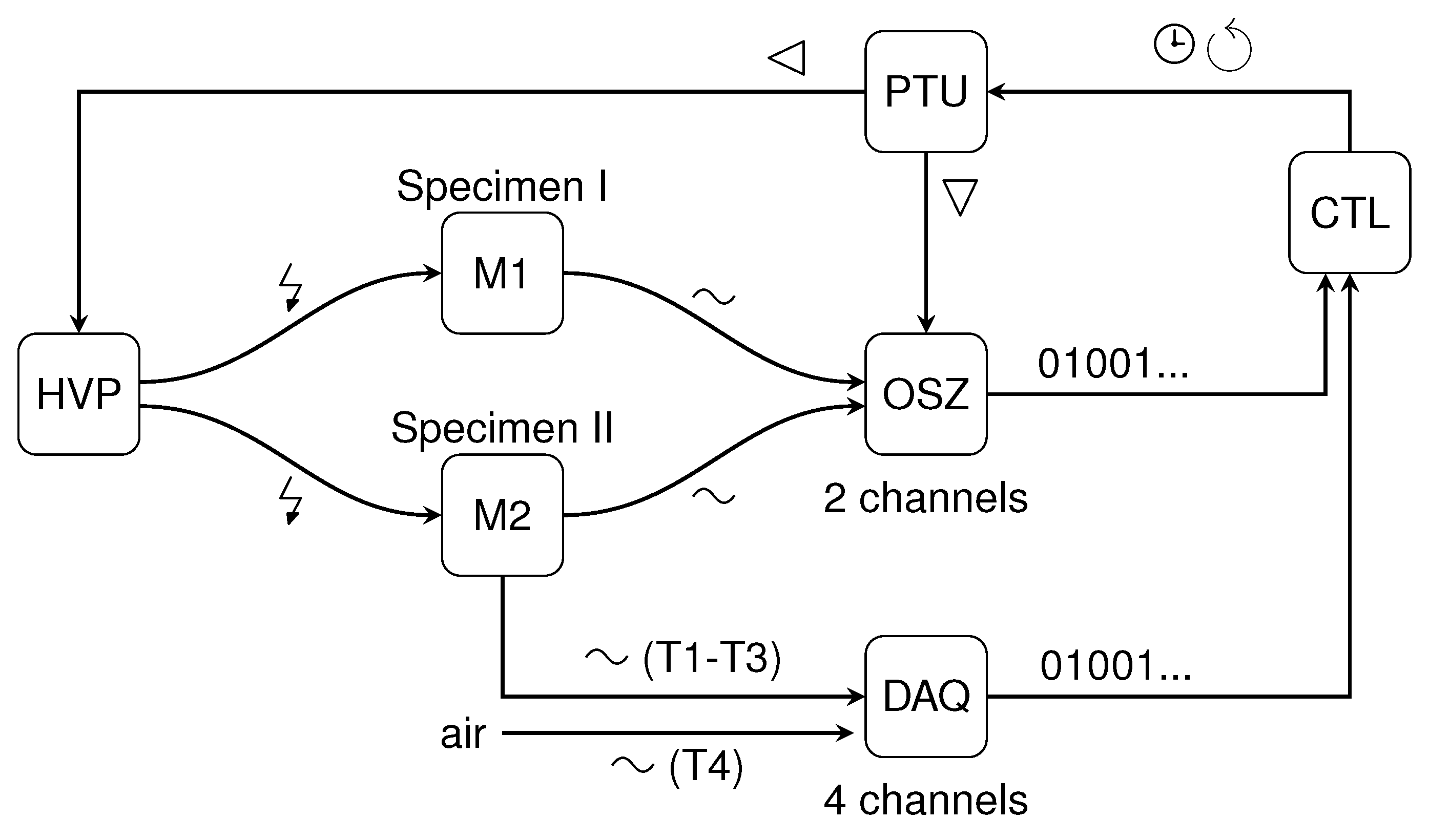
Figure 3.
Schematic view of the ultrasound testing device’ mould configuration. Note: mould M1 and mould M2 shown in Figure 2, p.5 are, except the built-in ultrasonic contact probes, identically constructed. With respect to the ultrasonic measuring distance D, one of the four mould variants (Mould-25, Mould-50, Mould-70a, Mould-70b) was chosen. The material ID’s (e.g. m11) mentioned in the legend refer to the materials listed in Table 6, p.12.
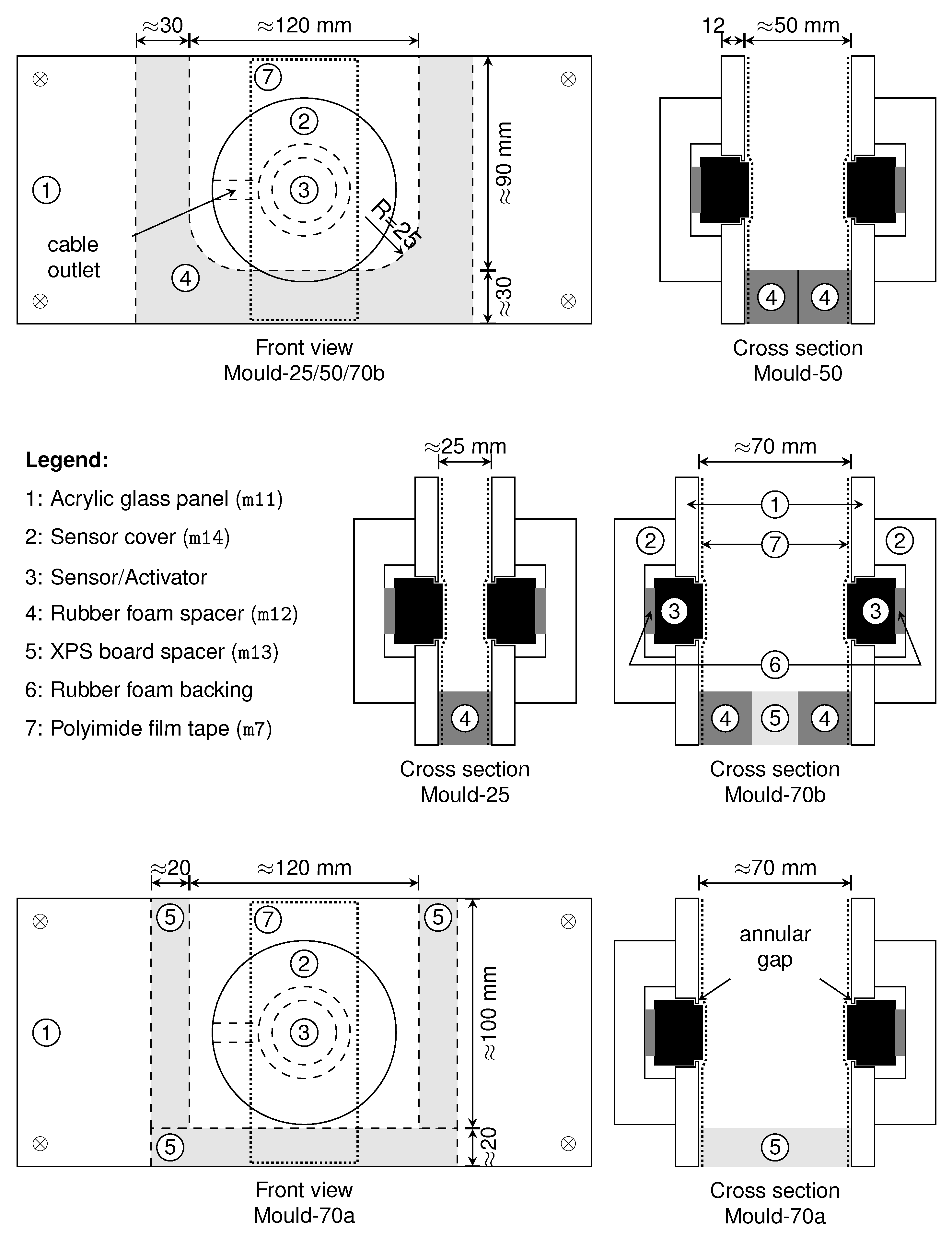
Figure 4.
Thermocouple placement schema. Locations inside and outside of mould M2.
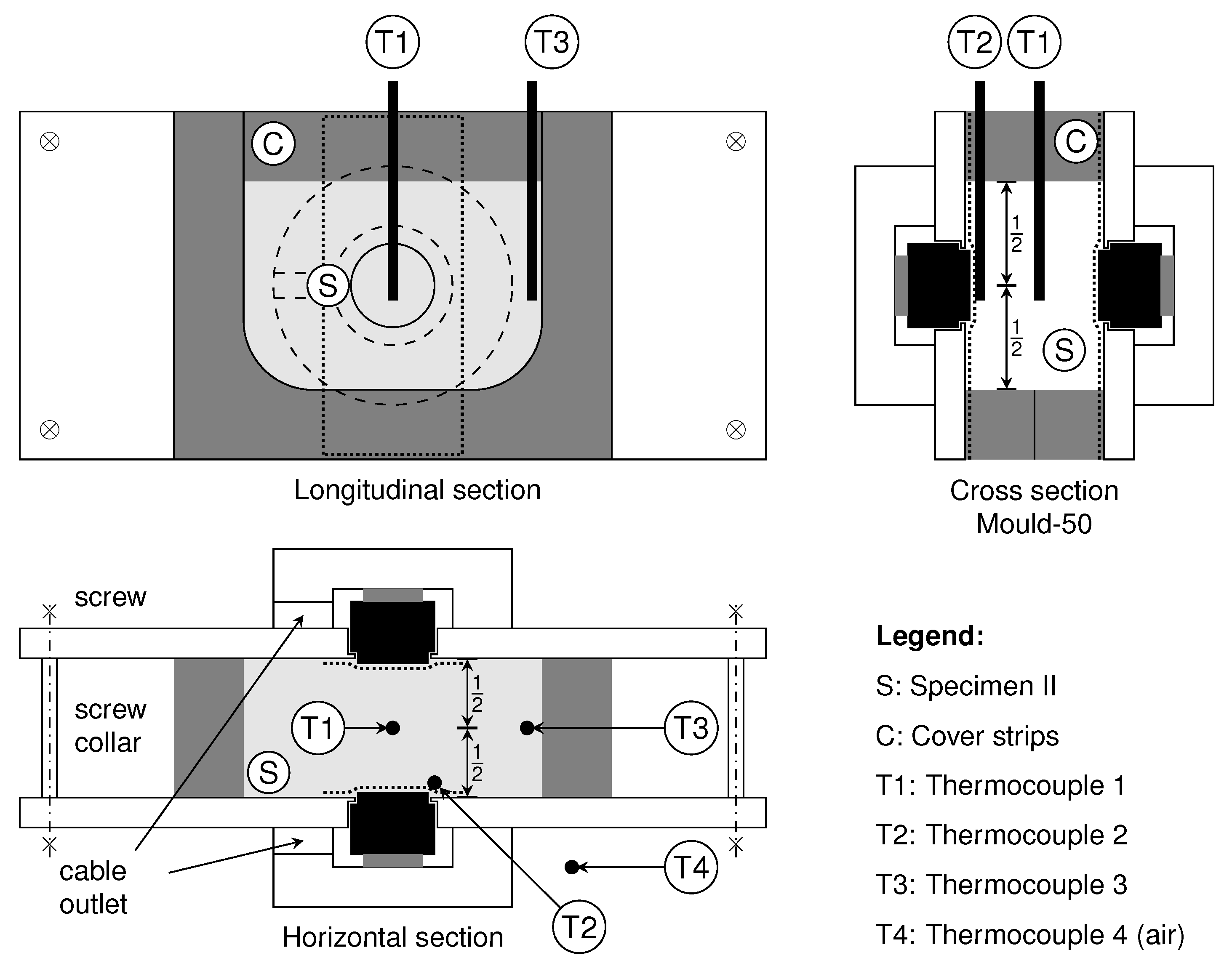
Figure 5.
The testing process workflow of a test run in Test series 1.
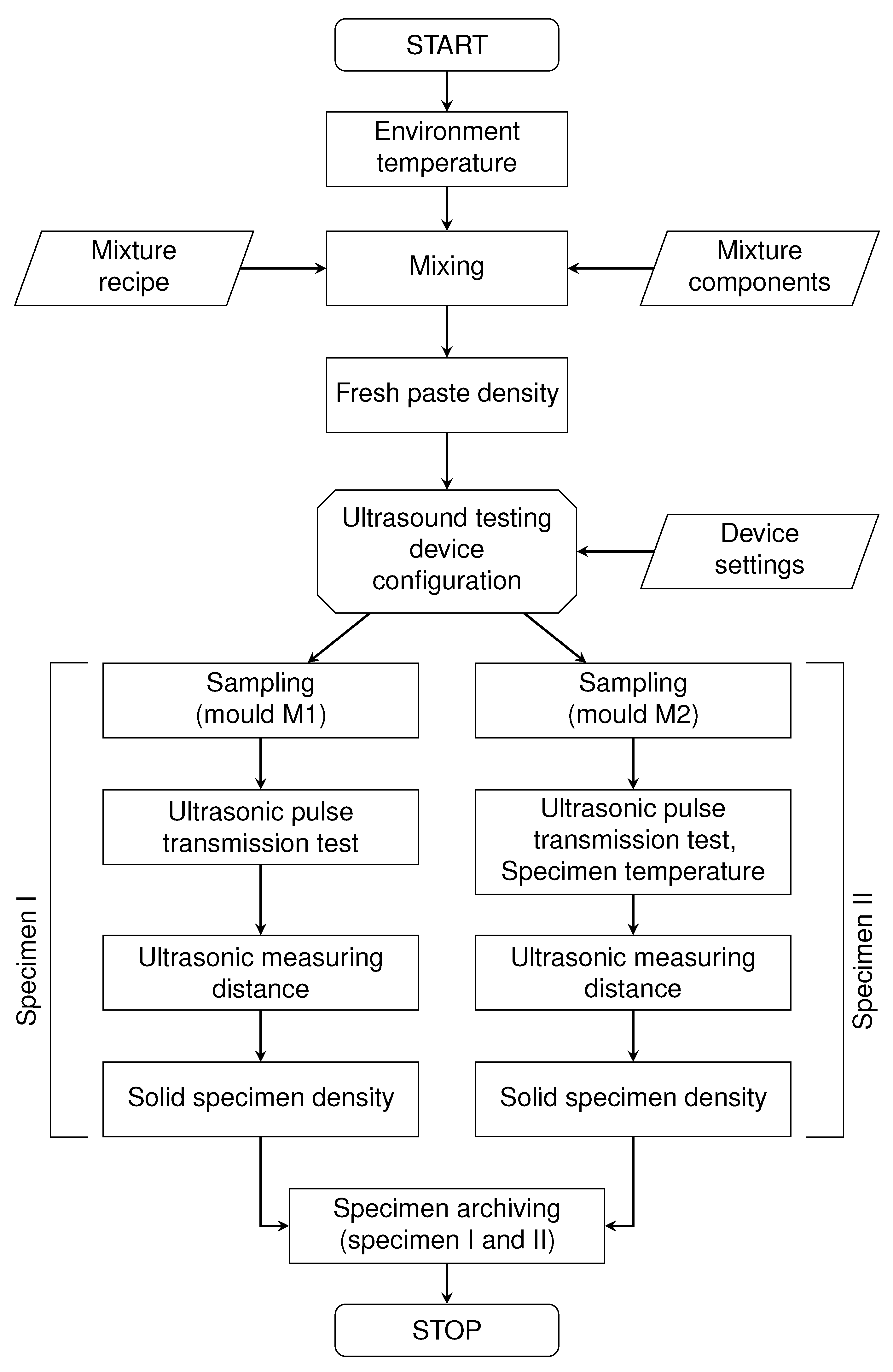
Figure 6.
Schematic representation of the data processing workflow. Data acquisition, data collection and data set compilation.
Figure 6.
Schematic representation of the data processing workflow. Data acquisition, data collection and data set compilation.
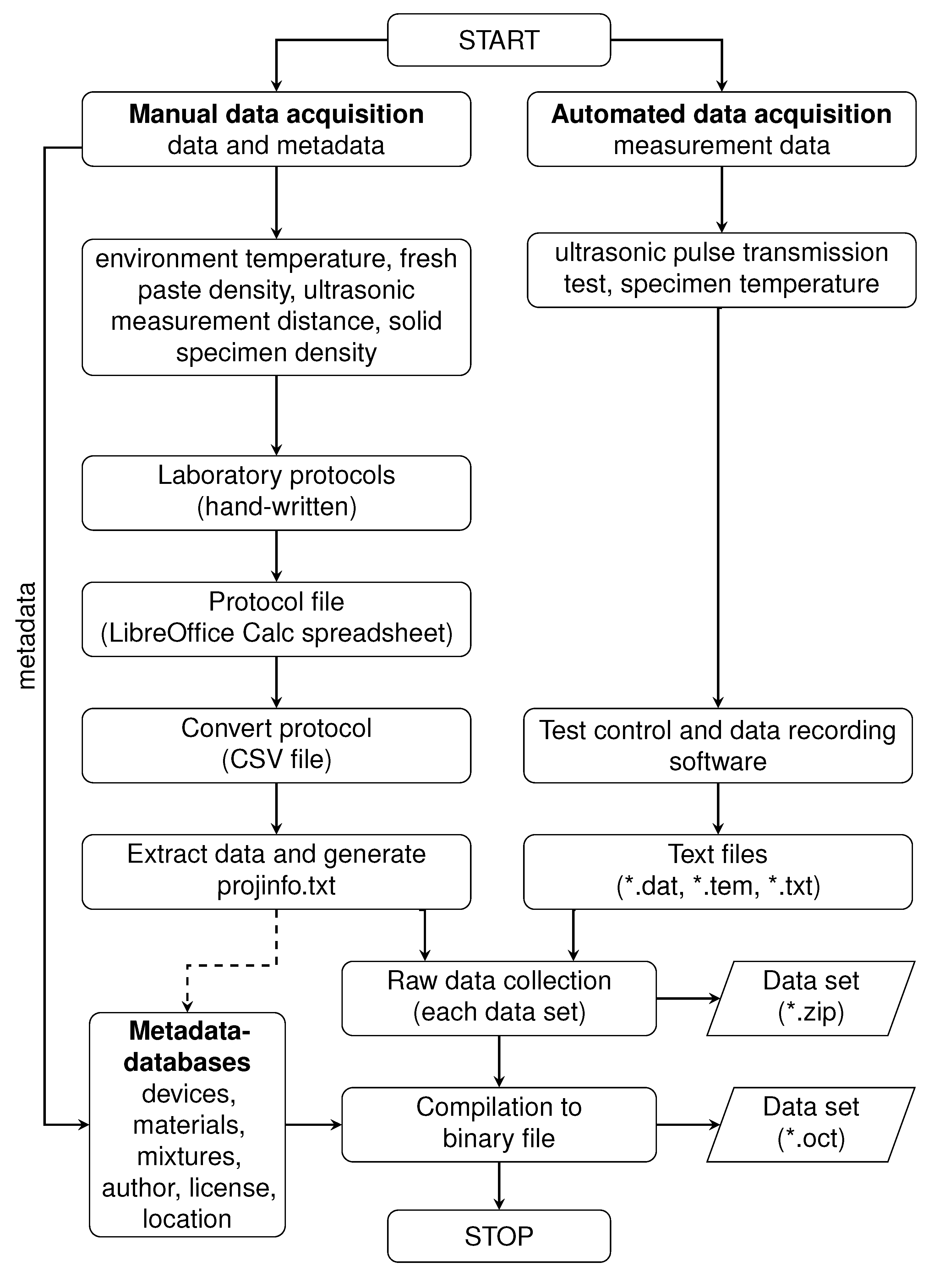
Figure 7.
Test series 5, reference tests on air – primary wave, mm. (a) Ensemble average M. (b) Deviation from ensemble average R.
Figure 7.
Test series 5, reference tests on air – primary wave, mm. (a) Ensemble average M. (b) Deviation from ensemble average R.
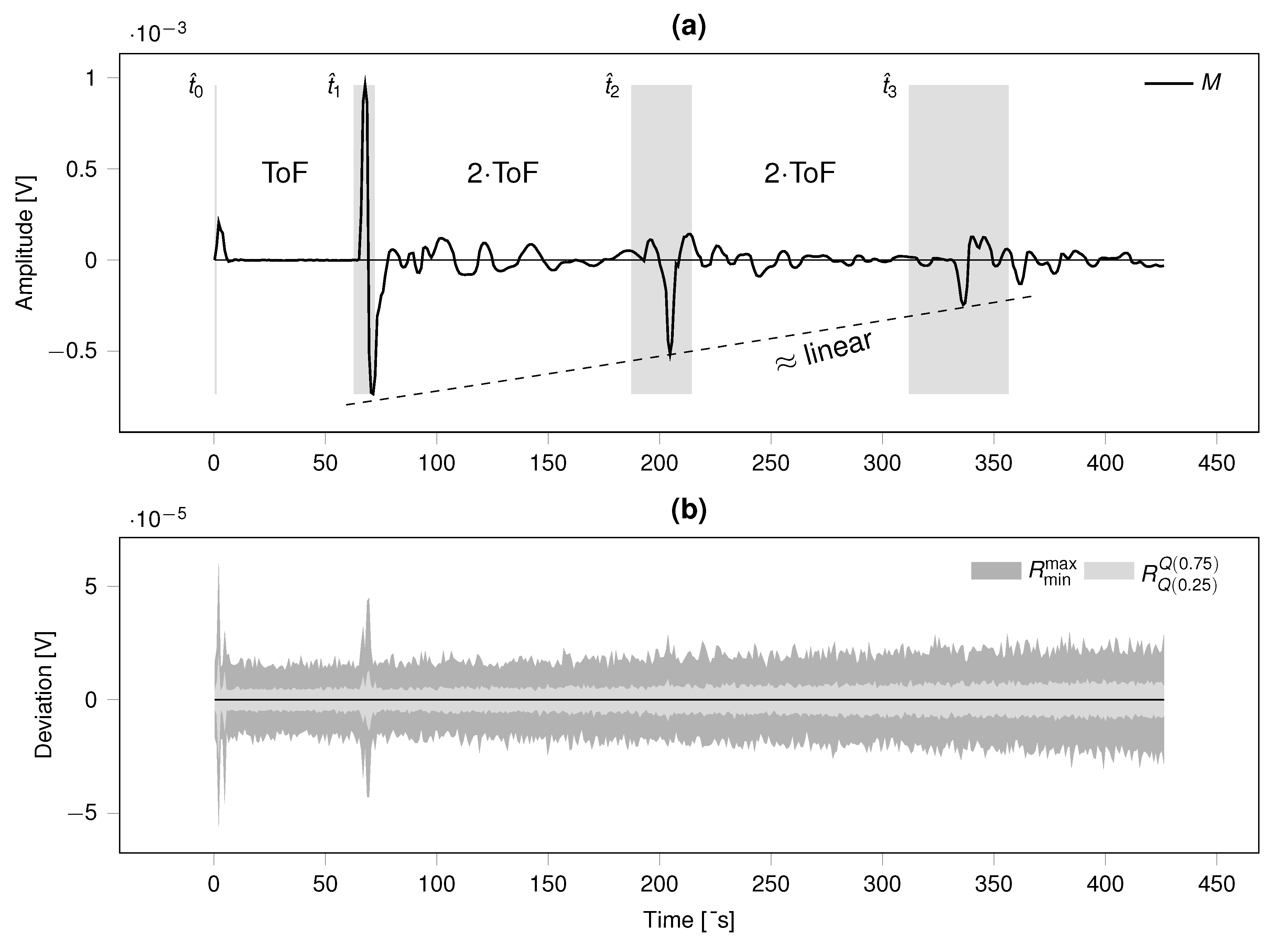
Figure 8.
Test series 5, reference tests on air – primary wave, mm. (a) Ensemble average M. (b) Deviation from ensemble average R.
Figure 8.
Test series 5, reference tests on air – primary wave, mm. (a) Ensemble average M. (b) Deviation from ensemble average R.
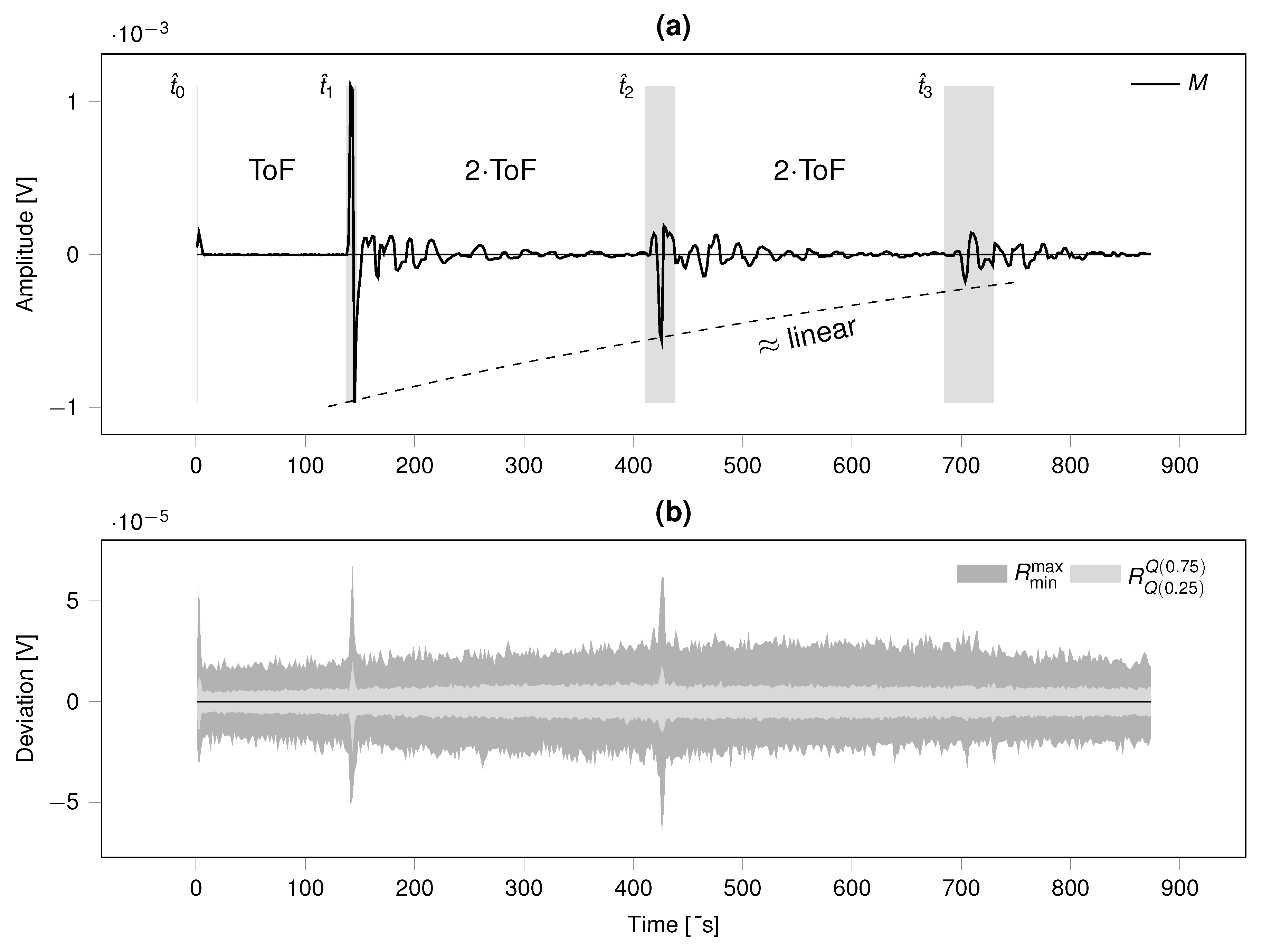
Figure 9.
Test series 5, reference tests on air – primary wave, mm. (a) Ensemble average M. (b) Deviation from ensemble average R.
Figure 9.
Test series 5, reference tests on air – primary wave, mm. (a) Ensemble average M. (b) Deviation from ensemble average R.
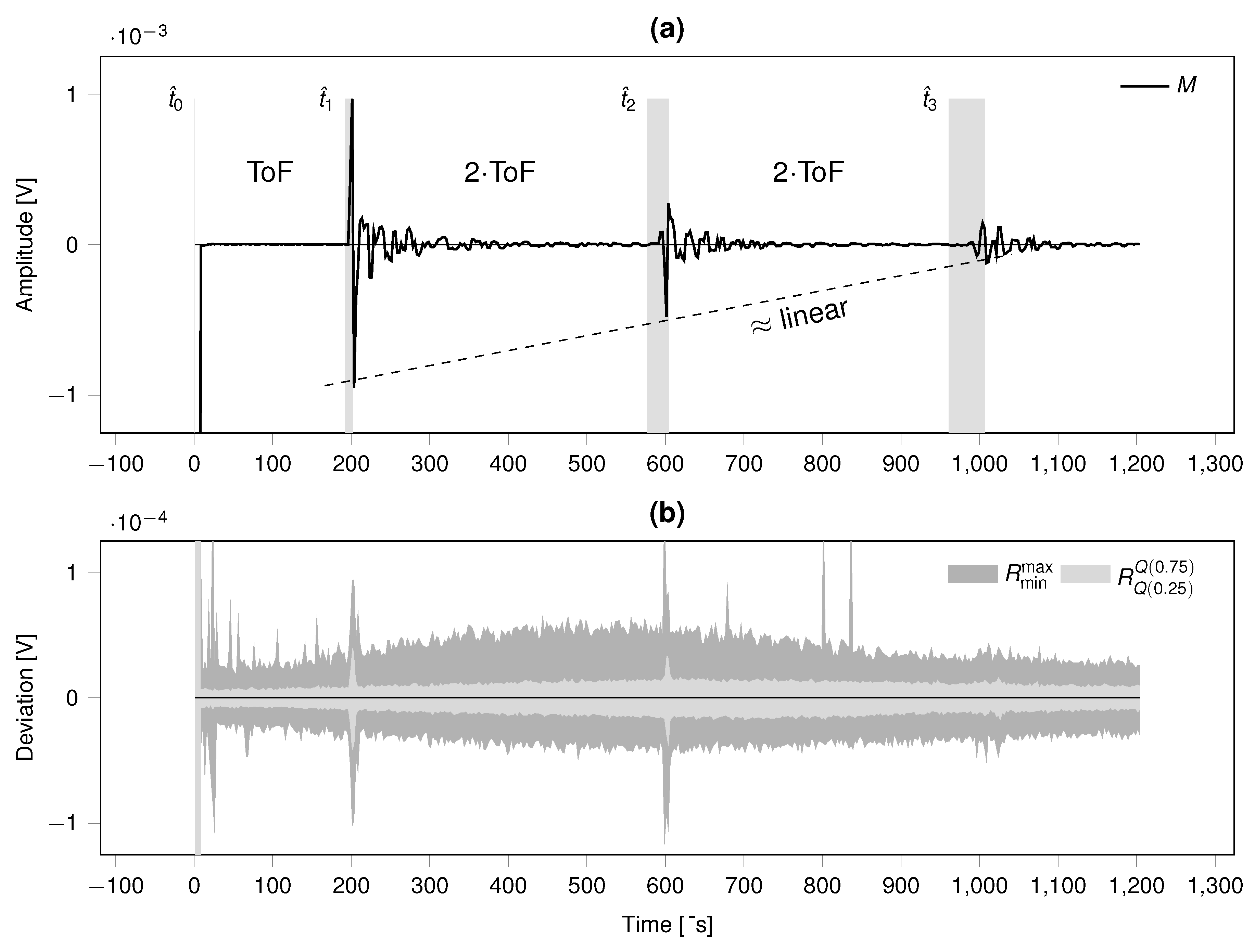
Figure 10.
Test series 6, reference tests on water – primary wave, mm. (a) Ensemble average M. (b) Deviation from ensemble average R.
Figure 10.
Test series 6, reference tests on water – primary wave, mm. (a) Ensemble average M. (b) Deviation from ensemble average R.
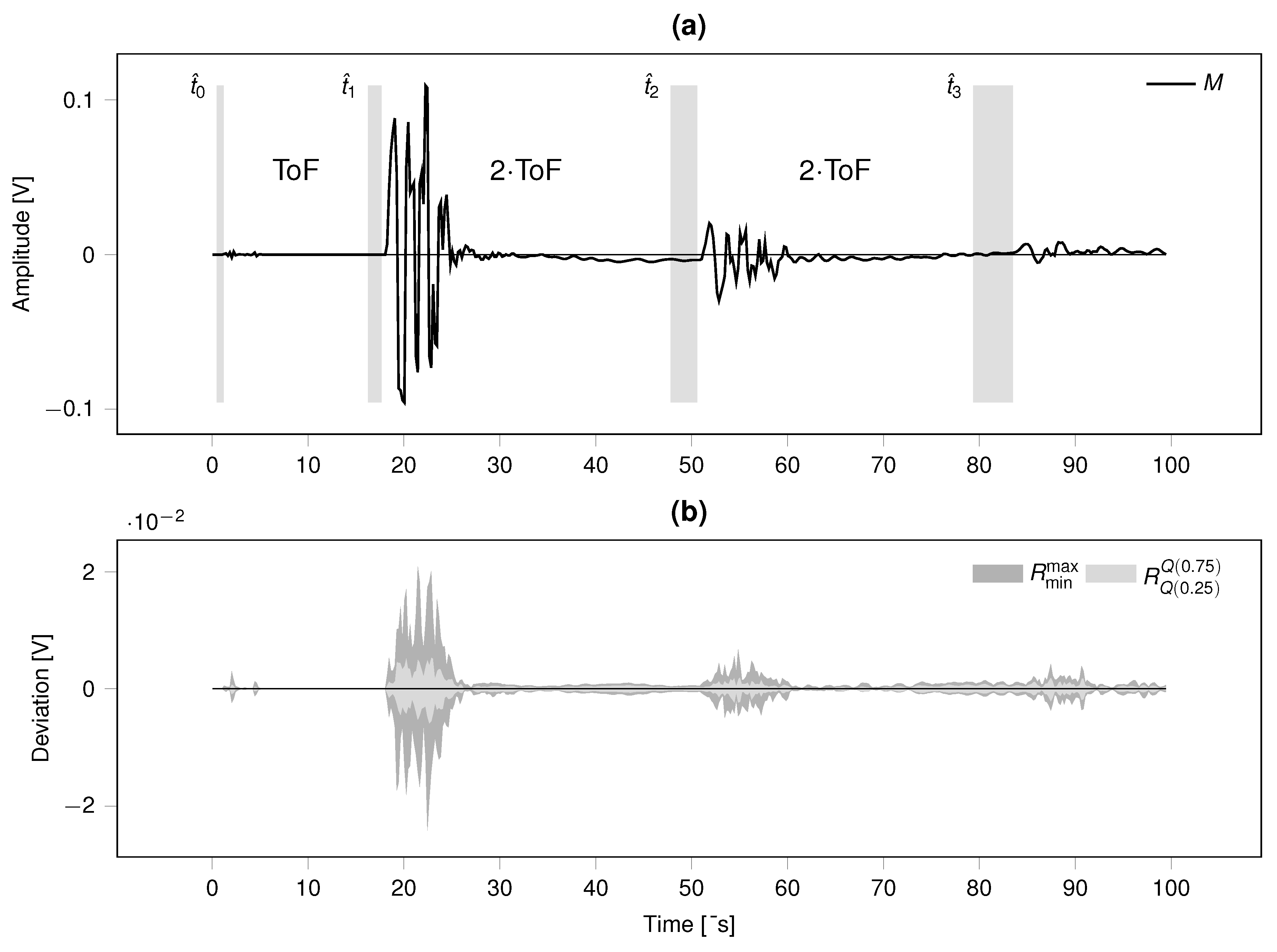
Figure 11.
Test series 6, reference tests on water – primary wave, mm. (a) Ensemble average M. (b) Deviation from ensemble average R.
Figure 11.
Test series 6, reference tests on water – primary wave, mm. (a) Ensemble average M. (b) Deviation from ensemble average R.
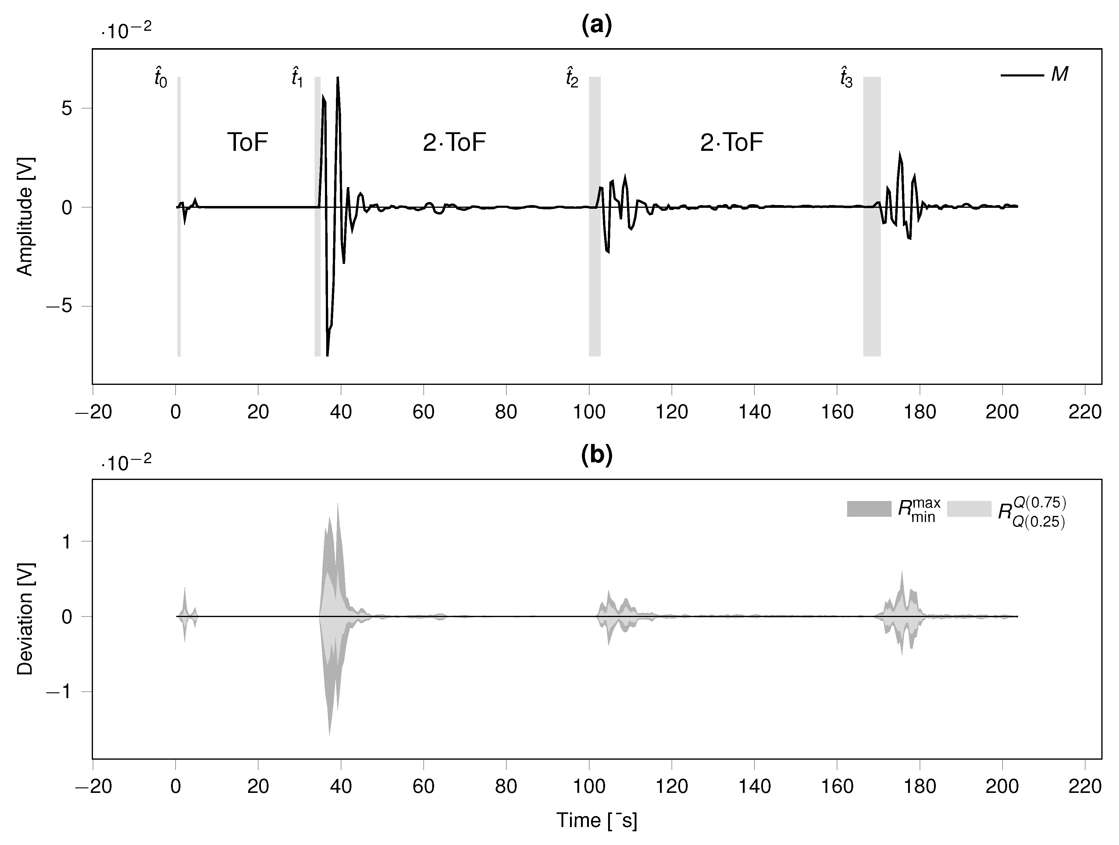
Figure 12.
Test series 6, reference tests on water – primary wave, mm. (a) Ensemble average M. (b) Deviation from ensemble average R.
Figure 12.
Test series 6, reference tests on water – primary wave, mm. (a) Ensemble average M. (b) Deviation from ensemble average R.
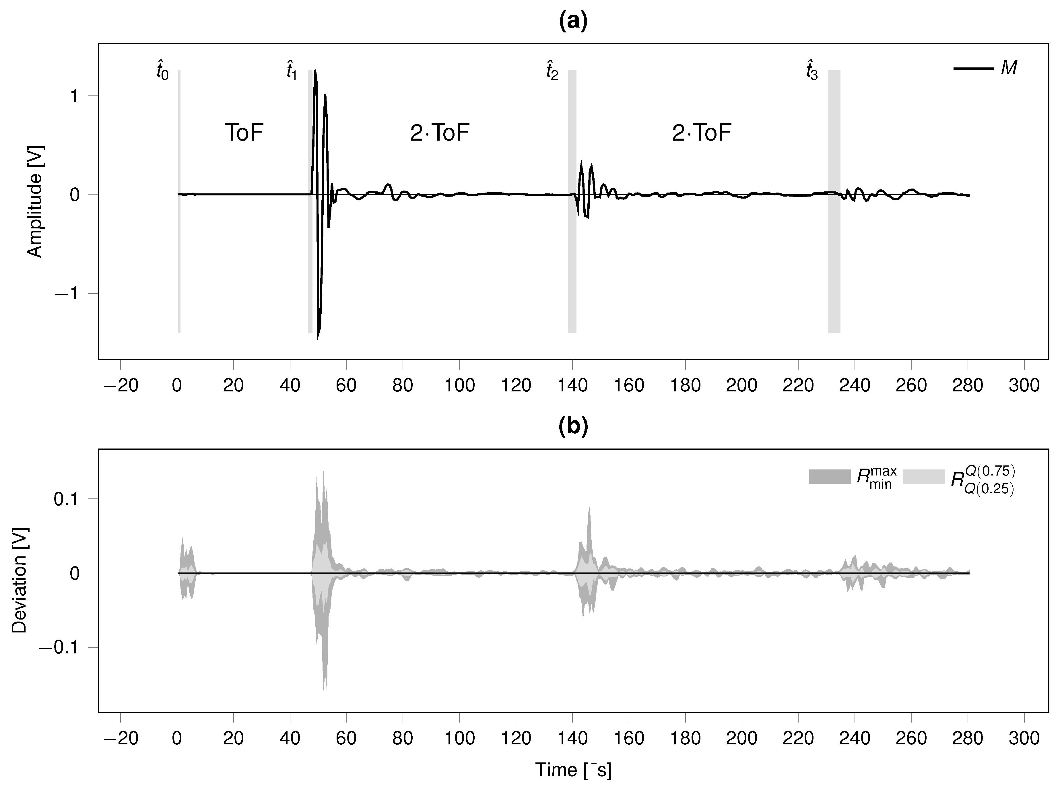
Figure 13.
Test series 7, reference tests on aluminum cylinder – primary wave, mm. (a) Ensemble average M. (b) Deviation from ensemble average R.
Figure 13.
Test series 7, reference tests on aluminum cylinder – primary wave, mm. (a) Ensemble average M. (b) Deviation from ensemble average R.
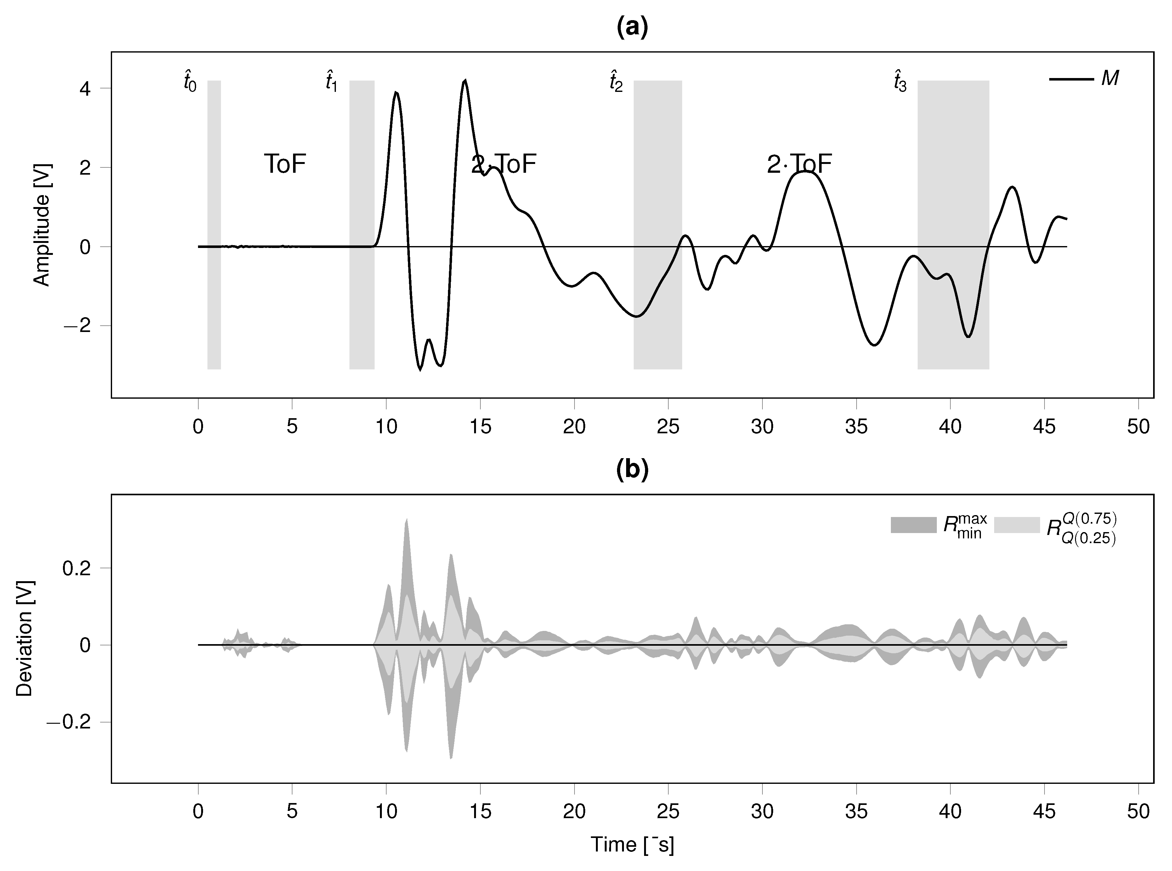
Figure 14.
Test series 7, reference tests on aluminum cylinder – secondary wave, mm. (a) Ensemble average M. (b) Deviation from ensemble average R.
Figure 14.
Test series 7, reference tests on aluminum cylinder – secondary wave, mm. (a) Ensemble average M. (b) Deviation from ensemble average R.
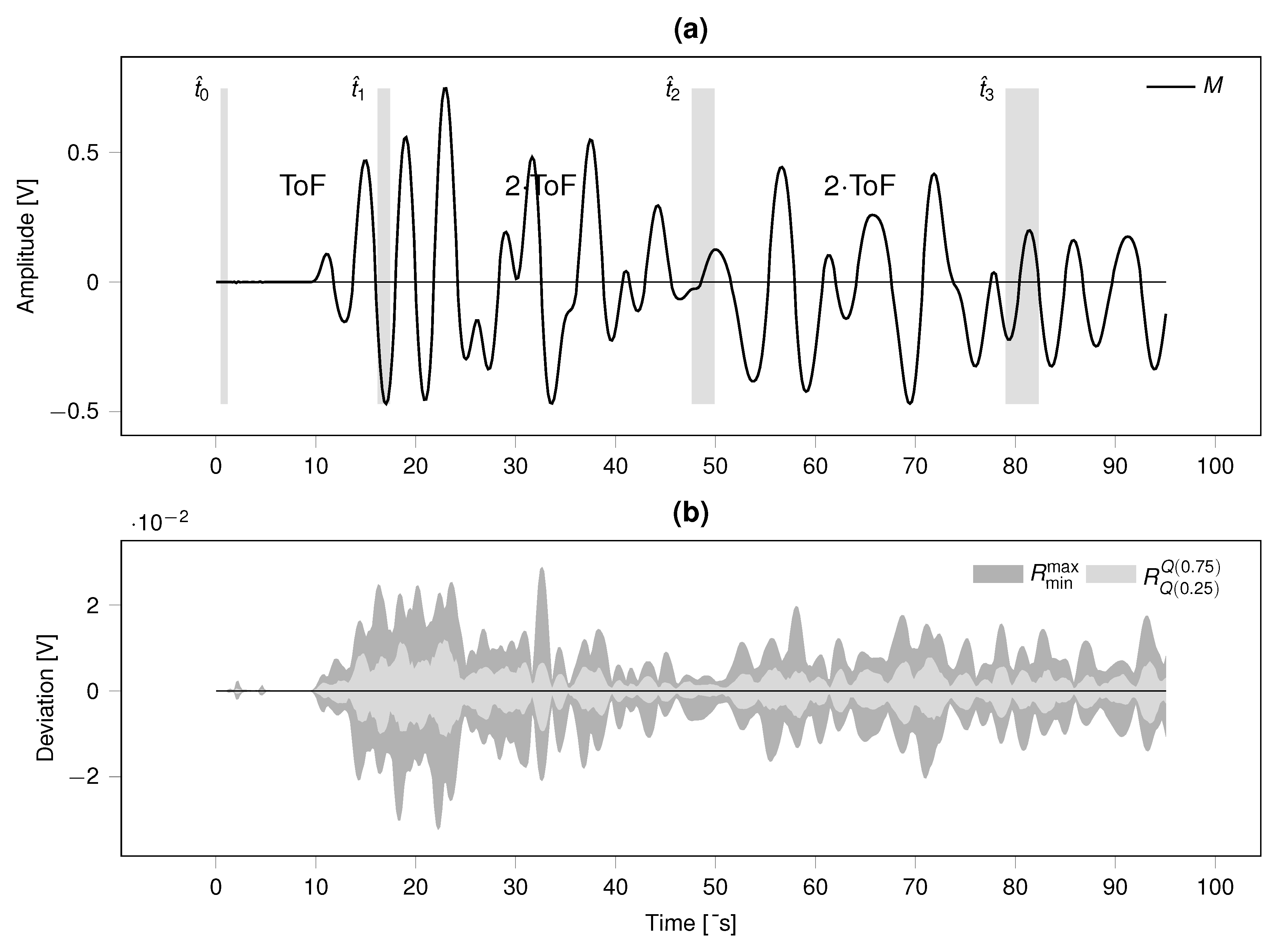
Table 1.
Testing devices. Legend: DID …unique device identifier.
| DID | Name | Vendor | Model, Type |
|---|---|---|---|
| d01 | Signal cable 1 | N/A | BNC, |
| d02 | Signal cable 2 | N/A | BNC, |
| d03 | Signal cable 3 | N/A | BNC, |
| d04 | Signal cable 4 | N/A | BNC, |
| d09 | Thermocouple | RS components | probe type T |
| d10 | Oscilloscope | picoScope | PS-4262 |
| d11 | Temperature DAQ | NationalInstruments | cDAQ-9171, NI-9217,probes: d09 |
| d12 | Pulse generator | piezosystems Jena | HVP-1000 |
| d13 | Pulse trigger unit | SmartMote | SmartPULSE, PTM v1.6 |
| d14 | Activator I | Olympus IMS | V101-RB[19] |
| d15 | Sensor I | Olympus IMS | V101-RB[19] |
| d16 | Activator II | Olympus IMS | V150-RB[19] |
| d17 | Sensor II | Olympus IMS | V150-RB[19] |
| d20 | Mold-25 | SmartMote | mm |
| d21 | Mold-50 | SmartMote | mm |
| d22 | Mold-70a | SmartMote | mm |
| d23 | Mold-70b | SmartMote | mm |
| d24 | Electronic balance | Sartorius | BP12000S |
| d25 | Electronic balance | Sartorius | LC2200P |
| d26 | Electronic balance | Mettler Toledo | MS16001L |
| d27 | Sliding caliper | Helios-Preisser | DIGI-MET 1320 |
| d28 | Compulsory mixer | Hobart | N50-619 |
| d29 | Graduated beaker | N/A | volume 1000 cm3 |
| d30 | Steel washer M12 | N/A | DIN 125,DIN EN ISO 7089 |
| d31 | Thermocouple | RS components | probe type K |
| d32 | Temperature DAQ | Testo GmbH | Testo 177-T4,probes: d31 |
| d33 | Temperature logger | Testo GmbH | Testo 177-H1 |
| d34 | Trowel | N/A | straight edges |
| d35 | Mold-90 | SmartMote |
Table 2.
Measuring device specifications. Legend: DID …unique device identifier.
| DID | Name, Specification | Value, Unit |
|---|---|---|
| d10 | picoScope PS-4262[20] | — |
| vertical, rise time (calculated) | 70 ns | |
| vertical, rise time ( mV) | ns | |
| vertical, resolution | 16 bits | |
| vertical, input sensitivity (10 divisions) | V | |
| vertical, input ranges (11 ranges) | V | |
| vertical, input characteristic, resistance | M | |
| vertical, input characteristic, capacity | pF | |
| vertical, DC acc. (% of full scale) | % | |
| vertical, DC acc., ( mV) | % | |
| horizontal, sampling rate | 10 MS/s | |
| horizontal, timebase accuracy | ppm | |
| horizontal, sample jitter (RMS) | ps | |
| d11 | National Instruments cDAQ-9171[21],NI-9217[22] | — |
| vertical resolution | 24 bits | |
| thermocouple probe (Table 1, p.8, d09) | type T | |
| accuracy (C), typical | ∘C | |
| accuracy (C), maximum | ∘C | |
| d24 | Sartorius BP12000S[23] | — |
| resolution ( g) | g | |
| linearity | g | |
| range capability | single (fixed) | |
| d25 | Sartorius LC2200P[24] | — |
| resolution ( g) | g | |
| linearity (3 ranges) | g | |
| range capability | multirange | |
| d26 | Mettler Toledo MS16001L[25] | — |
| resolution ( g) | g | |
| linearity | g | |
| range capability | single | |
| d27 | Helios-Preisser DIGI-MET 1320[26] | — |
| resolution ( mm) | mm | |
| d32 | Testo 177-T4[27] | — |
| thermocouple probe (Table 1, p.8, d31) | type K | |
| accuracy (C) | ∘C | |
| resolution (C) | ∘C | |
| d33 | Testo 177-H1[28] | — |
| accuracy, temperature (C) | ∘C | |
| accuracy, rel. humidity (C) | % | |
| resolution (temperature, rel. humidity) | digit |
Table 3.
Device groups. Legend: GID …unique device group identifier.
| GID | Device ID’s |
|---|---|
| g1 | d26, d28 |
| g2 | d01, d03, d05, d06, d07, d08, d12, d13, d14, d15 |
| g3 | d02, d04, d05, d06, d07, d08, d12, d13, d16, d17 |
| g4 | d27, d30 |
| g5 | d09, d11 |
| g6 | d31, d32 |
| g7 | d26, d29, d34 |
Table 4.
Table of testing materials. Legend: MID …unique material identifier; LWSS …laboratory water supply system; VOeZ …Vereinigung der Österreichischen Zementindustrie.
Table 4.
Table of testing materials. Legend: MID …unique material identifier; LWSS …laboratory water supply system; VOeZ …Vereinigung der Österreichischen Zementindustrie.
| MID | Material | Product | Vendor/Source |
|---|---|---|---|
| m1 | Water | tap water | LWSS |
| m2 | Cement | CEM I 42.5 N, batch 34A | VOeZ |
| m3 | Cement | CEM I 42.5 N, batch 35A | VOeZ |
| m4 | Air | ambient air in laboratory | N/A |
| m5 | Aluminium | cylinder diameter = 48.01 mm height = 49.80 mm weight = 247.8 g |
N/A |
Table 5.
Table of mixture compositions. Legend: XID …unique mixture identifier; MID …unique material identifier (see Table 4, p.Table 4); …mass of cement; …mass of water.
| Mixture | Component 1 | Component 2 | |||
|---|---|---|---|---|---|
| XID | MID | MID | |||
| [ ] | [g] | [g] | |||
| WC040_D25_B1 | m2 | m1 | |||
| WC045_D25_B1 | m2 | m1 | |||
| WC050_D25_B1 | m2 | m1 | |||
| WC055_D25_B1 | m2 | m1 | |||
| WC060_D25_B1 | m2 | m1 | |||
| WC040_D50_B1 | m2 | m1 | |||
| WC045_D50_B1 | m2 | m1 | |||
| WC050_D50_B1 | m2 | m1 | |||
| WC055_D50_B1 | m2 | m1 | |||
| WC060_D50_B1 | m2 | m1 | |||
| WC040_D70_B1 | m2 | m1 | |||
| WC045_D70_B1 | m2 | m1 | |||
| WC050_D70_B1 | m2 | m1 | |||
| WC055_D70_B1 | m2 | m1 | |||
| WC060_D70_B1 | m2 | m1 | |||
| WC040_D25_B2 | m3 | m1 | |||
| WC045_D25_B2 | m3 | m1 | |||
| WC050_D25_B2 | m3 | m1 | |||
| WC055_D25_B2 | m3 | m1 | |||
| WC060_D25_B2 | m3 | m1 | |||
| WC040_D50_B2 | m3 | m1 | |||
| WC045_D50_B2 | m3 | m1 | |||
| WC050_D50_B2 | m3 | m1 | |||
| WC055_D50_B2 | m3 | m1 | |||
| WC060_D50_B2 | m3 | m1 | |||
| WC055_D70_B2 | m2 | m1 | |||
| WC060_D70_B2 | m2 | m1 | |||
Table 7.
Table of testing procedures and test equipment related to the data sets of Test series 1. Part 1 of 5. Legend: AC …ambient condition status (, ∼: conditions deviating from standard conditions); UTT(1), UTT(2) …ultrasonic pulse transmission tests (the superscript denotes the channel number); x …test not available.
| Data set | Mixture | Tests, Devices | |||||||||
|---|---|---|---|---|---|---|---|---|---|---|---|
| Designation | XID | AC | ENV | MIX | FPD | SMP | UTT(1) | UTT(2) | TEM | UMD | SSD |
| ts1_wc040_d25_1 | WC040_D25_B1 | ∼ | d33 | g1 | x | d20 | g2 | g3 | g5 | g4 | d24 |
| ts1_wc040_d25_2 | WC040_D25_B1 | ∼ | d33 | g1 | x | d20 | g2 | g3 | g5 | g4 | d25 |
| ts1_wc040_d25_3 | WC040_D25_B1 | ∼ | d33 | g1 | x | d20 | g2 | g3 | g5 | g4 | d25 |
| ts1_wc040_d25_4 | WC040_D25_B1 | d33 | g1 | x | d20 | g2 | g3 | g5 | g4 | d24 | |
| ts1_wc040_d25_5 | WC040_D25_B1 | d33 | g1 | x | d20 | g2 | g3 | g5 | g4 | d24 | |
| ts1_wc040_d25_6 | WC040_D25_B2 | d33 | g1 | x | d20 | g2 | g3 | g5 | g4 | d24 | |
| ts1_wc040_d50_1 | WC040_D50_B1 | d33 | g1 | x | d21 | g2 | g3 | g5 | g4 | d25 | |
| ts1_wc040_d50_2 | WC040_D50_B1 | ∼ | d33 | g1 | g7 | d21 | g2 | g3 | g5 | g4 | d25 |
| ts1_wc040_d50_3 | WC040_D50_B1 | ∼ | d33 | g1 | g7 | d21 | g2 | g3 | g5 | g4 | d25 |
| ts1_wc040_d50_4 | WC040_D50_B1 | d33 | g1 | x | d21 | g2 | g3 | g5 | g4 | d24 | |
| ts1_wc040_d50_5 | WC040_D50_B1 | d33 | g1 | g7 | d21 | g2 | g3 | g5 | g4 | d24 | |
| ts1_wc040_d50_6 | WC040_D50_B2 | d33 | g1 | g7 | d21 | g2 | g3 | g5 | g4 | d24 | |
| ts1_wc040_d70_1 | WC040_D70_B1 | ∼ | d33 | g1 | g7 | d22 | g2 | g3 | g5 | g4 | d25 |
| ts1_wc040_d70_2 | WC040_D70_B1 | ∼ | d33 | g1 | g7 | d22 | g2 | g3 | g5 | g4 | d25 |
| ts1_wc040_d70_3 | WC040_D70_B1 | ∼ | d33 | g1 | g7 | d22 | g2 | g3 | g5 | g4 | d25 |
| ts1_wc040_d70_4 | WC040_D70_B1 | d33 | g1 | g7 | d23 | g2 | g3 | g5 | g4 | d24 | |
| ts1_wc040_d70_5 | WC040_D70_B1 | d33 | g1 | g7 | d23 | g2 | g3 | g5 | g4 | d24 | |
| ts1_wc040_d70_6 | WC040_D70_B1 | d33 | g1 | g7 | d23 | g2 | g3 | g5 | g4 | d24 | |
Table 8.
Table of testing procedures and test equipment related to the data sets of Test series 1. Part 2 of 5. Legend: see Table 7, p.13.
Table 8.
Table of testing procedures and test equipment related to the data sets of Test series 1. Part 2 of 5. Legend: see Table 7, p.13.
| Data set | Mixture | Tests, Devices | |||||||||
|---|---|---|---|---|---|---|---|---|---|---|---|
| Designation | XID | AC | ENV | MIX | FPD | SMP | UTT(1) | UTT(2) | TEM | UMD | SSD |
| ts1_wc045_d25_1 | WC045_D25_B1 | ∼ | d33 | g1 | x | d20 | g2 | g3 | g5 | g4 | d24 |
| ts1_wc045_d25_2 | WC045_D25_B1 | d33 | g1 | x | d20 | g2 | g3 | g5 | g4 | d24 | |
| ts1_wc045_d25_3 | WC045_D25_B1 | d33 | g1 | x | d20 | g2 | g3 | g5 | g4 | d25 | |
| ts1_wc045_d25_4 | WC045_D25_B1 | d33 | g1 | x | d20 | g2 | g3 | g5 | g4 | d25 | |
| ts1_wc045_d25_5 | WC045_D25_B1 | d33 | g1 | x | d20 | g2 | g3 | g5 | g4 | d24 | |
| ts1_wc045_d25_6 | WC045_D25_B2 | d33 | g1 | x | d20 | g2 | g3 | g5 | g4 | d24 | |
| ts1_wc045_d50_1 | WC045_D50_B1 | ∼ | d33 | g1 | g7 | d21 | g2 | g3 | g5 | g4 | d24 |
| ts1_wc045_d50_2 | WC045_D50_B1 | ∼ | d33 | g1 | g7 | d21 | g2 | g3 | g5 | g4 | d24 |
| ts1_wc045_d50_3 | WC045_D50_B1 | ∼ | d33 | g1 | g7 | d21 | g2 | g3 | g5 | g4 | d25 |
| ts1_wc045_d50_4 | WC045_D50_B1 | d33 | g1 | x | d21 | g2 | g3 | g5 | g4 | d25 | |
| ts1_wc045_d50_5 | WC045_D50_B1 | d33 | g1 | g7 | d21 | g2 | g3 | g5 | g4 | d24 | |
| ts1_wc045_d50_6 | WC045_D50_B2 | d33 | g1 | g7 | d21 | g2 | g3 | g5 | g4 | d24 | |
| ts1_wc045_d70_1 | WC045_D70_B1 | ∼ | d33 | g1 | g7 | d22 | g2 | g3 | g5 | g4 | d24 |
| ts1_wc045_d70_2 | WC045_D70_B1 | ∼ | d33 | g1 | g7 | d22 | g2 | g3 | g5 | g4 | d24 |
| ts1_wc045_d70_3 | WC045_D70_B1 | ∼ | d33 | g1 | g7 | d22 | g2 | g3 | g5 | g4 | d24 |
| ts1_wc045_d70_4 | WC045_D70_B1 | d33 | g1 | g7 | d23 | g2 | g3 | g5 | g4 | d24 | |
| ts1_wc045_d70_5 | WC045_D70_B1 | d33 | g1 | g7 | d23 | g2 | g3 | g5 | g4 | d24 | |
| ts1_wc045_d70_6 | WC045_D70_B1 | d33 | g1 | g7 | d23 | g2 | g3 | g5 | g4 | d25 | |
Table 9.
Table of testing procedures and test equipment related to the data sets of Test series 1. Part 3 of 5. Legend: see Table 7, p.13.
Table 9.
Table of testing procedures and test equipment related to the data sets of Test series 1. Part 3 of 5. Legend: see Table 7, p.13.
| Data set | Mixture | Tests, Devices | |||||||||
|---|---|---|---|---|---|---|---|---|---|---|---|
| Designation | XID | AC | ENV | MIX | FPD | SMP | UTT(1) | UTT(2) | TEM | UMD | SSD |
| ts1_wc050_d25_1 | WC050_D25_B1 | d33 | g1 | x | d20 | g2 | g3 | x | g4 | d24 | |
| ts1_wc050_d25_2 | WC050_D25_B1 | d33 | g1 | x | d20 | g2 | g3 | x | g4 | d24 | |
| ts1_wc050_d25_3 | WC050_D25_B1 | d33 | g1 | x | d20 | g2 | g3 | x | g4 | d24 | |
| ts1_wc050_d25_4 | WC050_D25_B1 | d33 | g1 | x | d20 | g2 | g3 | g6 | g4 | d25 | |
| ts1_wc050_d25_5 | WC050_D25_B1 | d33 | g1 | x | d20 | g2 | g3 | g5 | g4 | d25 | |
| ts1_wc050_d25_6 | WC050_D25_B2 | d33 | g1 | x | d20 | g2 | g3 | g5 | g4 | d24 | |
| ts1_wc050_d50_1 | WC050_D50_B1 | d33 | g1 | g7 | d21 | g2 | g3 | x | g4 | d24 | |
| ts1_wc050_d50_2 | WC050_D50_B1 | d33 | g1 | g7 | d21 | g2 | g3 | x | g4 | d24 | |
| ts1_wc050_d50_3 | WC050_D50_B1 | d33 | g1 | g7 | d21 | g2 | g3 | x | g4 | d24 | |
| ts1_wc050_d50_4 | WC050_D50_B1 | d33 | g1 | g7 | d21 | g2 | g3 | g5 | g4 | d24 | |
| ts1_wc050_d50_5 | WC050_D50_B1 | d33 | g1 | g7 | d21 | g2 | g3 | g5 | g4 | d24 | |
| ts1_wc050_d50_6 | WC050_D50_B2 | d33 | g1 | g7 | d21 | g2 | g3 | g5 | g4 | d24 | |
| ts1_wc050_d70_1 | WC050_D70_B1 | d33 | g1 | g7 | d22 | g2 | g3 | x | g4 | d24 | |
| ts1_wc050_d70_2 | WC050_D70_B1 | d33 | g1 | g7 | d22 | g2 | g3 | x | g4 | d24 | |
| ts1_wc050_d70_3 | WC050_D70_B1 | d33 | g1 | g7 | d22 | g2 | g3 | x | g4 | d25 | |
| ts1_wc050_d70_4 | WC050_D70_B1 | d33 | g1 | g7 | d22 | g2 | g3 | g6 | g4 | d25 | |
| ts1_wc050_d70_5 | WC050_D70_B1 | d33 | g1 | g7 | d23 | g2 | g3 | g5 | g4 | d24 | |
| ts1_wc050_d70_6 | WC050_D70_B2 | d33 | g1 | g7 | d23 | g2 | g3 | g5 | g4 | d24 | |
Table 10.
Table of testing procedures and test equipment related to the data sets of Test series 1. Part 4 of 5. Legend: see Table 7, p.13.
Table 10.
Table of testing procedures and test equipment related to the data sets of Test series 1. Part 4 of 5. Legend: see Table 7, p.13.
| Data set | Mixture | Tests, Devices | |||||||||
|---|---|---|---|---|---|---|---|---|---|---|---|
| Designation | XID | AC | ENV | MIX | FPD | SMP | UTT(1) | UTT(2) | TEM | UMD | SSD |
| ts1_wc055_d25_1 | WC055_D25_B1 | d33 | g1 | x | d20 | g2 | g3 | x | g4 | d24 | |
| ts1_wc055_d25_2 | WC055_D25_B1 | d33 | g1 | x | d20 | g2 | g3 | x | g4 | d24 | |
| ts1_wc055_d25_3 | WC055_D25_B1 | d33 | g1 | x | d20 | g2 | g3 | x | g4 | d24 | |
| ts1_wc055_d25_4 | WC055_D25_B1 | d33 | g1 | x | d20 | g2 | g3 | g6 | g4 | d24 | |
| ts1_wc055_d25_5 | WC055_D25_B1 | d33 | g1 | x | d20 | g2 | g3 | g5 | g4 | d24 | |
| ts1_wc055_d25_6 | WC055_D25_B2 | d33 | g1 | x | d20 | g2 | g3 | g5 | g4 | d24 | |
| ts1_wc055_d50_1 | WC055_D50_B1 | d33 | g1 | x | d21 | g2 | g3 | x | g4 | d24 | |
| ts1_wc055_d50_2 | WC055_D50_B1 | d33 | g1 | x | d21 | g2 | g3 | x | g4 | d24 | |
| ts1_wc055_d50_3 | WC055_D50_B1 | d33 | g1 | x | d21 | g2 | g3 | x | g4 | d24 | |
| ts1_wc055_d50_4 | WC055_D50_B1 | d33 | g1 | g7 | d21 | g2 | g3 | g5 | g4 | d25 | |
| ts1_wc055_d50_5 | WC055_D50_B1 | d33 | g1 | g7 | d21 | g2 | g3 | g5 | g4 | d25 | |
| ts1_wc055_d50_6 | WC055_D50_B2 | d33 | g1 | g7 | d21 | g2 | g3 | g5 | g4 | d24 | |
| ts1_wc055_d70_1 | WC055_D70_B1 | d33 | g1 | x | d22 | g2 | g3 | x | g4 | d24 | |
| ts1_wc055_d70_2 | WC055_D70_B1 | d33 | g1 | x | d22 | g2 | g3 | x | g4 | d24 | |
| ts1_wc055_d70_3 | WC055_D70_B1 | d33 | g1 | x | d22 | g2 | g3 | x | g4 | d24 | |
| ts1_wc055_d70_4 | WC055_D70_B1 | d33 | g1 | g7 | d22 | g2 | g3 | g5 | g4 | d25 | |
| ts1_wc055_d70_5 | WC055_D70_B1 | d33 | g1 | g7 | d23 | g2 | g3 | g5 | g4 | d25 | |
| ts1_wc055_d70_6 | WC055_D70_B2 | d33 | g1 | g7 | d23 | g2 | g3 | g5 | g4 | d24 | |
Table 11.
Table of testing procedures and test equipment related to the data sets of Test series 1. Part 5 of 5. Legend: see Table 7, p.13.
Table 11.
Table of testing procedures and test equipment related to the data sets of Test series 1. Part 5 of 5. Legend: see Table 7, p.13.
| Data set | Mixture | Tests, Devices | |||||||||
|---|---|---|---|---|---|---|---|---|---|---|---|
| Designation | XID | AC | ENV | MIX | FPD | SMP | UTT(1) | UTT(2) | TEM | UMD | SSD |
| ts1_wc060_d25_1 | WC060_D25_B1 | d33 | g1 | x | d20 | g2 | g3 | x | g4 | d24 | |
| ts1_wc060_d25_2 | WC060_D25_B1 | d33 | g1 | x | d20 | g2 | g3 | x | g4 | d24 | |
| ts1_wc060_d25_3 | WC060_D25_B1 | d33 | g1 | x | d20 | g2 | g3 | x | g4 | d24 | |
| ts1_wc060_d25_4 | WC060_D25_B1 | d33 | g1 | x | d20 | g2 | g3 | g5 | g4 | d24 | |
| ts1_wc060_d25_5 | WC060_D25_B1 | d33 | g1 | x | d20 | g2 | g3 | g5 | g4 | d25 | |
| ts1_wc060_d25_6 | WC060_D25_B2 | d33 | g1 | x | d20 | g2 | g3 | g5 | g4 | d25 | |
| ts1_wc060_d50_1 | WC060_D50_B1 | d33 | g1 | x | d21 | g2 | g3 | x | g4 | d24 | |
| ts1_wc060_d50_2 | WC060_D50_B1 | d33 | g1 | x | d21 | g2 | g3 | x | g4 | d24 | |
| ts1_wc060_d50_3 | WC060_D50_B1 | d33 | g1 | x | d21 | g2 | g3 | x | g4 | d24 | |
| ts1_wc060_d50_4 | WC060_D50_B1 | d33 | g1 | g7 | d21 | g2 | g3 | g5 | g4 | d24 | |
| ts1_wc060_d50_5 | WC060_D50_B1 | d33 | g1 | g7 | d21 | g2 | g3 | g5 | g4 | d25 | |
| ts1_wc060_d50_6 | WC060_D50_B2 | d33 | g1 | g7 | d21 | g2 | g3 | g5 | g4 | d25 | |
| ts1_wc060_d70_1 | WC060_D70_B1 | d33 | g1 | x | d22 | g2 | g3 | x | g4 | d24 | |
| ts1_wc060_d70_2 | WC060_D70_B1 | d33 | g1 | x | d22 | g2 | g3 | x | g4 | d24 | |
| ts1_wc060_d70_3 | WC060_D70_B1 | d33 | g1 | x | d22 | g2 | g3 | x | g4 | d24 | |
| ts1_wc060_d70_4 | WC060_D70_B1 | d33 | g1 | g7 | d22 | g2 | g3 | g5 | g4 | d24 | |
| ts1_wc060_d70_5 | WC060_D70_B1 | d33 | g1 | g7 | d23 | g2 | g3 | g5 | g4 | d25 | |
| ts1_wc060_d70_6 | WC060_D70_B2 | d33 | g1 | g7 | d23 | g2 | g3 | g5 | g4 | d25 | |
Table 12.
Table of testing procedures and test equipment related to the data sets of Test series 5, Test series 6 and Test series 7. Legend: AC …ambient condition status (: and %, ∼: conditions deviating from standard conditions); UTT(1), UTT(2), UTT2(1), UTT2(2) …ultrasonic pulse transmission tests (the superscript denotes the channel number).
| Data set | Tests, Devices | ||||||||||||
|---|---|---|---|---|---|---|---|---|---|---|---|---|---|
| Designation | MID | AC | ENV2 | SMP2 | SMP3 | SMP4 | UTT(1) | UTT(2) | UTT2(1) | UTT2(2) | UMD2 | UMD3 | SSD2 |
| ts5_d25... | m4 | ✔ | d33 | d20 | — | — | g2 | g3 | — | — | d27 | — | — |
| ts5_d50... | m4 | ✔ | d33 | d21 | — | — | g2 | g3 | — | — | d27 | — | — |
| ts5_d70... | m4 | ✔ | d33 | d22 | — | — | g2 | g3 | — | — | d27 | — | — |
| ts5_d90... | m4 | ✔ | d33 | d35 | — | — | g2 | g3 | — | — | d27 | — | — |
| ts6_d25... | m1 | ✔ | d33 | — | d20 | — | g2 | g3 | — | — | d27 | — | — |
| ts6_d50... | m1 | ✔ | d33 | — | d21 | — | g2 | g3 | — | — | d27 | — | — |
| ts6_d70... | m1 | ✔ | d33 | — | d22 | — | g2 | g3 | — | — | d27 | — | — |
| ts6_d90... | m1 | ✔ | d33 | — | d35 | — | g2 | g3 | — | — | d27 | — | — |
| ts7_d50... | m5 | ✔ | d33 | — | — | d21 | — | — | g2 | g3 | — | d27 | d26 |
Disclaimer/Publisher’s Note: The statements, opinions and data contained in all publications are solely those of the individual author(s) and contributor(s) and not of MDPI and/or the editor(s). MDPI and/or the editor(s) disclaim responsibility for any injury to people or property resulting from any ideas, methods, instructions or products referred to in the content. |
© 2025 by the authors. Licensee MDPI, Basel, Switzerland. This article is an open access article distributed under the terms and conditions of the Creative Commons Attribution (CC BY) license (http://creativecommons.org/licenses/by/4.0/).
Copyright: This open access article is published under a Creative Commons CC BY 4.0 license, which permit the free download, distribution, and reuse, provided that the author and preprint are cited in any reuse.


