
Submitted:
25 March 2025
Posted:
26 March 2025
You are already at the latest version
Abstract
The automotive 12 V power net is undergoing significant transitions driven by increasing power demand, higher availability requirements, and the aim to reduce wiring harness complexity. These changes are prompting a transformation of the power net architecture. To understand how future power net topologies will influence component requirements, electrical simulations are essential. They help to analyze the transient behavior of the future power net, such as under- and over-voltages, over-currents, and other harmful electrical phenomena. Accurate parametrization of the simulation models is crucial to obtain reliable results. This study focuses on the wiring harness, specifically its resistance and inductance, as well as the loads within the low-voltage power net, including their power profiles and input capacities. The parameters for this study were derived from vehicle measurements in three selected battery electric vehicles from different segments and enriched by virtual vehicle analyses. As a result, an extensive database of vehicle parameters was created, which is presented in the paper and can be used for power net simulations. In a next step, the collected data can be utilized to predict the parameters of various configurations in a zonal architecture setup.
Keywords:
automotive power supply net
; 12 V electrical system
; power net simulation
; 12 V auxiliary system measurements
; vehicle wiring harness
1. Introduction
The state-of-the-art power supply net in today’s passenger cars has remained nearly unchanged since the introduction of electricity into the vehicles. Even though, the functionality has increased a lot since that, the system was just scaled up with additional wires, extra Electric-Control-Units (ECUs), sensors and actuators. This results in a complex power distribution architecture (power net), including a wiring harness being one of the most expensive components of today’s vehicles and a high number of function specific ECUs. [1] In contrast to this complexity, the base structure of the power supply net, also called topology, containing a lead-acid battery, one or a few cascading fuse boxes and a generator or a DC-to-DC converter (DC/DC) as a power source, remained almost unchanged.
Today, the power net is facing some major transformations. The current trends can be clustered into the three main drivers “increasing power demand”, “higher availability requirements” and “reducing power net complexity”, see Figure 1. More and new vehicle functions (e.g. seat / steering wheel heaters and similar comfort functions), electrification (former mechanically driven components, e.g. steering pump) and autonomous driving function (high performance computing, sensors) increase the power demand. Autonomous driving and advanced driver assistant systems (ADAS), together with X-by-wire systems (steer-by-wire, brake-by-wire) and functional safety implications, result in higher availability requirements for the power supply. The aforementioned expensive wiring harness and the complex ECU network, which depends on the vehicle equipment selected by the customer, lead to the aim of reducing the complexity of the power net.
These three drivers can be faced with changes at the topology level of the power net. For example, an option to meet the increasing power demand is to implement a 48 V distribution sub-net, supplying high-power-loads at the 48 V level and leaving all other loads at 12 V for legacy reasons to avoid development costs for already existing 12-V-components. Another concept to increase the availability of the power net is the introduction of a second redundant sub-net. In this case, the safe supply of, for example, a steer-by-wire system could be ensured. a zonal Low Voltage (LV) power net can be implemented to reduce the power net complexity. A zonal architecture divides the vehicle in geometrical zones around few powerful ECUs called Zone Controllers (ZCs), which combine control and power distribution function. In this case, the wiring harness could be split into smaller, more standardized parts which are easier to manufacture and assemble [2,3,4]. In summary, the standard power net as it exists today will change, and in the future different power net topology options will be possible (redundant, zones, 48 V sub-nets etc.), creating in turn a complex and varied solution space. Details regarding the past development, the challenges and trends can be found in recent literature. [5]
The topology has a large influence on the electrical behavior and the power supply quality, like the voltage stability. Furthermore, the topology defines the components needed, e.g., for power distribution, and their respective requirements. In case of a zonal power net, ZCs containing eFuses will be required. In case of a redundant LV power net, a second DC/DC or battery may be required. In order to maintain the same voltage stability, the dynamic requirements of the two DC/DCs are different to those in the case of a single DC/DC. In case a 48 V distribution sub-net was implemented, the voltage stability in the remaining 12 V sub-net will be different and probably more stable, so that the requirements on voltage compatibility may be simplified.
Section 2 introduces the topic of power net simulation and points out the necessary parameters for reliable simulation results and provides a brief literature overview. Section 3 presents the methodology used to obtain data on the wiring harness and the LV-loads. Finally, in Section 4 the results of the measurement campaign are presented and discussed, and in section 5 everything is summarized.
2. Power Net Simulation
To understand future power net topologies and their impact on the components involved, electrical simulations are essential. e.g., for analyzing voltage stability, or for modeling current inrush during fault events. Ruf [6] and Wang [7] investigated in their work stability solutions for power supply systems, both analyzed the integration of capacitor modules and both focused on generator supplied power nets. Among others, this was analyzed by [6,7,8,9]. The simulations help, for example, with the selection of suitable protective elements, such as melting or electronic fuses (eFuses). The scenarios described, along with other functionally and safety-relevant use cases, occur within very short time intervals—typically less than 100 millisecond. As a consequence, simulation step sizes on the order of ∼1 µs and below are recommended. Achieving reliable simulation outcomes requires both an accurate physical model structure and precise parametrization.
2.1. Key Parameters for High-Dynamic Simulations
This study addresses the parametrization of automotive power net simulation models in Battery
Electric Vehicle (BEV)-applications, specifically targeting functionally and safety-critical use cases that occur within sub-second time frames. Due to the shortness of these time spans, components influencing high dynamic behavior are of particular interest. These include elements responsible for switching operations, energy storage and supply, as well as energy consumption.
Key separation and switching elements in the today’s power net include melting fuses, eFuse, and relays. The switching behavior varies significantly depending on the used technology. Melt fuse reaction time on faults depends on various conditions, like environment temperature, bundles of surrounding wires. This may lead to a delayed and non-deterministic behavior to force a fault isolation. Conversely, semiconductor-based eFuses enable significantly faster transitions between open and closed states due to purely electronic switching mechanisms, without thermal delays. Fast switching is beneficial for many reasons, e.g. low short circuit currents, but the resulting oscillations must be considered when designing the power net containing the safety device. Detailed investigations into switching behavior and its impact on power net stability are available in the works of Gerten et al. [8,10], and Önal et al. [11,12].
Energy-storage and -supply components in the power net include batteries, DC/DC, and, in Internal Combustion Engine (ICE) vehicles, generators. The influence of these elements on power net transients has been extensively studied in the works of Ruf et al. or Köhler et al. [6,7,13] and others, with some of the work focusing mostly on, generator-based ICE power nets.
In addition to these primary energy sources, other elements in the power net also buffer energy. Inductances, for instance, store electromagnetic energy and occur as parasitic effects in the wiring harness or as components within specific loads. Capacitances, on the other hand, store electrostatic energy and are typically found as input capacitors in various loads. These elements can store substantial energy (see Equations 1 and 2), which may lead to oscillations (over- and under-voltages as well as over-currents) in the power net. Gehring et al. and Kull et al. have investigated the influence of wiring harness inductance on the short circuit behavior and power net capacities on switching behavior and also provide data [14,15]. In the respective equations below, typical in the power net occurring values for C, L, U and I are used, e.g. for one components input capacitance or the current and inductance for a main power line [13,14,15].
Finally, the various energy-consuming loads play a crucial role in transient behavior. Dynamic load changes, such as those in braking systems during ABS braking events or pulse-width modulation
(PWM) switching for power control, can significantly influence system dynamics. Some LV-load data for simulation parametrization can be found in literature, but is mostly focused on average load conditions and often largely outdated. [16,17,18,19,20]. Additionally, the static load current, in combination with capacitive and inductive elements, may contribute to transient effects.
2.2. Preliminary Study on Parameter Effects
To assess the impact of the different parameters on the transient behavior of the power net, a simplified model was developed in Matlab Simulink / Simscape (see Figure 2)a. The model was used to conduct a parameter sweep study, using a similar approach as described in [13]. The setup includes a power net load, represented by an RL-C circuit, connected to a voltage source through an RL circuit that in turn represents the wiring. The system is subjected to a voltage step from 0 V to 15 V, which corresponds to a typical switch-on process. The maximum voltage at the load and the stabilization time were evaluated in response to this excitation. Both values describe the occurring oscillations and thus the influence of the changed parameters on the voltage stability. The parameters and were each varied in four steps within a range seen as relevant for automotive applications, resulting in a total of simulation runs [14].
The results of this preliminary study are illustrated in Figure 2b, Figure 2c, and Figure 2d. The primary effects of the parameter sweep on the maximum voltage are shown in Figure 2b. As can be observed an increasing load resistance (which corresponds to decreasing load) and increased wire inductance (due to longer and thinner wires) both lead to higher over-voltages. This is expected, as lower load resistances can better mitigate over-voltage. In the case of inductance, higher values drive the current with greater momentum, leading to overshooting. Conversely, increased load capacitance and higher wire resistance (also associated with longer, thinner wires) result in lower over-voltages. These effects all occur on a similar scale. Notably, the influence of inductance within the load appears to be relatively small and is thus less significant.
Figure 2c and Figure 2d present selected two-factor interactions on the maximum voltage (Figures 2c) and stabilization time (Figures 2d). The Figures indicate that load capacitance versus wire inductance and resistance exhibit minimal interaction regarding the maximum voltage (Figure 2c plot 1 and 2). These parameters do show, however, a strong correlation regarding stabilization time (Figure 2d plot 1 and 2). In particular, a high load capacitance in combination with a high wire inductance leads to long stabilization times, which indicates a considerable amount of energy oscillating in the vehicle power net. The same applies to a combination of high load capacitance and low wire resistance. As a result, issues may arise for loads with high input capacitance connected via long wires with large cross-sections, leading to high inductance but low resistance.
Furthermore, Figure 2c (plot 3 and 4) shows a correlation between load capacitance and load resistance, as well as between wire inductance and load resistance, affecting the maximum voltage. Small load capacities or high wire resistances in combination with high load resistance lead to significant over-voltages. This scenario could occur for small loads (which have high resistance), such as sensors located at the edges of the vehicle, where long wires with high inductance are necessary. If such a sensor is critical for safety, like the radar sensors at the corners of the vehicle for ADAS functionality, transient voltage effects may become particularly important.
In summary, the transient behavior of the power net is influenced by multiple parameters. This study focuses on key parameters defined by the overall system, as discussed in the previously described simulation-based pre-study. These parameters include the wiring harness resistance and inductance, as well as the load resistances and capacities. Due to its negligible impact, load inductance is excluded from the scope.
3. Methodology
The described study was conducted to establish a database for power net model parametrization, with several data collection methods. Section 3.1 describes the performed 3D Data analyzes and Section 3.2 the comprehensive vehicle measurements. The selection of suitable vehicles played a crucial role in this process and is detailed in Section 3.3.
3.1. 3D Data Analyze
To collect data about the wiring harness, a virtual vehicle analysis was used as the primary data source.
To gather data on the wiring harness and 3D load positions, the study leveraged the database of a commercial benchmarking provider [21]. This information was complemented with additional data sourced from documents such as fuse diagrams and wire lists provided by the carmaker. Both the 3D data and 12 V system documentation were utilized to develop an extensive power net parameterization database.
The 3D model of each vehicle was used to extract 3D vectors representing the individual wires and also the 3D load positions. The 3D models enable virtual disassembly so that the pure wiring harness can be shown in isolation. For each 12 V power net load supplied by a fuse box, a vector of X/Y/Z points representing the wire path was generated and exported.
These vectors were supplemented with additional information, including details about the load being supplied, the wire’s cross-section (from the 12 V system documentation), and the fuse name and value (from manuals and OEM data). This enabled further use of 3D component positions and allowed for the calculation of wire lengths, which in turn was used to calculate wire resistances and inductivities. The resistance was calculated based on the cross section, the length of the wire and the material conductivity, the inductance was calculated based on the formula of self-inductance, see Equation 3 [22]:
In literature, it is often recommended to use a value between 0.5 and 1 µH/m or to assume the physical behavior of a wire above a ground plane for power net simulations [10,15,23]. While this approach provides a reasonable estimate, it does not take the influence of the wire cross-section into account. Equation 3, on the other hand, takes into account the cable cross-section, which shows a high impact for lengths >300 cm and cross-sections mm2. As will be seen later (see Section 4.1), both dimensions are often found in modern vehicles: The majority of wires have a cross-section of less than 1.5 mm2 and many cables are longer than 3 m. To also recall Figure 2d: Wire inductance and resistance exhibit a strong interaction concerning the occurring oscillations. Since resistance also depends on the cross-section, this factor should not be neglected when determining inductance. The validity of the calculation approach using formula 3 was also confirmed by in-vehicle measurements. Thus, the wire cross-section should be explicitly considered when calculating inductance in power net simulations. All the collected data was organized in a MATLAB database for future use.
3.2. Vehicle Measurements
To gather data on the electric loads, vehicle measurements were conducted. As, in most vehicles, the entire low-voltage power supply and distribution system is concealed, the fuse boxes are the most accessible option for measurements. They allow the removal of individual fuses and to use break-out adapters with attached measurement equipment. Three types of measurements were performed: power consumption measurements, input capacitor measurements, and the validation of calculated inductance. The setups for each measurement is depicted in Figure 3a-d, with all measurements utilizing the fuse adapters shown in Figure 3d to access the current path.
3.2.1. Load Measurements
Figure 3a shows the setup for measuring load profiles. The fuse adapter is inserted into the slot of an individual load, replacing its standard melt fuse, and a LEM measurement coil is used to measure the current flowing through the adapter to the load, with a dynamic range of up to 200 A/ms. Additionally, a voltage probe is connected to the adapter to monitor the voltage. The voltage and current signals are recorded using a digital oscilloscope, with a measurement frequency of up to 1 MHz. Once the measurement equipment is attached, the individual loads are activated and their electric behavior is recorded. It was intended to activate each load at its point of maximum power consumption. For example, heaters were set to their highest level, electric window lifters in a blocked state, and the steering system operating while stationary on high-friction ground. Certain environmental conditions, such as frozen wipers, which could further increase maximum power consumption, but were beyond the scope of the study. An example of a measured load profile is provided in Figure 3e. The measurement shows the load profile of the electric window lifter in the J-segment-vehicle.
Based on the load profile, the following values are determined for each measurement: maximum current (), mean current (), maximum constant current (), and maximum current rise (), as shown in Figure 3e. While and are self-explanatory, and require further explanation. The maximum constant current () represents the highest continuous current observed during the measurement, excluding transient peaks such as caused by DC motor startups for example. For example, driving against a block with an electrically operated window in the analysed vehicle from the J-segment results in a continuous current of approximately 23 A (see Figure 3e). This value indicates a maximum power condition that may persist for an extended period and is not reflected in the average current.
The maximum current rise quantifies the strongest change in current over a defined 1 ms interval. Unlike the derivative of current over time, which highlights high-frequency ripple, focuses on the dynamic behavior of the load and its impact on the power net. The 1 ms evaluation window balances capturing transient load effects and avoiding high-frequency noise interference. This value is helpful for assessing load dynamics’ impact on power net stability, as rapid current changes can induce voltage fluctuations affecting other components. Thus, serves as an indicator of load-induced stress on the power net, aiding in the design and evaluation of robust power distribution architectures.
3.2.2. Capacitance Measurements
Figure 3b illustrates the setup for measuring the input capacitances of loads connected to the power net. Since most power net loads are not accessible and mounted under covers, the fuse box was again used direct via the fuse adapter. Directly attaching an LCR-meter did not provide reliable results, which was likely caused by parasitic effects from the wiring and the rest of the load. Thus, a similar method to the one described by Kull et al. [14] was employed. After connecting the fuse adapter, the circuit is opened, and the wire to the load side is discharged to ground via a discharge resistor. Next, the adapter is reconnected to the vehicle’s 12 V battery through a charge resistor and recharged to 12 V (Figure 3f). By integrating the measured charging current and division by , the capacitance can be calculated, as shown in Equation 4.
3.2.3. Inductance Validation
The setup used to validate the calculated wire inductance is shown in Figure 3c. The inductance of the wiring harness is influenced by the routing of the wire, proximity to any conducting surfaces like the vehicle chassis, and the wire length and cross-section. A standard LCR-meter was used for the measurements. A precise measurement of the wire inductance is challenging, because it requires accounting for the entire current path; otherwise, the results can be distorted. It is not sufficient to simply connect the probes to both ends of the wire; the actual current path must be considered. One end of the tested wire must be short-circuited to the vehicle ground. The other end must be connected to one probe of the LCR-meter, with its second probe connected to the vehicle ground, as shown in Figure 3c. This approach allows the measurement of the inductance across the actual current path, see dotted blue line in Figure 3c. In practice, current flows from the battery’s positive terminal, through one or more wires leading to the cascading fuse boxes, and then through the load wire to the load. It then passes through the load, travels via a ground wire to the nearest grounding point, and finally returns through the chassis to the battery’s negative terminal. The measurement setup described in this way not only measures the inductance of the wire, but also includes the ground path back to the probe. It is assumed that the measured value is primarily influenced by the wire itself, as the chassis acts as a short path with a large cross-section and thus contributes low inductance (see Equation 3). This contribution may lead to some degree of inaccuracy. The described method however, requires both ends of the wire to be accessible. Most of the power net components, apart from the fuse boxes, are difficult to access. Therefore, the direct measurement of the inductance was only performed on selected loads, where dismounting covers and enclosures allowed access.
3.3. Test Vehicles and Measurement Equipment
The aim of the performed measurements is to provide an overview of the current state of power net systems, including today’s loads and wiring harnesses. Since both depend strongly on the specific vehicle, investigating multiple vehicle sizes is crucial. For example, larger vehicles require more power for steering, larger cars have longer wires than small cars and usually the bigger cars bringer a more luxury equipment. All vehicles selected for the study were pure BEVs, as these include specific loads and components, such as electrified pumps and motors—systems that were previously driven by the engine belt in combustion vehicles.
To cover a large spectrum of passenger vehicles, three BEVs of different sizes and segments were selected for the study. Vehicle 1 represents the entry class, with the smallest dimensions (length: approx. 4.1 m) and belonging to the B-segment. Despite being an entry-level vehicle, it features a relatively high number of custom comfort equipment. Vehicle 2 is a typical mid-sized electrified car (length: approx. 4.3 m) , falling into the C-segment. Vehicle 3 is a luxury electric SUV from the J-segment (large SUVs) (length: approx. 5 m). As the largest vehicle in this study, it has an extensive wiring harness with long wires. Due to its high-class equipment a large number of electronic components and actuators are distributed throughout the vehicle. This setup makes Vehicle 3 particularly relevant for exploring the transition to a zonal power net architecture, highlighting its importance for simulation parametrization.
4. Results and Analysis
In the following Section the results of the measurement campaign are presented. Section 4.1 describes the results of the wiring harness analysis and Section 4.2 shows the outcome of the vehicle measurement campaign.
4.1. Wiring Harness Data Derived from 3D Data Analysis
In Section 4.1.1 some general observations about the routing and structure of the wiring harness in vehicles are described and the number and location of distribution boxes is discussed. In the second part 4.1.2, the harnesses of the three test vehicles are analyzed in detail.
4.1.1. General Analysis of the Wiring Harness
Figure 4a and Figure 4b illustrate the typical routing patterns of wiring harnesses in small, medium, and large vehicles. In smaller and mid-sized vehicles (Figure 4a), there are typically one or two main distribution boxes located in the engine compartment. One is the battery fuse box, which usually contains a small number of high-current fuses and primarily supplies high-power-loads, such as those required for the steering and braking systems as well as sub-sequent fuse boxes. The energy sources (DC/DC converter and LV battery) are usually connected here. The second fuse box in the engine compartment typically contains a greater number of fuses. This box mainly supplies local loads, which are often traction- and safety-relevant, though it may also supply loads in other areas of the vehicle. A second subsequent fuse box is located in the dashboard in the passenger compartment to supply loads located inside the cabin. Often, the body domain controller is located nearby, either in the same area or on the opposite side of the vehicle. The body domain loads usually include the lights, interior functions, seat controls and many further. This controller frequently includes additional fuses to support further distribution. All vehicle loads are generally supplied from these main distribution boxes. Smaller vehicles typically have two to three such distribution boxes (including fuse boxes and body domain controller), whereas mid-sized vehicles often feature three to four, including the battery fuse box.
The wiring harness in small to medium vehicles commonly follows an "C-shape" configuration, as illustrated in Figure 4a. In this setup, the wiring to the rear of the vehicle is routed through the sills, while loads located in the middle or rear of the vehicle are connected via branch lines.
In contrast, larger BEVs, particularly those based on dedicated BEV platforms, tend to follow an "H-shape" wiring harness configuration, as shown in Figure 4b. Here, the main wiring route to the rear of the vehicle runs through the center of the vehicle, typically along the former cardan shaft tunnel. However, some of these vehicles still retain an "C-shape" layout. Larger vehicles from the premium segment tend to have a greater number of distribution boxes - usually five or more, including body controllers that in some cases also hold fuses. As with smaller vehicles, one fuse box is typically located in the engine compartment and another in the dashboard, below the A-pillar. Given the higher number of electrically powered systems present in the rear and the passenger area of larger vehicles, an additional fuse box is frequently installed in the trunk, and another is positioned near the front seats. If multiple body controllers are present, they are typically distributed between the front and rear of the vehicle or located on opposite sides (left and right) for better load balancing and optimized wiring.
A total of 13 vehicles were analyzed for this general assessment [21]. The three vehicles selected for the extended measurement campaign, as presented in Section 3.3, concur with the general observation. The B- and C-segment-vehicles feature "C-shape" wiring harnesses, while the J-segment-vehicle has an "H-shape" layout. Specifically, the B-segment-vehicle includes two fuse boxes and one body domain controller, the C-segment-vehicle has three fuse boxes and one body domain controller (without fuses), and the J-segment-vehicle features five fuse boxes and one body domain controller. The details for the J-segment-vehicle are illustrated in Figure 4c.
4.1.2. In-Depth Analysis of Three Exemplary Vehicles
The 3D data served as a starting point for further evaluations, such as analysing the length of the individual wires. The total length of the analyzed wires is 213 m for the B-, 339 m for the C- and 584 m for the J-segment-vehicle. This combined length covers the power distribution part of the wiring harness which is directly connected to the fuse boxes. Communication lines however, are not included. This explains the deviation with literature values for the total length of the wiring harness of more than 3 km in premium vehicles [24]. In the following text, the term “wires” refers to the power supply part of the wiring harness.
Figure 5a illustrates the relationship between wire length and the geometrical distance between the supplied load and its connection point at the distribution box. The three colors represent the different vehicles, with filled circles indicating loads placed in the engine compartment and supplied by the engine compartment fuse box. It can be seen that the B-segment-vehicle, shown in gray, generally has shorter wires than the larger vehicles, with only a few wires extending beyond two meters. This is expected due to the smaller size of the vehicle and the resulting smaller geometrical distances between the loads and the distribution box. Even though the J-segment-vehicle has significantly larger dimensions, it features only a few single wires exceeding the maximum length of those in the C-segment-vehicle. This is largely due to the presence of an extra fuse box in the trunk of the J-segment-vehicle, reducing the need for longer wires. Other than expected due to apparently fewer space restrictions the wire length factor in the engine compartment is not smaller then for the rest of the vehicle.
In general, Figure 5a suggests a linear correlation between wire length and geometrical distance, as indicated by the black trend line. Based on this observation, a factor was calculated to express the relationship between wire length and geometrical distance, as shown in Figure 5b. The solid black line represents the mean value across all loads and vehicles, yielding an average factor of 2.62. The variation between vehicles is small, with the B-, C-, and J-segment-vehicles showing factors of 2.56, 2.61, and 2.69, respectively. Therefore, this factor can be used as a rough estimate for wire length when adding a new load at a specific location and connection to one of the distribution boxes, regardless of vehicle size. This is particularly useful for assumption based simulations in an early development stage.
As the geometrical distance decreases, the variance in the factor increases. This implies that loads placed near a fuse box can either have very short wires, closely matching the geometrical distance, or much longer wires—up to eight times the geometrical distance. This variance is understandable, given constraints related to installation space, minimum wire lengths due to bending radii, and plug requirements.
Another learning from Figure 5b is that adding a high number of distribution boxes in a vehicle may not be beneficial. As the number of distribution boxes increases, the geometrical distance between each load and the nearest distribution box decreases. However, for shorter distances, the variance in the wire length factor increases, potentially leading to a greater overall wire length. As a result, when transitioning to a zonal architecture with multiple ZCs acting as distribution boxes, the expected benefit of wire length reduction may diminish if a certain, high number of ZCs is exceeded.
Figure 6 provides an overview of the analyzed and fused wires of the three vehicles. Figure 6a shows the length distribution of the different wires as a histogram. The figure shows, that the majority is shorter than 4.5 m. In case of the B- and C-segment-vehicle, the few wires with lengths supply loads which are installed in the trunk lid, like the rear wiper or the rear lights. Due to its large dimensions of the J-segment-vehicle, additional long wires can be found supplying loads other than rear loads. In general, the bigger J-segment-vehicle has longer wires, the most wires show a length from 1.5 m to 3 m. For the vehicles from the B- and C-segment the highest abundance can be found in the 0 to 1.5 m category.
As can be seen in Figure 6b, the great majority of the analyzed wires show a wire cross-section below 5 mm2 with a few exceptions. These are used to supply high-power-loads such as steering and brakes, as well as for power distribution, i.e. the battery and the DC/DC, and to supply the various distribution boxes.
In contrast to the variance observed in wire cross-sections and lengths, the resistance of the highest number of the analyzed wires ranges between 10 to 50 (see figure 6c). A smaller portion of wires show a resistance exceeding 50 . Especially for the J-segment-vehicle also a significant number of wires with resistance above 100 were found. These higher resistance wires are primarily associated with small loads such as sensors, buttons, and LEDs. Wires with resistances below 10 and below 5 are comparatively rare and are typically linked to high-power-loads, such as braking and steering systems.
By combining the data of the wiring harness with the measured load characteristics which will be presented in 4.2, the voltage drop in the wiring and an average power loss can be calculated. To calculate the average voltage drop, the wire resistance of each wires shown in Figure 6c is multiplied with its respective maximum constant current and than averaged, see Equation 5.
The average voltage drop in the wiring harness leading from the distribution boxes to the activated loads is calculated to 77 mV for the B-, 40 mV for the C- and 47.5 mV for the J-segment-vehicle. On the other hand, the average maximum voltage drop, when using the appearing maximum currents does amount to 221 mV, 208 mV and 157 mV for the respective vehicles. However, when also taking the voltage drop within the distribution wires into account, the voltage drop increases by an additional 146 mV to 298 mV, e.g. for the B-segment-vehicle, dependent on the load and the corresponding supply.
The average losses in the wiring harness can be calculated in a similar way by following the ohmic law:
According to these calculations, the average ohmic power loss based on in the wires supplying the loads can be calculated to be 92 W for the B-, 54 W for the C- and 90 W for the J-segment-vehicles. Additionally, the losses in the distribution wires from the energy sources to the distribution boxes must be calculated separately, according to the specific vehicle supply architecture. For the B-segment-vehicle, an additional 110 W of ohmic losses from the distribution wires would be added to the overall losses if all loads would be active simultaneously, see Table 1. The additional losses for the C- and J-segment-vehicle amount to 113 W and 83 W, respectively. In this worst-case scenario with all loads activated, would be attributable to resistive losses in the wiring harness (in case of the B-segment-vehicle at 4.5 kW maximum constant current, see Section 4.2.1, Figure 7).
Figure 6d shows the calculated wire inductances. The highest abundance can be observed in the category 1 - 5 µH for all vehicles tested. However, there is a clear share for higher values and also some small inductance values appear. The distribution demonstrates the influence of the wire cross-section to the self inductance, for typical wire dimensions being used in passenger cars. If an inductance of 1 µH/m were assumed, like often suggested in the literature, then the inductances would be distributed approximately the same as the wire lengths in Figure 6a. [8,15] A validation of the inductance calculation will be presented in Section 4.2.5.
Based on wire inductance and load measurements, the stored energy in the wiring harness can be calculated according to Equation 7.
The sum of the magnetically energy stored in the load wires amounts to 27 mJ for the B-, 12 mJ for the C-, and 28 mJ for the J-segment-vehicle, in case of a all loads active scenario with . The distribution wires also make a significant contribution to the stored energy: in the same scenario, an additional 182 mJ is stored in the distribution wires of the B-, 178 mJ in the C-, and 256 mJ in the J-segment-vehicle (see Table 1. This energy can be critical in the event of faults, such as the opening of fuses, as it can lead to over-voltages and oscillations in the power net. This must be considered when designing electrical distribution boxes to avoid damaging the electronics.
All the presented voltage drops, ohmic losses, and stored energy values are based on the load measurements presented in subsection 4.2. Although maximum load conditions were attempted wherever possible, as explained in Section 3.2, it cannot be guaranteed that the presented values include all extreme conditions and cover all use cases. They merely shall raise awareness of the occurring effects and their magnitudes. In particular, the presented results highlight the significant influence of the distribution wires.
4.2. Load Data Based on Vehicle Measurements
The following Section presents the results of the vehicle measurement campaign. In Section 4.2.1 overall results are shown and discussed. Section 4.2.5 addresses the distribution of loads in the vehicle.
4.2.1. General Analysis
The performed measurements were focused the acquisition of realistic load profiles, determining the input capacitors of the LV loads and validating the calculated inductances, as described in Section 3.2. As a result, an extensive database was implemented.
Figure 7 depicts overall numbers to compare the different vehicle segments. Figure 7e shows the total number of observed LV loads. The B-segment-vehicle has 64 loads, the C-segment-vehicle 121, and the J-segment-vehicle 165. These numbers include all loads in the vehicles that are fused and supplied via an individual wire from one of the distribution boxes. In some cases, loads have multiple supply lines and therefore contribute to the count multiple times. For example, the ABS-ECU in the C-segment-vehicle has three individual fuses. Additionally, a single fuse can protect multiple loads with multiple wires, contributing several times to the total count. For instance, the rear electric window lifters in the C-segment-vehicle are protected by a single fuse. Therefore, the ’Number of DC Loads’ is higher than suggested by the mere number of melt fuses.
Figure 7a shows the sum of the maximum currents from the measured currents for all available loads. These values also include peaks like the inrush currents of DC motors or capacitive charging (see Figure 3e). The cumulated currents range from 720 A for the B- to 968 A for the J-segment-vehicle. Considering the standard operating voltage of 14.3 V / 13.7 V / 14.6 V for the B- / C- / J-segment-vehicle, this corresponds to an installed peak power of 10 to 14 kW. Figure 7g give a more detailed overview of the distribution of load currents leading to the aforementioned overall system current. Most loads in the B- and C-segment-vehicles show a maximum current between 1 and 50 A. The J-segment-vehicle shows a significant number of small loads with peak currents below 1 A, mostly related to sensors, buttons, and small lights, such as reading and ambient lights. For the three vehicles, only a few loads show maximum currents above 50 A (corresponds to 700 W at 14 V). These include the steering motor and the braking system. In the case of the B-segment-vehicle, this also includes the cabin heater, which operates at 12 V and is usually supplied on high voltage. Roughly a third of all analyzed loads belongs to the 10-50 A category. These loads include motor-driven actuators like electric window lifters, wipers, electric tailgate, electric adjustable seats, pumps, and electric heating elements.
Besides the maximum currents, the mean currents must also be considered. The obtained values are shown in Figure 7b (maximum constant currents ()) and Figure 7c (mean currents ). The definition of these values can be found in Section 3.2. The maximum constant currents amount to 316 A, 276 A and 381 A for the different vehicle segments. These currents and the corresponding electric power can be seen as an indication for the actual power consumption of the vehicle, as they exclude short-term peaks and represent a load scenario that could occur for multiple seconds. Figure 7h displays the distribution of the maximum constant currents. Compared to the maximum currents in Figure 7g, the maximum constant currents are significantly lower. Many components show current peaks due to starting DC motors (e.g., electric seat adjustment), PWM signals (e.g., used for power control e.g. in seat heaters), or inrush current peaks when capacitive loads are activated. As a result, many loads have a significantly lower than , and only a few loads show a current higher than 10 A for an extended period. The loads with above 10 A include braking and steering systems, the engine and the cabin fan, and in some cases, the electric window lifters and wipers.
The sum of the mean currents, as shown in Figure 7c, range from 208 A to 264 A, which is only about a quarter of the sum of the maximum currents shown in Figure 7a. Contrary to what one would expect, the B-segment-vehicle has a higher sum of mean currents () and maximum constant currents () than the larger C-segment-vehicle, contrary to the sum of . This can be explained, among others things, by the cabin heating, which has a high average power demand and is only supplied with 12 V in the B-segment-vehicle.
What all the current values shown above have in common is that they describe unrealistic conditions as the simple addition of all load currents does not represent a realistic use case in normal vehicle operation. To understand normal operating conditions, Figure 7d displays the average power consumption. The measurements were carried out at a constant speed of 30 km/h, driving straight ahead on level ground, at 15 °C and without activating additional comfort systems. The values are much lower than the cumulative values discussed before, ranging from roughly 16 A to 28 A.
4.2.2. Findings Relevant to the 48 V Discussion
Currently, a 48 V discussion is taking place in many places at OEMs and TIER1s. When designing a 48 V power net, it is essential to consider the load characteristics. The number of loads with (Figure 7g) align with values found in industry [25]. However, the maximum constant currents and mean currents (see Figure 7h) are significantly lower than often stated in the literature, and could have lead to an exaggerated benefit of 48 V in some cases. Few loads show an average current above 10 A, and the average values during driving are even lower (Figure 7d). Wiring losses, estimated at approximately 200 W for the scenario with 276 A in the B-segment-vehicle (see Section 4.1.2), usually should not occur in reality. During normal driving conditions, where the current is around 16 A (see Figure 7d), the wiring losses will be significantly lower. Thus, wiring harness losses will likely not be a main argument for shifting to 48 V, contrary to some claims in literature [26,27]. Based on the data acquire during the described measurement campaigns, a shift to a 48 V sub-net seems most beneficial if new or special loads with an especially high power demand, such as high-performance computers for autonomous driving, electric catalysts for ICE vehicles, or power steering for heavy vehicles like pick-up trucks or large SUVs are introduced. Such loads might easily stretch the power capabilities of the conventional 12 V based power supply net beyond reasonable limits. However, exceptions can occur in certain scenarios. For instance, when special equipment, such as an active suspension system requiring 48 V, is involved, the additional costs can be directly transferred to the customer. In this case, integrating additional consumers, such as the steering system, into the 48 V sub-net may not be good practice. This is because these systems must also function in vehicles not equipped with the optional ’active suspension’ feature, making it impossible to directly pass on the extra costs associated with the 48 V system to the customer. In summary, if a 48 V sub-net is implemented for any of the loads mentioned above, the installation of additional loads in the 48 V sub-net can be considered. However, the measurement of today’s vehicle loads does not necessarily show the need for an immediate introduction of 48 V, since the average current consumption is far below the high maximum values often cited. Other reasons for switching to a 48 V power supply remain unaffected, of course, such as saving weight in the wiring harness or less dynamic due to smaller currents.
4.2.3. Input Capacitances
Figure 7f shows the sum of the measured input capacities of the LV loads. For the B-segment-vehicle, a total capacitance of 46.1 mF was found, for the C-segment-vehicle 36.6 mF, and for the J-segment-vehicle 68.2 mF. Surprisingly, the larger C-segment-vehicle shows less measured capacitance than the smaller B-segment-vehicle, which is contrary to the other discussed physical parameters. One explanation could be that there is no direct correlation between power and input capacitance. Another explanation could be related to the measurements themselves: it is possible that the C-segment-vehicle has additional hidden capacitances which could not be detected using the chosen measurement methods. A critical assessment of the measurement methodology will be given in Section 4.3. Lastly, it is also possible that, due to technical reasons, some loads and systems in the B-segment-vehicle require a higher input capacitance, e.g. due to their load dynamics. Figure 7i displays the distribution of the capacities. Comparing the histogram with those given for the current values in Figure 7g reveals a similar pattern for the proportion of capacitance as for the occurring current values in Figure 7g and Figure 7h. Overall, the small capacitances below 1 µF are most abundant, which, similar to the small loads, often occur with sensors, small lights or the power supply of relays. The noticeably increased overall capacity measured for the B-segment-vehicle (see Figure 7f) is based on a number of single components carrying a high input capacitance, as can be seen in Figure 7i Here, the body domain controller for example, has a high capacitance of 6.9 mF, which is considerably larger than found in the corresponding component of the C-segment-vehicle. The high overall capacity of 46-1 mF leads to an energy of approximately 9 J when charged to the standard low voltage level of 14 V for the B-segment-vehicle. In the C-segment-vehicle, the electrostatic energy stored in the DC link capacitances amounts to 7.5 J and 13.9 J for the J-segment-vehicle respectively. As this is electrostatic energy and the ESR values of the used capacitors are usually quite low, this energy is immediately available and could potentially harm the system in case of failure events.
No simple quantitative correlation between capacitances and other load characteristics such as , , , and could be identified. Such correlations would have been useful for making initial estimates of realistic input capacities for future vehicle loads and the parametrization of such in simulation models. Qualitatively, it was observed that loads driven by a motor or those that are safety-relevant, such as the ADAS ECU, as well as loads like valves, tend to have higher input capacities. Other factors influencing capacity sizing may include cranking capability, freedom from load feedback to the power net, specific availability requirements or simply based on compliance with LV124. This observation can however not be generalized.
Besides the capacitance value, the linked Equivalent Series Resistance (ESR) is of high relevance, as it limits the power capability of the individual input capacitors. For example, in the work of Rübartsch et al., the importance of ESR in combination with capacitance on voltage stability is analyzed [8]. Based on the capacitance measurements and the height of the charging current peak, the ESR* values are calculated. For the calculation, the known resistances (charge resistor and wiring harness resistance) are subtracted, but other unknown values like connector resistance are still included in the ESR* value. To avoid confusion with the actual ESR, the symbol ’*’ was added. Figure 8 shows the observed values for the three analyzed vehicles. The outliers might be caused by inaccuracies when using the measurement method of manually contacting and charging the capacities.
Based on the data, the rational function in Equation 8 has been fitted to the data. This formula can be used for a rough estimation for a realistic ESR* value for simulations.
The most relevant loads for power net simulations with a focus on voltage stability are all loads that either have a high current consumption and high dynamic, thus destabilizing the power net, or non-dynamic loads with a high current consumption that store energy in wire inductances. Similarly important are the capacitance values of the dynamic, high current and safety-relevant loads, as well as loads with especially high capacitance values as well as the overall capacitance distributed over the whole power net. Therefore, a selection of loads that fit to the criteria above are listed with additional information in Table 2. The table includes values for the maximum current (), the mean current (), the maximum constant current (), the maximum current rise (), and the input capacitance values. The measured values only partly match with parameters given in literature. The previously published data is often limited to average values without detailed information on occurring current peaks. In addition a lot of the currently available data is largely out-dated [16,17,19,28]. The presented measurement data thus allows for a more detailed view on the automotive power net and can be used to parameterize simulation models.
4.2.4. 2D / 3D Analysis
Adding 3D data on component positioning and cable routing allows for a more profound analysis of the distribution of the wires across the vehicle. An exemplary analysis for the J-segment-vehicle is shown in Figure 9. The Figure displays all observed and fused loads in their respective positions, along with their connecting wires. The circles indicating the positions of the loads are colored according to their input capacitance, with the corresponding legend provided in the color bar in the bottom-right corner. The Figure also shows the 3D routing of the connecting wires through the vehicle, colored according to the observed maximum currents, with the corresponding legend shown in the top-left corner. It is evident that electrical loads are distributed throughout the vehicle, with concentrations at the front and rear. The highest currents are found in the engine compartment, where several wires with high currents (color coded yellow and orange) are visible. Additionally, the engine compartment contains most of the high capacitances, indicated by yellow and orange circles. While these 3D vehicle diagrams are useful for a detailed visual analysis and exploration of the power net, they are not suitable for a direct comparison of different vehicles. Hence, all the loads were mapped to a 2D load map, shown in Figure 10.
Figures 10a-c display the input capacities cumulated over the area elements for the B-, C-, and J-segment-vehicles. For all three vehicles, capacitance hot spots can be found in the engine compartment. Notable contributors include the lights in the left and right front corners of the vehicles, which, in the case of the B-segment-vehicle, each have a large input capacitance of 5.4 mF (see position ’x’ in Figure 10a). The steering motor adds a further 1.7 mF in the B- and 0.5 mF in the J-segment-vehicle (see positions ’y’ in Figure 10a and Figure 10c). Further contributors are e.g. the brake system with 2.7 mF in the C- and 6.1 mF in the J-segment-vehicle (see positions ’z’ in Figure 10b and Figure 10c). Figure 10c also illustrates the higher-grade equipment of the J-segment-vehicle, which is associated with more load-circles distributed throughout the vehicle compared to the other two segments. The hot spot in the right rear corner of the vehicle, for example, is caused by the second ADAS ECU, the trailer ECU and the electric tailgate, among other components, which all belong to equipment typical for higher class and luxury vehicles.
Figure 10d-f shows the measured maximum constant currents. Overall, a similar pattern can be observed for the currents as was the case for the capacities: All analyzed vehicles show the most current-hot-spots in the engine compartment and fewer in the rest of the vehicle. As expected, the steering (position ’y’ in Figure 10d-f) and braking (position ’z’ in Figure 10d-f) also show high current values. Other high current loads can be identified by simply considering their positioning in the vehicle: electric window lifters inside of the doors of the vehicles, the engine fan near the front of the motor compartment and the rear window heating. Typical values for important high powered loads can be can be found in Table 2. By comparing Figure 10a-c with Figure 10d-f, one might estimate a correlation between the average current consumption and the capacity, but as discussed in Section 4.2.1 this is not the case.
The discussed 2D load maps can also serve as a starting point for the design of potential Zone
Controller. Based on the information regarding the load positions and expected current consumption, appropriate locations and a suitable number of ZCs can be examined. A study of the most suitable number of ZCs for each vehicle can be supported. For example, based on the distribution of loads and the cumulated currents, for the J-segment-vehicle in Figure 10f, five zones might be appropriate, whereas for the C-segment-vehicle in Figure 10e, three zones may be sufficient. Furthermore, the positions of the ZCs could be optimized in order to reach a maximal reduction of the wiring harness length, minimize ohmic losses, or design optimal ZCs with an identical number of outputs and power requirements to support carry-over part strategies of the car manufacturers. In the initial design phase, the data could also be used to make assumptions to select eFuses in a suitable power class or to decide which ports require more advanced control algorithms, such as for pre-charging loads with high capacities or controlled switch-off, as suggested in the literature [29,30].
4.2.5. Inductance Validation
Last but not least, the calculated inductances were validated by measurements. Validation measurements were performed with 10 vehicle wires and in 7 different setups in the laboratory. The results are shown in Figure 11. The green bars show the inductance of the overall current loop (including the chassis as negative lead) that was measured with the LCR-meter. The blue bar shows the calculated self-inductance of the wire (see Equation 3) and the red bar the value of 1 µH/m as often suggested in the literature. The bars are labeled with the corresponding length of the wire, which has the highest impact on the resulting inductance, as well as with the individual cross-secion of the wire. Overall, the calculated self inductance of the wires are closer to the actual measurement value than a simple estimation using the 1 µH/m would suggest. This is also reflected by a less than half as wide standard deviation between measured value and calculated self inductance (1.9 µH) compared to the 1 µH/m value (standard deviation: 4.7 µH). In contrast to the rule of thumb value with 1 µH/m the calculated self inductance also takes the wire cross-section into account. That there is indeed an influence of the cross-section can be seen from the three pairs of wires with the same length but different cross-sections, which are marked with the red boxes. In any case, the measured inductance (green bar in Figure 11) is higher for the cable with the smaller cross-section. The calculated self-inductance (gray bar) also takes this effect into account and shows higher inductance values for the lower cross-sections; the rule of thumb (black bar) does not, of course. Overall, the average calculated self inductance is ∼ 21 % higher than the measured value, whereas the 1 µH/m average is ∼ 32 % lower. An underestimation of the inductance can result in higher voltage dynamic in the power net, which would not occur in reality because under-voltages would spread faster through the power net with low inductance. Overestimation can also result in a highly dynamic power net, as it leads to greater inertia when load changes occur and it takes longer for the current to flow. In general, inductance can help make the power net more stable by slowing down inrush or fault currents, but it can also cause major disruptions. Due to the higher accuracy, the calculated self-induction values are used here.
4.3. Critics
In this study, extensive measurements were conducted, which provided new insights into the state of the art power net. However, it is crucial to critically judge the results regarding the limited validity as well as the employed measurement methods. Understanding the limitations and shortcomings of the performed measurements and methods allows for further improvements in future campaigns.
One issue is the measurement of the currents at the fuse boxes which leads to profiles that already saw a pre-filtering caused by the input capacitances of the loads. What is measured is not the genuine load current of the consumer as it would be measured in an undisturbed setting, but a potentially distorted profile. Especially peak values are smoothed out by the occurring buffering of the capacitor. Consequently, the real current peaks (), current ripples, and the maximum current rise () caused by the loads could be significantly larger, which should be considered when using this data for evaluations and simulations. Due to the large number of different loads to be measured and the difficulty in accessing the loads and their terminals, as described in Section 3.2, the described measurement methodology was chosen, despite its shortcomings.
As described in the methodology (Section 3.2), efforts were made to activate all loads in their individual maximum power state. However, this was not possible for all analyzed loads. In some cases, a maximal load current is expected only in special environmental conditions, such as a frozen front wiper. On the other hand, some loads cannot be directly controlled by the driver but are indirectly activated by a system e.g., in responds to certain conditions occurring in the vehicle, such as water pumps or the radiator blind. As a result, the overall , , and values will likely be even higher in a realistic scenario.
Last but not least, only the input capacitors directly linked to the power net could be determined. In some cases, where high buffer capacities were expected due to the nature of the corresponding load, none were found during the performed measurements. This was e.g. the case for the braking system in the B-segment-vehicle. Capacitors can be present in these loads, but are disconnected by input switches, and could thus not be seen using the described measurement methods. In other cases, the measurement principle could not be applied successfully due to multiple supply lines feeding the same component/load.
Despite its limitations, the measurement methods proofed effective and resulted in meaningful data for many relevant aspects in the study of the power net. Thus, the presented findings contribute to a better understanding and optimization of power net systems.
5. Conclusions
The automotive LV power net is in the middle of a major transformation. To master this transformation, system simulations are a vital tool to study the multitude of possible power supply net architectures discussed today. Within the presented study many of the parameters needed for meaningful simulation results in a high dynamic time domain have been collected. For this purpose, measurements were carried out with three different vehicles. Besides the pure simulation parameters, some general insight could be obtained.
Firstly, the wiring harness was examined. Available 3D data was used to calculate a factor for the average load wire length as a function of the geometric distance. The factor amounts to approximately 2.6, independent of the vehicle type and size. This factor can be useful for simulations in an early development state when integrating a future LV load into a system model and making a realistic estimation for the wire length. The wire length is particularly important due to its high influence on system dynamics, as it influences voltage stability through its resistance and inductance. For inductances, it has been shown that using the formula for self-inductance is preferable to relying on the rule of thumb value of 1 µH/m, as it also accounts for the wire cross-section.
The load measurements revealed that the sum of peak loads is between 10 kW and 13 kW, but the average loads are significantly lower. The maximum continuous currents observed are approximately one-third of the maximum peak current values, while the mean currents are approximately one-quarter of this maximum value. During normal driving, an electric power consumption of 200 W - 400 W has been observed. Only a few powerful loads contribute to the high sum values, while the majority of the loads require medium to low power. In addition to the load profiles, their input capacitance was measured. A total capacitance of 36.6 mF to 68.2 mF was found for the three vehicles. For a selection of loads that are of particular interest, such as high current loads or those featuring a high input capacitance, detailed values are provided.
Based on the measurements, the energy stored in the power net was calculated. The wiring harness can store 163 mJ to 284 mJ for the maximum constant current scenario in magnetic energy. The energy stored in the measured input capacities amounts to 7.5 J to 14 J for the analyzed vehicles in operating state. This energy is immediately available in the power net and can lead to very high currents as well as over- and under-voltages (endangering system components and the safe execution of vehicle functions). It was found that the capacitors store significantly more energy than the parasitic inductors within the wire harness, with the difference being almost two orders of magnitude. In contrast to magnetic energy, which relies on current flow and thus the state of load activation, electrostatic energy is consistently available. This is because the power net is typically charged to approximately 14 V, and all loads are generally connected to the power net at all times.
To conclude, the insights gained from this study provide a solid foundation for future research and development in the field of automotive power nets. The detailed measurements and analyses of LV loads and wiring harnesses not only enhance our understanding but also pave the way for more accurate and dynamic simulations. While the data may be known to OEMs and the analyses based on it are possible for them, they are generally not publicly available. These findings will be instrumental in designing more efficient and reliable power net architectures, ultimately contributing to the advancement of automotive technology.
Author Contributions
Conceptualization, S.J.; Methodology, S.J.; Investigation, T.S., S.J.; Data Acquisition, T.S., S.J.; Writing – Original Draft Preparation, S.J.; Writing – Review & Editing, S.J., R.W., A.F.; Supervision, R.W., A.F. K.P.B.
Use of Artificial Intelligence
During the preparation of this work the authors used chatGPT in order to improve english language. After using this service, the author reviewed and edited the content as needed and take full responsibility for the content of the published article.
Acknowledgments
We would like to express our gratitude to our colleagues Philip Brockerhoff, Ludwig Ramsauer and Stephanie Preisler for their input and support - it is highly appreciated. ).
Conflicts of Interest
The authors declare no conflicts of interest.
References
- Brandt, L.S. Architekturgesteuerte Elektrik/Elektronik Baukastenentwicklung im Automobil. Doctoral thesis, TECHNISCHE UNIVERSITÄT MÜNCHEN, 2015.
- Daniel, F.; Eppler, A.; Schwarz, T.; Bauer, M.; Roland Berger. THE WIRING HARNESS SEGMENT – KEEPING UP OR FALLING BEHIND ? - Whitepaper. Technical Report December 2022, Roland Berger, 2022.
- LEONI. Harness the full potential of wiring systems, 2025.
- Jang, H.; Park, C.; Goh, S.; Park, S. Design of a Hybrid In-Vehicle Network Architecture Combining Zonal and Domain Architectures for Future Vehicles. Proceedings of the 2023 IEEE 6th International Conference on Knowledge Innovation and Invention, ICKII 2023 2023, pp. 33–37. [CrossRef]
- Jagfeld, S.M.P.; Weldle, R.; Knorr, R.; Fill, A.; Birke, K.P. What is Going on within the Automotive PowerNet? SAE Technical Paper Series 2024, 1, 1–16. [CrossRef]
- Ruf, F. Auslegung und Topologieoptimierung von spannungsstabilen Energiebordnetzen. Doctoral thesis, Technischen Universität München, 2015.
- Wang, J. Simulationsumgebung zur Bewertung von Bordnetz-Architekturen mit Hochleistungsverbrauchern 2016.
- Gerten, M.; Rübartsch, M.; Frei, S. Transient Analysis of Switching Events and Electrical Faults in Automotive Power Supply Systems. In Proceedings of the EEHE 2022, Bamberg, 2022.
- Schwimmbeck, S.; Buchner, Q.; Herzog, H.G. Evaluation of Short-Circuits in Automotive Power Nets with Different Wire Inductances. 2018 IEEE International Conference on Electrical Systems for Aircraft, Railway, Ship Propulsion and Road Vehicles and International Transportation Electrification Conference, ESARS-ITEC 2018 2019. [CrossRef]
- Gerten, M.; Frei, S.; Kiffmeier, M.; Bettgens, O. Influence of Electronic and Melting Fuses on the Transient Behavior of Automotive Power Supply Systems. IEEE Transactions on Transportation Electrification 2023, PP, 1. [CrossRef]
- Önal, S.; Kiffmeier, M.; Frei, S. Modellbasierte intelligente Sicherungen mit umgebungsadaptiver Anpassung der Auslöseparameter. In Elektrik/Elektronik in Hybrid- und Elektrofahrzeugen und elektrisches Energiemanagement VIII; expert-Verlag GmbH Fachverlag für Wirtschaft und Technik, 2018; pp. 139–156.
- Önal, S.; Frei, S. Elektrothermische Modellierung von Kfz-Schmelzsicherungen für dynamische Belastungen. AmE 2016 - Automotive meets Electronics 2019, pp. 64–69.
- Kohler, T.P.; Gehring, R.; Froeschl, J.; Dornmair, R.; Schramm, C.; Ruf, F.; Thanheiser, A.; Buecherl, D.; Herzog, H.G. Sensitivity analysis of voltage behavior in vehicular power nets. In Proceedings of the 2011 IEEE Vehicle Power and Propulsion Conference. IEEE, sep 2011, pp. 1–6. [CrossRef]
- Kull, M.; Feser, K.; Reinhardt, U. Measurements and simulations of transient switching phenomena in modern passenger cars. SAE Technical Papers 2004, 113, 221–225. [CrossRef]
- Gehring, R.; Fröschl, J.; Kohler, T.P.; Herzog, H.G. Modeling of the automotive 14 V power net for voltage stability analysis. 5th IEEE Vehicle Power and Propulsion Conference, VPPC ’09 2009, pp. 71–77. [CrossRef]
- Helms, H.; Bruch, B.; Räder, D.; Hausberger, S.; Lipp, S.; Mater, C. Abschlussbericht: Energieverbrauch von Elektroautos (BEV). TEXTE Umweltbundesamt 2022, 160.
- Suchaneck, A. Energiemanagement-Strategien für batterieelektrische Fahrzeuge. Doctoral thesis, Karlsruher Instituts für Technologie, 2018.
- VARTA. Electrical consumers in cars – how much power do they use?, 2018.
- Kruppok, K.; Kriesten, R. Auswirkung der Elektrifizierung von Nebenverbrauchern auf das Energiemanagement im Kraftfahrzeug 2016.
- Lawrence, C.P. Improving Fuel Economy via Management of Auxiliary Loads in Fuel-Cell Electric Vehicles by 2007.
- A2MAC1 Group. A2MAC1.
- Grover, F.W. Inductance Calculations; Dover Books on Electrical Engineering, Dover Publications, 2013.
- Schwimmbeck, S.; Buchner, Q.; Herzog, H.G. Evaluation of Short-Circuits in Automotive Power Nets with Different Wire Inductances. In Proceedings of the 2018 IEEE International Conference on Electrical Systems for Aircraft, Railway, Ship Propulsion and Road Vehicles and International Transportation Electrification Conference (ESARS-ITEC). IEEE, nov 2018, number Dcdc, pp. 1–6. [CrossRef]
- Frauenhofer, M. Bordnetz im PPE. In Proceedings of the Kooperationsforum Bordnetze. Kooperationsforum Bordnetze, 2024.
- Huck, T.; Achtzehn, A.; Hoos, F.; Fuchs, A.; Stüble, J.; Traub, T.T.; Kourtidis, V.; Eder, M.; Wehefritz, K.; Robert Bosch GmbH. Mit neuen Energiebordnetzen in die Zukunft der Mobilität - Whitepaper.
- Choi, Y. Reducing range anxiety by reducing harness weight using power modules - Company presentation. Technical report, VICOR, 2023.
- Seifert, K. How to Make the Leap to 48V Electrical Architectures - Whitepaper. Technical report, Aptiv, 2023.
- Evtimov, I.; Ivanov, R.; Sapundjiev, M. Energy consumption of auxiliary systems of electric cars. MATEC Web of Conferences 2017, 133, 2–6. [CrossRef]
- Ludwig, K.; Rifai, F. POWER DISTRIBUTION IN MODERN VEHICLE ARCHITECTURES. In Proceedings of the Elektrik, Elektronik in Hybrid- und Elektrofahrzeugen 2024, Essen, Germany, 2024.
- Gambino, G. Selecting the Right Power Switch for Automotive High-Current Electronic Fuses. SSRN Electronic Journal 2022. [CrossRef]
Figure 1.
Three main drivers lead to a variance of possible future power net topologies.
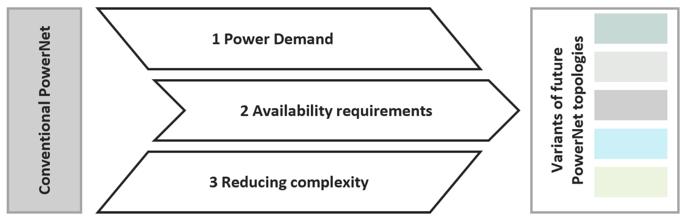
Figure 2.
(a) A simplified Matlabs Simulink / Simscape simulation model to investigate the influence of different power net parameters on transient behavior; (b) the main effects of the analyzed parameters on the resulting maximum voltage (); (c) selected two-factor interactions on maximum voltage and stabilization time (d). The load resistance in particular interacts strongly with the load capacitance and wire inductance in terms of the over-voltages that occur. For example, a high load resistance in combination with a high wire inductance can lead to a approx. 40 % higher over-voltage than with a low wire inductance, while almost the same over-voltage occurs with a low load resistance.
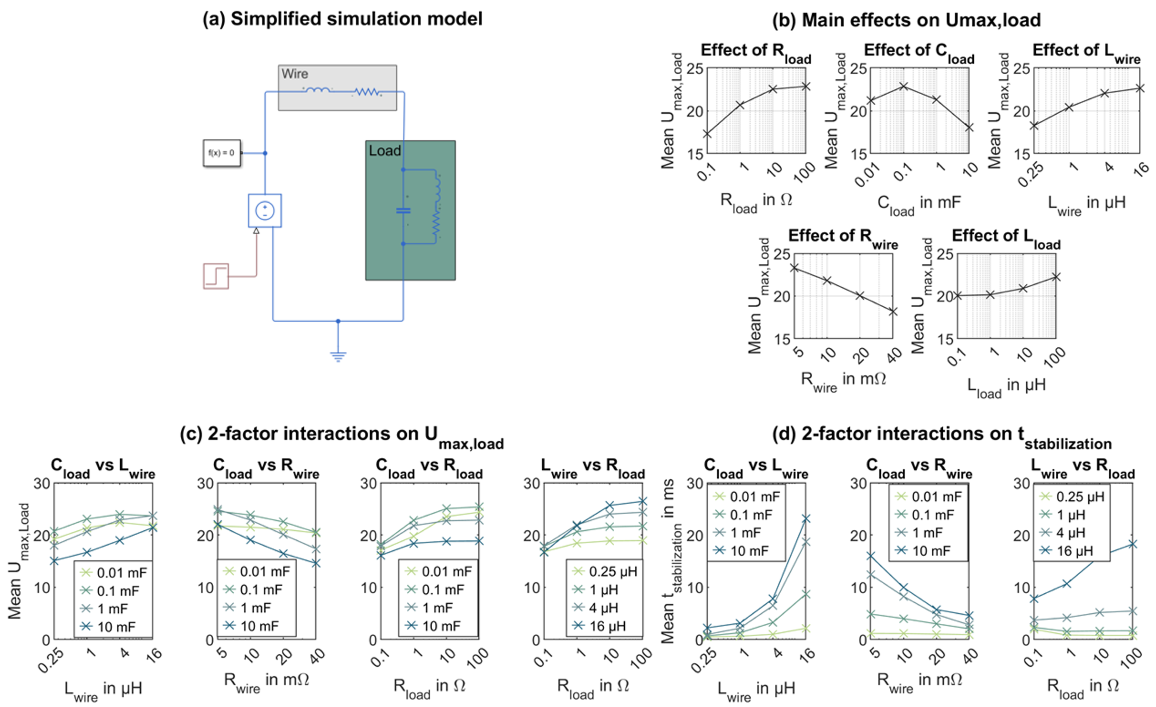
Figure 3.
(a)-(c): Setup for the different in-vehicle measurements; (d): fuse measurement adapters (red) and assembled measurement equipment consisting of fuse adapter (red) and LEM coil (blue); (e): Exemplary load profile measurement (electric window lifter) (f): Capacity measurement - Charge current.
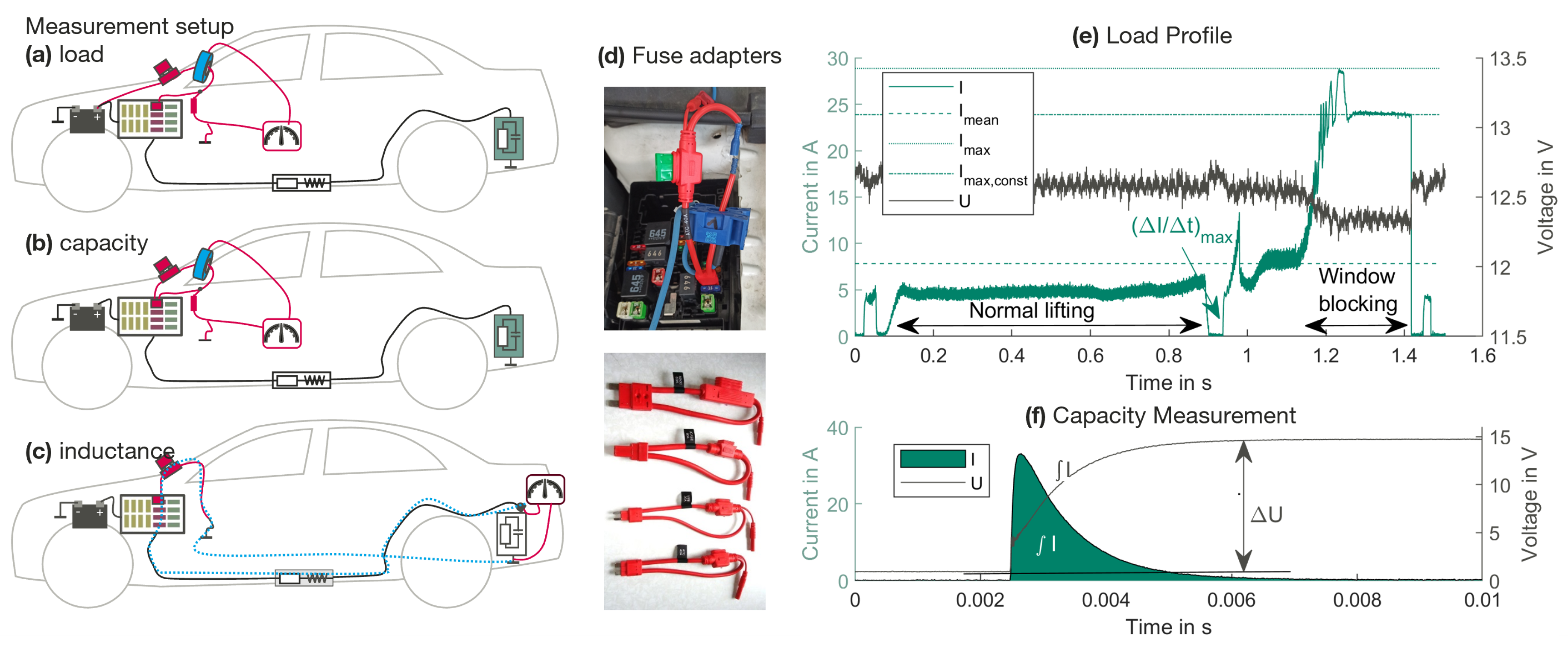
Figure 4.
Automotive wiring harness. (a) shows the typical routing and the fuse box positions for small and medium sized vehicles, (b) for large vehicles with dedicated BEV platform. (c) shows the 3D data which is used for the analyzes.
Figure 4.
Automotive wiring harness. (a) shows the typical routing and the fuse box positions for small and medium sized vehicles, (b) for large vehicles with dedicated BEV platform. (c) shows the 3D data which is used for the analyzes.
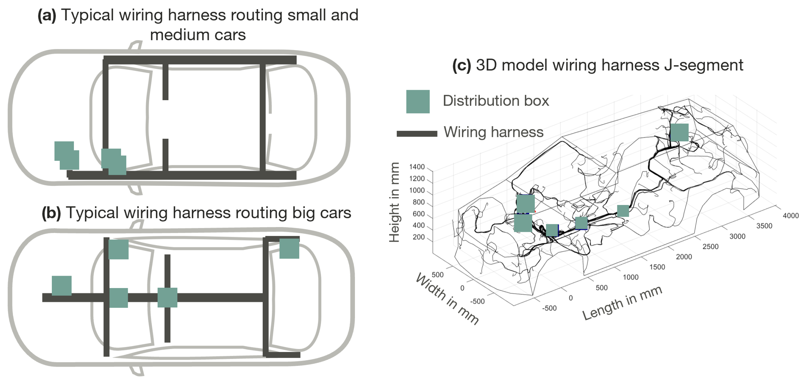
Figure 5.
Wiring harness analysis: (a) Length of the individual wires dependent on geometrical distance and vehicle segment, (b) wire length to wire length factor where the lines visualize the average and the filled circles represent loads within the engine compartment. A linear correlation between length factor and geometrical distance can be observed.
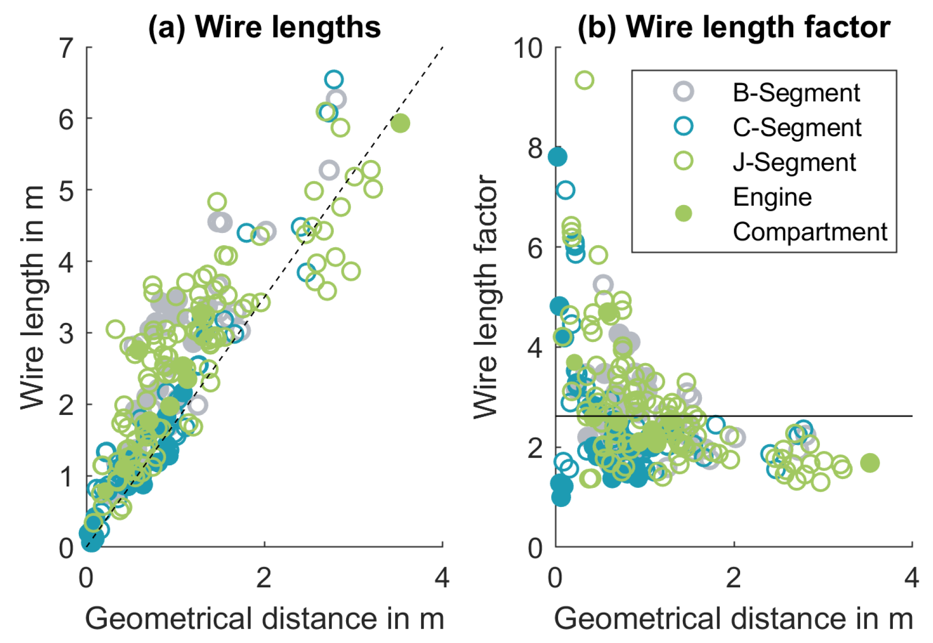
Figure 6.
Overview of the wiring harness length, cross-section resistance and inductance (B-Seg: black, C-Seg: red, J-Seg: green).
Figure 6.
Overview of the wiring harness length, cross-section resistance and inductance (B-Seg: black, C-Seg: red, J-Seg: green).
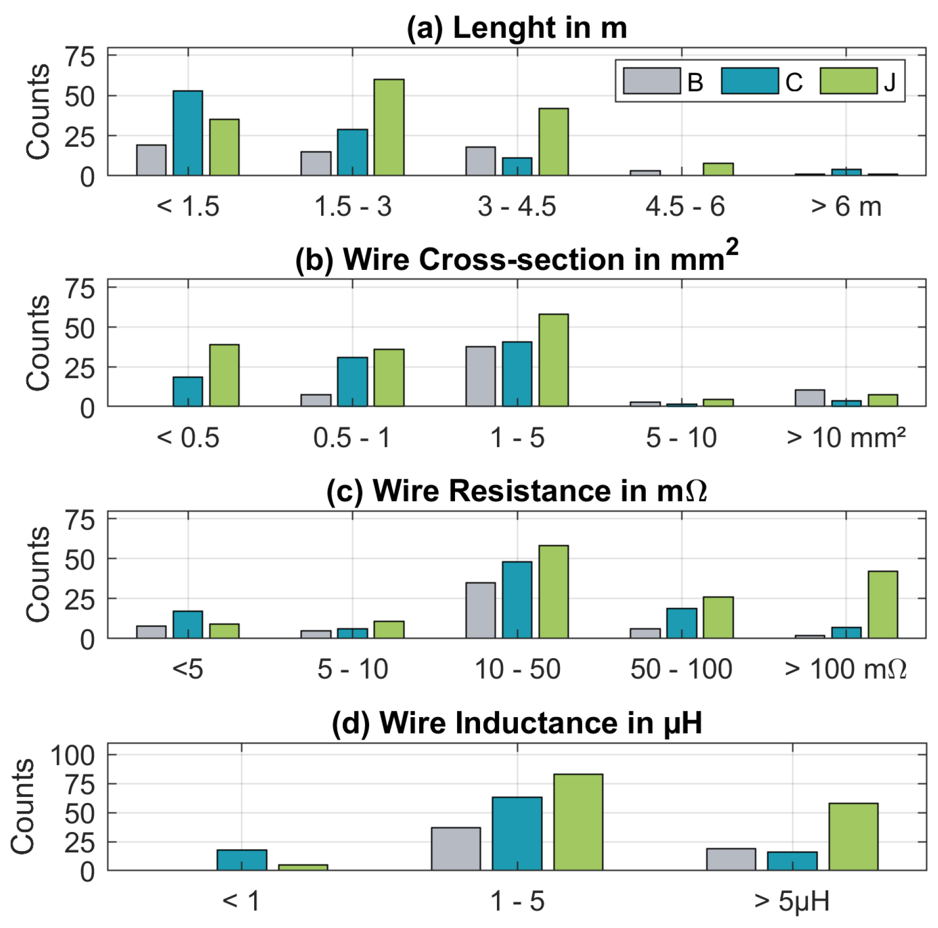
Figure 7.
(a)-(f): Comparison of installed 12 V loads in the analyzed vehicles. (g)-(i): Overview of the appearing maximum currents , the maximum constant currents and the capacities C. The counts indicate the number of corresponding loads. Only few loads require higher currents for a longer period of time.
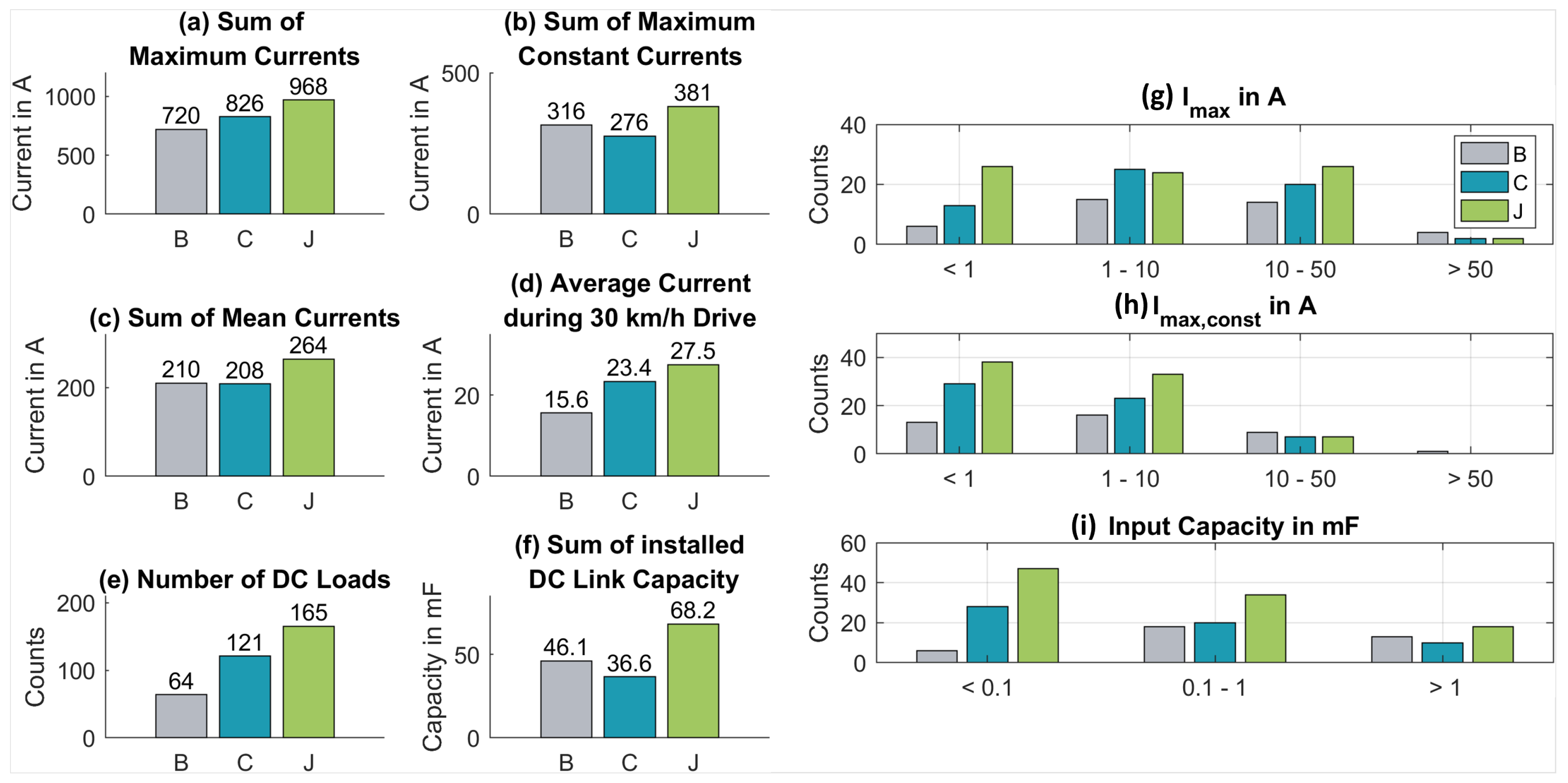
Figure 8.
Estimated series resistance of the input capacitors ESR*. As might be expected, the value decreases with increasing capacity.
Figure 8.
Estimated series resistance of the input capacitors ESR*. As might be expected, the value decreases with increasing capacity.
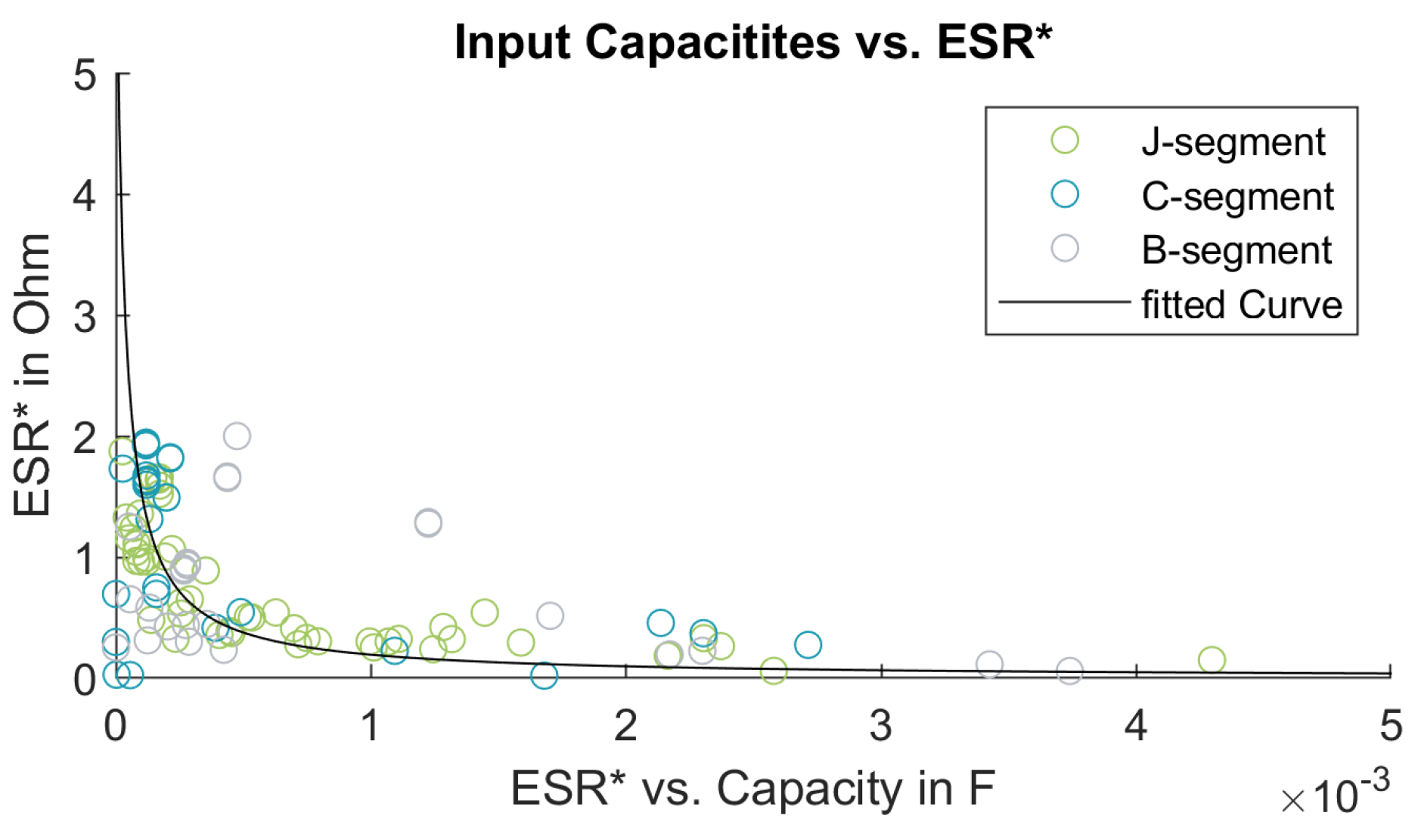
Figure 9.
3D positions of the loads distributed over the J-segment-vehicle. The circle color indicates the input capacitance and the line color of the wires shows the appearing maximum constant current (For reasons of clarity, capacities below 100 µH are shown in grey).
Figure 9.
3D positions of the loads distributed over the J-segment-vehicle. The circle color indicates the input capacitance and the line color of the wires shows the appearing maximum constant current (For reasons of clarity, capacities below 100 µH are shown in grey).
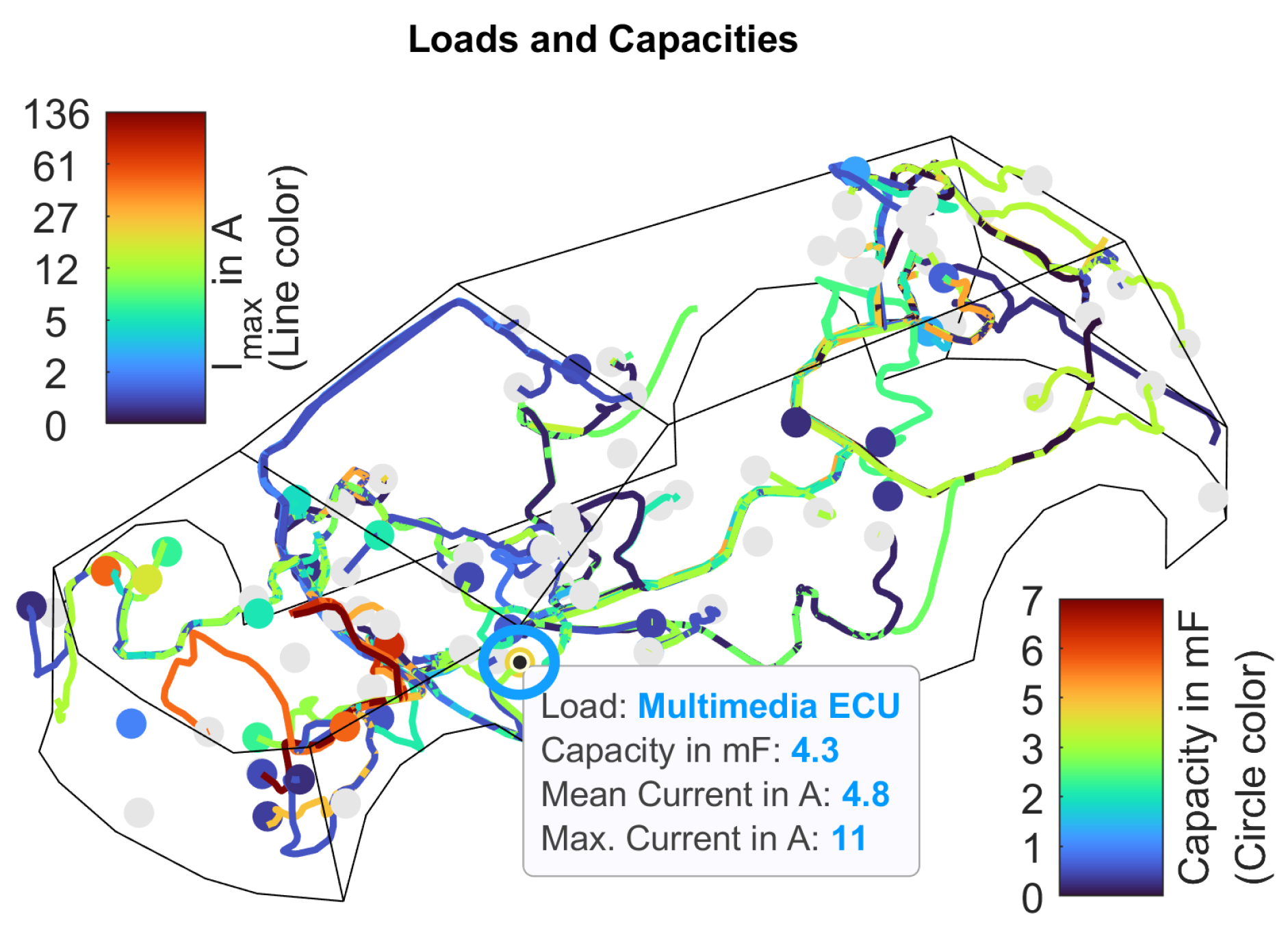
Figure 10.
2D map of capacities (a) and maximum constant currents (b) of the different vehicles. ’x’ indicates the position of the front lights, ’y’ the steering motor, and, ’z’ the braking system, high currents and capacities are concentrated in the front of the vehicle
Figure 10.
2D map of capacities (a) and maximum constant currents (b) of the different vehicles. ’x’ indicates the position of the front lights, ’y’ the steering motor, and, ’z’ the braking system, high currents and capacities are concentrated in the front of the vehicle
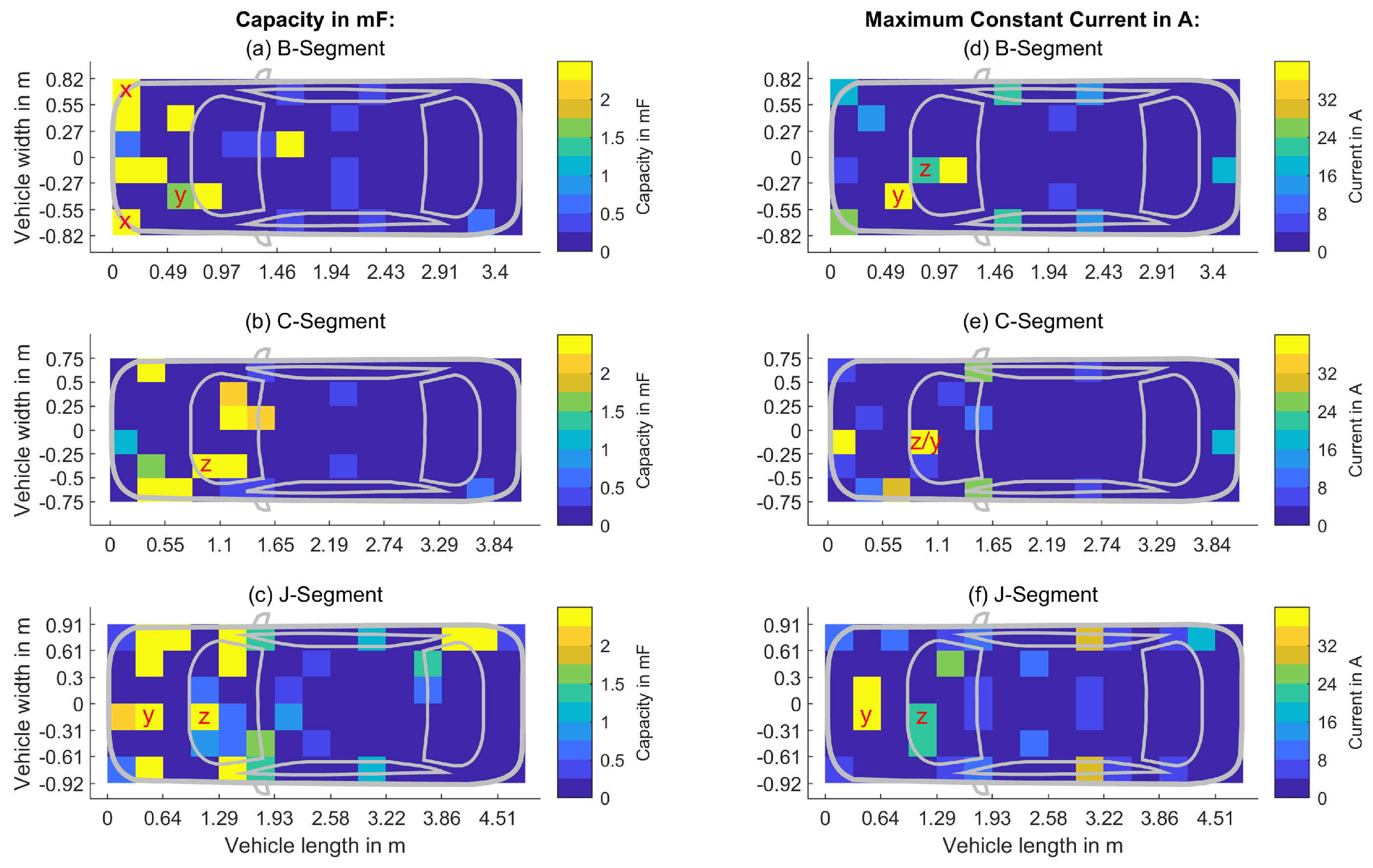
Figure 11.
Validation of the inductance: In average, the self-inductance calculated according to Equation 3 is closer to the measured values than the 1 µH/m value. The red boxes mark the wires with the same length, where the wires with the smaller cross-sections each have a higher inductance. The stars on top of the green bars mark the laboratory measurements.
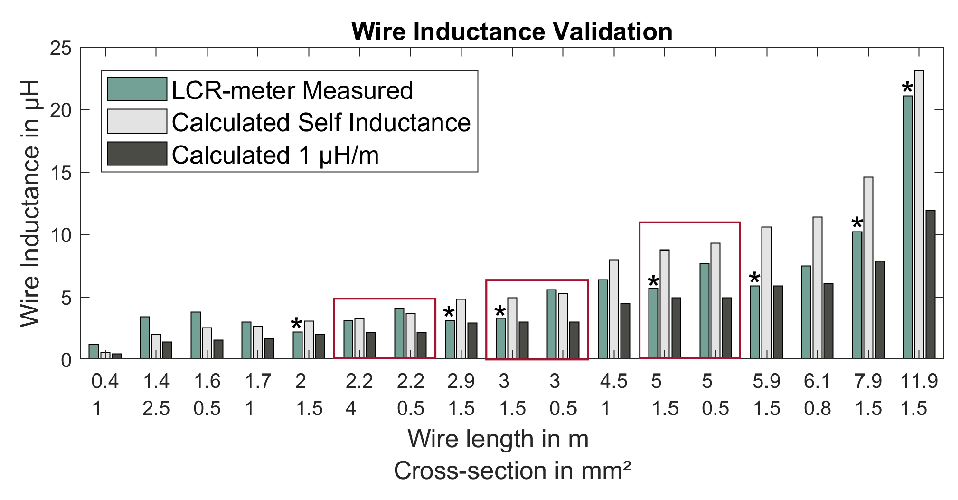

Table 1.
Calculated values for the mean voltage drop in the load wires, the ohmic losses in the overall wiring harness, the energy stored in the parasitic wiring harness inductances and the energy stored in the input capacities. The data is based on the measurements.
Table 1.
Calculated values for the mean voltage drop in the load wires, the ohmic losses in the overall wiring harness, the energy stored in the parasitic wiring harness inductances and the energy stored in the input capacities. The data is based on the measurements.
| B-segment | C-segment | J-segment | |
|---|---|---|---|
| in mV | 77 | 40 | 47.5 |
| in W | 202 | 167 | 173 |
| in J | 0.2 | 0.19 | 0.28 |
| in J | 9 | 7.5 | 14 |
Table 2.
Load data based on the measurements for the B / C / J segment. Only representative loads with and are shown. As can be seen many are associated with special equipment and thus only available in the more luxurious J-segment-vehicle. Literature values are provided on the right side of table [16,17].
| Load name | Fuse | I_max | I_max,const | I_mean | DI/dt | C | I_max (Literature) |
I_mean (Literature) |
|---|---|---|---|---|---|---|---|---|
| ADAS ECU | - / - / 10 | - / - / 4 | - / - / 4 | - / - / 3 | - / - / 4 | - / - / 2,2 | ||
| Brake | 120 / 163 / 100 | 111 / 100 / 80 | 18 / 14 / 17 | 18 / 14 / 17 | 14 / 38 / 79 | 0,1 / 2,9 / 7,2 | ||
| Cabin Fan | 40 / 30 / - | 26 / 8 / - | 23 / 5 / - | 18 / 3 / - | 3 / 3 / - | - / 2 / - | 12-29 | 7-29 |
| Cabin heater | 100 / - / - | 75 / - / - | 50 / - / - | 40 / - / - | 44 / - / - | 0 / - / - | 107-286 | 71-214 |
| Climate system | 10 / 8 / - | 1 / 2 / - | 0 / 1 / - | 0 / 1 / - | 0 / 2 / - | 1,2 / 1,5 / - | ||
| Display | - / 8 / 10 | - / 2 / 2 | - / 1 / 1 | - / 0 / 1 | - / 1 / 1 | - / 2,1 / 1,2 | ||
| Door lock | - / - / 20 | - / - / 8 | - / - / 7 | - / - / 6 | - / - / 6 | - / - / - | ||
| Electric tailgate | - / - / 40 | - / - / 32 | - / - / 8 | - / - / 4 | - / - / 5 | - / - / - | 7 | 2 |
| Electric window | 30 / 30 / 30 | 22 / 26 / 29 | 20 / 25 / 24 | 8 / 6 / 8 | 13 / 13 / 5 | 0,3 / - / - | 11 | 6-11 |
| Engine Fan | 60 / 50 / 125 | 8 / 47 / 47 | 5 / 40 / 40 | 3 / 33 / 33 | 3 / 7 / 7 | 3,4 / 0 / - | 57 | 14 |
| Front window heater | 0 / 40 / - | 0 / 30 / - | 0 / 29 / - | 0 / 28 / - | 0 / 29 / - | 0 / - / - | 9-143 | 18 |
| Light | 10 / 0 / 0 | 11 / 12 / 4 | 1 / 3 / 3 | 0 / 3 / 2 | 0 / 0 / 2 | 5,4 / 5,4 / 5,4 | 4 | 0-4 |
| Panel Heating | - / - / 30 | - / - / 11 | - / - / 6 | - / - / 4 | - / - / 6 | - / - / 0,1 | ||
| Panorma roof | - / - / 10 | - / - / 1 | - / - / 0 | - / - / 0 | - / - / 1 | - / - / 1,4 | ||
| Radar | - / - / 15 | - / - / - | - / - / - | - / - / - | - / - / - | - / - / 1,1 | ||
| Rear window heater | 40 / 30 / - | 22 / 17 / - | 19 / 16 / - | 17 / 14 / - | 22 / 17 / - | - / - / - | 9-14 | 9-14 |
| Seat heater | 30 / - / 30 | 6 / - / 12 | 6 / - / 7 | 5 / - / 3 | 3 / - / 7 | 0,4 / - / - | 14 | 2-14 |
| Steering | 80 / 80 / 250 | 67 / 98 / 136 | 56 / 31 / 32 | 16 / 31 / 32 | 31 / 12 / 9 | 1,7 / 0 / 0,5 | 107 | 29-57 |
| Trailer ECU | - / - / 20 | - / - / - | - / - / - | - / - / - | - / - / - | - / - / 5 | ||
| Trunk Lock | - / - / 40 | - / - / 7 | - / - / 6 | - / - / 4 | - / - / 2 | - / - / - | ||
| Washer pump | 20 / 0 / 30 | 15 / 15 / 25 | 5 / 5 / 6 | 6 / 6 / 6 | 14 / 14 / 24 | - / 0 / 0,4 | 7 | 4 |
| Water pump | - / 0 / 30 | - / 0 / 10 | - / 0 / 9 | - / 0 / 5 | - / 0 / 13 | - / 0 / 2,6 | 36 | 0-7 |
| Wiper back | 0 / - / 0 | 0 / - / 0 | 0 / - / 0 | 0 / - / 0 | 0 / - / 0 | 0 / - / 0 | ||
| Wiper front | - / 30 / 30 | - / 18 / 29 | - / 6 / 23 | - / 6 / 6 | - / 0 / 11 | - / 0,8 / 0,7 | 6-11 | 2-11 |
Disclaimer/Publisher’s Note: The statements, opinions and data contained in all publications are solely those of the individual author(s) and contributor(s) and not of MDPI and/or the editor(s). MDPI and/or the editor(s) disclaim responsibility for any injury to people or property resulting from any ideas, methods, instructions or products referred to in the content. |
© 2025 by the authors. Licensee MDPI, Basel, Switzerland. This article is an open access article distributed under the terms and conditions of the Creative Commons Attribution (CC BY) license (http://creativecommons.org/licenses/by/4.0/).
Copyright: This open access article is published under a Creative Commons CC BY 4.0 license, which permit the free download, distribution, and reuse, provided that the author and preprint are cited in any reuse.


