
Submitted:
23 March 2025
Posted:
24 March 2025
You are already at the latest version
Abstract
The present work deals with the fracture mechanics of crystalline rocks and in particular with the barrier integrity for the isolation of hazardous waste. The experimental data base is derived from the GREAT cell, a rock mechanics facility at the University of Edinburgh. The GREAT cell is a unique experimental facility that allows the investigation of thermo-hydro-mechanical (THM) processes in fractured rocks in rotating stress fields. The main idea of this work is to define a systematic benchmark suite for the development and testing of hydro-mechanical (HM) fracture mechanics codes based on GREAT cell experiments. The benchmarks represent simplifications of the original experiments to facilitate code testing. Two numerical fracture mechanics methods were used to simulate the complete benchmark suite, namely the variational phase field (VPF) and the lower-order interface element (LIE) methods. The numerical methods as well as Jupyter notebooks for pre- and post-processing are available in the open-source platform OpenGeoSys, following the FAIR principles of open science. This work is part of the DECOVALEX 2027 project, an international project to validate models and codes against experimental data.
Keywords:
Fracture mechanics
; Hydro-mechanical processes
; Variational phase field
; Lower-order interface elements
; GREAT cell
; DECOVALEX
; OpenGeoSys
1. Introduction
DECOVALEX is a long-standing international benchmarking project focusing on the systematic improvement of models for repository research [1,2,3,4,5]. Multi-physical/chemical processes, so-called thermo-hydro-mechanical-chemical (THMC) processes, which can be used to describe the temporal and spatial development of repository systems in terms of continuum mechanics, play a special role here. Because of the international participation, different host rocks have been addressed. Aside from clay and salt rocks, crystalline rocks have also been investigated [6,7,8] and are the focus of the present study. Benchmarking based on analytical solutions and/or code comparisons with academic, synthetic test examples has been broadly used to check the accuracy of numerical models and/or to test the correct implementation of numerical methods [9]. For DECOVALEX tasks, geotechnical experiments from underground laboratories are systematically selected to validate the numerical models using measured data. The transferability of the models from laboratory to in-situ scale plays a central role (experimental analysis) [10,11,12,13,14,15]. By validation, we mean the demonstration of physical adequacy of a model for a well-specified intent or context. This can be assessed via the ability of models to predict measurement results that were not used for model calibration (blind prediction, class A prediction). In recent DECOVALEX projects, tasks for the characterisation of repository systems in a geological context have also been defined and processed (performance assessment) [16]. The analysis of complete repository systems requires coping with the enormous computational effort. Therefore, methods of efficient computing (i.e. parallel computing) are becoming increasingly important for comprehensive safety analysis. Alternatively, methods are also being developed to find suitable surrogate models for the complex coupled THMC processes, using machine learning methods [17,18,19,20].
Despite the long tradition of DECOVALEX, the SAFENET Task brought fracture mechanics into the project for the first time in a systematic benchmarking during DECOVALEX 2023 [21]. Initially, model comparisons were carried out with defined analytical solutions [22], and mechanical (M), hydro-mechanical (HM) and thermo-mechanical (TM) experiments were carried out in the rock laboratories of the TU Bergakademie Freiberg [23], the University of Edinburgh [24,25,26] and KICT [27,28,29], respectively. In the present work, new test examples for fully coupled HM models will be developed on the basis of the GREAT (Geo-Reservoir Experimental Analogue Technology) cell laboratory experiments, which will be used for the experimental planning of corresponding experiments in the new DECOVALEX project 2027 (SAFENET 2).
The GREAT cell of the University of Edinburgh is a unique experimental facility for conducting triaxial test in a rotational stress field. This setup allows the measurement of fracture permeabilities under varying stress conditions. However, the complexity of this equipment makes it challenging to reproduce its results numerically. To overcome this, we developed a simplified benchmark version suited for numerical modeling. For the first time, numerical benchmarks will be proactively designed based on simplified examples derived from GREAT cell experiments (with laboratory replication planned for future work). This novel approach is addressing the ongoing challenge of accurately modeling fracture mechanics processes under varying pore pressures and mechanical loads (HM conditions).
Numerical modeling fracture mechanics under varying HM conditions is challenging, requiring precise numerical methods to replicate fracture behaviors observed in experiments like the GREAT cell. Numerical methods for fracture modeling are broadly classified into sharp and smeared fracture approaches [30]. Sharp fracture methods, such as the Extended Finite Element Method (XFEM) [31], Embedded Discontinuity Method [32,33,34], and Finite Element Method with universal meshes [35,36,37], explicitly represent fractures as discrete discontinuities. In contrast, smeared fracture methods, including Continuum Damage Mechanics [38], Gradient Damage Mechanics [39], and the phase-field method [40], model fractures as distributed regions integrated into a continuum framework using concepts of non-locality [41].
In the current research, two numerical methods are adopted to explore fracture behavior in porous media under conditions relevant to GREAT cell benchmarks: the Variational Phase-Field (VPF) method [40,42] and lower-dimensional interface elements (LIE) [43]. The VPF method provides a robust framework for simulating fracture nucleation, propagation, and branching under hydro-mechanical coupling. In contrast, the LIE approach explicitly represents fracture surfaces and their hydro-mechanical interactions using lower-dimensional elements. Together, these methods offer a comprehensive understanding of fracture processes in coupled hydro-mechanical systems within porous materials. Both approaches are implemented within the finite element framework of OpenGeoSys [44,45].
The paper is structured as follows. A brief description of the methodology, including the experimental concept of the GREAT cell experiments and the theoretical basis for the variational phase field (VPF-FEM) and lower-order interface element (LIE-FEM) methods, which represent two different approaches to fracture mechanics, is briefly summarised in Section 2.2. The benchmarking procedure is presented in Section 3, starting with the concept and parameter settings (Section 3.1). The results obtained by both the VPF-FEM and LIE-FEM methods for intact and fractured rock samples are presented in detail in the following subsections 3.2, 3.3. Fracture propagation is discussed in Section 3.4. In the discussion, Section 4, the results of the VPF-FEM and LIE-FEM methods are compared with respect to effective permeability, fracture width, and breakdown pressure. The conclusions, Section 5, summarise the main results of the present work and give an outlook on future work. Moreover, the present work contributes to digitisation and open science in THM modelling [46] by providing a set of Jupyter notebooks for documentation and reproducibility of the presented benchmarks (see Appendix and Supplementary Material).
2. Methodology
2.1. Experimental concept
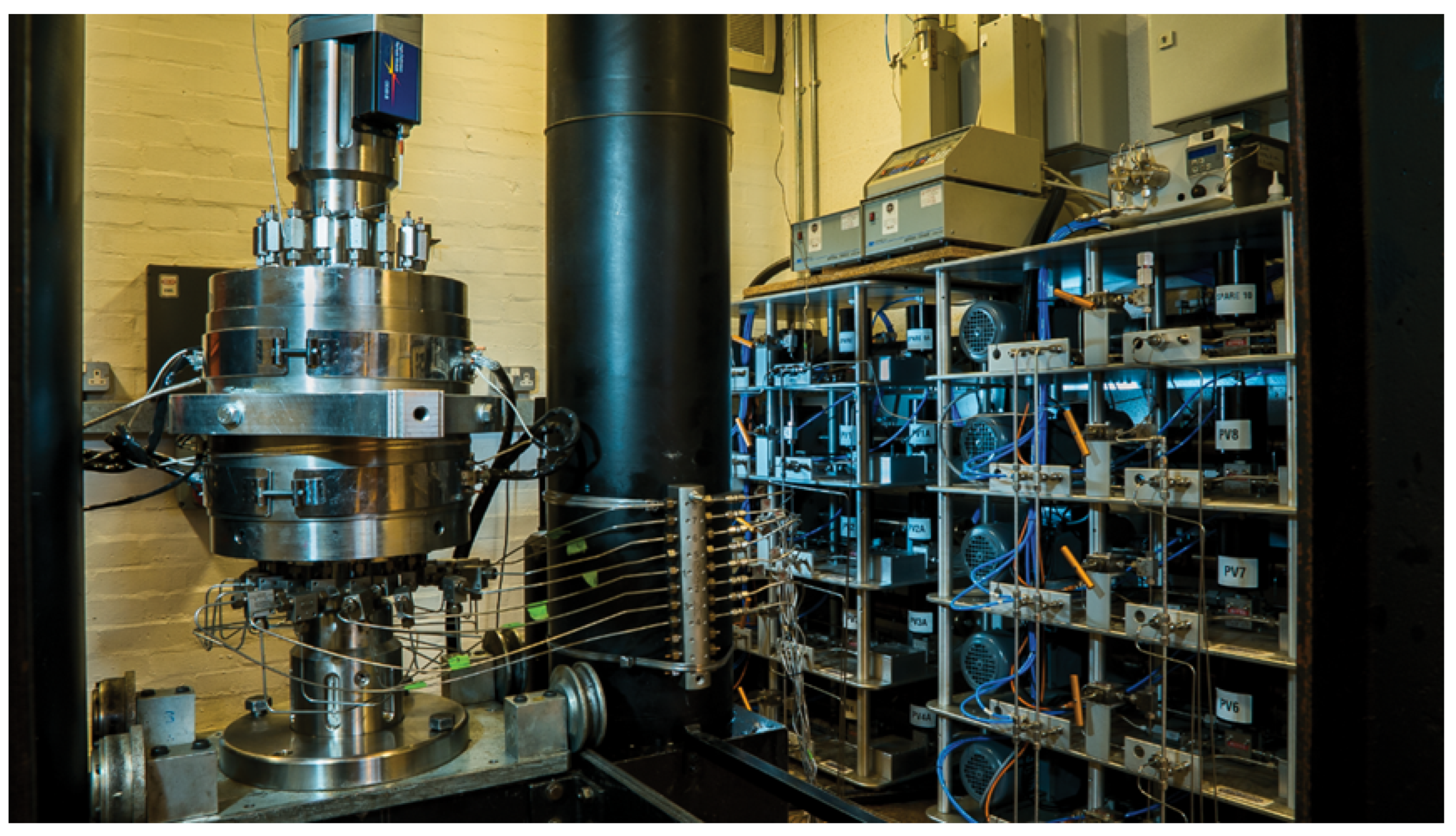
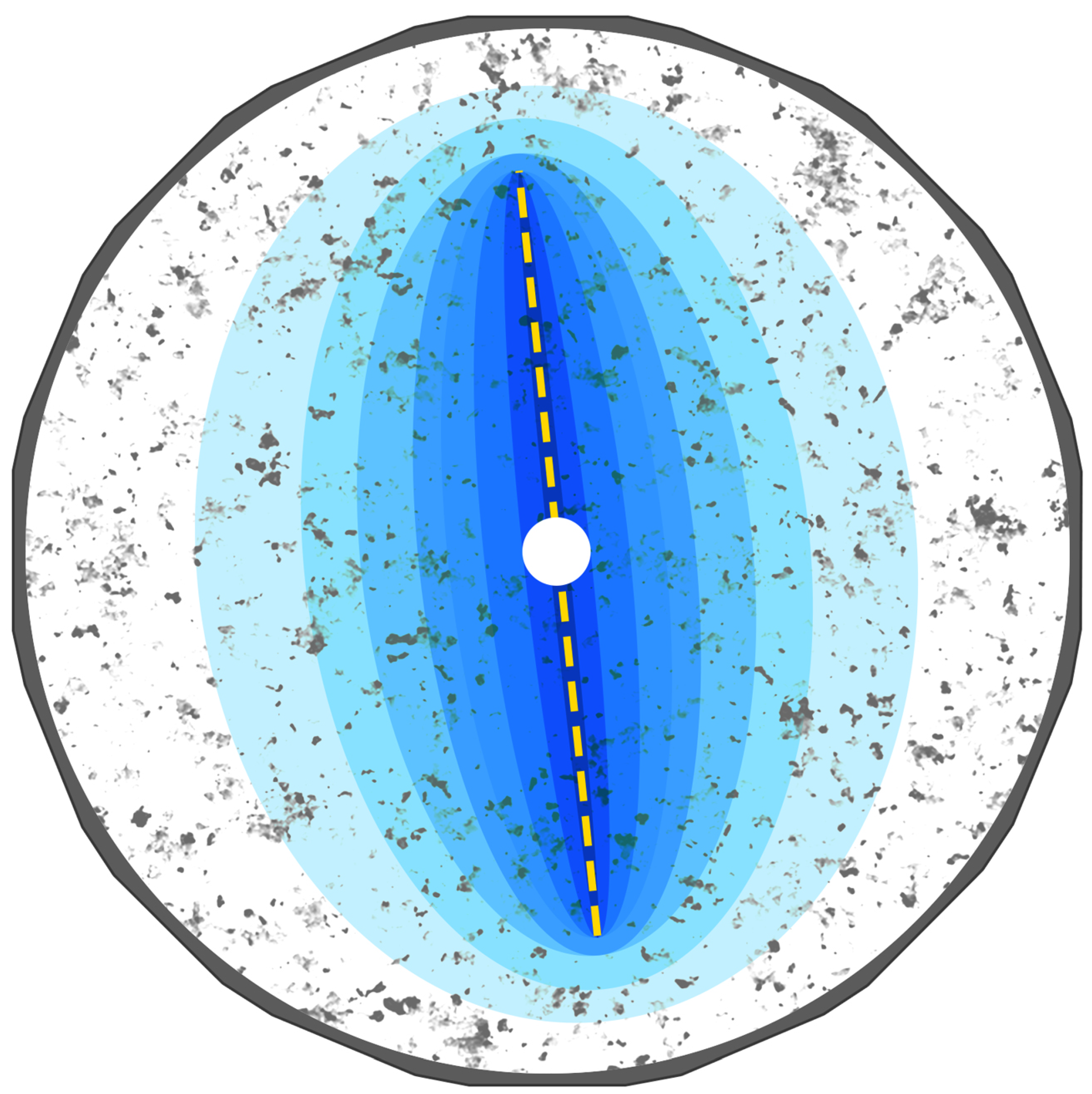
The GREAT cell, depicted in Figure 2, is designed to reproduce subsurface conditions in the laboratory down to a depth of 3.5 km in terms of geomechanical stress and geothermal reservoir conditions on 200 mm diameter rock samples containing fracture networks, thereby enabling these predictions to be validated. The cell represents a major new development in experimental technology, uniquely creating a truly poly-axial rotating stress field, facilitating fluid flow through the samples, and using state-of-the-art fibre-optic strain sensing for high-resolution circumferential strain measurements combined with fluid pressure, capable of thousands of detailed measurements per hour. The GREAT cell will help to better understand and predict fracture propagation and subsequent fluid flow characteristics, which is critical for geo-energy technologies that exploit favourable geological conditions to store or extract fluids from the subsurface. It is well known that fracture permeability decreases non-linearly with increasing normal stress, but the relationship between shear displacement and fracture permeability is less well understood [24,26].
Figure 1.
(a) Typical rock sample and (b) simplification for benchmarking of GREAT cell.
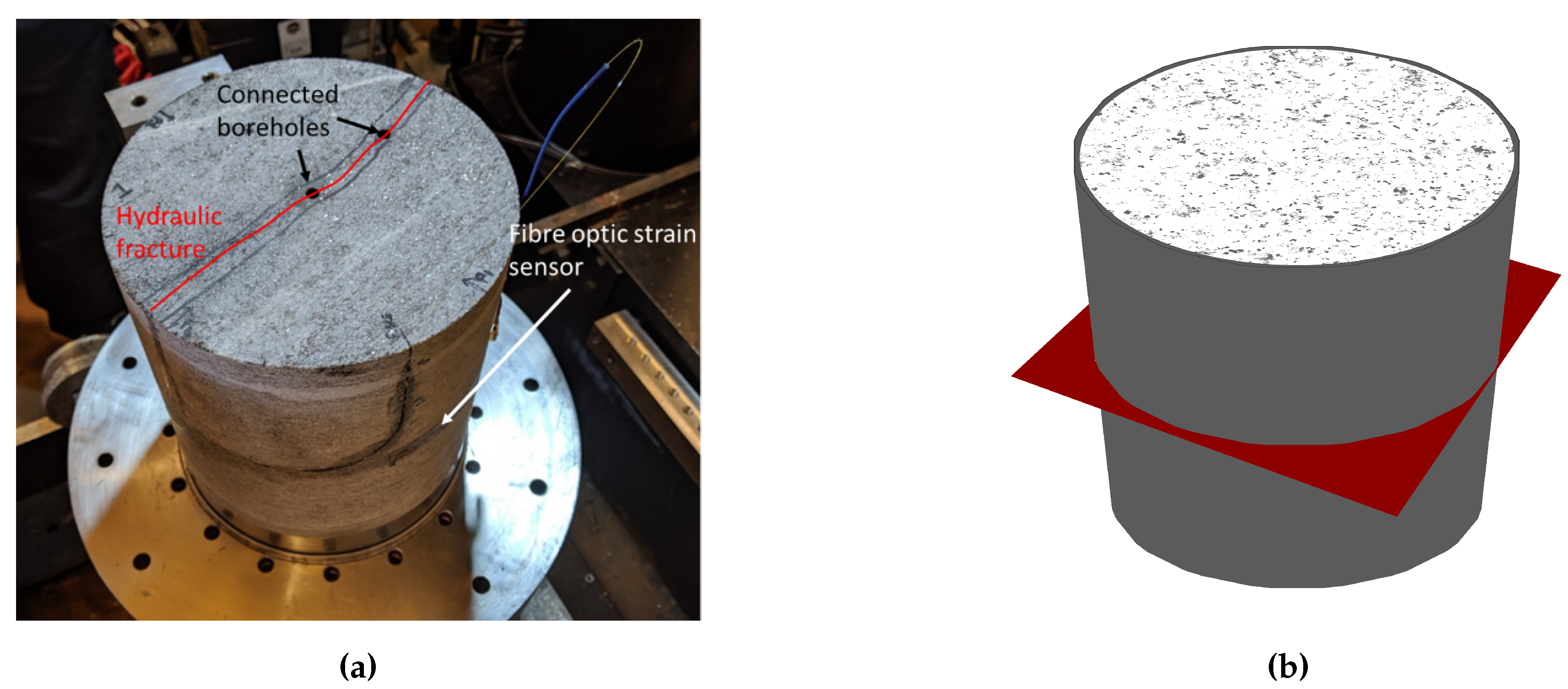
Figure 2.
The GREAT cell facility.
In [21], we compared numerical results with experimental data of GREAT cell. However, fracture mechanics under coupled conditions in a novel experimental facility pose challenges for accurate numerical reproduction. This study does not include experimental comparisons; instead, it focuses on developing a benchmark suite tailored for researchers, particularly within the DECOVLEX project. This suite can serve model comparison in a setting that closely resembles GREAT cell tests and can help design tests to be performed specifically for model calibration and validation.
2.2. Mathematical models
The theory of linear poro-elasticity proposed by Biot [47] is widely used to model the deformation of fluid-saturated porous media with a nearly-incompressible fluid (i.e., a fluid with constant density and a finite bulk modulus).Under quasi-static conditions, the governing equations for poro-elastic deformation and fluid flow in porous media and fractures are:
where is the density of the porous medium, given by , where represents the porosity. is the fluid density, and is the solid density; p is the pore pressure, and is the Biot coefficient. and are the bulk moduli of the solid matrix and a nearly-incompressible fluid, respectively. is the permeability tensor, and is the dynamic viscosity; w is the fracture aperture. and are source terms for the matrix and fracture, respectively, while represents the leak-off term. represents the gradient operator along the fracture plane, and is a Dirac delta function supported on the fracture surface.
The poro-elastic stress definition, based on Biot theory [47], is given by , where is the total stress, is the effective stress, and is the identity tensor. The constitutive relation for poro-elastic materials describes the incremental relationship between stress and strain as , where and represent incremental changes in effective stress and linearized strain, respectively, and is the fourth-order elasticity tensor. The linearized strain tensor is defined as , which expresses strain in terms of the displacement gradient while ensuring symmetry.
Section 2.2 combines mass conservation and Darcy’s law for fluid flow in the matrix (porous medium). Section 2.2 addresses mass conservation in fractures using the lubrication approximation. Boundary conditions for these equations involve specifying displacements or tractions, and pressures or fluxes on the relevant boundaries and fracture interfaces.
2.2.1. Variational Phase Field Approach
The variational phase-field method is widely used in computational fracture mechanics because it effectively models fracturing across different media. Its applications are brittle fracture [48,49,50,51,52,53], ductile fractures [54,55], fatigue failure [56,57], creep-induced fractures [58], dynamic fracture [59,60,61], desiccation cracks [62,63], CO2/hydraulic fracturing [64,65,66], fractured reactive porous media [67,68], grain size effects [69], nuclear waste repositories [70,71], and fractography [72,73], among others. Its versatility and robustness make it a valuable tool for fracture propagation analysis.
Grounded in Griffith’s fracture criterion [74], the variational phase-field approach effectively addresses its inherent limitations, particularly the dependence on high stress singularities for crack initiation. Francfort and Marigo [42] redefined Griffith’s criterion by minimizing total energy, combining strain and fracture surface energy:
This model overcomes the original criterion’s limitations, enabling fracture propagation modeling without known paths and handling nucleation and branching. However, numerically implementing crack surface energy for complex geometries is challenging due to the evolving discrete crack set .
To overcome this, Bourdin et al. [49] proposed a variational phase-field model with a scalar phase-field variable and a regularization length parameter . The regularized total energy is:
with the model (, ) and the model (, ) [50]. is the degraded strain energy (see the Appendix H for various strain energy decompositions); For brevity, we denote the strain tensor simply as .
To extend the formulation to hydro-mechanical fracturing, one can decompose the strain energy of a porous medium based on Biot’s work [75] as follows:
the first term represents the strain energy of the dry, fractured medium (dry), modeled using phase-field methods. The second term accounts for poro-elastic coupling in a saturated, fractured medium (wet), with . Here, (Biot modulus) measures fluid-saturated material compressibility.
Recent studies [76,77,78] show that varies in presence of fracture and in phase-field models, the drained bulk modulus degrades as , where . You and Yoshioka [65] proposed that Biot coefficients depend on the phase field and splitting strain energy approaches. Therefore, the Biot coefficients are expressed as functions of v and the strain tensor :
To model fluid flow in fractured porous media, considering both the matrix and fractures, the phase field variable plays a key role in adjusting the permeability tensor. Accordingly, we introduce an anisotropic permeability tensor defined as:
where, represents the intrinsic permeability of the matrix, adjusts the impact of fractures on permeability, w denotes the fracture aperture following the cubic law, and denotes the normal vector to the fracture plane. By approximating the displacement jump vector in terms of the maximum principal strain and a characteristic length scale , we derive:
in this approach, we adopt a concept similar to that proposed by You and Yoshioka [65], while the normal vector is defined based on the principal strain direction. This definition provides greater robustness near the fracture tip and avoids the challenges associated with using , resulting in a simpler and more effective solution for our model.
The ?? and Section 2.2 for hydro-mechanical fracturing using a variational phase field approach are summarized as follows:
here, represents the phase-dependent Biot coefficient; denotes the phase field-dependent permeability tensor, Equation (5); p is the pressure, and the continuity of pressure across fractures ensures , where and are fracture pressure and matrix pressure, respectively. Additionally, Effective stress depends not only on displacement but also on the phase field variable v. Since the fluid is incompressible, Equation (8) is divided by to obtain a formulation based on volumetric fluxes (compare Section 2.2).
2.2.2. Lower-dimensional interface elements
The lower-dimensional interface element approach is specifically designed for pre-existing fractures and fracture paths within the framework of the FEM [43]. This technique represents fractures using lower-order elements and incorporates a partial modification of the Extended Finite Element Method (XFEM) [31].
One of its key features is the local enrichment of the finite element approximation space of displacement, allowing for discontinuities across fractures. This is mathematically expressed as
where denotes the FE displacement approximation at point , is the displacement jump, N stands for the shape function, the global enrichment function, I is the set of nodes in the domain, and is a subset of all nodes in the lower order interfaces.
In addition to displacement enrichment, the method accounts for stress within fractures by employing a localized constitutive law. For elastic deformation, this relationship is defined as
where is the stiffness tensor whose coefficient matrix in the fracture’s natural coordinate system reads
with and are the joint shear and normal stiffness, respectively. and govern the coupling effects between normal and shear displacements.
The governing equations for hydro-mechanical processes in fractured porous media involve a coupled system that accounts for both momentum balance and mass conservation within the porous matrix and the the fracture interface . The momentum balance equation, incorporating the enriched finite element approximation of displacement, is given by:
Mass conservation in the porous matrix and the fracture follows:
Here, is the specific storage, where fluid compressibility, , is considered in the storage term, while the fluid density is assumed to be constant, following a nearly-incompressible formulation; and represent the intrinsic permeabilities of the fracture and matrix, respectively. The terms and describe fluid exchange between the fracture and the surrounding matrix. Both mass balance equations are normalized by the fluid density .
3. Numerical Benchmarks
3.1. Concept
A comprehensive benchmarking exercise is performed to establish the models’ capabilities and required settings, such as the required discretization for comparable accuracy. These benchmarks are simplified versions of the GREAT cell experiments, focusing on general features like fracture patterns, rotating boundary conditions, and coupled processes. These benchmark exercises are conducted in 2D (plane strain), representing a horizontal section through the middle of the rock samples tested in the GREAT cell (Figure 1b). This 2D plane-strain approach allows the main characteristics of hydro-mechanical (HM) fracture mechanics to be studied efficiently. The benchmarking concept involves a stepwise increase in complexity, including both mechanical (M) and hydro-mechanical (HM) approaches.
We distinguish two main types of benchmarks: intact and fractured rock tests (Figure 3a). In the first type, an intact rock sample is subjected to rotating external stress conditions () and fluid is injected from a central borehole ():
- : Intact rock sample under rotating boundary conditions.
- : Intact rock sample with fluid injection.
For the fractured rock samples, two subtypes are also considered: static and propagating fractures. Static fractures are studied as full (, ) and half-fractured (, ) versions to have a symmetric and non-symmetric case. Again, mechanical and hydro-mechanical versions are studied, the latter with fluid injection into the rock fracture:
- : Fully fractured sample.
- : Half-fractured sample.
- : Fully fractured sample with inflow-outflow.
- : Half-fractured sample with inflow-outflow.
Finally, fracture propagation conditions are studied by injecting fluid into a pre-existing fracture () and fracture nucleation from borehole ():
- : Propagation of pre-existing fracture by fluid injection.
- : Fracture nucleation from borehole by fluid injection.
We repeated each of these benchmarks under different loading conditions and material properties. The material properties are provided in Table 1, and the fluid properties are listed in Table 2. The computational model incorporates two distinct elastic materials within its domain: a central circle ( m) of rock surrounded by a rubber sheath in a 2D configuration.
The boundary conditions applied in the simulation include both Dirichlet and Neumann conditions. For the momentum balance equation in the sample domain, Dirichlet boundary conditions are used to fix displacement at specific points and prevent rigid body rotation by enforcing zero displacement at selected locations. Mathematically, these conditions are defined as:
where and are the displacement components in the x and y directions, respectively. Neumann boundary conditions define the normal stress on the Pressure-Exerting Elements (PEE’s) and Dynamic-Sealing Strips (DSS’s).
A triaxial loading system is used to generate a sinusoidal response in the sample. To study the effect of poly-axial rotating loading, this load is rotated (e.g., Load A is rotated 45° clockwise to generate Load B). The loading specifications for the PEE’s are detailed in Table 3. The stress on the DSS’s,
is determined as the average of the stresses applied to the adjacent PEE’s. The arrangement of PEEs and DSSs is provided in Figure 3b.
3.2. Intact Rock Tests
3.2.1. Intact Rock Sample under Rotating Boundary Conditions–
The primary objective of the first benchmark exercise is to evaluate the mechanical deformation of different rock samples in the GREAT cell under various boundary conditions in a 2D plane strain setup. The benchmark considers a plane strain triaxial stress condition, where the in-plane principal stresses are defined as MPa and MPa. Meanwhile, the out-of-plane stress is governed by the plane strain constraint, given by, for both Greywacke and Gneiss samples.
Figure 5 presents the trace of effective stress () and volumetric strain versus angle for intact samples: (a) Greywacke and (b) Gneiss, using the VPF-FEM method as an example. Note that in Figure 5, the stress distribution is illustrated across the entire domain, while the distribution of volumetric strain is shown within the region m for the benchmarks. The strain in the PEE’s is relatively high due to their soft material properties, which is why the visualization of strain results is limited to the region near the core of the sample.
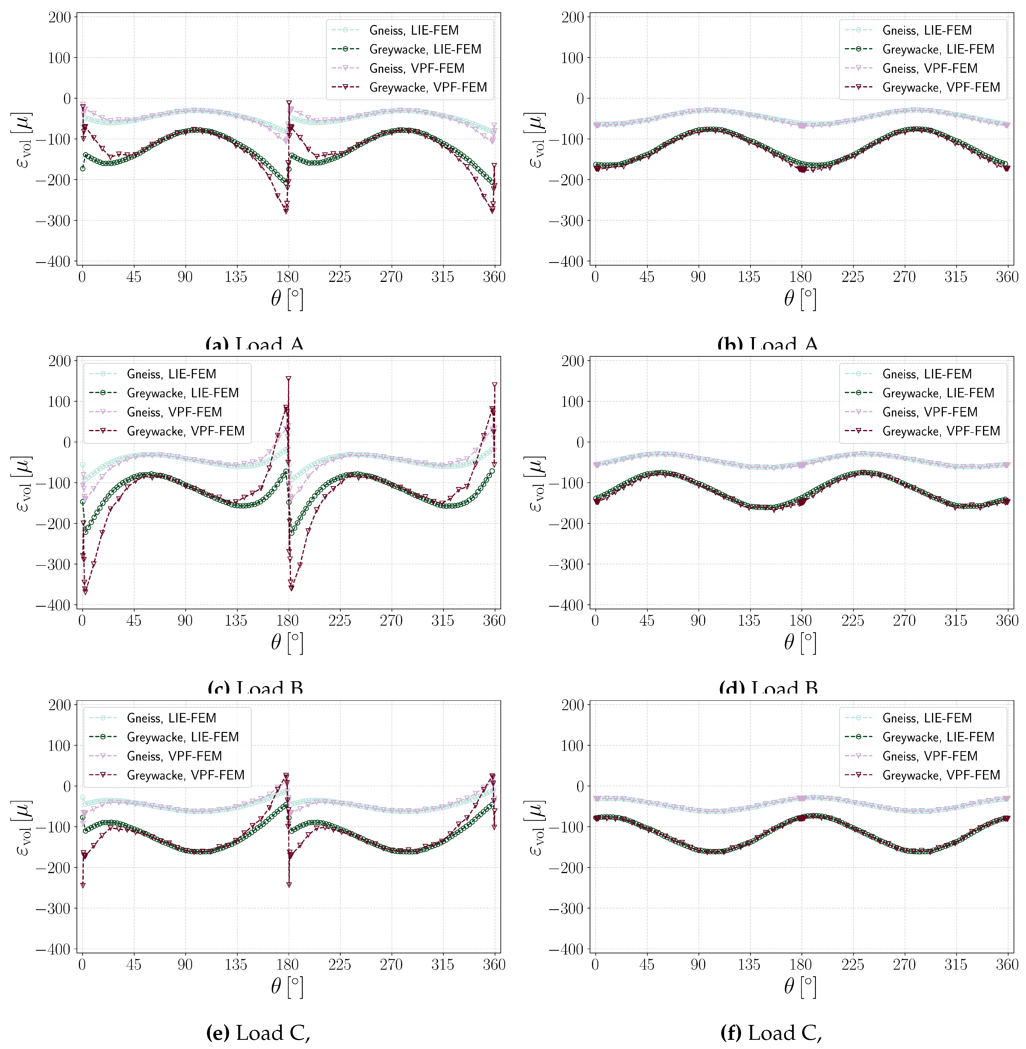
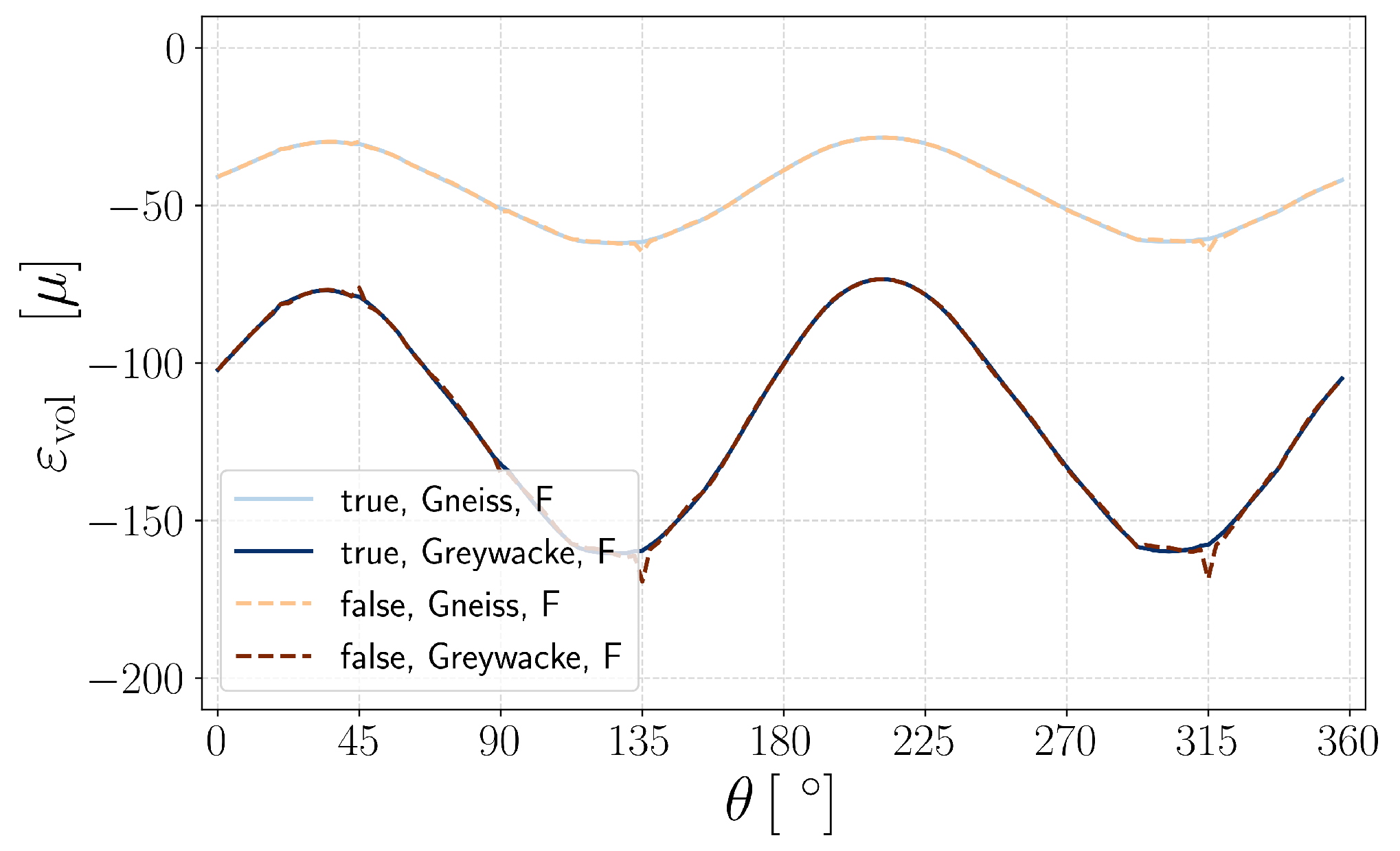
Figure 6a illustrates the volumetric strain versus angle for intact Greywacke and Gneiss samples subjected to triaxial loading conditions (Load A, see Table 1). The results indicate that VPF-FEM and LIE-FEM effectively replicate similar deformation responses, demonstrating strong agreement between the two methods for intact samples. Greywacke experiences greater negative volumetric strain compared to Gneiss under poly-axial loading because of its lower Young’s modulus and higher Poisson’s ratio, which contribute to increased bulk compressibility.
3.2.2. Intact Rock Sample with Fluid Injection–
This benchmark, which does not consider any fracture, is designed to verify the basic computational setting for hydro-mechanical simulations. In addition to the mechanical loads, a zero constant pore pressure is prescribed at the outer boundary. At the center of sample, fluid is injected at a rate of m3/s,
The hydro-mechanical simulations follows a two-stage process: a 3000 s equilibrium phase under mechanical loading to stabilize initial conditions, followed by a 500 s fluid injection phase to model fluid flow (see Section 4.1 for more details).
Figure 7 presents the pressure, trace of effective stress, and volumetric strain profiles of the Greywacke and Gneiss samples for the test under Load A at the final time (e.g. LIE-FEM). For the volumetric strain profile the results of m are again excluded. This benchmark highlights the hydro-mechanical contrast between Greywacke and Gneiss under fluid injection. Greywacke, with lower stiffness, higher permeability, and greater porosity, enables widespread strain, indicating higher bulk compressibility. In contrast, Gneiss, with higher stiffness, lower permeability, and lower porosity, experiences localized pressure buildup, higher stress concentration, and restricted strain, leading to lower compressibility.
Additionally, Figure 6b illustrates the volumetric strain at the probe-circle for different samples using both VPF-FEM and LIE-FEM. The results show that an increase in pressure at the center of the domain leads to a decrease in effective stress, resulting in a reduction in the magnitude of compressive volumetric strain compared to .
3.3. Fractured Rock Tests
3.3.1. Static Fracture Samples
In this section, numerical simulations are performed on static fracture samples using both VPF-FEM and LIE-FEM, comparing their results.
To simulate the effect of fracture orientation on strain without generating a new mesh for each case, the fracture is kept identical while the poly-axial loading is rotated. The material properties of the sample are listed in Table 1, and the PEE and DDS loads are detailed in Table 3.
Fully Fractured Sample–
In this benchmark, 2D plane strain numerical simulations are performed to establish a baseline model for assessing the impact of fracture orientation on strain distribution under poly-axial loading. A planar fracture within the specimen, , is considered, under poly-axial loading applied on PEE’s and DSS’s (Table 3).
Figure 8 illustrates the profiles of stress and volumetric strain for the Greywacke sample in the test subjected to Load B at the final time (LIE-FEM and VPF-FEM). As the Figure 8 indicates, the VPF-FEM results exhibit larger strain near fracture tip.
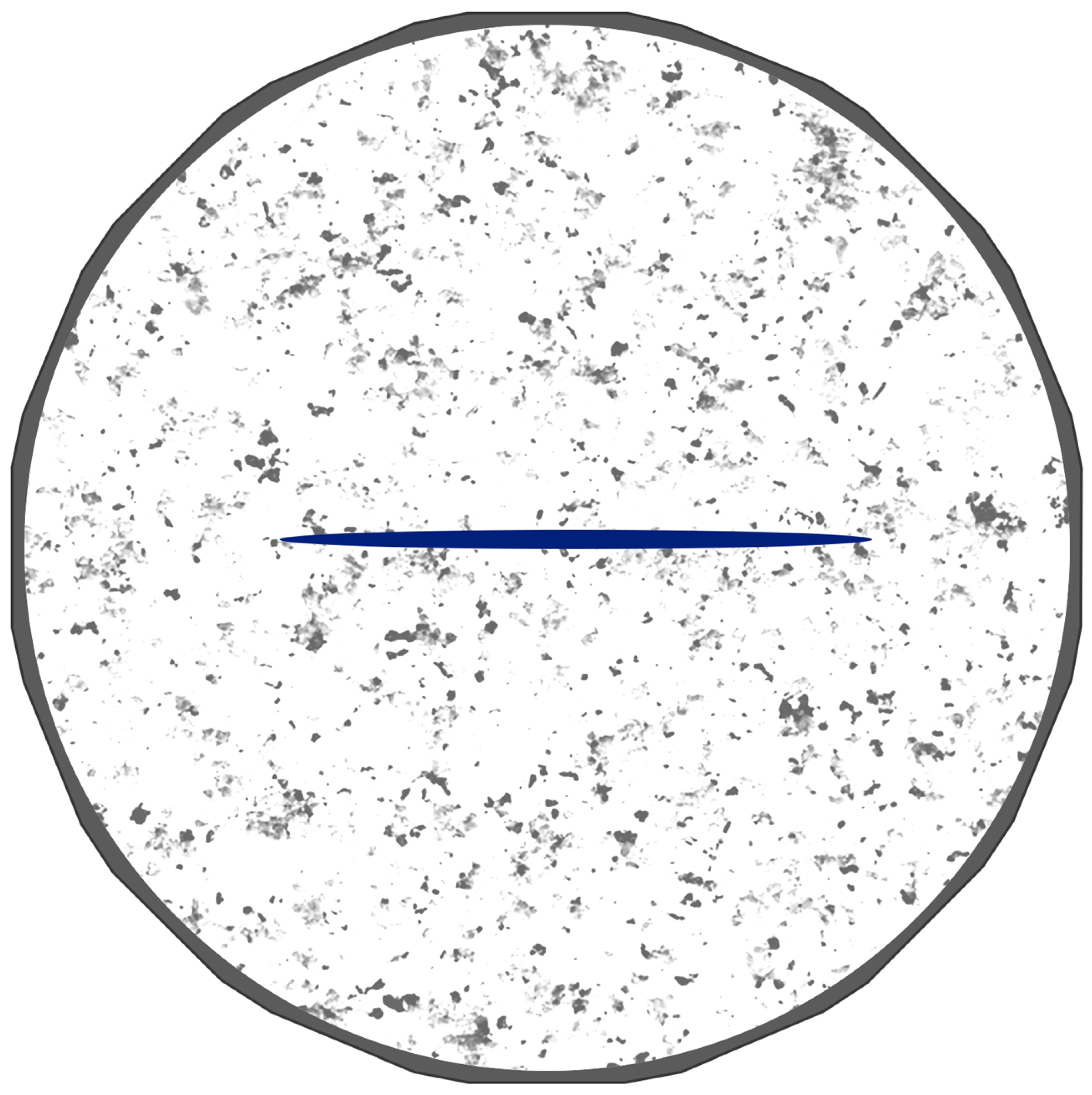
Figure 10a, Figure 10c, and Figure 10e illustrate the volumetric strain at the probe-circle for Greywacke and Gneiss samples under varying loading conditions. The spikes in the VPF-FEM and LIE-FEM curves indicate a jump in volumetric strain as the probe circle passes through the fracture locations.
The results demonstrate strong consistency away from the fracture. However, at the intersection of the probe-circle and the fracture, the VPE-FEM method shows a higher absolute value of volumetric strain. These differences arise from fundamental distinctions between the approaches. In the LIE-FEM model, both normal and shear fracture stiffness are explicitly accounted for, whereas in the VPF-FEM framework, fracture behavior under mixed loading is dictated by the chosen strain energy decomposition (see Appendix G). Here, the Volumetric–Deviatoric strain energy decomposition is adopted. A sensitivity analysis exploring the impact of different strain energy decompositions in VPF-FEM and fracture stiffness in LIE-FEM is provided in Section 4.2.
Half Fractured Sample–
In this section, all input data and boundary conditions provided in , except a single wing fracture, defined as , is considered.
Figure 9 illustrates the profiles for trace of stress and volumetric strain obtained from both the VPF-FEM and LIE-FEM methods under the test subjected to Load B at the final time . Both methods capture the stress singularity at the fracture tips.
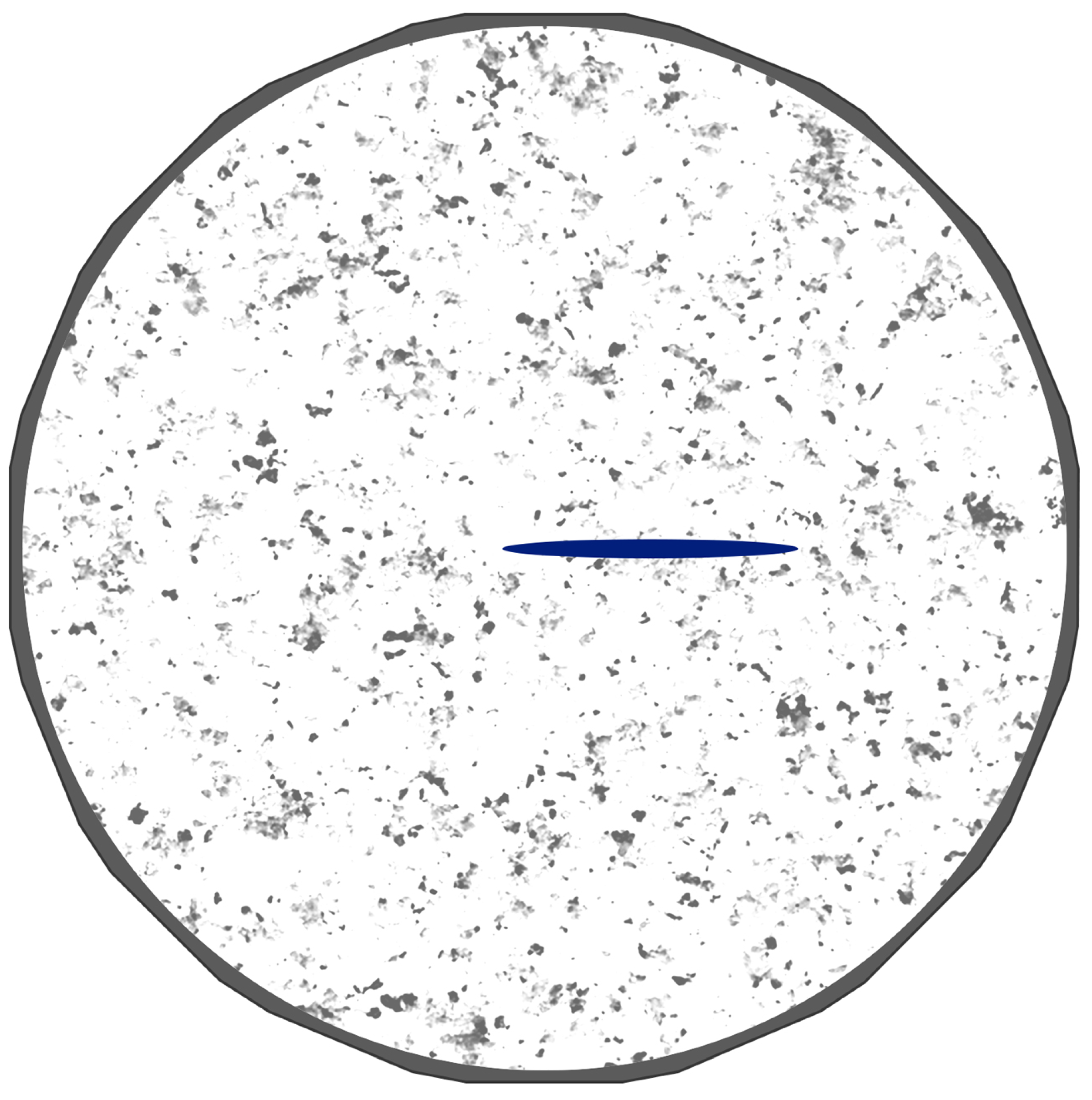
Figure 10b, Figure 10d, and Figure 10f compare the volumetric strain versus angles at the probe-circle for Greywacke and Gneiss samples under various loading conditions. The results demonstrate strong overall agreement, with differences between the two methods diminishing as the probe-circle moves farther from the fracture tip.
Figure 9.
: Trace of effective stress and volumetric strain profiles of the Greywacke sample for the test under Load B at the final time (LIE-FEM & VPF-FEM).
Figure 9.
: Trace of effective stress and volumetric strain profiles of the Greywacke sample for the test under Load B at the final time (LIE-FEM & VPF-FEM).
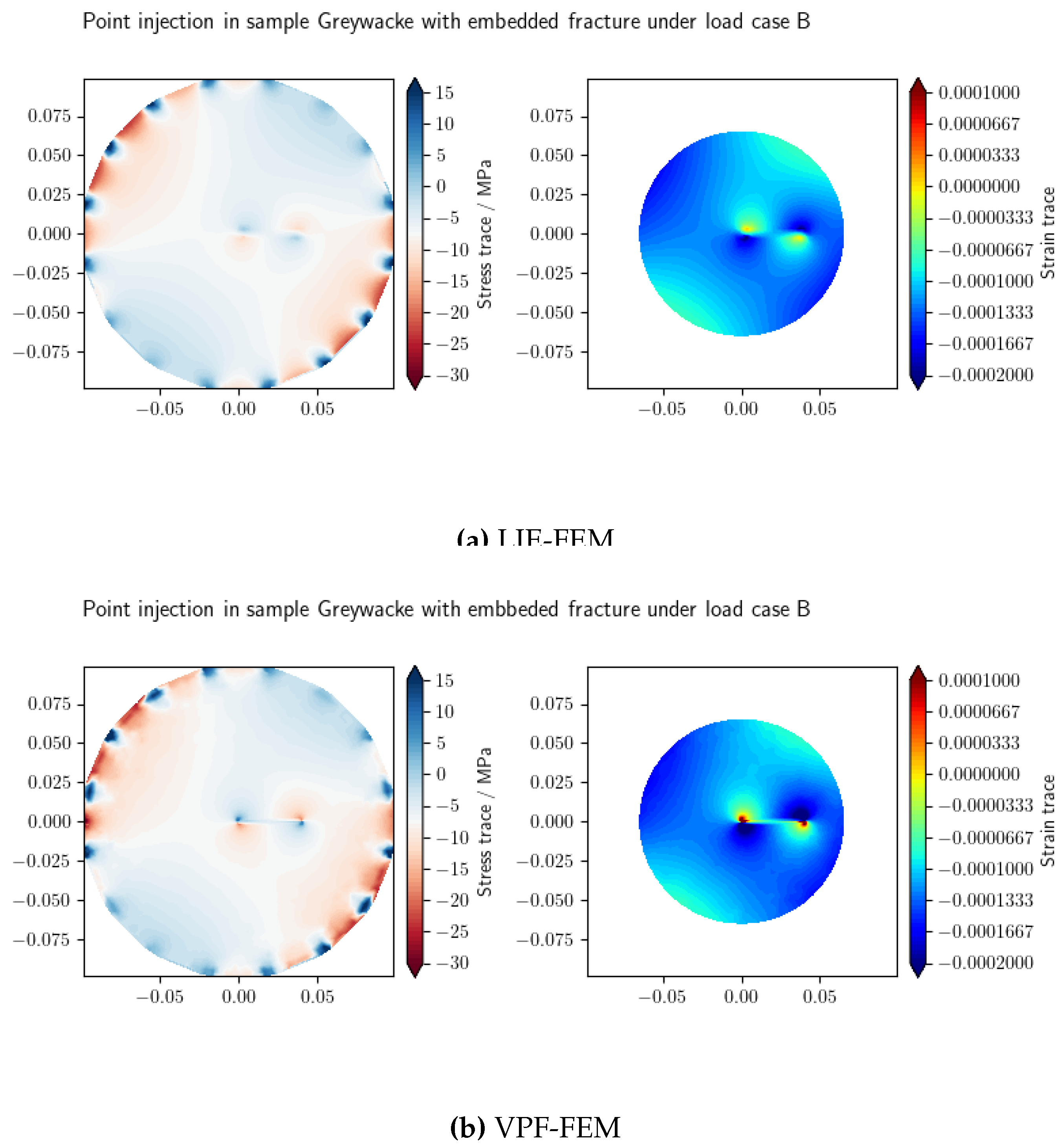
Figure 10.
/: Volumetric strain versus angle for fractured samples under different loading conditions as detailed in Table 3.
Figure 10.
/: Volumetric strain versus angle for fractured samples under different loading conditions as detailed in Table 3.
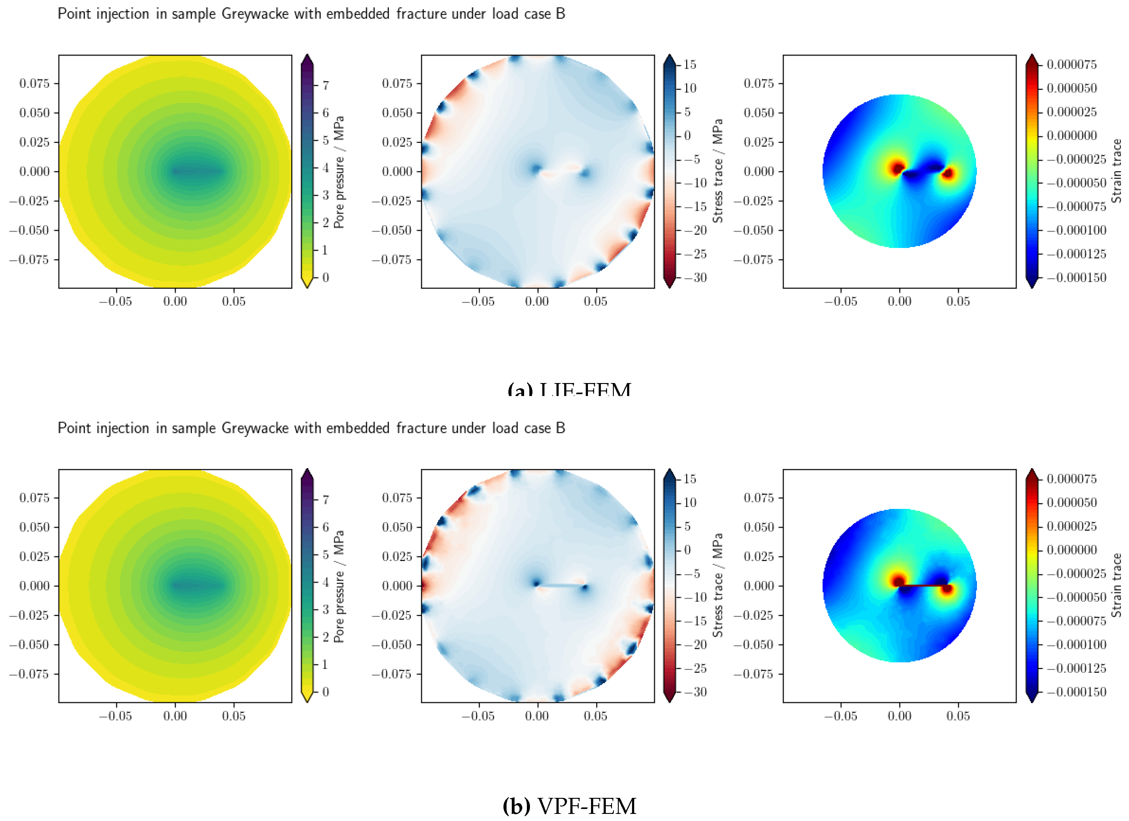
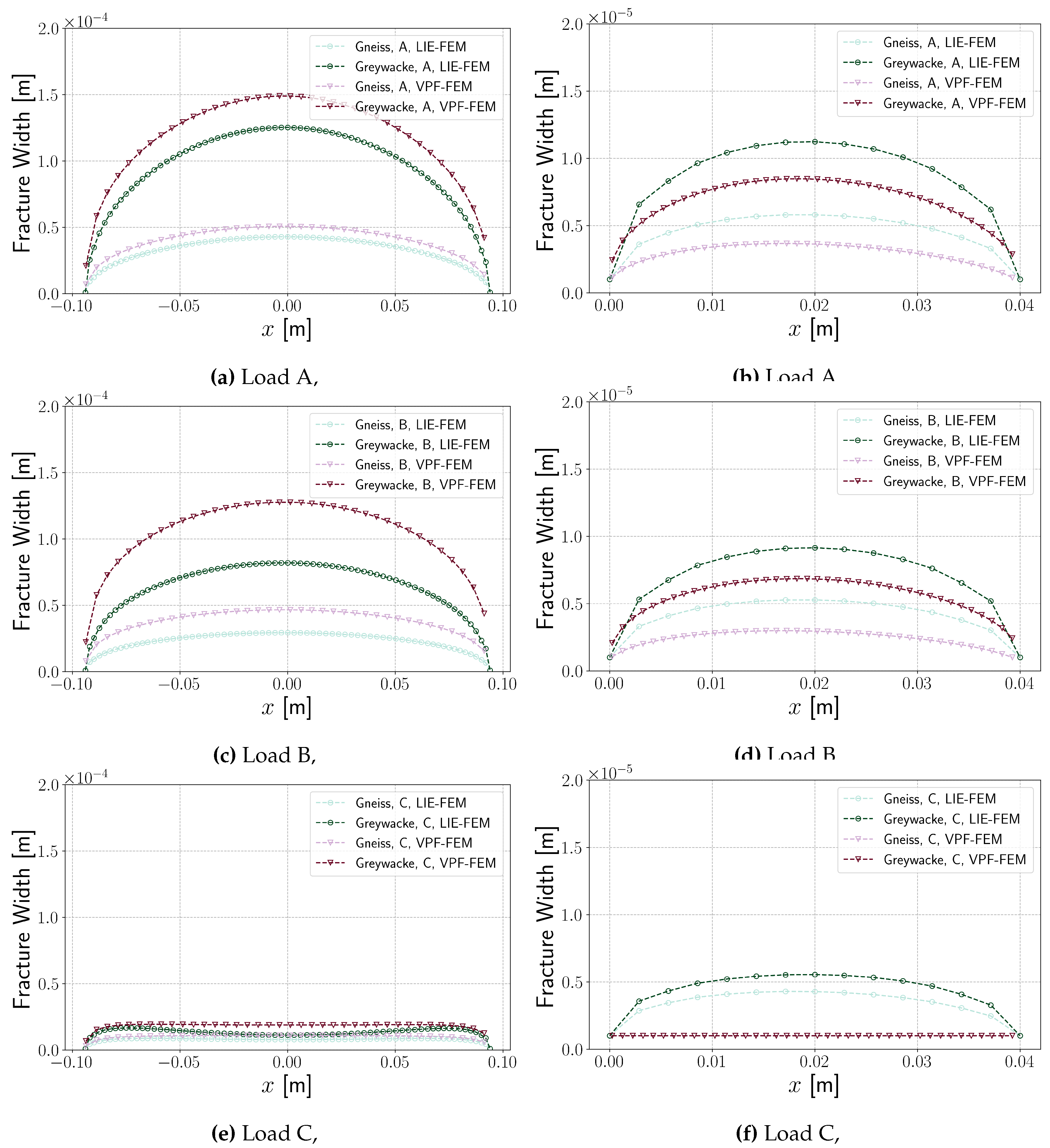
Fully Fractured Sample with Fluid Injection–
In order to explore how fracture permeability varies across different materials and different load conditions, a series of hydro-mechanical simulations () is performed. Five distinct load conditions (Table 3) are considered, each designed to create different angles between the second principal stress direction ( MPa) and the plane of PEE 5. A planar fracture within the specimen , is analyzed.
For the fluid flow, the initial pressure throughout the domain is set as MPa. Dirichlet boundary conditions are imposed such that MPa. After allowing the system to stabilize for 3000 s to reach equilibrium, fluid is injected at the center with an injection rate of (25 ml/min) for 500 s. Furthermore, the initial fracture width is considered to be m.
Figure 11 presents the pressure, effective stress trace, and volumetric strain profiles of the Greywacke sample from the test under Load B at the final time step (), using LIE-FEM and VPF-FEM. As illustrated in Figure 11b, the stress within the recaptured region diminishes to nearly zero. This phenomenon occurs due to the Isotropic model used in VPF-FEM for this benchmark. When the phase field variable v reaches zero, it leads to complete stress attenuation at the fracture.
Figure 13a, Figure 13c, and Figure 13e illustrate volumetric strain versus angle for fractured samples under different loading conditions, as detailed in Table 3 for . A jump is observed where the probe-circle intersects the fracture. This jump is more significant in the VPF-FEM method for hydro-mechanical fractures due to the higher strain values within the fracture captured by VPF-FEM.
Figure 14a, Figure 14c, and Figure 14e show the fracture width along the fracture for fractured samples under different loading conditions. The fracture width in all cases is of a similar order; however, differences arise due to variations in the numerical models. In VPF-FEM, the width is calculated using a strain-based method, whereas in the LIE-FEM method, it is explicitly determined from displacement.
Figure 12.
: Pressure, trace of effective stress, and volumetric strain profiles of the Greywacke sample for the test under Load B at the final time (LIE-FEM & VPF-FEM).
Figure 12.
: Pressure, trace of effective stress, and volumetric strain profiles of the Greywacke sample for the test under Load B at the final time (LIE-FEM & VPF-FEM).
Half Fractured Sample with Fluid Injection–
In this section, all input data and boundary conditions provided in are used. A single wing fracture, defined as , is considered. For the boundary conditions related to fluid flow, a Dirichlet boundary condition with a pressure of MPa is applied on the right side of the fracture. After allowing the system to stabilize for 3000 s to reach equilibrium, fluid is injected with an injection rate of (25 ml/min) on the left side of the fracture.
Figure 12 presents the pressure, stress trace, and volumetric strain profiles of the Graywacke sample from the test under Load B at the final time step (), using LIE-FEM and VPF-FEM.
Figure 13b, Figure 13d, and Figure 13f illustrate volumetric strain versus angle for fractured samples under different loading conditions, as detailed in Table 3 for . As shown, there is no jump in this set of figures since the probe-circle does not pass through the fracture.
Figure 14b, Figure 14d, and Figure 14f illustrate the fracture width along the fracture for fractured samples under different loading conditions. Figure 14f (Load C, VPF-FEM) shows that the fracture width remains nearly unchanged. The higher stress perpendicular to the fracture plane under Load C prevents opening, likely due to the Isotropic model used in VPF-FEM for this benchmark. In contrast, LIE-FEM shows clear fracture opening for Load C.
Figure 13.
/: Volumetric strain versus angle for fractured samples under different loading conditions as detailed in Table 3.
Figure 13.
/: Volumetric strain versus angle for fractured samples under different loading conditions as detailed in Table 3.
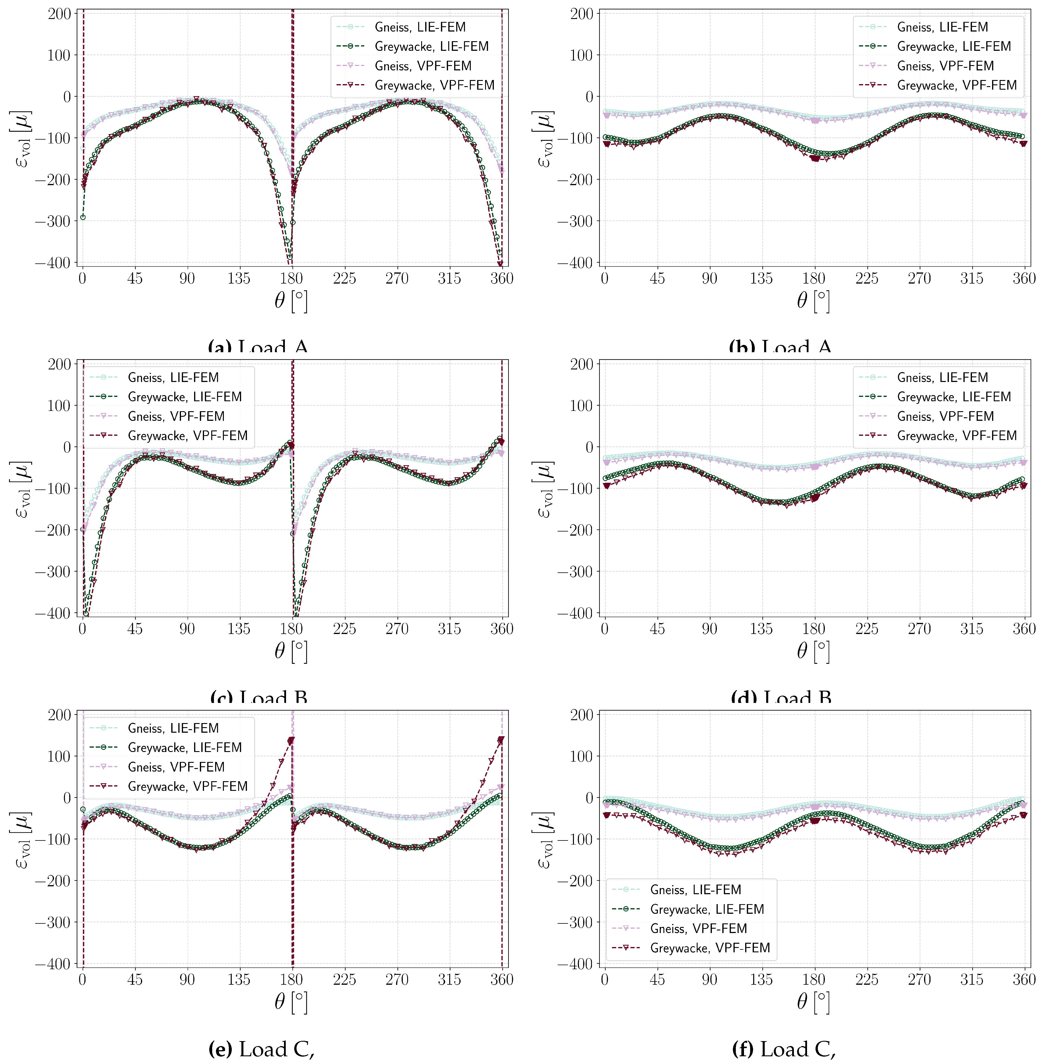
Figure 14.
/: Fracture width along the fracture for fractured samples under different loading conditions, as detailed in Table 3.
Figure 14.
/: Fracture width along the fracture for fractured samples under different loading conditions, as detailed in Table 3.
3.4. Fracture propagation
3.4.1. Hydraulic Fracturing (pre-existing fracture)–
In this set of benchmarks, hydraulic fracturing is simulated under various boundary conditions. Fluid is injected at the center of an inclined fracture to model the fracturing process. To evaluate the impact of poly-axial stress boundary conditions on fracture propagation, three load scenarios (A, B, and C in Table 3) are defined. A planar, initially inclined fracture, is considered. The initial fracture width is set to m with an initial pressure of 0.1 MPa. The radial stress is applied at the boundary ( Table 3), and it is allowed to equilibrate over 3000 s. Subsequently, an injection rate of m2/s is applied at a single line element ( m) at the center of the fracture. The rest of the material and fluid properties used in the simulations are presented in Table 1 and Table 2. Here, the Volumetric-Deviatoric strain energy decomposition is used.
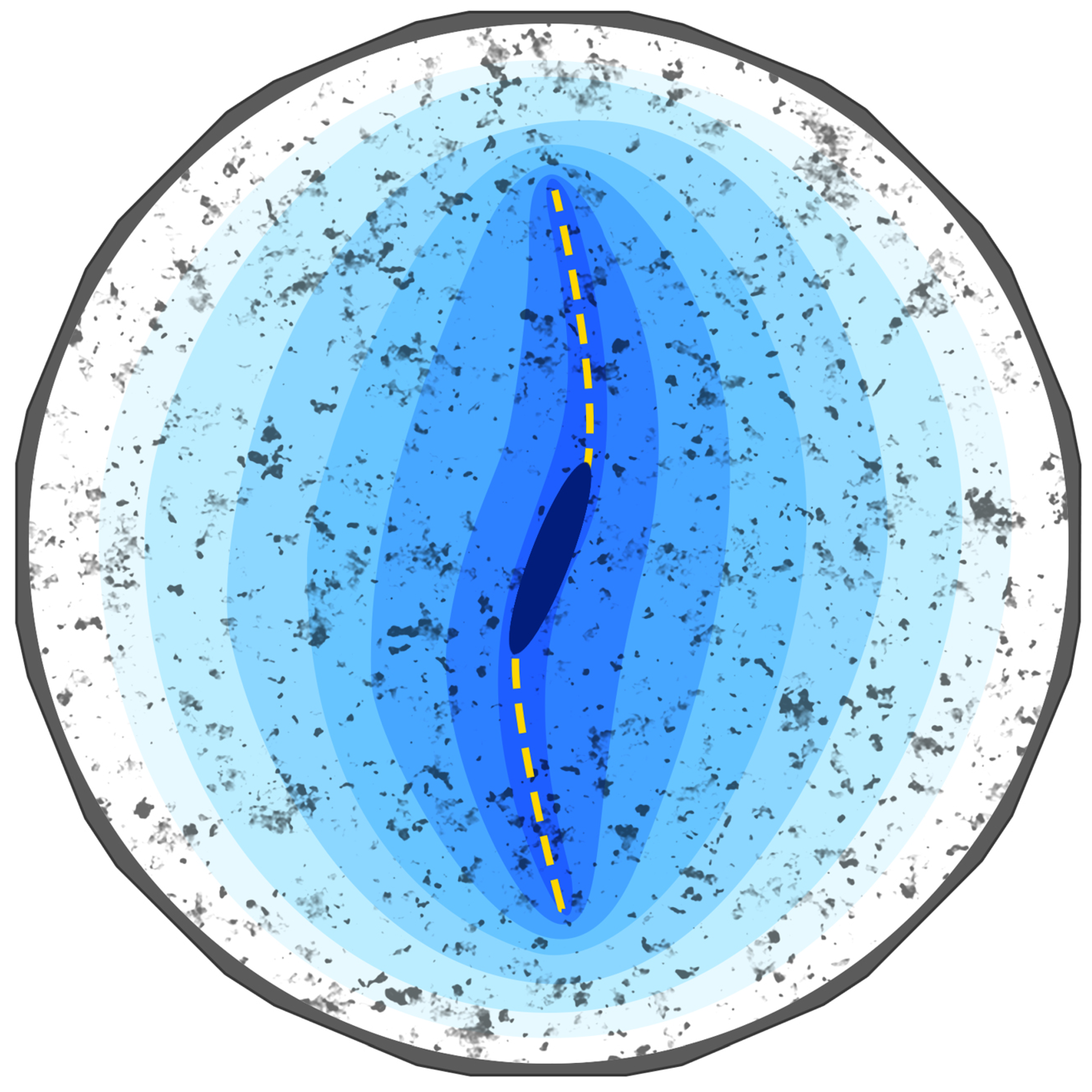
Figure 15 presents the phase field and pressure profiles under different loading conditions for the Greywacke sample at s after the start of injection. The results demonstrate the influence of poly-axial loading on the direction of fracture propagation. In all cases, it is evident that the direction of hydraulic fracturing tends to align parallel to the maximum stress at the boundaries.
In Scenario Load A, where the minimum principal stress is applied in the y-direction, the fracture primarily propagates perpendicular to this direction (Figure 15a). However, a slight counterclockwise deviation from the horizontal direction observed due to the effects of poly-axial loading. Although the maximum principal stress acts horizontally, the overall stress distribution (see Figure 4a) influences the fracture path, causing it to deviate slightly from a purely horizontal trajectory. In Scenario Load B, where the minimum principal stress is aligned with the fracture plane, the fracture deviates into direction of maximum principal stress (Figure 15b). In Scenario Load C, with the minimum principal stress applied in the x-direction, the hydraulic fracture predominantly propagates vertically (Figure 15c). Therefore, the computational results align well with expected hydraulic fracture propagation mechanisms, demonstrating that the numerical model effectively captures key processes governing hydraulic fracture evolution under different boundary conditions.
3.4.2. Hydraulic fracturing (borehole)–
In the final benchmark, a benchmark set is introduced where fractures nucleate from a borehole under various poly-axial conditions. The injection rate is set to m2/s at the borehole, where m. The material and fluid properties used in the simulations are detailed in Table 1 and Table 2. Note that no notch is considered in this case, and injection occurs directly inside the borehole.
Figure 16 displays the phase field and pressure profiles for the Greywacke sample under different loading conditions at s after injection began. The fracture nucleation and propagation tend to align parallel to the maximum overall stress at the boundaries.
4. Discussion
The VPF-FEM and LIE-FEM approaches are two different numerical methods of dealing with fracture problems. VPF-FEM is a smeared method; it represents fractures using a diffuse model represented by a phase-field variable. It is powerful because VPF-FEM can capture crack propagation without re-meshing, can handle crack branching and arbitrary crack paths, and is therefore suitable for modeling both fracture nucleation and propagation. However, to accurately capture the smeared fracture zone, a fine mesh resolution near the fracture is required. In contrast, the pre-existing fracture in LIE-FEM is explicitly embedded in the mesh and is therefore more discrete.
The primary distinction between these two approaches lies in their treatment of fracture mechanics. VPF-FEM does not explicitly define a fracture stiffness parameter; instead, it represents fractures using a degraded continuum approach, where stiffness gradually decreases based on a diffuse phase (damage) field. In contrast, LIE-FEM explicitly models fractures by incorporating stiffness parameters (), which dictate mechanical behavior under normal and shear loads. Regarding fracture propagation, both methods integrate fracture toughness but in different ways. In VPF-FEM, crack evolution is described through a phase-field variable, which captures the gradual transition from an intact material state to full fracture. This evolution is governed by an energy functional that incorporates fracture toughness, ensuring that crack propagation adheres to an energy-minimization principle, whereas LIE-FEM can employs cohesive zone models, where fracture toughness controls discrete fracture growth (though this aspect is not considered in this study). A notable advantage of VPF-FEM is its ability to model fracture nucleation, as demonstrated in benchmark , which examines hydraulic fracture initiation from a borehole. For shear behavior, VPF-FEM manages shear stiffness through energy decomposition, limiting independent control over shear strength. LIE-FEM, on the other hand, explicitly defines shear stiffness via , enabling independent control over shear resistance, even in closed fractures.
4.1. , – Intact rock samples
In the benchmark cases without fractures, and , the results obtained with VPF-FEM and LIE-FEM are identical. This consistency is attributed to the identical application of rotating boundary conditions in both methods and equivalence of their underlying poro-elastic model formulations.
Effect of initial conditions on hydro-mechanical model behavior
Accurate hydro-mechanical simulations require careful attention to sequential boundary conditions, especially in coupled fluid flow modeling for fractured media. In this study, a two-step approach is used to ensure numerical stability and physical accuracy. The first step includes a 3000 s steady-state phase under mechanical loading to allow the system to reach equilibrium (Figure 17b). This phase minimizes unrealistic pore pressure variations (e.g. Figure 17a) and establishes stable initial conditions for subsequent simulations. In the second step, a 500 s fluid injection phase is performed to model the flow dynamics. This sequential approach ensures that the effects of mechanical deformation are fully accounted for before fluid flow is introduced, a consideration that is especially critical in low-permeability media where strong coupling between fluid flow and deformation can lead to numerical instabilities. For VPF-FEM models, careful initialization is critical to achieving realistic fracture nucleation. Without proper initialization, artificial fracture nucleation can occur during the steady-state phase, leading to nonphysical results.
4.2. , – Fracture mechanics
In this set of benchmarks, the influence of an existing fracture on mechanical deformation is evaluated. For smaller fractures (), the volumetric strain measured along the probe circle shows strong agreement between VPF-FEM and LIE-FEM methods. However, for larger fractures (), where the fracture intersects the probe circle, both methods exhibit jumps in volumetric strain. While their results remain consistent at locations further from the fracture. To address this, three studies are conducted: the effect of mesh size in VPF-FEM, strain energy decomposition in VPF-FEM, and the impact of fracture stiffness in LIE-FEM.
Effect of mesh size in VPF-FEM
A mesh refinement analysis is performed for VPF-FEM to evaluate its behavior relative to LIE-FEM in modeling both volumetric strain and stress. Here, the Volumetric-Deviatoric strain energy decomposition is used in VPF-FEM. Figure 18a shows the volumetric strain at the probe circle for different mesh sizes, compared to LIE-FEM results. Figure 18b and Figure 18c illustrate the von Mises stress and strain along a vertical line perpendicular to the fracture at , highlighting the role of shear stress and strain in shaping these results. The findings reveal that mesh size does not significantly affect the magnitude of the volumetric strain jump. However, it can influence the maximum von Mises strain within the fracture (). These differences arise from fundamental variations in how each method models fractures. LIE-FEM explicitly represents fractures, whereas VPF-FEM uses a smeared phase-field approach, leading to smoother transitions. The LIE-FEM results are particularly sensitive to the fracture stiffness parameters ( for normal deformation and for shear deformation). In contrast, VPF-FEM results are strongly influenced by the strain energy decomposition choice.
Effect of strain energy decomposition approaches in VPF-FEM
To analyze the effect of strain energy decomposition on fracture behavior, the benchmark is repeated using four strain energy decomposition approaches for VPF-FEM (see Appendix H). Figure 19a presents the volumetric strain results, showing that the Isotropic and Volumetric-Deviatoric models exhibit volumetric strain jumps, similar with the LIE-FEM method, due to their ability to redistribute strain. In contrast, the Spectral and No-tension models display minimal volumetric strain jumps, as they confine fracture (propagation) strictly to tensile regions, preventing volumetric expansion near the crack zone. Figure 19b further illustrates the Von Mises stress distribution along the perpendicular line at (0,0) in the y-direction. It highlights that both Isotropic and Volumetric-Deviatoric approaches lead to nearly zero Von Mises stress and high Von Mises strain inside the fracture at .
Effect of fracture stiffness in LIE-FEM
is evaluated using the LIE-FEM method across different fracture stiffness values. The Figure 21 illustrates that as fracture stiffness increases, the magnitude of jumps in volumetric straining within the LIE-FEM method decreases.
In LIE-FEM, all fractures incorporate a tension cut-off mechanism, ensuring that no traction is transferred across a fracture once the normal traction becomes non-negative. This enforces the condition .
While the previous discussion highlights the performance differences between VPF-FEM and LIE-FEM, it is important to address an issue observed in the LIE-FEM method when using a quadrilateral mesh (see Figure A24a). This configuration introduces volumetric locking, which affects the accuracy of the strain and stress results. To address this, the B-bar method introduced by Hughes (1980) [79] has been used. However, this problem is not observed in the VPF-FEM method due to its formulation. More details on the B-bar method can be found in the Appendix G.
4.3. , – Effective permeability evolution under different poly-axial loading
This set of benchmarks evaluates the evolution of effective permeability under poly-axial loading, taking into account hydro-mechanical responses in the presence of fractures. Benchmarks and represent the most comprehensive scenarios, capturing the interactions between strain, fracture mechanics, and fluid flow. The volumetric strain plots for these cases indicate that both VPF-FEM and LIE-FEM can reproduce the hydro mechanical behavior of samples under different loading conditions.
The key concept explored here is the evolution of effective permeability under varying poly-axial loading conditions. In this setup, the fracture is oriented perpendicular to the main experimental element (PEE 5/5a, Figure 3b). As the angle between the second principal stress MPa and the PEE 5/5a plane increases, the normal stress acting on the fracture plane decreases monotonically. The normal stress for each load case is determined as follows:
where , , and takes values of (Figure 3b). Effective permeability at the fracture center is calculated for each loading condition (Table 3) using the cubic law for ideal parallel plate fractures [80], , where b represents the effective hydraulic aperture.
The results shown in Figure 22 illustrate the evolution of permeability for Graywacke and Gneiss samples under full and half wing fractures ( and ). As expected, fracture permeability decreases with increasing normal stress in the fracture plane, in agreement with theoretical predictions. In , the VPF-FEM method predicts larger permeabilities than the LIE-FEM method. However, in , the LIE-FEM method predicts higher permeabilities. Despite these differences, both methods show good agreement—not only are they of the same order, but the differences remain small. This slight variation is attributed to the nature of width calculation in each method.
4.4. , – Hydraulic Fracturing
This section focuses exclusively on hydraulic fracturing results obtained with the VPF-FEM method, as fracture propagation is not modeled with the LIE-FEM method. Two benchmarks are considered in this context: , which examines fracture propagation from a pre-existing fracture, and , which simulates fracture nucleation from a central borehole (Figure 3a). The breakdown (peak or failure) pressure, which marks the onset of fracture propagation, is analyzed for Gneiss and Graywacke samples under different loading conditions (Load A, B, C, Figure 4). The results for these scenarios are presented in Figure 23a and Figure 23b. In the absence of pre-existing fractures, as in , the breakdown pressure reflects a more realistic scenario where it is primarily determined by the material properties of the specimens rather than the poly-axial loading conditions. Conversely, in the presence of pre-existing fractures (, Figure 23a), the breakdown pressure varies slightly depending on the orientation of the applied load relative to pre-existing fracture. Specifically, when the maximum applied stress aligns with the fracture plane, the breakdown pressure is lower (Load A in Figure 23a) due to reduced resistance to propagation. In contrast, when the loading direction is nearly perpendicular to the fractures, the breakdown pressure increases because the stress concentration at the fracture tips is lower, making fracture initiation more difficult and delaying propagation.
5. Conclusions
Based on the GREAT cell experiments [24,25,26,81], a systematic collection of benchmarks has been developed to test various aspects of fracture mechanics for crystalline rocks (Gneiss and Graywacke). The special feature of the GREAT cell compared to conventional triaxial tests is that polyaxial stress ratios (rotating stress conditions) can be applied to the specimens, so that in particular fracture properties can be investigated under variable stress conditions as they may occur in geotechnical applications such as deep geothermal energy, energy storage, and disposal.
The benchmark types include intact rocks (, ) as well as symmetrically (, ) and asymmetrically fractured samples (, ). The benchmark types were simulated using two different fracture mechanics approaches, the variational phase field (VPF) and the lower interface element (LIE) methods, both implemented in the finite element method (FEM). The differences between diffuse and explicit representations of fracture in the context of mechanical and hydro-mechanical processes have been worked out (see below). In addition, fracture propagation processes have been analyzed using VPF-FEM method (, ).
Key findings from the comprehensive benchmark study include
- For the mechanical benchmarks and , sinusoidal strain patterns are successfully reproduced by both models. Gneiss exhibits smaller strain amplitudes due to its higher stiffness, while Graywacke exhibits larger total compressive strains.
- In static fracture modeling (, ), stress singularities are captured by both methods, showing good agreement far from the fracture. However, the magnitude of volumetric strain jumps, when the probe circle passes through the fracture, is affected by the choice of fracture stiffness in LIE-FEM and strain energy decomposition in VPF-FEM. Consistent global deformation responses are produced by both approaches.
- For the hydro-mechanical cases and , stress redistribution is affected by permeability variations, with normal stress at the fracture plane decreasing as the principal stress angle increases.
- For propagating fractures (and ), the direction of fracture propagation is accurately predicted by VPF-FEM, and the breakdown pressure is consistent with fracture mechanics expectations.
While LIE-FEM provides a more explicit representation of discontinuities, VPF-FEM excels in modeling fracture evolution. However, LIE-FEM is more computationally efficient because it increases the degrees of freedom only in the fracture regions, whereas VPF-FEM requires an additional phase field variable per node. In addition, LIE-FEM explicitly incorporates fracture stiffness, unlike VPF-FEM, which affects stress calculations at discontinuities. Despite previous analytical verification (see [22,30,43,65,68]), real-world inconsistencies persist due to differences in fracture width representation and fracture stiffness modeling, highlighting the need for further investigation.
This collection of benchmarks serves two purposes. First, it is a reference for model comparison with other fracture mechanics methods, such as discrete element methods, cellular automata, or, in the future, machine learning. On the other hand, it serves as a starting point for the evaluation of more complex GREAT cell experiments, e.g. considering 3D effects, fracture networks and anisotropic material behavior. The current benchmark collection initially covers mechanical and hydro-mechanical processes and will be extended to thermal processes in the next version as part of the DECOVALEX 2027 task SAFENET-2. This will allow to cover the whole range of thermo-hydro-mechanical (THM) fracture mechanics. The benchmark collection will also be successively published as a collection of Jupyter notebooks, thus facilitating the integration of further numerical methods and codes and contributing to open science.
Acknowledgments
DECOVALEX (https://decovalex.org) is an international research collaboration that unites industry, government, and academia to enhance the understanding and modeling of complex subsurface geological and engineering processes. The initiative is currently progressing through its DECOVALEX-2027 phase. The authors also wish to extend their gratitude to the core development team of OpenGeoSys software for their invaluable contributions to the implementation process. The first author (MM) would like to express his deepest gratitude to Dr. Keita Yoshioka for his careful review of the manuscript and invaluable feedback. Provision of experimental data from the GREAT cell partially supported through the UK Engineering and Physical Sciences Research Council (EPSRC) for the project “Smart Pumping for Subsurface Engineering” grant number (EP/S005560/1) is gratefully acknowledged. This work has been co-financed within the framework of the Federal Ministry of Education and Research (BMBF) project “Digitisation and automation of benchmarking workflows for geoscientific process simulations – DigBen” (Grant No 03G0927A), this support is gratefully acknowledged. This work is also contributing to the European Joint Programme on Radioactive Waste Management EURAD “European Partnership on Radioactive Waste Management” (Grant Agreement No 101166718).
Appendix F Jupyter notebooks
The ongoing SAFENET Task within DECOVALEX 2027 will also develop new approaches to benchmarking by following the FAIR principles, i.e. that future benchmarks will be Findable, Accessible, Interoperable and Reproducible. Status quo is that benchmarks are described in publications but only a few are available online as provided by the OpenGeoSys benchmarking gallery1, e.g. for static fracture opening under a constant pressure by Sneddon solution2 [82].
The current test case from this paper are available as executeable Jupyter notebooks, https://github.com/wenqing/GreatCell-benchmarks-2024.
Appendix G Numerical benchmarks considerations
This section highlights numerical strategies for replicating the responses of intact and fractured samples, ensuring accurate behavior modeling with computational efficiency.
- VPF-FEM
-
Fracture states
- –
- Intact matrix: The phase field is uniformly set to 1, effectively suppressing fracture initiation. High fracture toughness is applied to ensure that no fracture propagation occurs.
- –
- Static pre-existing fracture: The phase field is set to 0 in the fracture region and 1 elsewhere, representing a static, non-propagating fracture. The fracture length scale is defined as , where corresponds to the smallest mesh element size.
- –
- Propagating fracture: The material is assigned its nominal fracture toughness, enabling the fracture to propagate under appropriate stress and fluid pressure conditions.
-
Fluid dynamics and matrix interaction
- –
-
No fluid flow (mechanical):
- *
- Fluid injection and pressure boundary conditions are absent, effectively isolating the influence of fluid dynamics.
- *
- The matrix is assumed to be rigid (), resulting in the decoupling of pore pressure from mechanical deformation.
- *
- A high permeability () is prescribed to negate the effects of fluid flow.
- –
-
Fluid flow (hydro-mechanical):
- –
- Fluid is introduced along a line source (in fracture) at a rate of , corresponding to a total injection rate of . In intact samples, since there are no fractures, the fluid is simply injected at a source point.
- –
- A constant pressure boundary condition is imposed along an outlet with a length of h.
- –
- Fluid pressure evolution and its interaction with mechanical deformation are governed by matrix permeability and poro-elastic coupling, characterized by the Biot coefficient.
- LIE–FEM
The numerical accuracy of the LIE method has been improved by the B-bar method [79]. Figure A24 compares the stress magnitude obtained using the LIE-FEM method with and without the B-bar method. It can be seen from Figure A24 that the stress pattern obtained without the B-bar shows significant numerical artifacts, whereas the one obtained with the B-bar shows no numerical artifacts.
Figure A24.
: Comparison of stress and strain traces results obtained with and without the B-bar method under Load F (LIE-FEM).
Figure A24.
: Comparison of stress and strain traces results obtained with and without the B-bar method under Load F (LIE-FEM).
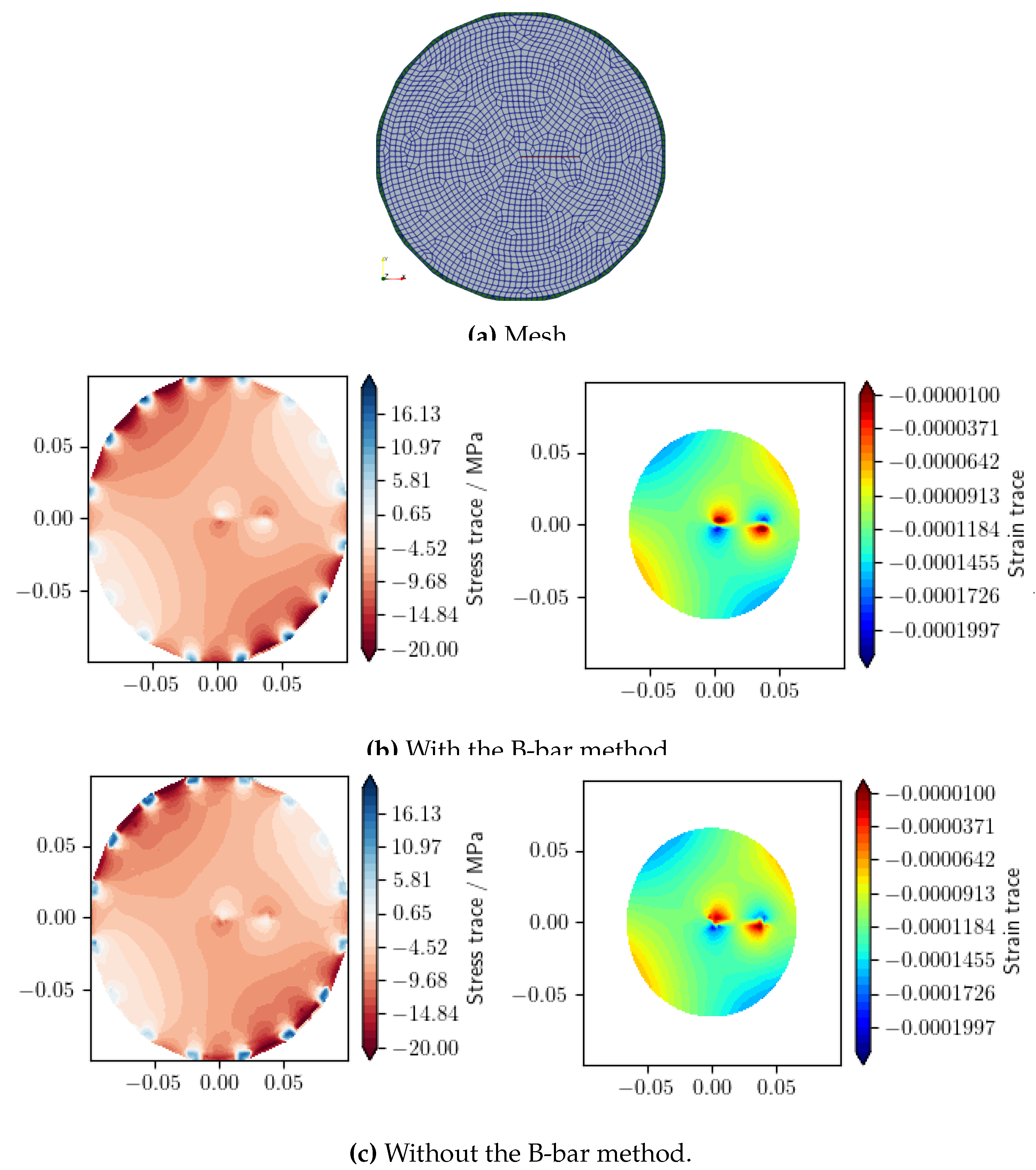
Figure A25 compares the obtained strain profiles obtained with and without the B-bar method, which shows that the B-bar method eliminates the oscillation in the profile curve for the simulation without the B-bar method.
Figure A25.
: Strain profiles obtained using the LIE method with and without the B-bar method under Load F (LIE-FEM).
Figure A25.
: Strain profiles obtained using the LIE method with and without the B-bar method under Load F (LIE-FEM).
Appendix H Strain energy decompositions approaches in VPF-FEM
The strain energy decomposition in the variational phase-field framework is given by:
where is the degradation function, and the strain energy is divided into positive (tensile) and negative (compressive) components. For a more detailed discussion on the implementation of strain energy decomposition in the variational phase-field method, see [83,84]. Below, we outline four representative strain energy decomposition models used in VPF-FEM.
- Isotropic model [49]: This model applies uniform degradation to the total strain energy. It does not distinguish between tensile and compressive contributions, leading to uniform degradation across shear, tensile, and compressive stiffness. Consequently, shear strength cannot be independently controlled.
-
Volumetric-Deviatoric decomposition approach [85]: This model introduces a decomposition into volumetric and deviatoric components. While degradation primarily affects the deviatoric strain energy, positive volumetric strain energy is also subjected to degradation, whereas negative volumetric strain energy remains unaffected. However, shear strength remains intrinsically linked to tensile strength, preventing independent control.Here, represents the deviatoric part of the strain tensor and the symbols and represent the positive and negative parts, respectively, of the trace of the strain tensor, defined as .
- Spectral decomposition approach [86]: This model refines this separation by decomposing the strain tensor into tensile () and compressive () contributions using eigenvalue analysis. The strain tensor is diagonalized in its principal basis as , where are the principal strains (eigenvalues of ), and are the projection tensors, aligned with the eigenvectors . The strain energy decomposition defines aswhich ensures that fracture propagation is driven exclusively by tensile stress while preserving compressive energy. Although this method offers more flexibility in shear strength control, it does not achieve complete decoupling from tensile strength [84].
-
No-Tension decomposition approach [87]: This approach enforces a strict no-tension condition by decomposing the strain tensor into tensile and compressive parts while ensuring that the tensile strain remains a positive semi-definite tensor. The strain is decomposed as where . Therefore, the strain energy decomposition defines asThis model suppresses crack evolution under compressive loads. However, residual stresses introduce the same coupling issues as in the Spectral split, and shear strength remains dependent on tensile behavior [84].
| 1 | |
| 2 |
References
- Birkholzer, J.T.; Bond, A.E.; Hudson, J.A.; Jing, L.; Tsang, C.F.; Shao, H.; Kolditz, O. DECOVALEX-2015: an international collaboration for advancing the understanding and modeling of coupled thermo-hydro-mechanical-chemical (THMC) processes in geological systems. Environmental Earth Sciences 2018, 77. [Google Scholar] [CrossRef]
- Birkholzer, J.T.; Tsang, C.F.; Bond, A.E.; Hudson, J.A.; Jing, L.; Stephansson, O. 25 years of DECOVALEX - Scientific advances and lessons learned from an international research collaboration in coupled subsurface processes. International Journal of Rock Mechanics and Mining Sciences 2019, 122. [Google Scholar] [CrossRef]
- Kolditz, O.; Fischer, T.; Frühwirt, T.; Görke, U.J.; Helbig, C.; Konietzky, H.; Maßmann, J.; Nest, M.; Pötschke, D.; Rink, K.; et al. GeomInt: geomechanical integrity of host and barrier rocks–experiments, models and analysis of discontinuities. Environmental Earth Sciences 2021, 80. [Google Scholar] [CrossRef]
- Birkholzer, J.T.; Bond, A.E. DECOVALEX-2019: An international collaboration for advancing the understanding and modeling of coupled thermo-hydro-mechanical-chemical (THMC) processes in geological systems. International Journal of Rock Mechanics and Mining Sciences 2022, 154. [Google Scholar] [CrossRef]
- Birkholzer, J.T.; Bond, A.E.; Tsang, C.F. The DECOVALEX international collaboration on modeling of coupled subsurface processes and its contribution to confidence building in radioactive waste disposal. Hydrogeology Journal 2024. [Google Scholar] [CrossRef]
- Nguyen, T.S.; Kolditz, O.; Yoon, J.S.; Zhuang, L. Modelling the thermo-mechanical behaviour of a rock joint. Geomechanics for Energy and the Environment 2024, 37, 100520. [Google Scholar] [CrossRef]
- Park, J.W.; Park, C.H.; Zhuang, L.; Yoon, J.S.; Kolditz, O.; McDermott, C.I.; Park, E.S.; Lee, C. Grain-based distinct element modeling of thermally induced slip of critically stressed rock fracture. Geomechanics for Energy and the Environment 2024, 39, 100580. [Google Scholar] [CrossRef]
- Chang, C.C.; Chiou, Y.F.; Shen, Y.H.; Yu, Y.C. Modelling of mass transport in fractured crystalline rock using velocity interpolation and cell-jump particle tracking methods. Geomechanics for Energy and the Environment 2024, 40, 100615. [Google Scholar] [CrossRef]
- Pitz, M.; Grunwald, N.; Graupner, B.; Kurgyis, K.; Radeisen, E.; Maßmann, J.; Ziefle, G.; Thiedau, J.; Nagel, T. Benchmarking a new TH2M implementation in OGS-6 with regard to processes relevant for nuclear waste disposal. Environmental Earth Sciences 2023, 82. [Google Scholar] [CrossRef]
- Sasaki, T.; Yoon, S.; Rutqvist, J. Modelling of failure and fracture development of the Callovo-Oxfordian claystone during an in-situ heating experiment associated with geological disposal of high-level radioactive waste. Geomechanics for Energy and the Environment 2024, 38, 100546. [Google Scholar] [CrossRef]
- Rodriguez-Dono, A.; Zhou, Y.; Olivella, S.; Gens, A. Modelling a gas injection experiment incorporating embedded fractures and heterogeneous material properties. Geomechanics for Energy and the Environment 2024, 38, 100552. [Google Scholar] [CrossRef]
- Song, F.; Gens, A.; Collico, S.; Plúa, C.; Armand, G.; Wang, H. Analysis of thermally-induced fracture of Callovo-Oxfordian claystone: From lab tests to field scale. Geomechanics for Energy and the Environment 2024, 39, 100579. [Google Scholar] [CrossRef]
- Kuhlman, K.L.; Bartol, J.; Benbow, S.J.; Bourret, M.; Czaikowski, O.; Guiltinan, E.; Jantschik, K.; Jayne, R.; Norris, S.; Rutqvist, J.; et al. Synthesis of results for Brine Availability Test in Salt (BATS) DECOVALEX-2023 Task E. Geomechanics for Energy and the Environment 2024, 39, 100581. [Google Scholar] [CrossRef]
- Noghretab, B.; Damians, I.; Olivella, S.; Gens, A. Coupled Hydro-Gas-Mechanical 3D Modeling of LASGIT Experiment. Geomechanics for Energy and the Environment 2024, 100623. [Google Scholar] [CrossRef]
- Wang, J.; Chen, L.; Su, R.; Zhao, X. The Beishan underground research laboratory for geological disposal of high-level radioactive waste in China: planning, site selection, site characterization and in situ tests. Journal of Rock Mechanics and Geotechnical Engineering 2018, 10, 411–435. [Google Scholar] [CrossRef]
- Frank, T.; Becker, D.A.; Benbow, S.; Bond, A.; Jayne, R.; LaForce, T.; Wolf, J. Value of abstraction in performance assessment – When is a higher level of detail necessary? Geomechanics for Energy and the Environment 2024, 39, 100577. [Google Scholar] [CrossRef]
- Hu, G.; Schoenball, M.; Pfingsten, W. Machine learning-assisted heat transport modelling for full-scale emplacement experiment at Mont Terri underground laboratory. International Journal of Heat and Mass Transfer 2023, 213. [Google Scholar] [CrossRef]
- Hu, G.; Pfingsten, W. Data-driven machine learning for disposal of high-level nuclear waste: A review. Annals of Nuclear Energy 2023, 180. [Google Scholar] [CrossRef]
- Li, M.; Wu, Z.; Weng, L.; Zhang, F.; Zhou, Y.; Wu, Y. Cross-scale analysis for the thermo-hydro-mechanical (THM) effects on the mechanical behaviors of fractured rock: Integrating mesostructure-based DEM modeling and machine learning. Engineering Fracture Mechanics 2024, 306. [Google Scholar] [CrossRef]
- Hu, G.; Prasianakis, N.; Churakov, S.V.; Pfingsten, W. Performance analysis of data-driven and physics-informed machine learning methods for thermal-hydraulic processes in Full-scale Emplacement experiment. Applied Thermal Engineering 2024, 245. [Google Scholar] [CrossRef]
- Kolditz, O.; McDermott, C.; Yoon, J.S.; Mollaali, M.; Wang, W.; Hu, M.; Sasaki, T.; Rutqvist, J.; Birkholzer, J.; Park, J.W.; et al. A systematic model and experimental approach to hydro-mechanical and thermo-mechanical fracture processes in crystalline rocks. Geomechanics for Energy and the Environment 2024, 100616. [Google Scholar] [CrossRef]
- Mollaali, M.; Kolditz, O.; Hu, M.; Park, C.H.; Park, J.W.; McDermott, C.I.; Chittenden, N.; Bond, A.; Yoon, J.S.; Zhou, J.; et al. Comparative verification of hydro-mechanical fracture behavior: Task G of international research project DECOVALEX–2023. International Journal of Rock Mechanics and Mining Sciences 2023, 170. [Google Scholar] [CrossRef]
- Frühwirt, T.; Pötschke, D.; Konietzky, H. Simulation of direct shear tests using a forces on fracture surfaces (FFS) approach. Environmental Earth Sciences 2021, 80. [Google Scholar] [CrossRef]
- McDermott, C.; Fraser-Harris, A.; Sauter, M.; Couples, G.; Edlmann, K.; Kolditz, O.; Lightbody, A.; Somerville, J.; Wang, W. New Experimental Equipment Recreating Geo-Reservoir Conditions in Large, Fractured, Porous Samples to Investigate Coupled Thermal, Hydraulic and Polyaxial Stress Processes. Scientific Reports 2018, 8. [Google Scholar] [CrossRef] [PubMed]
- Fraser-Harris, A.; Lightbody, A.; Edlmann, K.; Elphick, S.; Couples, G.; Sauter, M.; McDermott, C. Sampling and preparation of c.200 mm diameter cylindrical rock samples for geomechanical experiments. International Journal of Rock Mechanics and Mining Sciences 2020, 128. [Google Scholar] [CrossRef]
- Fraser-Harris, A.; McDermott, C.; Couples, G.; Edlmann, K.; Lightbody, A.; Cartwright-Taylor, A.; Kendrick, J.; Brondolo, F.; Fazio, M.; Sauter, M. Experimental Investigation of Hydraulic Fracturing and Stress Sensitivity of Fracture Permeability Under Changing Polyaxial Stress Conditions. Journal of Geophysical Research: Solid Earth 2020, 125. [Google Scholar] [CrossRef]
- Sun, C.; Zhuang, L.; Jung, S.; Lee, J.; Yoon, J.S. Thermally induced slip of a single sawcut granite fracture under biaxial loading. Geomechanics and Geophysics for Geo-Energy and Geo-Resources 2021, 7. [Google Scholar] [CrossRef]
- Sun, C.; Zhuang, L.; Yoon, J.S.; Min, K.B. Thermally induced shear reactivation of critically-stressed smooth and rough granite fractures. IOP Conference Series: Earth and Environmental Science 2023, 1124. [Google Scholar] [CrossRef]
- Sun, C.; Zhuang, L.; Youn, D.J.; Yoon, J.S.; Min, K.B. Laboratory investigation of thermal stresses in fractured granite: Effects of fracture surface roughness and initial stress. TUNNELLING AND UNDERGROUND SPACE TECHNOLOGY 2024, 145. [Google Scholar] [CrossRef]
- Yoshioka, K.; Parisio, F.; Naumov, D.; Lu, R.; Kolditz, O.; Nagel, T. Comparative verification of discrete and smeared numerical approaches for the simulation of hydraulic fracturing. GEM - International Journal on Geomathematics 2019, 10. [Google Scholar] [CrossRef]
- Belytschko, T.; Black, T. Elastic crack growth in finite elements with minimal remeshing. International journal for numerical methods in engineering 1999, 45, 601–620. [Google Scholar] [CrossRef]
- Linder, C.; Armero, F. Finite elements with embedded strong discontinuities for the modeling of failure in solids. International Journal for Numerical Methods in Engineering 2007, 72, 1391–1433. [Google Scholar] [CrossRef]
- Feist, C.; Hofstetter, G. An embedded strong discontinuity model for cracking of plain concrete. Computer Methods in Applied Mechanics and Engineering 2006, 195, 7115–7138. [Google Scholar] [CrossRef]
- Ibrahimbegovic, A.; Melnyk, S. Embedded discontinuity finite element method for modeling of localized failure in heterogeneous materials with structured mesh: an alternative to extended finite element method. Computational Mechanics 2007, 40, 149–155. [Google Scholar] [CrossRef]
- Rangarajan, R. Universal Meshes, a New Paradigm for Computing with Nonconforming Triangulations; Stanford University, 2012.
- Hunsweck, M.J.; Shen, Y.; Lew, A.J. A finite element approach to the simulation of hydraulic fractures with lag. International Journal for Numerical and Analytical Methods in Geomechanics 2013, 37, 993–1015. [Google Scholar] [CrossRef]
- Mollaali, M.; Ziaei-Rad, V.; Shen, Y. Numerical modeling of CO_2 fracturing by the phase field approach. Journal of Natural Gas Science and Engineering 2019, 70, 102905. [Google Scholar] [CrossRef]
- Bažant, Z.P.; Oh, B.H. Crack band theory for fracture of concrete. Matériaux et construction 1983, 16, 155–177. [Google Scholar] [CrossRef]
- Peerlings, R.H.; Geers, M.G.; de Borst, R.; Brekelmans, W. A critical comparison of nonlocal and gradient-enhanced softening continua. International Journal of solids and Structures 2001, 38, 7723–7746. [Google Scholar] [CrossRef]
- Bourdin, B.; Francfort, G.; Marigo, J.J. Numerical experiments in revisited brittle fracture. Journal of the Mechanics and Physics of Solids 2000, 48, 797–826. [Google Scholar] [CrossRef]
- Nagel, T.; Gerasimov, T.; Remes, J.; Kern, D. Neighborhood Watch in Mechanics: Nonlocal Models and Convolution. SIAM Review 2025, 67, 176–193. [Google Scholar] [CrossRef]
- Francfort, G.A.; Marigo, J.J. Revisiting brittle fracture as an energy minimization problem. Journal of the Mechanics and Physics of Solids 1998, 46, 1319–1342. [Google Scholar] [CrossRef]
- Watanabe, N.; Wang, W.; Taron, J.; Görke, U.; Kolditz, O. Lower-dimensional interface elements with local enrichment: Application to coupled hydro-mechanical problems in discretely fractured porous media. International Journal for Numerical Methods in Engineering 2012, 90, 1010–1034. [Google Scholar] [CrossRef]
- Bilke, L.; Naumov, D.; Wang, W.; Fischer, T.; Lehmann, C.; Buchwald, J.; Shao, H.; Kiszkurno, F.K.; Chen, C.; Silbermann, C.; et al. OpenGeoSys. https://zenodo.org/records/10890088, 2024.
- Bilke, L.; Flemisch, B.; Kalbacher, T.; Kolditz, O.; Helmig, R.; Nagel, T. Development of Open-Source Porous Media Simulators: Principles and Experiences. Transport in Porous Media 2019, 130, 337–361. [Google Scholar] [CrossRef]
- Kolditz, O.; Jacques, D.; Claret, F.; Bertrand, J.; Churakov, S.V.; Debayle, C.; Diaconu, D.; Fuzik, K.; Garcia, D.; Graebling, N.; et al. Digitalisation for nuclear waste management: predisposal and disposal. Environmental Earth Sciences 2023, 82. [Google Scholar] [CrossRef]
- Biot, M.A. General theory of three-dimensional consolidation. Journal of Applied Physics 1941, 12, 155–164. [Google Scholar] [CrossRef]
- Ambati, M.; Gerasimov, T.; De Lorenzis, L. Phase-field modeling of ductile fracture. Computational Mechanics 2015, 55, 1017–1040. [Google Scholar] [CrossRef]
- Bourdin, B.; Francfort, G.; Marigo, J.J. The variational approach to fracture. Journal of Elasticity 2008, 91, 5–148. [Google Scholar] [CrossRef]
- Tanné, E.; Li, T.; Bourdin, B.; Marigo, J.J.; Maurini, C. Crack nucleation in variational phase-field models of brittle fracture. Journal of the Mechanics and Physics of Solids 2018, 110, 80–99. [Google Scholar] [CrossRef]
- Yoshioka, K.; Mollaali, M.; Kolditz, O. Variational phase-field fracture modeling with interfaces. Computer Methods in Applied Mechanics and Engineering 2021, 384, 113951. [Google Scholar] [CrossRef]
- Gerasimov, T.; De Lorenzis, L. On penalization in variational phase-field models of brittle fracture. Computer Methods in Applied Mechanics and Engineering 2019, 354, 990–1026. [Google Scholar] [CrossRef]
- Ziaei-Rad, V.; Mollaali, M.; Nagel, T.; Kolditz, O.; Yoshioka, K. Orthogonal decomposition of anisotropic constitutive models for the phase field approach to fracture. Journal of the Mechanics and Physics of Solids 2023, 171, 105143. [Google Scholar] [CrossRef]
- Dittmann, M.; Aldakheel, F.; Schulte, J.; Wriggers, P.; Hesch, C. Variational phase-field formulation of non-linear ductile fracture. Computer Methods in Applied Mechanics and Engineering 2018, 342, 71–94. [Google Scholar] [CrossRef]
- Ambati, M.; Gerasimov, T.; De Lorenzis, L. Phase-field modeling of ductile fracture. Computational Mechanics 2015, 55, 1017–1040. [Google Scholar] [CrossRef]
- Lo, Y.S.; Borden, M.J.; Ravi-Chandar, K.; Landis, C.M. A phase-field model for fatigue crack growth. Journal of the Mechanics and Physics of Solids 2019, 132, 103684. [Google Scholar] [CrossRef]
- Simoes, M.; Martinez-Paneda, E. Phase field modelling of fracture and fatigue in Shape Memory Alloys. Computer Methods in Applied Mechanics and Engineering 2021, 373, 113504. [Google Scholar] [CrossRef]
- Xie, Q.; Qi, H.; Li, S.; Yang, X.; Shi, D.; Li, F. Phase-field fracture modeling for creep crack. Theoretical and Applied Fracture Mechanics 2023, 124, 103798. [Google Scholar] [CrossRef]
- Borden, M.; Verhoosel, C.; Scott, M.; Hughes, T.; Landis, C. A phase-field description of dynamic brittle fracture. Computer Methods in Applied Mechanics and Engineering 2012, 217-220, 77–95. [Google Scholar] [CrossRef]
- Nguyen, V.P.; Wu, J.Y. Modeling dynamic fracture of solids with a phase-field regularized cohesive zone model. Computer Methods in Applied Mechanics and Engineering 2018, 340, 1000–1022. [Google Scholar] [CrossRef]
- Bourdin, B.; Larsen, C.J.; Richardson, C.L. A time-discrete model for dynamic fracture based on crack regularization. International Journal of Fracture 2011, 168, 133–143. [Google Scholar] [CrossRef]
- Cajuhi, T.; Ziefle, G.; Maßmann, J.; Nagel, T.; Yoshioka, K. Modeling desiccation cracks in Opalinus Clay at field scale with the phase-field approach. InterPore Journal 2024, 1, ipj260424–7. [Google Scholar] [CrossRef]
- Heider, Y.; Sun, W. A phase field framework for capillary-induced fracture in unsaturated porous media: Drying-induced vs. hydraulic cracking. Computer Methods in Applied Mechanics and Engineering 2020, 359, 112647. [Google Scholar] [CrossRef]
- Chukwudozie, C.; Bourdin, B.; Yoshioka, K. A variational phase-field model for hydraulic fracturing in porous media. Computer Methods in Applied Mechanics and Engineering 2019, 347, 957–982. [Google Scholar] [CrossRef]
- You, T.; Yoshioka, K. On poroelastic strain energy degradation in the variational phase-field models for hydraulic fracture. Computer Methods in Applied Mechanics and Engineering 2023, 416, 116305. [Google Scholar] [CrossRef]
- Mollaali, M.; Shen, Y. An Elrod–Adams-model-based method to account for the fluid lag in hydraulic fracturing in 2D and 3D. International Journal of Fracture 2018, 211, 183–202. [Google Scholar] [CrossRef]
- Clavijo, S.P.; Addassi, M.; Finkbeiner, T.; Hoteit, H. A coupled phase-field and reactive-transport framework for fracture propagation in poroelastic media. Scientific Reports 2022, 12, 17819. [Google Scholar] [CrossRef] [PubMed]
- Mollaali, M.; Yoshioka, K.; Lu, R.; Montoya, V.; Vilarrasa, V.; Kolditz, O. Variational Phase-Field Fracture Approach in Reactive Porous Media. International Journal for Numerical Methods in Engineering 2025, 126, e7621. [Google Scholar] [CrossRef]
- Yoshioka, K.; Mollaali, M.; Mishaan, G.; Makhnenko, R.; Parisio, F. Impact of grain and interface fracture surface energies on fracture propagation in granite. In Proceedings of the ARMA US Rock Mechanics/Geomechanics Symposium. ARMA, pp. ARMA–2021; 2021. [Google Scholar]
- Mollaali, M.; Buchwald, J.; Montoya, V.; Kolditz, O.; Yoshioka, K. Clay–rock fracturing risk assessment under high gas pressures in repository systems. IOP Conference Series: Earth and Environmental Science 2023, 1124, 012120. [Google Scholar] [CrossRef]
- Yu, Z.; Shao, J.F.; Duveau, G.; Wang, M.; Vu, M.N.; Plua, C. Numerical modeling of gas injection induced cracking with unsaturated hydromechanical process in the context of radioactive waste disposal. Tunnelling and Underground Space Technology 2024, 146, 105609. [Google Scholar] [CrossRef]
- Henry, H.; Adda-Bedia, M. Fractographic aspects of crack branching instability using a phase-field model. Physical Review E 2013, 88, 060401. [Google Scholar] [CrossRef]
- Ma, L.; Mollaali, M.; Dugnani, R. Phase-field simulation of fractographic features formation in soda–lime glass beams fractured in bending. Theoretical and Applied Fracture Mechanics 2023, 127, 103997. [Google Scholar] [CrossRef]
- Griffith, A. The phenomenom of rupture and flow in solids Philos. TransR Soc London Ser A 1920, 221, 168–98. [Google Scholar]
- Biot, M. General Theory of Three-Dimensional Consolidation. Journal of Applied Physics 1941, 12, 155–164. [Google Scholar] [CrossRef]
- Shao, J. Poroelastic behaviour of brittle rock materials with anisotropic damage. Mechanics of Materials 1998, 30, 41–53. [Google Scholar] [CrossRef]
- Cheng, A.D. Material coefficients of anisotropic poroelasticity. International Journal of Rock Mechanics and Mining Sciences 1997, 34, 199–205. [Google Scholar] [CrossRef]
- Yi, L.P.; Waisman, H.; Yang, Z.Z.; Li, X.G. A consistent phase field model for hydraulic fracture propagation in poroelastic media. Computer Methods in Applied Mechanics and Engineering 2020, 372, 113396. [Google Scholar] [CrossRef]
- Hughes, T.J. Generalization of selective integration procedures to anisotropic and nonlinear media. International Journal for Numerical Methods in Engineering 1980, 15, 1413–1418. [Google Scholar] [CrossRef]
- Witherspoon, P.; Wang, J.; Iwai, K.; Gale, J. Validity of Cubic Law for fluid flow in a deformable rock fracture. Water Resources Research 1980, 16, 1016–1024. [Google Scholar] [CrossRef]
- Fraser-Harris, A.; Graham, S.; McDermott, C.; Lightbody, A.; Sauter, M. The influence of intermediate principal stress magnitude and orientation on fracture fluid flow characteristics of a fractured crystalline rock. in preparation 2024. [Google Scholar]
- Sneddon, I.; Lowengrub, M. Crack problems in the classical theory of elasticity; The SIAM series in Applied Mathematics; John Wiley & Sons, 1969. [Google Scholar]
- Shen, Y.; Mollaali, M.; Li, Y.; Ma, W.; Jiang, J. Implementation details for the phase field approaches to fracture. Journal of Shanghai Jiaotong University (Science) 2018, 23, 166–174. [Google Scholar] [CrossRef]
- Vicentini, F.; Zolesi, C.; Carrara, P.; Maurini, C.; De Lorenzis, L. On the energy decomposition in variational phase-field models for brittle fracture under multi-axial stress states. International Journal of Fracture 2024, 1–27. [Google Scholar] [CrossRef]
- Amor, H.; Marigo, J.J.; Maurini, C. Regularized formulation of the variational brittle fracture with unilateral contact: Numerical experiments. Journal of the Mechanics and Physics of Solids 2009, 57, 1209–1229. [Google Scholar] [CrossRef]
- Miehe, C.; Hofacker, M.; Welschinger, F. A phase field model for rate-independent crack propagation: Robust algorithmic implementation based on operator splits. Computer Methods in Applied Mechanics and Engineering 2010, 199, 2765–2778. [Google Scholar] [CrossRef]
- Freddi, F.; Royer-Carfagni, G. Regularized variational theories of fracture: A unified approach. Journal of the Mechanics and Physics of Solids 2010, 58, 1154–1174. [Google Scholar] [CrossRef]
Figure 3.
GREAT cell benchmarking concept for 2D plane-strain conditions: Sample types and rotating boundary conditions
Figure 3.
GREAT cell benchmarking concept for 2D plane-strain conditions: Sample types and rotating boundary conditions
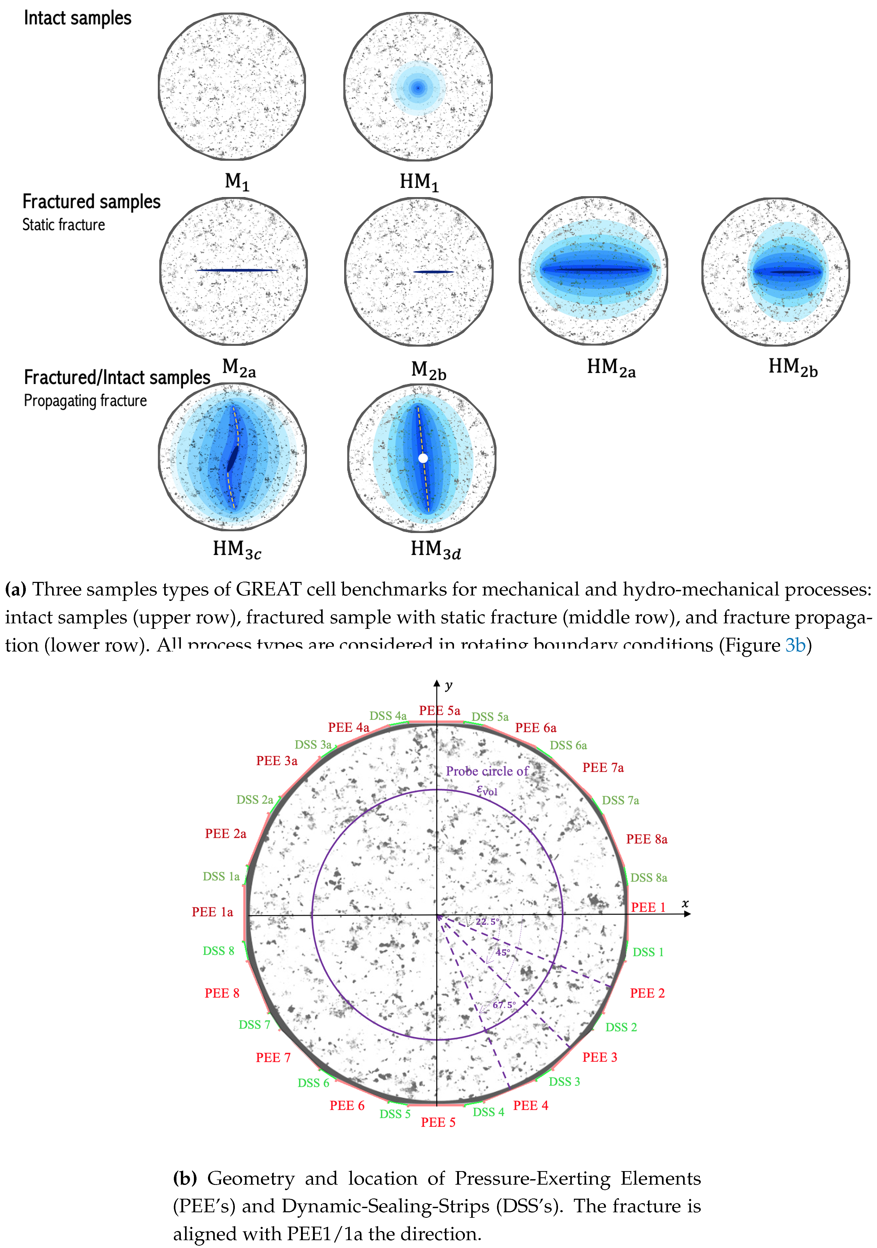
Figure 4.
Schematic of loading applied to the GREAT cell for loads A, B, and C (see Table 3). For simplicity in the figure, the DDS load is not included but can be approximated by the average of the stresses applied to the adjacent PEE’s. (Load unit: MPa).
Figure 4.
Schematic of loading applied to the GREAT cell for loads A, B, and C (see Table 3). For simplicity in the figure, the DDS load is not included but can be approximated by the average of the stresses applied to the adjacent PEE’s. (Load unit: MPa).
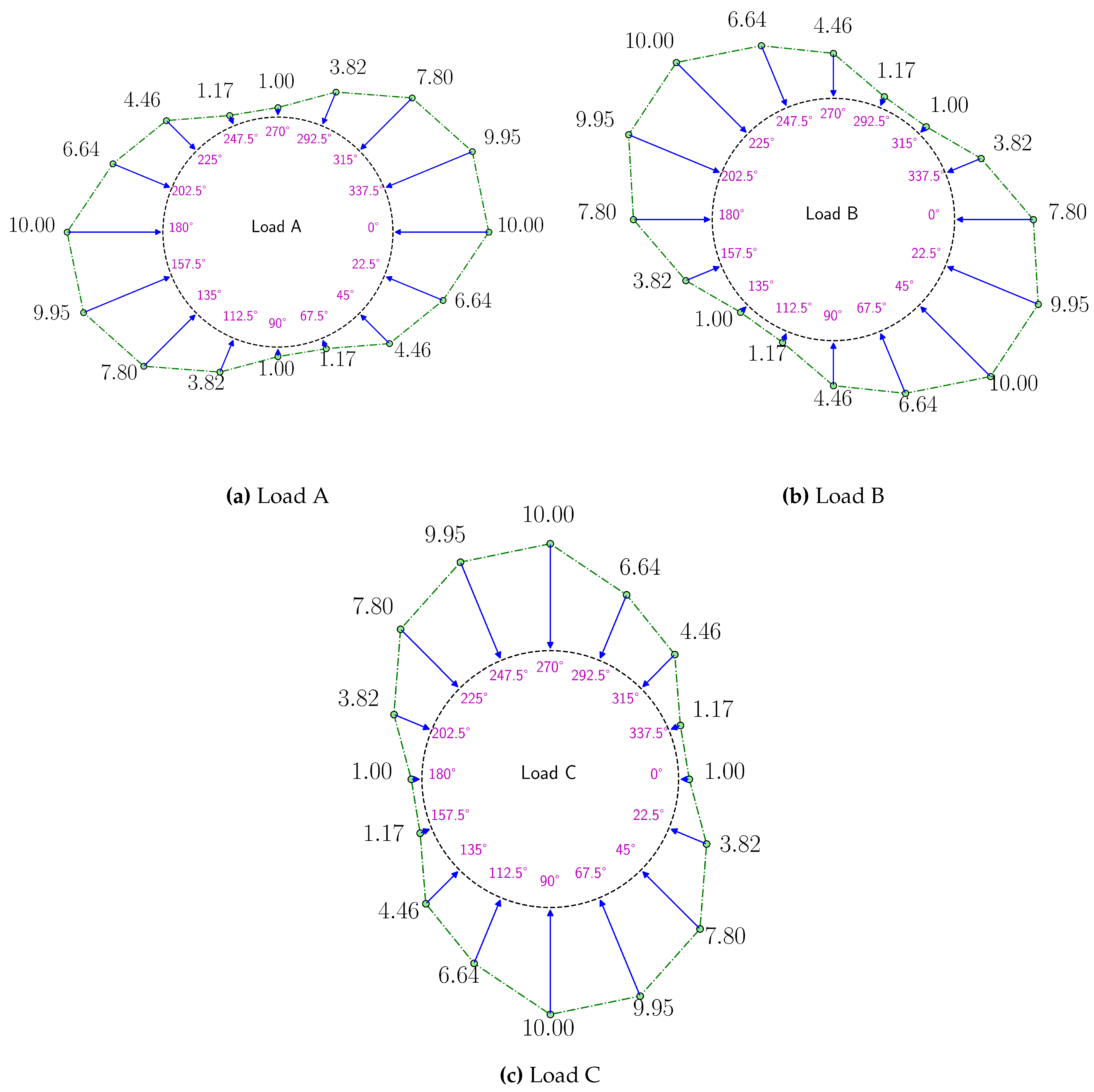
Figure 5.
: Trace of effective stress and volumetric strain versus angle for intact samples: (a) Greywacke and (b) Gneiss, under Load A (Table 1 ) at the final time (VPF-FEM). For the volumetric strain, the results for , where the strain is higher due to the softness of the PEE’s, are deactivated to focus on the region near the core of the sample.
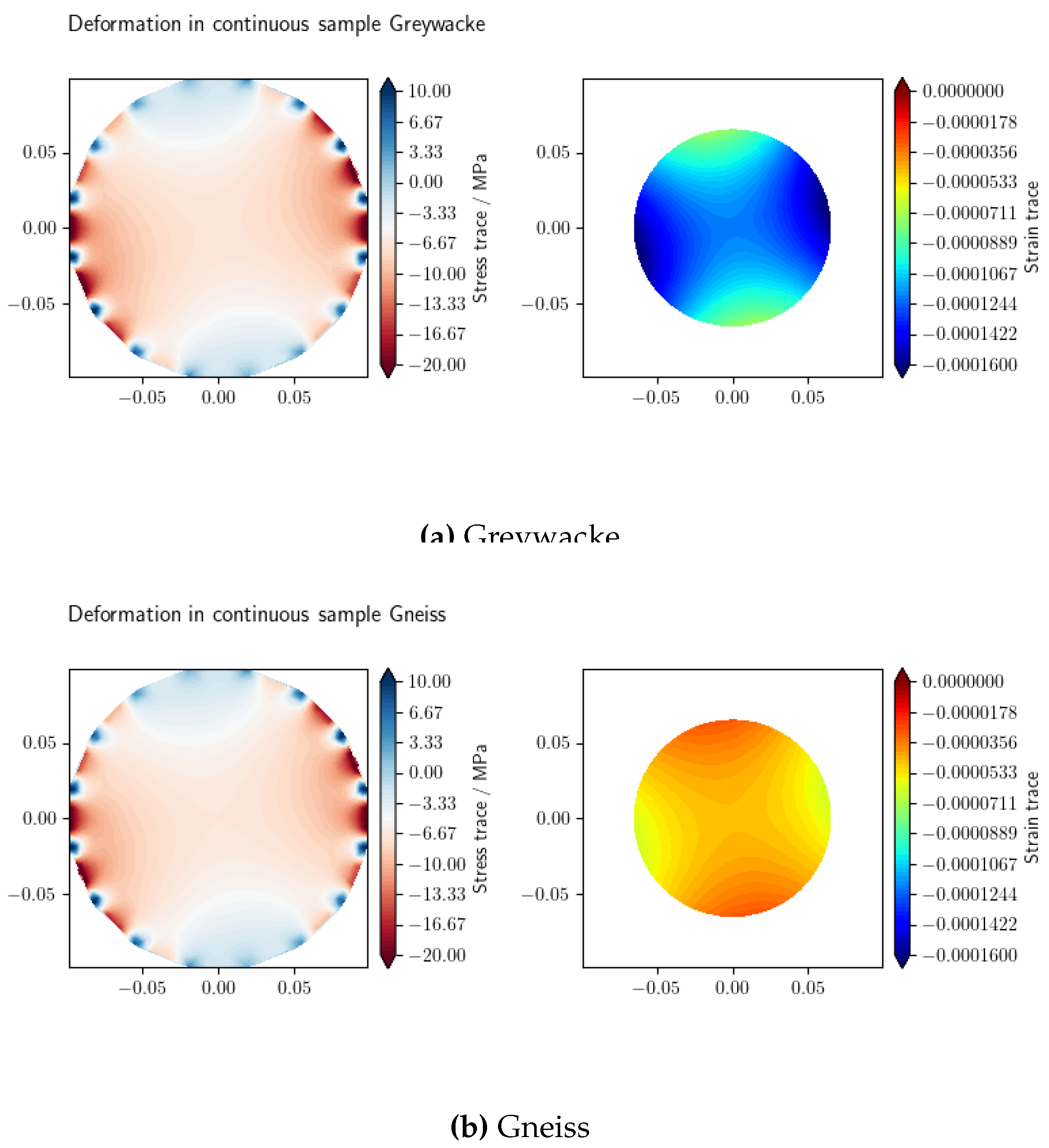
Figure 6.
/: Volumetric strain versus angle for an intact sample, under Load A (Table 1) at the final time (LIE-FEM & VPF-FEM).
Figure 6.
/: Volumetric strain versus angle for an intact sample, under Load A (Table 1) at the final time (LIE-FEM & VPF-FEM).
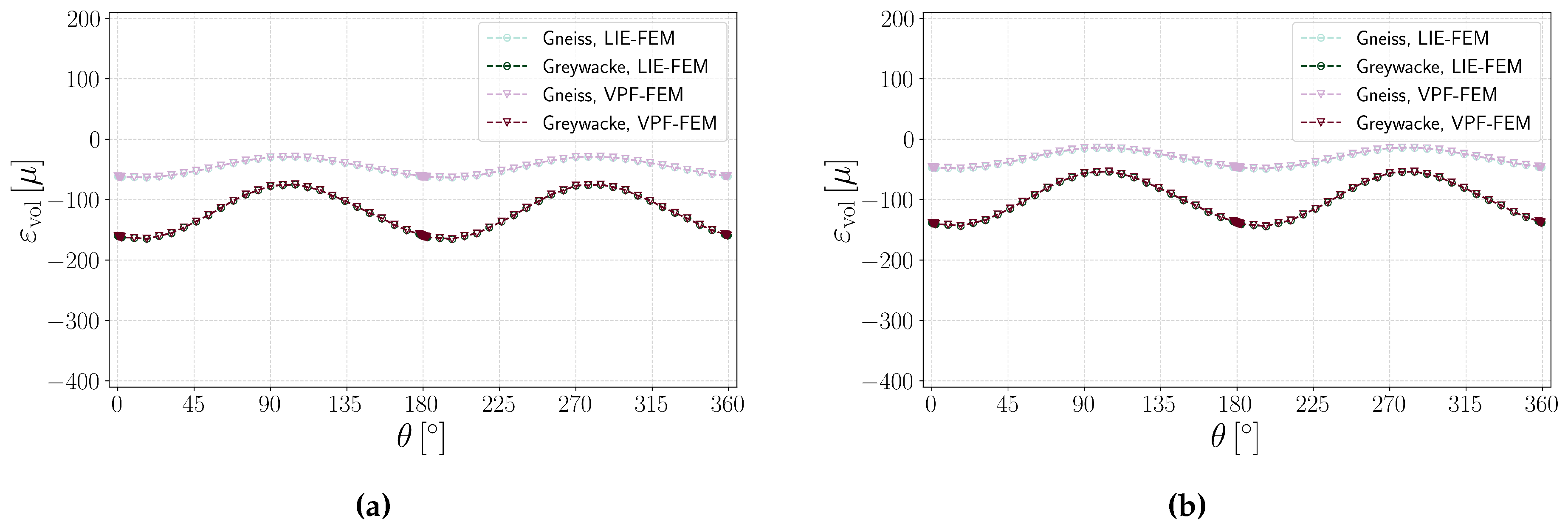
Figure 7.
: Pressure, trace of effective stress, and volumetric strain profiles of the Greywacke sample for the test under Load A at the final time (LIE-FEM).
Figure 7.
: Pressure, trace of effective stress, and volumetric strain profiles of the Greywacke sample for the test under Load A at the final time (LIE-FEM).
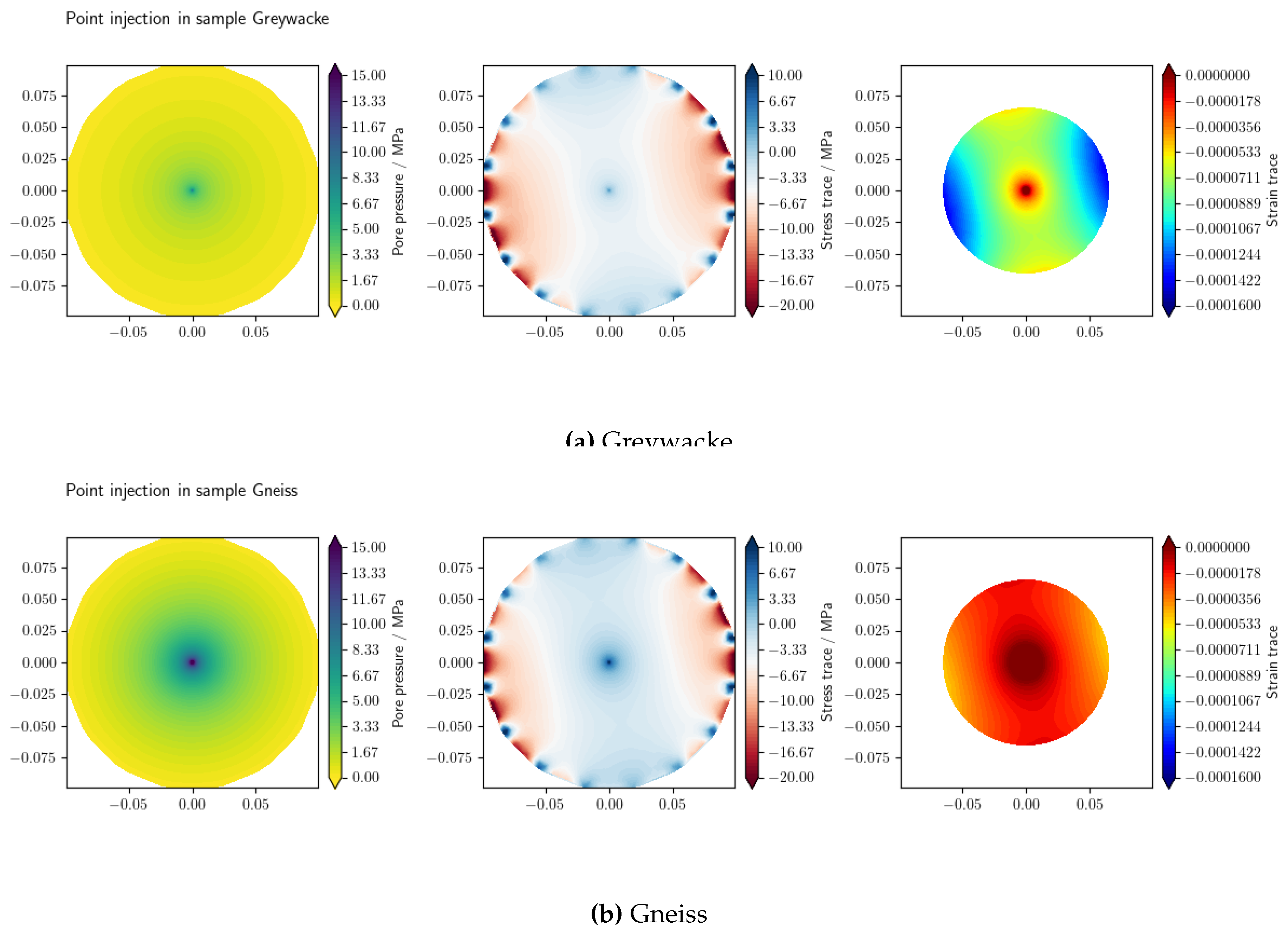
Figure 8.
: Trace of effective stress and volumetric strain profiles of the Greywacke sample for the test under Load B at the final time (LIE-FEM & VPF-FEM).
Figure 8.
: Trace of effective stress and volumetric strain profiles of the Greywacke sample for the test under Load B at the final time (LIE-FEM & VPF-FEM).
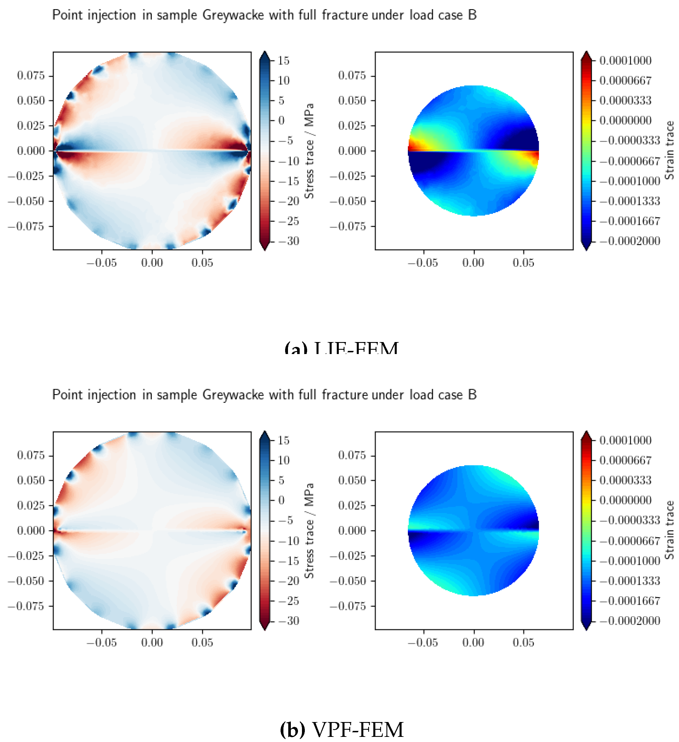
Figure 11.
: Pressure, trace of effective stress, and volumetric strain profiles of the Greywacke sample for the test under Load B at the final time (LIE-FEM & VPF-FEM).
Figure 11.
: Pressure, trace of effective stress, and volumetric strain profiles of the Greywacke sample for the test under Load B at the final time (LIE-FEM & VPF-FEM).
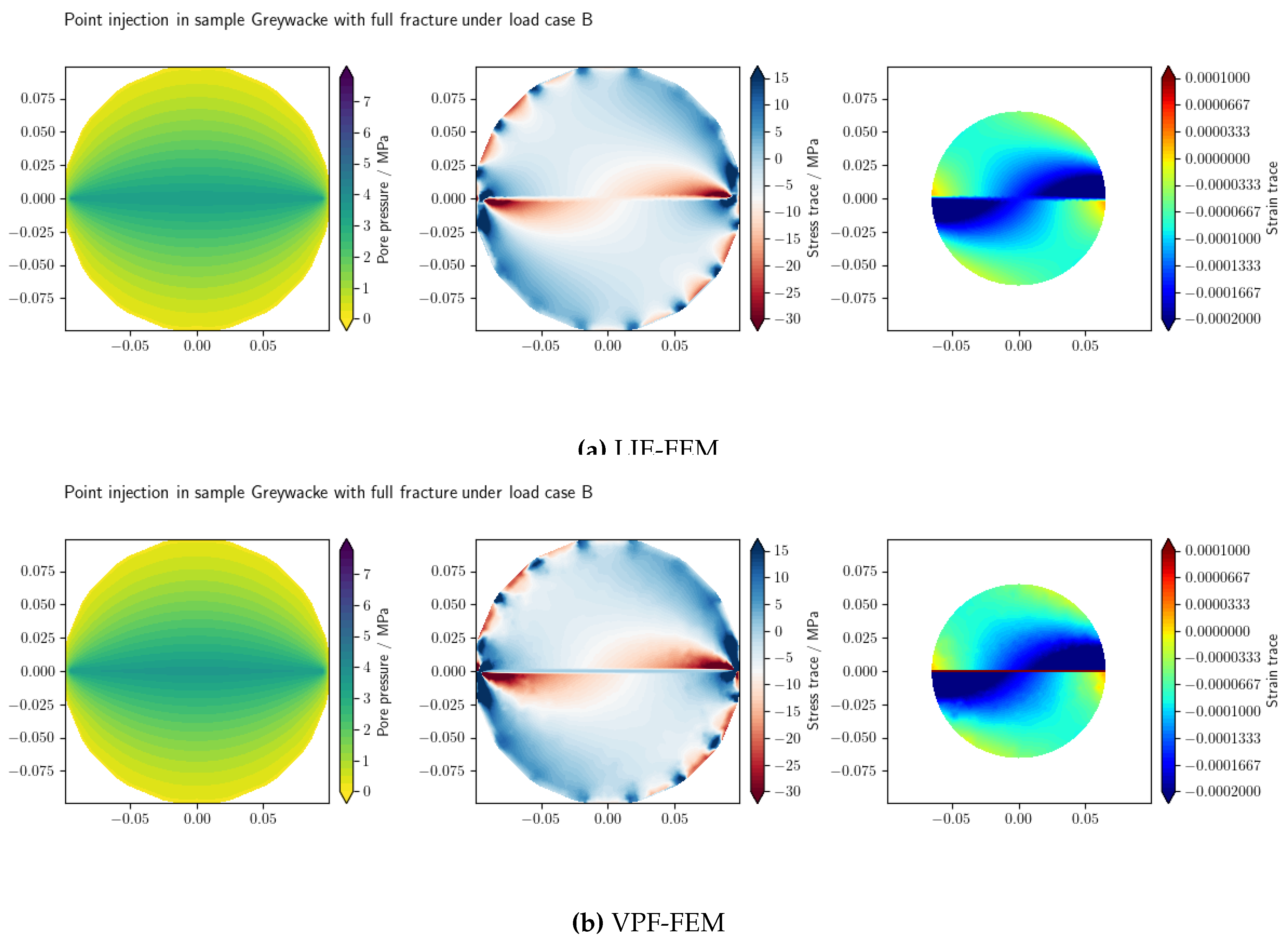
Figure 15.
: Phase field and pressure profiles of the Greywacke sample for tests at s after starting of fluid injection.
Figure 15.
: Phase field and pressure profiles of the Greywacke sample for tests at s after starting of fluid injection.
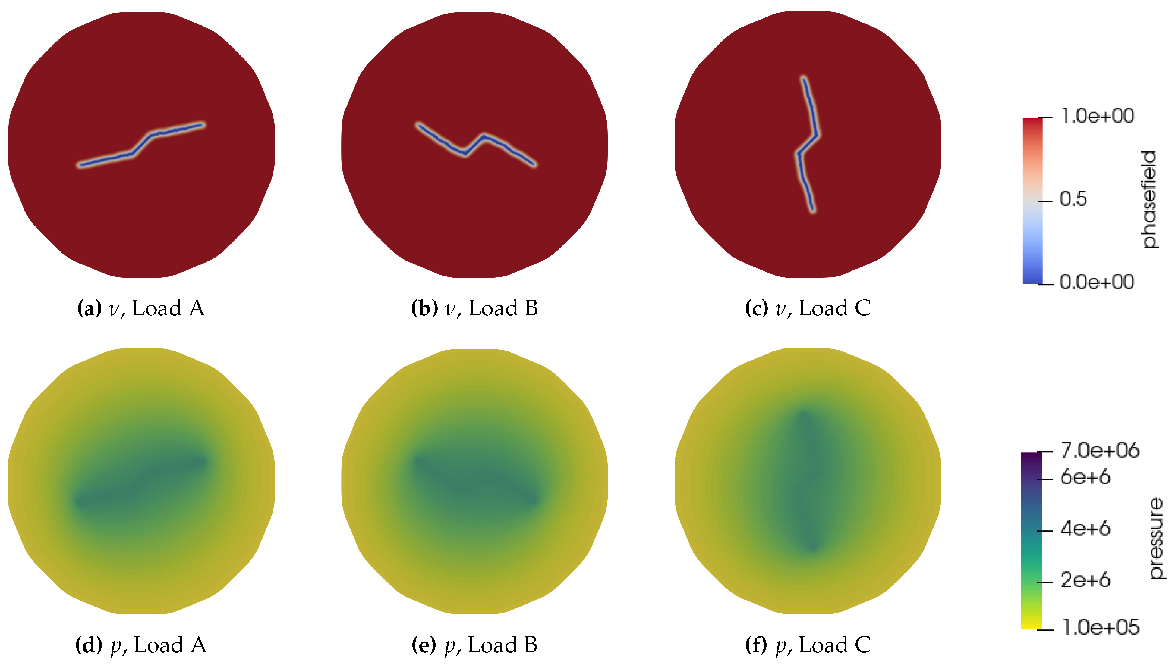
Figure 16.
: Phase field and pressure profiles of the Greywacke sample for tests at s after starting of fluid injection.
Figure 16.
: Phase field and pressure profiles of the Greywacke sample for tests at s after starting of fluid injection.
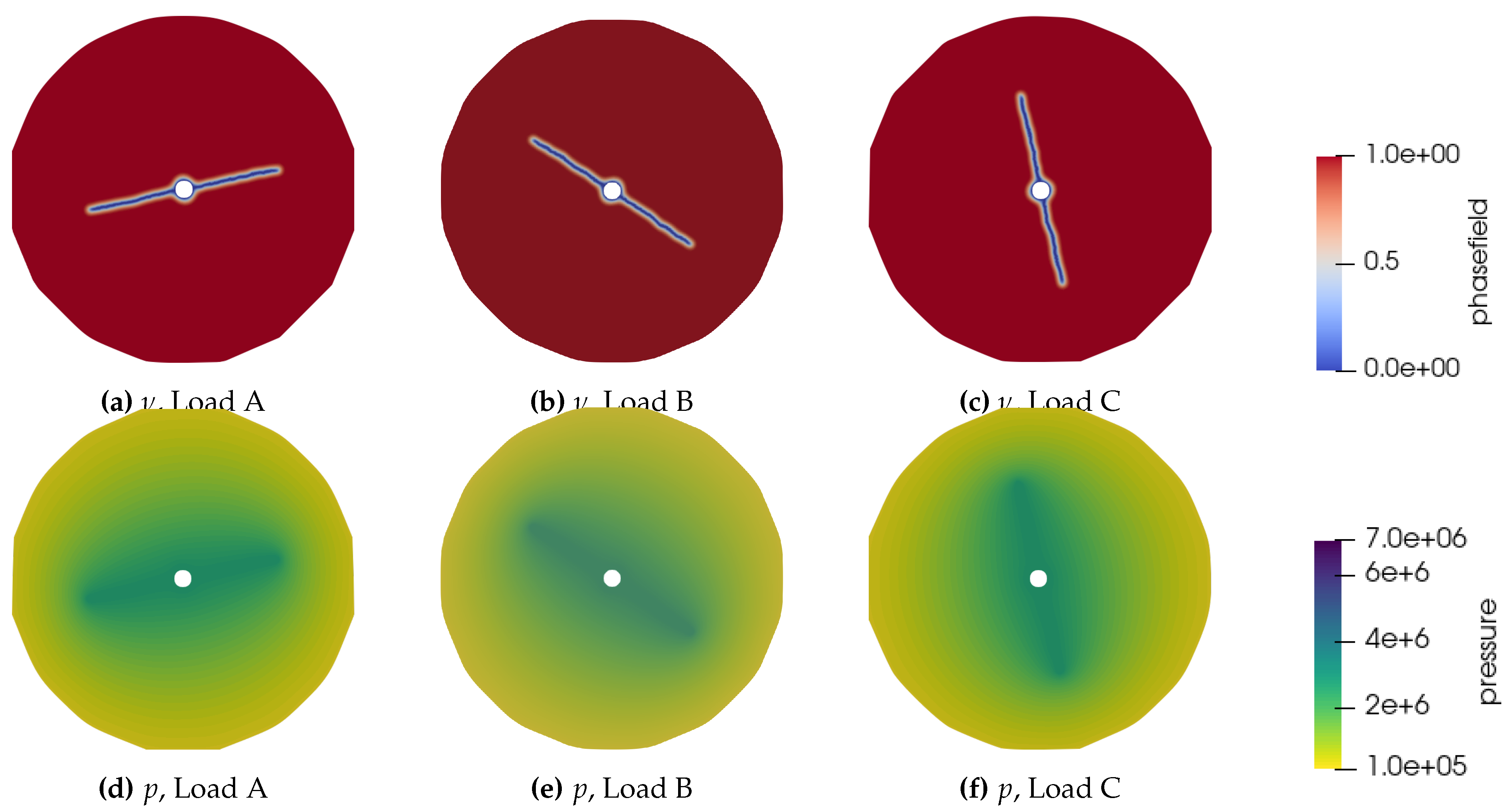
Figure 17.
: Pressure and trace of stress profiles (a) at an early stage after load application and (b) at equilibrium (when pressure reaches the initial value), before injection starts, under load A (LIE-FEM). At the early stage after load application, a high pressure is observed, which should be allowed to dissipate to reach equilibrium.

Figure 18.
: Mesh study for VPF-FEM (with Volumetric-Deviatoric strain energy decomposition) and comparison with LIE-FEM: (a) Volumetric strain on a probe circle at a radius of 0.065 m, and (b) Von Mises stress and (c) strain along a vertical line perpendicular to the fracture at .
Figure 18.
: Mesh study for VPF-FEM (with Volumetric-Deviatoric strain energy decomposition) and comparison with LIE-FEM: (a) Volumetric strain on a probe circle at a radius of 0.065 m, and (b) Von Mises stress and (c) strain along a vertical line perpendicular to the fracture at .
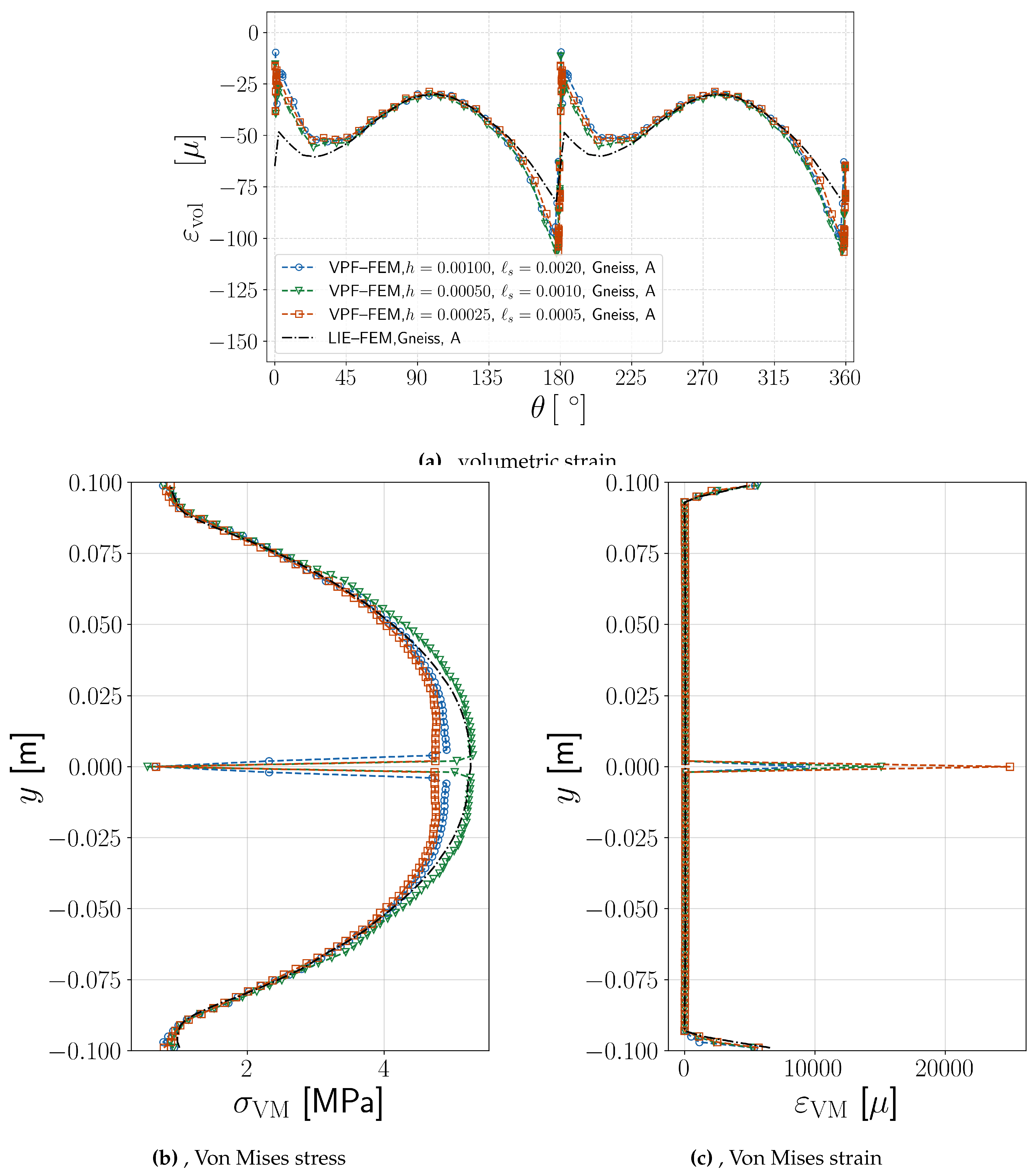
Figure 19.
: Strain energy decomposition for VPF-FEM and comparison with LIE-FEM: (a) Volumetric strain on a probe circle at a radius of 0.065 m, and (b) Von Mises stress and (c) strain along a vertical line perpendicular to the fracture at .
Figure 19.
: Strain energy decomposition for VPF-FEM and comparison with LIE-FEM: (a) Volumetric strain on a probe circle at a radius of 0.065 m, and (b) Von Mises stress and (c) strain along a vertical line perpendicular to the fracture at .
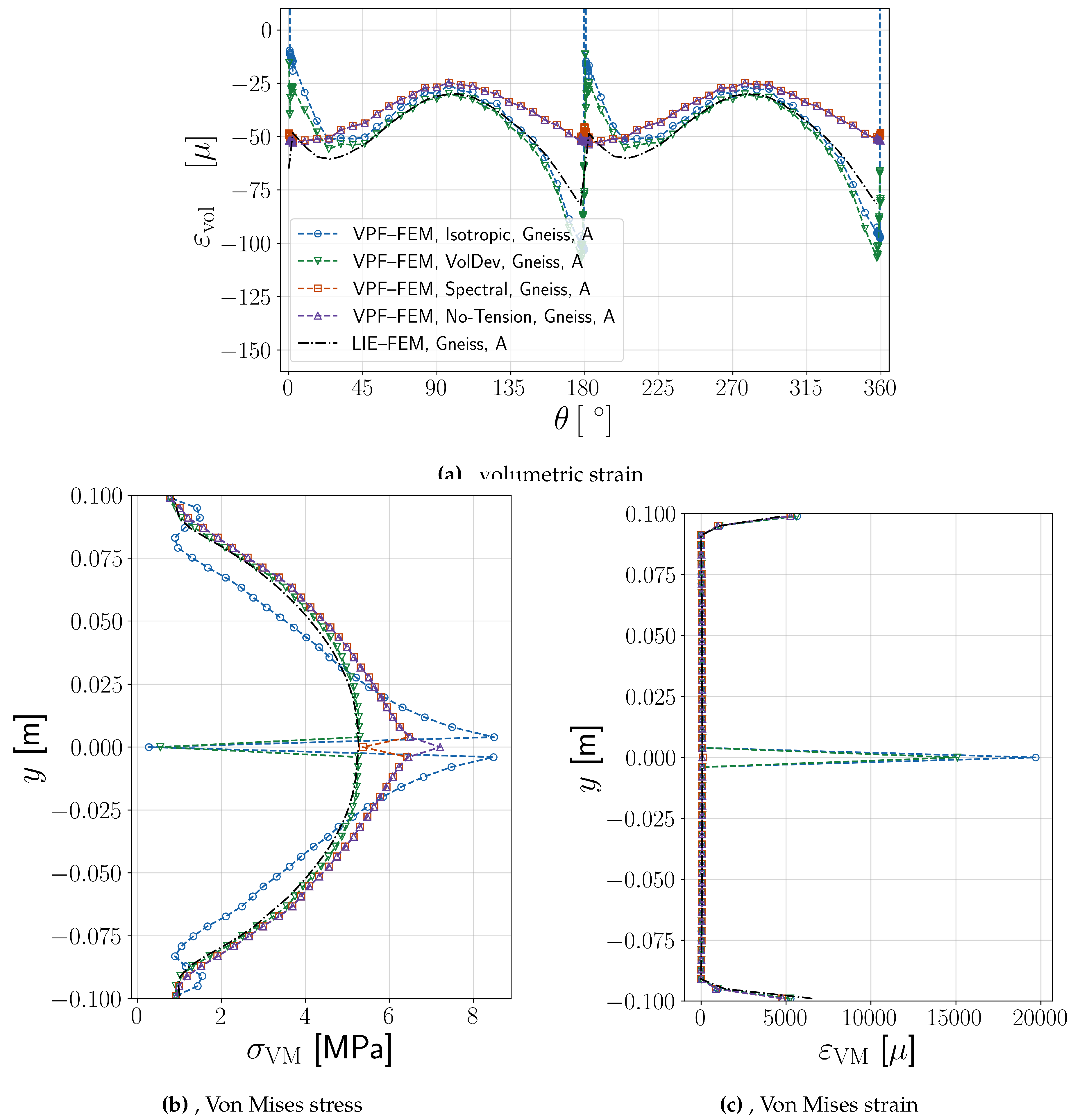
Figure 21.
: Sensitivity analysis of the effect of fracture stiffness ( and ) in LIE-FEM and comparison with VPF-FEM: Volumetric strain on a probe circle with a radius of 0.065 m
Figure 21.
: Sensitivity analysis of the effect of fracture stiffness ( and ) in LIE-FEM and comparison with VPF-FEM: Volumetric strain on a probe circle with a radius of 0.065 m
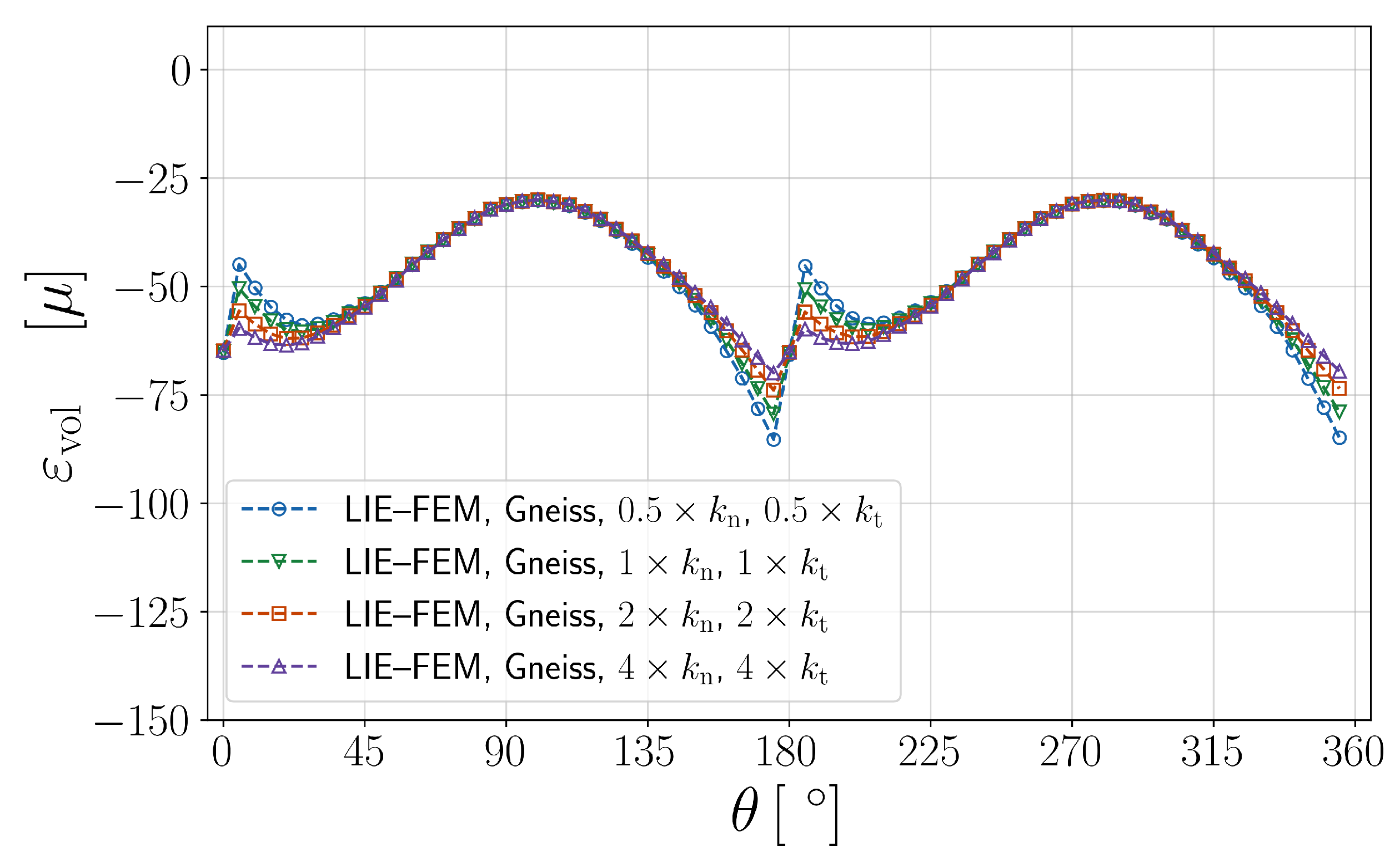
Figure 22.
: (a)&(c) show fracture width profiles under varying loading conditions across different materials. (b)&(d) show the average permeability corresponding to each loading condition across different materials.
Figure 22.
: (a)&(c) show fracture width profiles under varying loading conditions across different materials. (b)&(d) show the average permeability corresponding to each loading condition across different materials.
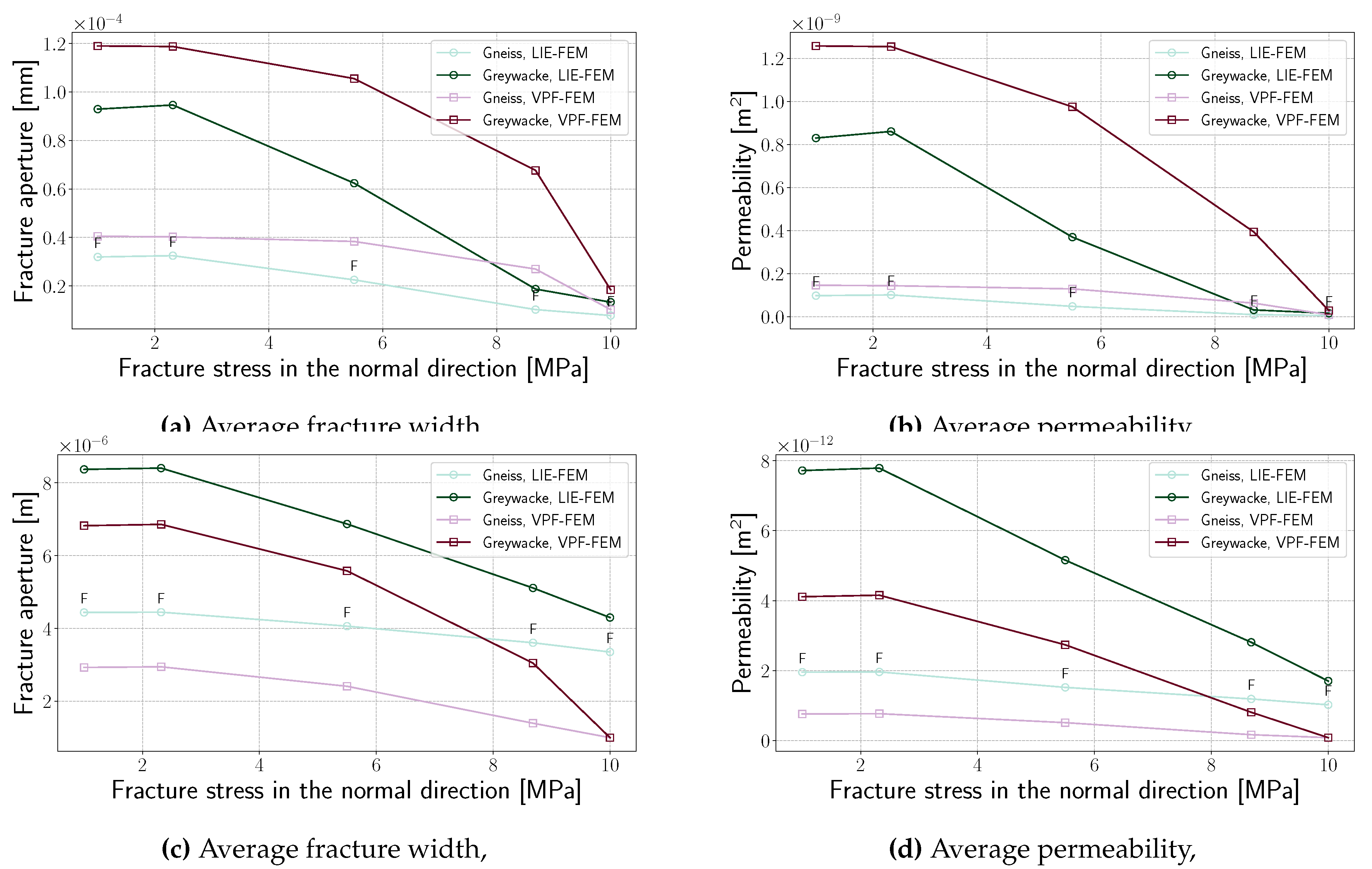
Figure 23.
Pressure evolution in the sample centre during fracture propagation (VPF simulations).
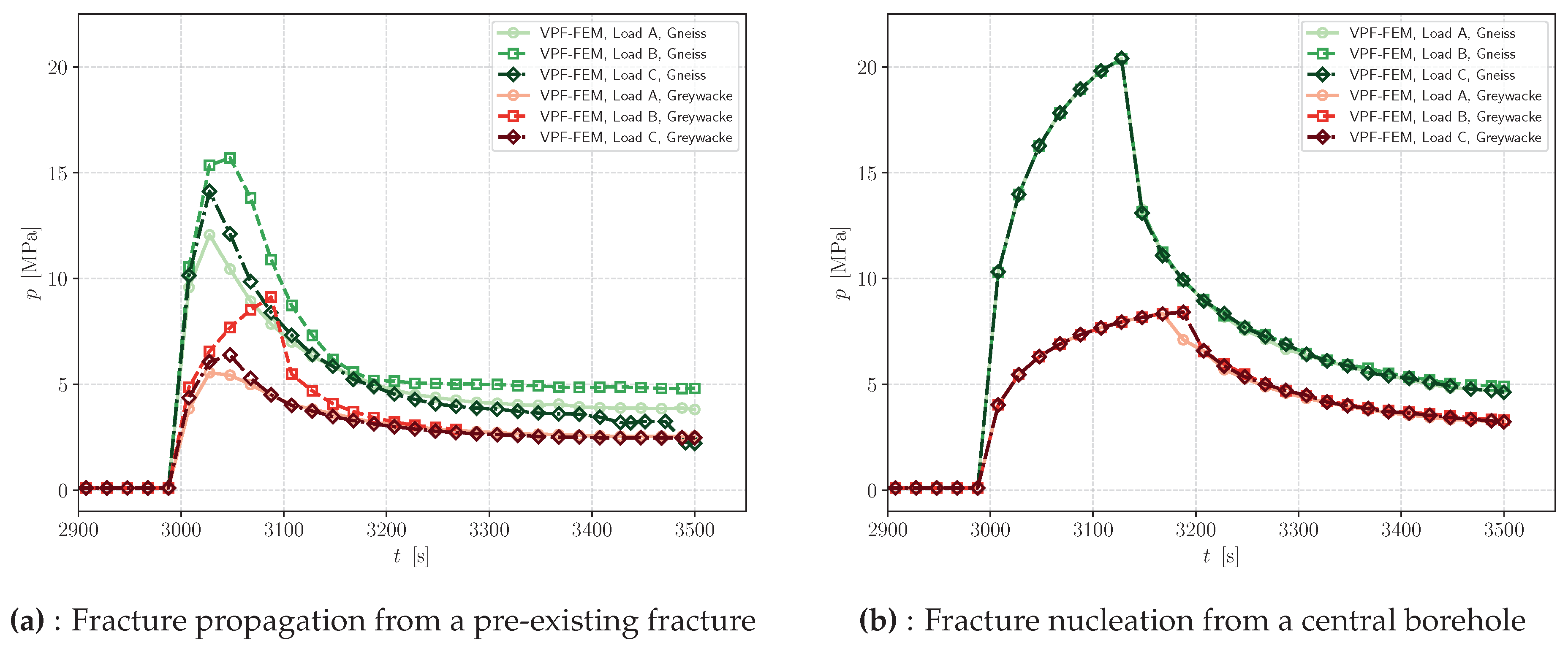

Table 1.
Overview of material properties for the GREAT cell samples
| Parameter | Unit | Material | |||
| Containing Sheath | Greywacke | Gneiss (Freiberg) | |||
| [25] | [25] | [23] | |||
| Young’s modulus, E | GPa | 0.1 | 26.85 | 83.9 | |
| Poisson’s ratio, | - | 0.4 | 0.27 | 0.21 | |
| Tensile strength | MPa | - | 17.01-16.67 | 16.8 | |
| Permeability, | m2 | 10−19 | 2.58 × 10⁻¹⁹ | 10−19 | |
| Solid density, | kg/m3 | 1200 | 2650 | 2750 | |
| Porosity, | - | - | 0.005 | 0.001 | |
| Biot coefficient, | - | 0.0 | 0.8 | 0.6 | |
| VPF–FEM | Fracture energy, | N/m | 0.1 | 30 | 50 |
| LIE–FEM | Normal stiffness, | GPa/m | - | 100.0 | 200.0 |
| Tangential stiffness, | GPa/m | - | 50.0 | 100.0 | |
Table 2.
Fluid Properties
| Properties | Values | Unit |
|---|---|---|
| Fluid density, | kg/m3 | |
| Viscosity, | Pa·s | |
| Fluid compressibility, | Pa−1 |
Table 3.
Load conditions for , , and simulations
| Marker | Angle PEE1 to | PEE’s | |||||||
| 1 & 1a | 2 & 2a | 3 & 3a | 4 & 4a | 5 & 5a | 6 & 6a | 7 & 7a | 8 & 8a | ||
| A | 0° | 10.0 | 6.64 | 4.46 | 1.17 | 1.0 | 3.82 | 7.80 | 9.95 |
| E | 22.5° | 9.95 | 10.0 | 6.64 | 4.46 | 1.17 | 1.0 | 3.82 | 7.80 |
| B | 45.0° | 7.80 | 9.95 | 10.0 | 6.64 | 4.46 | 1.17 | 1.0 | 3.82 |
| F | 67.5° | 3.82 | 7.80 | 9.95 | 10.0 | 6.64 | 4.46 | 1.17 | 1.0 |
| C | 90° | 1.0 | 3.82 | 7.80 | 9.95 | 10.0 | 6.64 | 4.46 | 1.17 |
DSS’s: average of loads of adjacent PEE’s. The loads are given in MPa.
Disclaimer/Publisher’s Note: The statements, opinions and data contained in all publications are solely those of the individual author(s) and contributor(s) and not of MDPI and/or the editor(s). MDPI and/or the editor(s) disclaim responsibility for any injury to people or property resulting from any ideas, methods, instructions or products referred to in the content. |
© 2025 by the authors. Licensee MDPI, Basel, Switzerland. This article is an open access article distributed under the terms and conditions of the Creative Commons Attribution (CC BY) license (http://creativecommons.org/licenses/by/4.0/).
Copyright: This open access article is published under a Creative Commons CC BY 4.0 license, which permit the free download, distribution, and reuse, provided that the author and preprint are cited in any reuse.


