
Submitted:
20 March 2025
Posted:
21 March 2025
You are already at the latest version
Abstract
We review simulations of polymeric fluids that report mean-square displacements g(t) of polymer beads, segments, and chains. By means of careful numerical analysis, but contrary to some models of polymer dynamics, we show that hypothesized power-law regimes g(t)∼t^α are almost never present. In most but not quite all cases plots of log(g(t)) against log(t) show smooth curves whose slopes vary continuously with time. We infer that models that predict power-law regimes for g(t) are invalid for polymer melts.
Keywords:
polymer dynamics
; mean-square displacement
; polymer melt
; polymer solution
; computer simulation
; scaling behavior
; scaling exponents
; power-law behavior
1. Introduction
In this paper, we consider a few aspects of polymer motion in simulated bead-bond polymer melts. Our interest is the time-dependent mean-square displacement of individual beads, of polymer centers of mass, and of polymer beads with respect to the center of mass of their polymer chain. We advance via a review of representative papers from the literature, applying a quantitative approach based on standard numerical methods. A short letter demonstrating the approach has been published previously [1].
The behaviors of the mean-square displacements are predicted by tube-reptation-scaling models of polymer dynamics [2,3]. For long polymers in a melt, the tube model proposes that the polymer chains surrounding a chain of interest form a transient pseudolattice that restricts the chain of interest’s lateral motions. The transient pseudolattice is described as a tube, an irregular curving barrier having statistical diameter a and contour length L, within which the chain of interest is momentarily confined. According to the tube model, the polymer chain of interest is said to be constrained to move more-or-less parallel to its tube.
For long polymer molecules, the tube model introduces three characteristic times. The hypothesized times are claimed to separate four characteristic time scales for polymer motion. At times shorter than an entanglement time , beads are said not to have encountered the walls of the tube, so bead motions are claimed to be described by the simple Rouse model. At times between and a later time , Rouse relaxations continue, but are perturbed by the tube walls until they completely relax at a time . , the Rouse time, is the time scale on which the polymer’s longest-lived Rouse mode would relax, if the polymer’s dynamics were described by the Rouse model for a bead-spring chain [4]. is defined in terms of other chain properties as
Here is a bead drag coefficient, N is the number of beads in the polymer, is the polymer’s mean-square radius of gyration, is Boltzmann’s constant, and T is the absolute temperature.
Between and a disengagement time , the polymer diffuses back and forth along the length of its tube. The tube’s ends fray and disappear whenever the polymer backs away from them. Over times greater than , the polymer is no longer confined by the tube and instead performs simple diffusion. The tube model indicates that it does not describe the motions of short chains. Instead, for short chains there are only two time regimes, as described by the Rouse model, the time regimes being separated by the time .
Tube models of polymer dynamics make a series of predictions that are accessible to simulational tests. Of particular interest are predictions of mean-square displacements, including displacements of individual beads and displacements of the chain center of mass. The atomic mean-square displacement for a chain is described by
Here and are times. The sum may be over the positions of all N beads of a chain, or over the positions of a subgroup of n beads in a longer chain. Motions of a subgroup centered on the chain center are typically considered. The average includes averages over all chains and over all values of the initial time .
The center-of-mass mean-square displacement is
where is the position of a chain center-of-mass at time t, the average being over all chains and all initial times . Center-of-mass displacements have been reported using the center of mass of all beads in a chain or separately by using the center of mass of the central beads of a chain.
The mean-square displacement of monomer beads relative to their polymer’s center of mass is described by
where n is the number of beads in a chain.
When need be, we refer to the mean-square displacement functions collectively as the .
The Rouse and tube models predict the time dependences of these mean-square displacements, the predictions all having the form . The exponent depends on the polymer chain length and the time scale over which the time dependence is being described.
For melts of short chains the tube model predicts that polymers have the properties predicted by the Rouse model, namely
At times , chain motions in a polymer melt are said to be described by the relaxation of pure Rouse modes, leading to for and for . At longer times , is predicted both for and for .
For long chains, the tube model predicts for single-bead mean-square displacements that
and have the same behavior until , following which reaches a plateau at .
For long chains, the tube model predicts for center-of-mass mean-square displacements that
The regime for long chains during is often viewed as a signature that the tube model is correct. However, as noted by Puetz, et al. [5], in the same time regime the Schweizer mode-coupling model [6,7] predicts a very similar time dependence for , even though Schweizer’s model gives an entirely different description of bead motion. Similarly, in the following regime, is predicted by the tube model to be proportional to , while the Schweizer model predicts . From , it may therefore be difficult to distinguish between the tube and Schweizer models.
A few authors calculate the full distribution of displacements r at each time t. When is non-Gaussian, a non-Gaussianity parameter has been introduced. is defined as
If , interpreting as supplying a (time-dependent) diffusion coefficient is invalid, because particle motion does not have the Gaussian displacement distribution required by Doob’s theorem [8] if the particle motion is Brownian diffusion. In addition, if , it would be incorrect to relate to the dynamic structure factor by using a Gaussian approximation , because this form is only correct if particle displacements have a Gaussian distribution of values at all times [9]. If is not a Gaussian, the Gaussian approximation for may be incorrect even as an order-of-magnitude approximation.
Here we consider simulated determinations of polymer mean-square displacements and what they say about the validity of the deGennes-Doi-Edwards tube model. Our focus is careful numerical study of the time-dependent mean-square displacements, comparing with predictions, covering chains of all lengths, that there are regimes in which the mean-square displacements , , and have power-law dependences on time. Our interest here is less what exponents are found and more whether or not a power-law dependence is present at all.
How might power-law dependences be demonstrated? In the simplest case, if there were a power-law dependence , a graph of against would reveal a straight line having slope . Multiple straight-line regions might well be separated by smooth curves marking crossover regimes. Here we replace this crude graphical approach with a systematic quantitative method.
This paper represents an extension of our prior reviews on the phenomenology of the dynamics of polymeric liquids. In our prior volume Phenomenology of Polymer Solution Dynamics [10], we considered the concentration, molecular weight, and time dependences of polymer solution properties, including centrifugation, electrophoresis, polarized and depolarized light scattering spectroscopy, solvent diffusion, segmental relaxation, dielectric relaxation, mutual diffusion, probe diffusion, viscosity, viscoelasticity, non-linear viscoelastic behavior, and outcomes of the same techniques as applied to solutions of spherical colloids. A systematic comparison of experiments on polymer solutions with theoretical models found that hydrodynamic scaling models [11] worked well, but reptation-scaling forms [2], e.g., for the self-diffusion coefficient, and being constants, were uniformly inconsistent with experiment. At that time, we were challenged to discuss whether our results applied to melts but were not prepared to do so. This paper is part of a series now responding to that challenge. In a recent paper [12], we extended our reviews to simulations of polymer melts, notably the behavior of the nominal Rouse modes, finding that Rouse mode amplitudes of polymers in melts do not have the properties predicted by Rouse. Here we continue this study, turning to the behavior of the mean-square displacements as found in polymer simulations.
The remainder of this paper has three sections. The next Section presents our quantitative method for analyzing to determine actual time dependences. We have previously presented tests of the method against representative data. [1]. The following Section applies these quantitative methods to results from the simulation literature. A final Section discusses what has been found. The verisimilitude of our analysis arises from the graphical presentations of our numerical analyses, so the Supplemental Figures present at full scale all of our results.
2. Methods
In this paper, we re-analyze literature reports of of simulated polymeric systems. Most measurements in the literature are reported as smooth curves, not as the discrete points normally generated by molecular dynamics simulations. Digitization of reported determinations was accomplished using UN-SCAN-IT [13] under manual control. The significant obstacle, at least in some papers, was that the authors conserved space by plotting multiple sets of results on a single graph. In some cases data points were sufficiently overlapped that determinations of became impossible.
We advance by curve fitting. Identifying and , we fit to polynomials
Here the are the fitting parameters, to be obtained from linear-least-mean-squares analysis, and N is the truncation limit, the largest value of n in a given fit. What value of N is appropriate? We repeatedly fit measurements to equation 17 with progressively increasing values of N. The mean-square difference between the fitted curve and the measurements was obtained. We consistently found that there was an upper limit on N above which further increases in N gave at most a very limited reduction in the mean-square difference between the simulational measurements and eq. 17. was generally used as the cutoff in the studies here. As seen below and in teh Supplemental Material, our fitted polynomials accurately follow simulational determinations of the , with no indication of a need to fit different time regimes with distinct polynomials employing different sets of .
In our analysis,
is the logarithmic derivative of our polynomial. For each t, gives the instantaneous value of in a local-in-time scaling law . If power-law behavior were present in some time regime, within that regime would be constant up to noise. To test for constancy, we also calculated the second logarithmic derivative
In general, and both depend on t. In a power-law regime, one expects over an extended range of times. Noise in the simulation, the digitization process, and the numerical fitting steps will lead to noise in , so in a power-law regime will in general not be exactly zero. will also be found over a narrow range of times wherever has a maximum, a minimum, or a saddle point, but these cases are readily distinguished from power-law behavior.
Our analytical approach appears to be more sophisticated than has oft-times been applied to identify power-law regimes. This observation is not meant as a criticism of earlier work. The earlier processes were entirely adequate for the needs of their users. We only claim that our more powerful mathematical technique reveals hitherto obscure features that were actually present in the original studies. In particular, we do not attempt to force the interpretation that , i.e., that actually has a linear dependence on over some range of times. We instead determine the dependence of on , and inquire as to whether that dependence is linear in , as would be the case if .
Our procedure creates smooth curves that, at least in the studies discussed here, always visibly pass within noise through the measured . The logarithmic derivative of the fitted function provides, for each time, the local value of the exponent, as could in principle be obtained by a fit of a power law to over a narrow range of . As a practical matter, we found that direct fits of to over short ranges in time were quite noisy, so we tried but did not pursue examining as obtained from a multitude of local fits. In contrast, logarithmic derivatives of equation 17 are nearly noiseless. This distinction between our approach and local fits is the well-known issue that, while numerical integration tends to suppress noise, numerical derivatives tend to amplify noise. We emphasize that polynomial fits are interpolants, not extrapolants. They fill in the space between measured points, but are unreliable as predictors outside of the range of times over which the fit was made.
3. Analysis
In this Section, we use our numerical analysis approach to consider as reported by a series of authors. Strong conclusions, as will be presented here, need strong support. We therefore include eighty determinations of . While we could have selected from these an exemplary set of a few systems, this path would have led to suggestions that we had cherry-picked data to support our conclusions. On the other hand, there is a certain uniformity in the time dependences of the and of . In almost every case: increases monotonically, on a log-log plot more rapidly at early and late times and less rapidly at intermediate times. With increasing time, the first logarithmic derivative decreases more or less smoothly to a minimum, corresponding to an inflection point of , and then increases more or less smoothly again. In a very few cases, we find that has a single extended region in which it is constant, corresponding to a power-law dependence of on t. In no system do we observe more then one power-law regime for , other than at the short- or long-time limits.
Behbahani and Schmid [14] report simulations of a Grest-Kremer bead-spring polymer model [15]. Beads had mass m and a purely repulsive Weeks-Chandler-Anderson potential [16] with length scale and energy . Bead-bead bonds were represented with a FENE (Finite Extensible Nonlinear Elastic) potential [17]. Studies were made for polymers having between 5 and 1000 beads with a minimum of 192 chains in a simulation box. Time was measured in natural units , simulations being extended out to to depending on chain lengths. Behbahani and Schmid note a series of estimates of the entanglement length, one group of estimates in a cluster near 50 beads and another in a cluster of 80 or a few more beads. The authors use the former number to estimate that their thousand-bead polymer has on average some 20 entanglements. The estimated distance between entanglements, which was identified as the tube diameter a, was estimated to be approximately . From their simulations, Behbahani and Schmid calculate the mean-square bead displacements, the mean-square displacements of the central beads, the mean-square center-of-mass displacements, the time dependence of the polymer end-to-end vector, the single-chain dynamic structure factor, the stress relaxation modulus, and the zero-shear viscosity.
We first consider single-bead motions. Figure 1 and Figure 2 show Behbahani and Schmid’s determinations of mean-square single bead displacements in their systems, and our fits of to a power series in . We used fits to eighth-order polynomials, except thatin one system (the 400-bead polymer, Figure 2c) the eighth-order fit to was not entirely satisfactory, so a tenth-order fit was used instead. What features are revealed by ? For the 10-bead chains, has a minimum, and correspondingly has an inflection point near . For longer chains, there appear to be two features that emerge and separate with increasing chain length. The 1000-bead chains show these clearly. First, has a minimum, so has an inflection point. Second, at shorter times before reaching its minimum, has an extended region in which it decreases linearly with (and, correspondingly, ). For shorter chains, the near-linear region acquires weak distortions from linearity. Finally, for the 100- and 50-bead polymers, the linear region and the minimum in blend into each other, so that one could reasonably describe the region near the apparent inflection point as showing power-law behavior. The value of at its minimum, the slope of at the inflection point, decreases with increasing chain length, from 0.65 for the 10-bead chains to 0.31 for the 1000-bead chains. Over the same series of simulations, the location of the minimum increases, from for the 10-bead chains to for the 1000-bead chains. Table 1 shows the full dependence of on chain length.
Close to the shortest and longest times studied, we sometimes see an additional feature in the time dependence of . As seen in Figure 1a,d and Figure 2a,c, the feature is a local maximum in , in these figures located just before the largest times studied. We note the feature, but are not certain whether it is real or is a consequence of the operation of our polynomial fitting process near end points.
Behbahani and Schmid also report as calculated using only the displacements of the central beads of the polymer. It is generally stated that polymer end beads are more mobile than beads near the center, for reasons not arising from core parts of the reptation-tube model, so a study of central beads may well be a better test of that model. Figure 3 shows their results for the 1000-bead polymer, and our fit to their results. for central beads indeed has an inflection point (a minimum in ) for , this being the slope predicted by the reptation-tube theory as a central outcome of the model. Those authors justifiably propose that they have observe the predicted region emerging from surrounding transition regions. One notes, however, that the minimum of progressively decreases with increasing polymer chain length, so a needed experiment would study somewhat longer polymers, say 1300 or 1500 beads, to determine whether for longer chains the minimum in remains near , or whether with increasing chain length the minimum in continues to decrease, in which case the observed 0.25 would be a coincidence arising from a fortunate choice of chain length. As with , at times shorter than that at which the inflection point is seen, there is an extended region in which decreases linearly with . The physical interpretation of this observation is unclear.
We finally consider Behbahani and Schmid’s determinations of center-of-mass motions. Figure 4 and Figure 5 show their measurements of mean-square center-of-mass displacements . Once again, the time dependence of shows that for each polymer length has an inflection point. The slope at the inflection point decreases with increasing polymer length, from for the 10-bead polymers to for the 1000-bead polymers. With increasing chain length, the time at which the inflection point is found also increases, from for the 10-bead polymer to for the 1000-bead polymer. At times before the inflection point, has distinct short- and long-chain behaviors. For the shorter chains, beads per chain, decreases smoothly with decreasing slope until it reaches the inflection point. For the longer chains, 200 beads or more per chain, acquires a shoulder covering 2-3 decades in time before it reaches its minimum.
Chang and Yethiraj [18] explore a polymer model in which polymer molecules may or may not be allowed to pass through each other, depending on the value of a single parameter. They model polymers as chains of hard spheres having diameter coupled by bonds whose lengths can fluctuate freely over a range of lengths . Beads interact via elastic collisions. In different simulations, chains had lengths N between 8 and 512 beads at bead volume fractions of 0.3 or 0.4, with ranging from 0.05 to 0.9. Chain crossings are blocked for , marginally possible for , and become more frequent as is further increased. They calculated a diffusion coefficient D for the chains, finding that was approximately constant for but decreased at larger N, and inferred that marked the onset of entanglement. Static chain properties, the pair correlation function and the static structure factor, are nearly independent of . Chain dynamic properties are sensitive to the chain crossing parameter, showing one behavior for and a different behavior for . In particular, for long chains the chain self-diffusion coefficient scales as for large and as for small .
Of particular interest here, Chang and Yethiraj calculated the mean-square displacements of the chain centers of mass and the chain central monomers for , , and . The 0.4 and 0.45 results are nearly indistinguishable. These are the chain-nearly-non-crossing simulations, so we will consider only the simulation.
As seen in Figure 6, Chang and Yethiraj’s determinations of are all described well by polynomial curves. The first derivatives are equally well-behaved. Beginning with the center-of-mass displacement measurements as described by : As seen in Figure 6a, for , increases smoothly from approximately 0.7 to 0.8 with increasing t, and at the largest t appears to increase to 0.9 or so. Figure 6b reveals for that earlier times is nearly constant, increasing by 0.03 over its near-constant range; at , increases progressively toward . From Figure 6c, for , at first increases rapidly, and then rises gradually from 0.8 to a plateau near 0.95.
Chang and Yethiraj also calculated for the central monomers of their chains. For , the corresponding lies in the range 0.35-0.40, except at the longest and shortest times reported, as seen in Figure 6d. Figure 6e gives results for , for which is consistently near 0.39. except at the two extrema, where it rises to 0.45 or 0.55. On increasing to 0.6, becomes larger, and increases smoothly from 0.45 to 0.5 over most of the observed time range, with a modest further increase to about 0.6 at the largest times studied.
Chang and Yethiraj propose that the power-law time regimes of the reptation-scaling model are seen in their central-bead results for , these results being shown in Figure 6d. In this figure we find that follows a smooth curve with a not-quite-constant slope in the range 0.35-0.4, the slope never decreasing to the 0.25 of the scaling model.
Tsalikis, et al. [19] report simulations of ring and linear polyethylene molecules in the melt. They examined monodisperse systems of chains having 120, 227, or 455 monomers, corresponding to molecular weights of 5330, 10,044, or 20,086 Da, which they refer to as the PEO-5K, PEO-10K, and PEO-20K melts. For their systems, they estimate . Simulations were carried out using Fischer’s united-atom force field [20,21]. For the PEO-20K melt, the simulation cell contained more than 50,000 united atoms. Tsalikis, et al., report detailed studies of static and dynamic properties of their polymers, including . Figure 7 shows from their Figure 13, our fits to their simulation data, and the corresponding first derivatives. The ring data correspond to mean-square displacements of all monomers, while the linear chain data are for the ’most central’ (their words) monomers. They terminated their measurements at the Rouse times for each system. At each molecular weight, the linear chain’s central monomers move more rapidly than the monomers of the corresponding ring. Tsalikis, et al., interpret their results on the PEO-5K and PEO-10K systems as showing as showing two distinct breaks in , the lower being near 2nS and the higher being at 150 or 490 nS.
Figure 7 shows Tsalikis, et al.,’s measurements of in their six systems. Points are their measurements as digitized here; the original measurements were reported as solid lines. In Figure 7a, the 120-bead linear molecules, the slope falls from 0.6 at 0.2 nS to 0.38 at 22 nS and then rises again to 0.8 at the longest time reported. is visibly a local minimum. Figure 7b shows the corresponding results for the 120-bead ring polymer. As a function of time has a minimum at 20 nS, very nearly the same time as for the linear polymer, but here is 0.44. At longer times, rises to 0.95, which does not appear to be a maximum. Figure 7c,d show the corresponding results for the 227-bead linear and ring polymers. In these two systems, has minima at 0.30 and 0.43, respectively. For the ring polymer, a case can be made that there is a region within which is nearly constant, namely is within 1% of its 0.43 minimum for nS. Figure 7e,f, for the 455-bead linear and ring polymers, somewhat repeat the behavior seen for the 227-bead polymers. For the linear 455-bead polymer, falls from 0.57 at 0.33 nS to a minimum of 0.2 near 450 nS and then rises steeply at later time delays. The 455-bead ring polymer, like its 227-bead ring counterpart, has an extended minimum between 70 and 250 nS with .
For each of the larger rings, we have therefore found a single power-law region, though not with the same exponent in the two cases. With increasing chain length, the time dependence of softens, but key characteristic features only change numerically. In describing their results, Tsalikis, et al., instead say that there are clear breaks in separating extended regions in which follows one power law or another. We do not see these multiple power-law regions in our analysis.
Takahashi, et al. [22], report extended simulations of a united-atom model for polyethylene. They used the TraPPE-UA model, including Lennard-Jones potentials between non-bonded atoms, rigid links using the LINCS algorithm, bond bending with a harmonic potential, and torsional potentials along the chain backbones. Chain molecular weights ranged from 423 to 2807 Da, with 150 to 1000 chains in a periodic box. They estimated or equivalently , implying that their chains were unentangled or slightly entangled, with at most 2-3 entanglements on a single chain. The mean-square displacement of the chain central bead was calculated as a function of time. From the time correlation function of the chain end-to-end vector, a nominal relaxation time was inferred. A transition in the molecular weight dependence of was observed near a molecular weight of 1000, with at smaller molecular weights and at larger molecular weights.
Figure 8 shows our digitization of their measurements of , our polynomial fits to those measurements, and the computed logarithmic first derivatives . Agreement between the measured values and the polynomial fits is uniformly excellent. Of particular interest is Figure 8b. At longer times pS, lies on a straight line having slope unity. Correspondingly, the plot of against time shows a straight horizontal line, confirming that shows power-law behavior with . This result confirms that our method does reveal power-law behavior when it occurs. At shorter times, the slope of in each of these systems has a local minimum, corresponding to having a shorter-time inflection point. The slope at the inflection point decreases with increasing polymer molecular weight, the slopes at the six minima in order of increasing polymer length being 0.73, 0.64, 0.60, 0.53, 0.46, and 0.44, respectively.
For the 2807 Da polymer, Takahashi, et al., note that the sequence of straight-line slopes from the reptation-scaling model approximately resembles the curving , except that the “…threshold values …”, the moments in time at which one transitions from one power law to the next, are “…unclear …” in the graph. We agree with their conclusion, namely that except at the longest time follows a smooth curve with no ’transitions’.
Peng, et al. [23] report simulations of dynamically asymmetric A-B blends as functions of chain lengths and concentrations. Under some conditions the A and B chains become immiscible. The authors studied both phase-separated systems and systems which do not phase separate over the duration of the simulations at the simulated temperature. Their polymer beads interact via a Lennard-Jones potential and, along each chain, a FENE potential. A and B chains all use the same Lennard-Jones and FENE parameters. The A chains were made stiffer by endowing them with a harmonic bond-bending potential and a torsional potential. B chains had a fixed length ; A chains had lengths in the range 3-100. Nominal entanglement lengths were given as 28-45 for the A chains and 85 for the B chains, so the B chains were not entangled and the A chains would at most have been weakly entangled. The simulation cells all contained approximately 40,000 beads, all having the same mass. Simulations calculated an extended series of dynamic properties including bead and center-of-mass mean square displacements, Rouse mode temporal autocorrelation functions, and deviations from a Gaussian distribution of displacements, as represented by the non-Gaussianity parameter of equation 16.
Figure 9 shows a representative sample of Peng, et al.’s determinations of the mean-square displacements of B beads in a pure-B melt and in A-B mixtures, both in phase-separated and phase-non-separated systems. The A beads, when present, were at a mole fraction of 0.1. The dependence of on the chain length of the A beads was very weak.
These are rather short polymers. In each system, at the shortest times approached 2.0. then declined rapidly to an inflection point, the minimum of being in the range 0.15-0.28 at times 2-2.5. then increased again to 0.55-0.59 in the four displayed systems. From the measurements, in these systems show: shorter-time asymptotic behavior, an inflection point at intermediate times, and near-power-law behavior at the longest times studied. There are no indications of additional power-law-regimes at intermediate times. Our finding of a long-time power-law regime is in quantitative agreement with the analysis of Peng, et al., [23] who report power laws with at times .
Peng, et al., also report that the distribution function for displacements of the B beads is substantially non-Gaussian at intermediate times . In the pure-B melt, at maximum was , while in the mixture at maximum was , the maxima in the two systems being seen for . did not go to zero out to the largest observed times. It follows from Doob’s theorem that the forces on the individual beads do not have uncorrelated Gaussian random distributions [8].
Hsu and Kremer [24] examined static and dynamic properties of long-chain linear polymers, lengths 500, 1000, or 2000 beads, in simulated melts. Simulations each had 1000 chains in a periodic box, so simulated systems contained between 0.5 and 2 million beads, depending on the chain length. Polymer beads interacted with a truncated Lennard-Jones potential, a FENE potential representing chemical bonds, and a bond-bond bending potential. The authors determined the mean-square displacements of individual beads in the center half of each chain, the mean-square displacements of beads relative to the centers of mass of their respective chains, and the mean-square displacements of the centers of mass of the chains. Hsu and Kremer infer two estimates of , viz, 26 or 32 beads, from which one finds that the chains are nominally strongly entangled.
Figure 10 shows their measurements of the mean-square displacements for the 500 and 2000 bead chains, and our analysis of their measurements. Several features are noteworthy. First, the polynomial fits to the measurements visibly and accurate represent the reported mean-square displacements over a full range of reported times and displacements. Second, considering the first derivatives of the fitted curves, at early times the all increase rapidly, so is close to 2.0. decreases rapidly until it reaches times in the range 1-10, following which it decreases less rapidly until it reaches a single minimum. Correspondingly, each while increasing is concave downward until it reaches an inflection point.
An interesting exception is seen in Figure 10d, showing the mean-square displacements of central single beads of the 2000-bead chain. At long times, is in the near-constant range 0.26-0.24, while the second derivative of the fitted curve becomes . That is, there is a region at times in which is very nearly constant. Correspondingly, in this region follows a power-law with .
The slope of at an inflection point does not correspond to a power-law exponent, but it might nonetheless be of interest as reflecting a ghostly shadow of a power law almost but not quite buried under two adjoining non-power-law regimes. The slopes at the inflection points and the single power-law regime appear as Table 2.
The exception in Figure 10d, the revealed power-law behavior, has general significance for the analysis in this paper. Polynomials describe smooth curves, not (in general) straight lines. One might therefore be concerned that, because we use polynomial fits, our fitting function might somehow mask the presence of legitimate power-law behavior. As seen in this figure, a power-law dependence of on t is captured by our fitting process, when the dependence is present.
Hsu and Kremer interpret their mean-square measurements by assuming that the reptation-scaling model predictions of power laws and the model-predicted exponents are correct. They were able to identify times near which power-law curves are tangents to the results. Good agreement between the reptation-scaling power laws and the simulated curves was therefore found.
The results of Brodeck, et al., [25] are of general interest for this paper, because Brodeck, et al.,’s do have power-law regimes that are revealed by our approach, thus confirming that our approach will find power-law behavior when it is present. Brodeck, et al., report simulations of polyethylene oxide/polymethylmethacrylate (PEO/PMMA) and simple bead-spring blends. PEO/PMMA is notable for its high degree of dynamical asymmetry, the glass temperatures of the two components being separated by 200 K. The PEO/PMMA simulations were based on the COMPASS force-field; the corresponding simulation cell contained equal numbers of PMMA and PEO chains, each chain containing 21 monomers.
Figure 11 and Figure 12 show mean-square displacements of single hydrogen atoms and of chain centers of mass, respectively, for the PEO chains in the PEO-PMMA mixtures. Simulations were made at each of four temperatures and times 0.01- in natural units.
Figure 11 shows for PEO in a PMMA melt at four temperatures. In each case, clearly has a power-law region, as confirmed by our quantitative analysis. For the four Figure 11a-d, that being in order of decreasing temperature, takes on values 0.48, 0.42, 0.36, and 0.31, respectively. For each , there is an extended region from to t in the range 3000-8000 in which the second derivative satisfies . Between the shortest and longest times at which the power-law behavior is seen, either is constant or perhaps increases by 0.02 over the full time range.
In each Figure, the ability of our method to capture minor features of , features that would not necessarily be apparent to the eye, is evident. As remarked by Brodeck, et al., in all four studies of , at the longest times deviates from a power law. These deviations are captured by our fitting procedure. In Figure 11b, at long times increases rapidly, while increases to unity. In Figure 11c.d, appears to approach a plateau, so that . Less obvious is the behavior of at early times, times before the power-law regime is reached. In each case, at early times, increases rapidly, with as large as . With increasing t, then rolls over until it reaches the slope associated with the power-law regime. However, in each Figure, before reaches its power-law value, it has a hitherto-unmentioned local minimum, so that has an inflection point and actually approaches its power-law behavior from values below its value in the power-law regime.
Brodeck, et al., report that the measured distribution functions for the displacements of the hydrogen atoms are not Gaussian in form. The non-Gaussianity parameter is small at early times but increases with increasing time.
Figure 12 shows for PEO molecules in PMMA melts, these being the same systems as those described in Figure 11. Of these, as seen in Figure 12a, at 500K there is a somewhat narrow power-law region in which . Figure 12b–d show a fundamentally different behavior for , namely has an initial rapid increase, then a near-plateau and corresponding local minimum in , and finally a continuously increasing slope until a long-time behavior is reached. The local minimum in becomes deeper with decreasing T, namely from at 500 K to at 300 K. The long-time limiting behaviors in Figure 12b–d are unique, namely in the three figures at long times shows a progressive increase, a plateau, and an inflection point, respectively.
Brodeck, et al., [25] continued their study by simulating a two-component bead-spring model of a polymer melt. The polymer A and B components differ in their interaction diameters, the slower A component having larger diameter beads. Studies were made at each of six temperatures between 0.4 and 1.5 in natural units. Their results were qualitatively the same as those they had already found in their PEO:PMMA simulations, confirming that the behaviors seen above are not peculiarities unique to PEO-PMMA blend melts.
Stephanou, et al., [26] report an extensive effort to apply Everaers, et al.,’s Primitive Path Analysis [27] approach to a discussion of the dynamics of polymer bead-spring models. Their approach was to reanalyze previously published simulations [28,29] of linear polyethylenes and linear polybutadienes. The primary effort was a consideration of the average rate at which a polymer molecule diffusively escapes from the hypothesized tube of the deGennes-Doi-Edwards [2] model of polymer dynamics. However, as part of the study, Stephanou, et al., report the atomistic mean-square displacement of the center section of polyethylenes in a melt. They also report for the same chains the mean displacement of primitive path segments perpendicular to a nominal primitive path.
Stephanou, et al.,’s measurements of and over times 0.4-900 appear in Figure 13 together with our polynomial fits to their results. Stephanou, et al., assert for “Four distinct regimes are seen in the figure exactly as proposed by the reptation theory.". We would describe and differently, namely to our eyes and both follow smooth, monotonically increasing curves. Our analysis thus does not find the four power-law regimes that Stephanou, et al., see in their data. Namely, for , we find that has one pronounced local minimum, and correspondingly an inflection point in , and one time domain of significant extent within which is constant, namely for times , corresponding to a single power-law regime at early times. Stephanou, et al.,’s determinations of also find a smooth curve, whose slope increases monotonically with time. We do not find power-law behavior in .

Figure 13.
(a) Mean-square displacement of the central beads of a chain, and (b) mean displacement of individual primitive path segments perpendicular to the chain’s primitive path, based on Stephanou, et al. [26]. Heavy lines are digitizations of Stephanou, et al.’s data, circles are from the two eighth-order least-mean-square polynomial fits, and the thin solid line represents the first derivative of the polynomial fit.
Likhtman, et al., [30] report a study of bead-spring polymers as described by the Kremer-Grest model. Beads have Lennard-Jones potential energies; springs are described by the FENE potential; springs are tuned to prevent chain crossing. Their primary interest was calculating the linear viscoelastic spectra of linear polymer melts, but they also calculated mean-square polymer displacements. Their measurements cover more than six orders of magnitude in time. We consider here their results for the mean-square displacement of chain central monomers of chains containing 50, 100, 200, or 350 beads. Likhtman, et al., estimate that even their longest chains are only modestly entangled, with no more than seven entanglements per chain. They explored the temporal form of by dividing their results for by a time dependence identified with the Rouse model and separately with a time dependence associated with the reptation model, and examined graphs of and . They found that plots of these functions were “…very rich and full of features.” Here we confine ourselves to of the central monomer, of which they say “…we find it very difficult to identify any clear power-laws in this plot …”, a conclusion with which we agree.
Figure 14 shows their determinations of , our polynomial fits, and its logarithmic derivative for each polymer size. Qualitatively, the four figures are very similar. In each case, the polynomial fit (dark line) accurately describes the measurements. The first derivative curves are all qualitatively the same. slowly decreases to a local minimum, and then at longer times increases more rapidly. The minimum value of decreases with increasing polymer length, namely to 0.47, 0.40, 0.34, and 0.30, respectively. These are the only minima, the only regions where the slope of changes sign from negative to positive. Correspondingly, each curve has a single inflection point. The time at which the inflection point is found increases from to with increasing chain length. There are other regions, notably at times , where is relatively slow-changing, but in all those regions the time derivative of keeps a single sign at all points.
Zhou and Larson [31] calculate , the mean-square monomer motion relative to the chain center of mass, for a bead-spring polymer model incorporating a Lennard-Jones potential, a FENE potential for each bead-bead bond, and a three-bead bending potential. Their polymer chains contained either 150 or 300 beads; chains were estimated to be subject to an average of 6.5 or 13 entanglements, respectively. Bead motions were calculated using molecular dynamics; the constant-temperature condition was maintained by applying to each bead a random force and a velocity-determined friction force. The calculations of were part of a larger paper in which the relaxation modulus and the potential energy of the confining tube, as determined from the excursion distance of each bead from its primitive path, were calculated.
Figure 15 shows and its first logarithmic derivative for the two polymers studied by Zhou and Larson. has the same dominant features for the and polymers, namely at short times is relatively large (0.69 or 0.61, respectively), as time advances falls and reaches a minimum (0.08 or 0.23, respectively), and at longer times increases. For the polymer, near time , has a local minimum and is then nearly constant, with . There are several other narrow regions where could be said to be nearly constant, notably for the polymer near times 400-900, with .
Zhou and Larson compare their results with a theoretical model that predicts power-law behavior. They fit sections of to and power laws, finding regions where the measured is not transparently inconsistent with these power laws. However, on a log-log plot power laws are straight lines, while as seen above for each polymer follows a smooth curve with a continuously changing slope. From our analysis, their interpretation of corresponds to a valid best fit of their results to a particular theoretical model, even though the results might better be described elsewise.
Moreno and Colmenero [32] report simulations of a binary blend of two species of bead-spring polymers. Each polymer molecule contained ten beads. Beads interacted via an and an potential with a cutoff distance. Springs were represented with a FENE potential. The A polymer beads were 60% larger than the B polymer beads and thus had appreciably slower dynamics. Mean-square displacements were reported for the pure B polymer, and for the B polymer in a blend with B mole fraction , at temperatures between 0.4 and 1.5 in natural units. Periodic boxes contained between 250 and 600 chains.
Our fits to Moreno, et al.,’s data on the pure B polymer melts, as seen in Figure 16, show systematic changes with decreasing temperature. At the largest temperature studied, , as seen in Figure 16a has an initial rapid increase and then climbs approximately as a power-law in t, the exponent being . At the longest times reported, increases more rapidly, the exponent of an inferred power-law description reaching 0.95 at long times. At lower temperatures, there are qualitative changes in the form of . At temperatures and below, the slope decreases to a local minimum and then increases again. At the local minimum, for , ; with decreasing temperature at the minimum decreases monotonically. At times longer than the minimum in , at larger temperatures is nearly constant. At lower temperatures and times beyond its minimum, is not a constant; it instead increases monotonically with increasing time until a maximum is reached.
Moreno, et al.’s description of their results on the pure B polymer is qualitatively the same as ours. With decreasing temperature, at shorter times "...a plateau is developed...", that is, there is a region of small slope that is increasingly manifested. At longer times, we find an area with a slope close to 0.65, as already described by Moreno, et al., though at the lowest temperatures the increase in slope from the plateau area is extended, so that the region with is reduced to a local maximum in corresponding to an inflection point in . Around that local maximum, a slope close to that could be approximated as a naked-eye near-straight line is seen.
The time dependence of in the blend, as seen in Figure 17, has a somewhat simpler structure than does in the pure melt. After an initial increase, for temperatures , becomes nearly constant, changing almost not at all. In this temperature range, for times does follow a power law, with exponents 0.63 or 0.56, respectively. At temperatures and a broad range of times, we find that increases by perhaps 0.1 or 0.2 with increasing time, but is clearly not a constant. At lower temperatures, therefore does not follow a power law in time.
Moreno, et al.’s [32] description of their results on the blend is broadly consistent with what is seen in Figure 17. There is an early ballistic regime followed by a rollover to a much shallower slope. Moreno, et al., present straight-line descriptions of in the shallower regime with slopes decreasing from 0.635 to 0.415 as temperature was reduced. Our results are quantitatively fairly close to theirs, except that we find that not-quite-straight lines having small curvatures give a more accurate description of in this regime.
Padding and Briels [33,34,35,36] report simulations of linear polyethylene melts with chain lengths extending from to , including calculations of , the dynamic structure factor , and Rouse mode amplitudes and time correlation functions. They used molecular dynamics and a united atom model with harmonic bead-bead stretch and bend potential energies, a dihedral angle potential, and van der Waals forces between atoms that were not adjoining atoms along each polymer chain. For some purposes united atoms were aggregated into blobs, typically of 20 atoms. Blob dynamics were inferred from united-atom dynamics; the purpose of the blobs was to allow simulation of much longer polymers than would otherwise be possible with then-available computing power. Of relevance here, Padding and Briels studied the time-dependent mean-square displacements of individual atoms , chain centers of mass , and individual blobs . Other dynamic properties were also considered but are outside the scope of this paper.
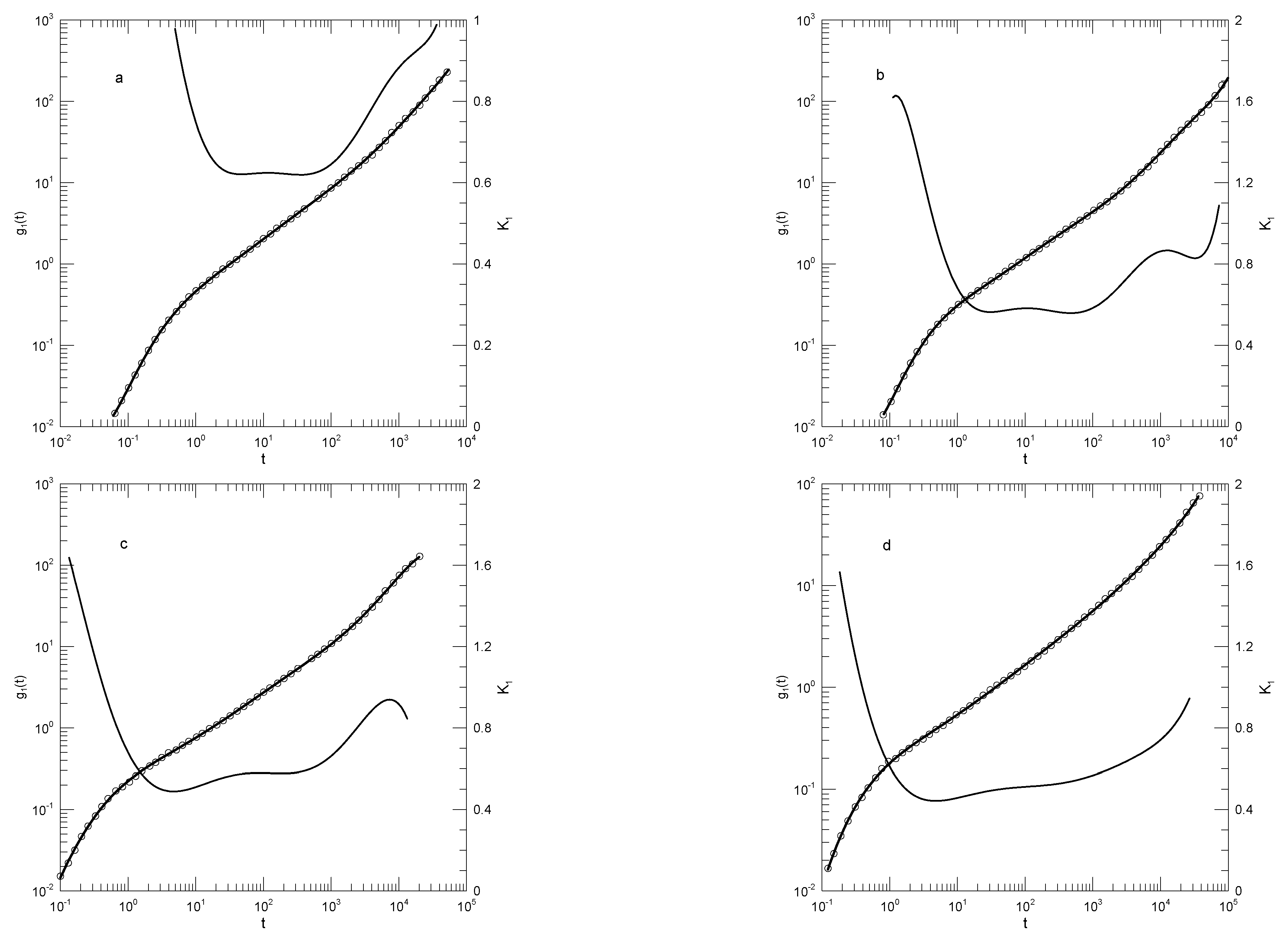
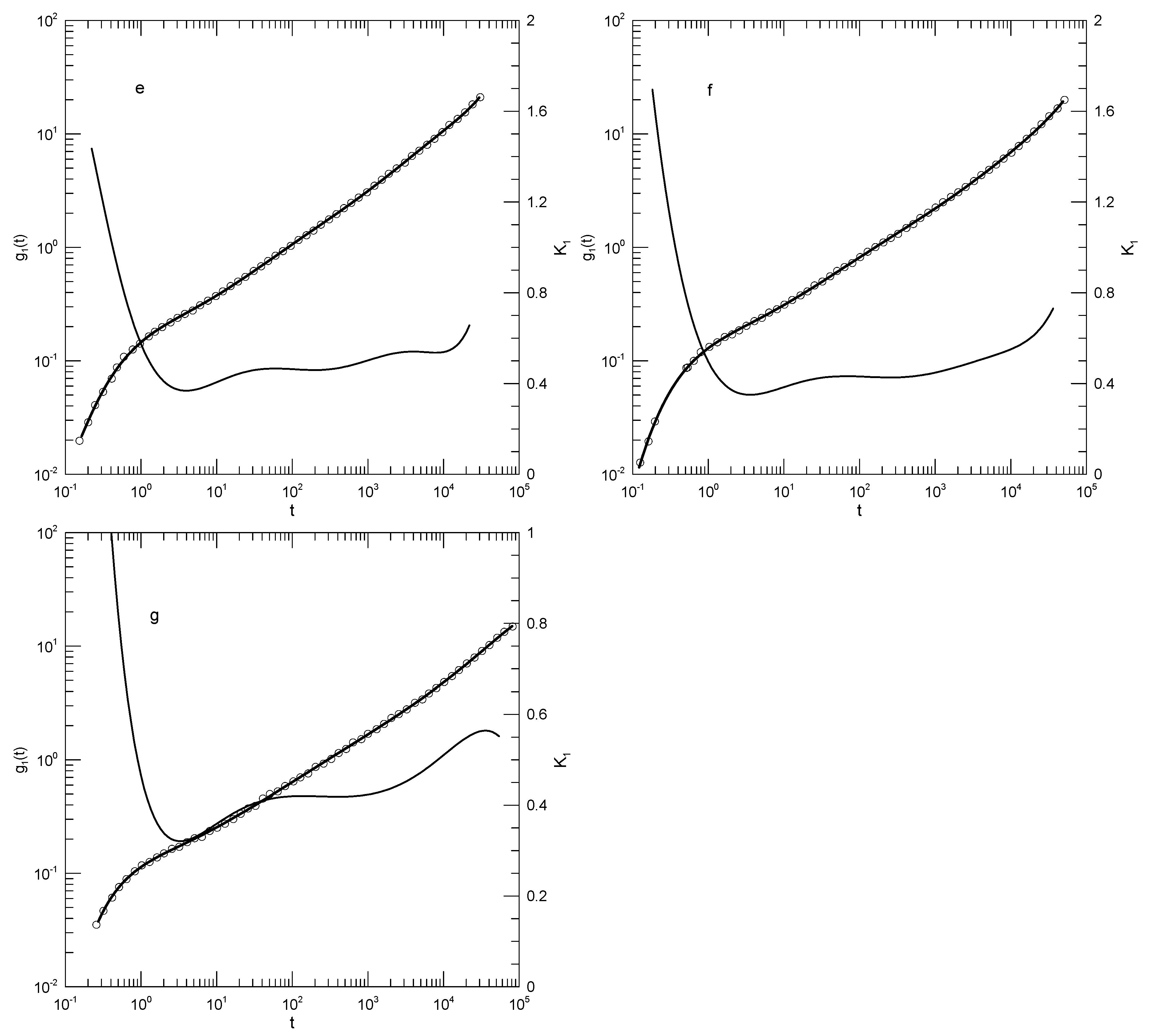
Figure 17.
A First part of Figure 17. Figure has been split to spread across two pages. (a) Mean-square displacement of the B beads of a melt of an A-B polymer blend with B mole fraction , based on Moreno, et al. [32] at temperatures (a) , (b) , (c) , and (d) . Heavy lines represent Moreno, et al.’s data, circles are eighth-order polynomial fits, and thin solid lines are first derivatives of the fits.
Figure 17.
B Second part of Figure 17. Figure has been split to spread across two pages. Mean-square displacement of the B beads in an A-B polymer blend melt with , based on Moreno, et al. [32] at temperatures (e) , (f) , and (g) . Heavy line show Moreno, et al.’s data, circles represent the eighth-order polynomial fits, and thin lines are the first derivatives of the polynomials.
Their first paper [33] considered simulations of an n-C120H242 melt. Their results for , , and appear in Figure 18. Figure 18, showing , is noteworthy for identifying a temporal region in which the mean-square displacement clearly does increase as a power law in time, namely, for , for . At larger t, first decreases to and then increases to . In contrast, only approaches power-law behavior, namely for center-of-mass motion drops rapidly to 0.75, then over close to two decades in time increases to 0.84 and finally increases to 1.0 or a bit larger. The behavior of is qualitatively similar to that of , namely after an initial rapid decrease in , there is an extended region in which is encountered.
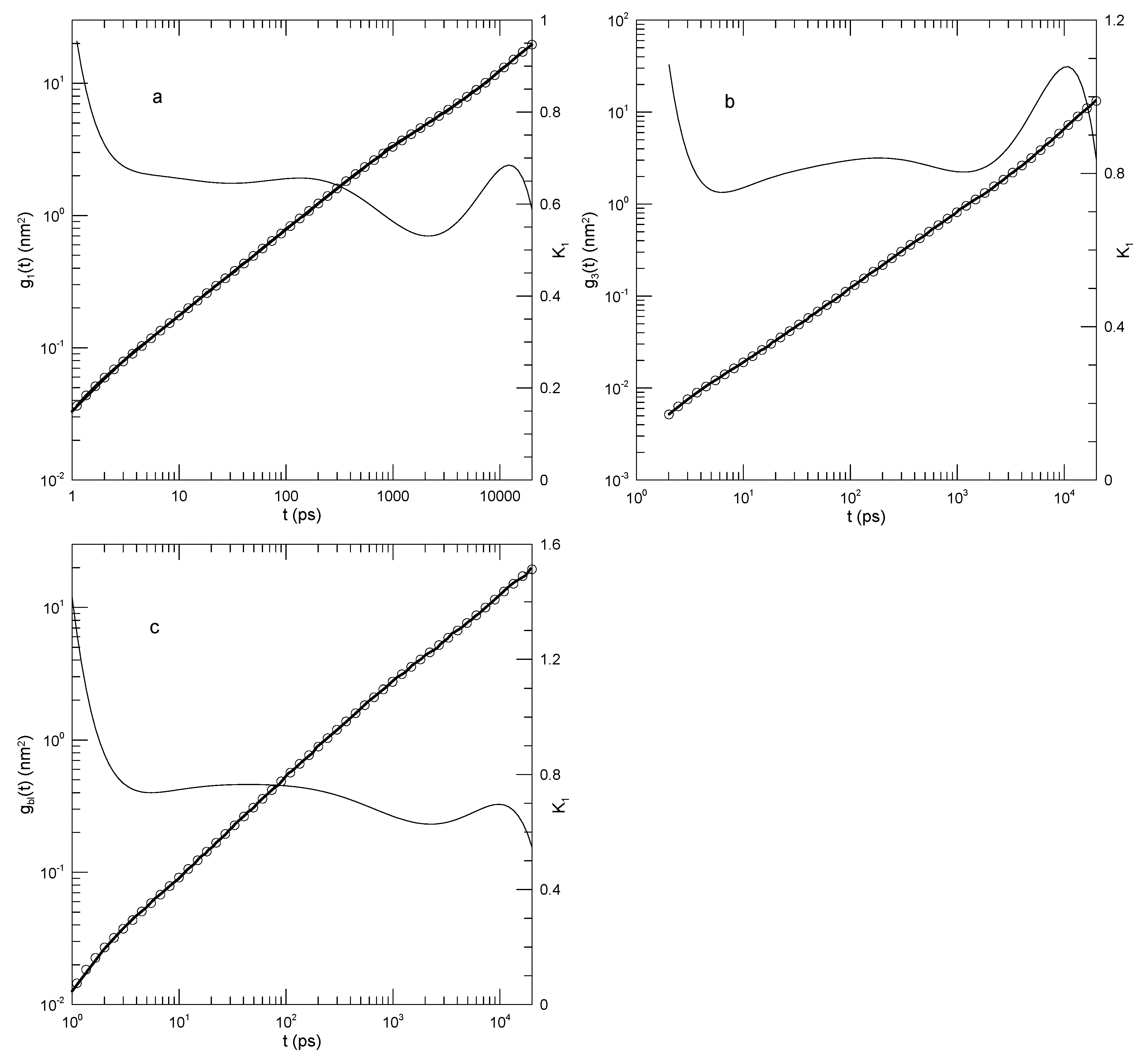
Figure 18.
Mean-square displacements of (a) individual atoms, (b) chain centers of mass, and (c) individual blobs for a simulated K melt of n-C120H242. Heavy lines indicate Padding and Briel’s data [33], circles represent eighth-order polynomial fits, and thin solid lines represent first derivatives of the polynomial fits.
In a further paper, Padding and Briels [35] report mean-square displacements of blobs – coarse-grained groups of 20 adjoining monomers – in simulated melts of linear polyethylene. Coarse-graining introduces complications. Most of the mechanical variables in the monomers of each blob must become bath variables, in the sense of the Mori-Zwanzig formalism, so that the blob equations of motion gain frictional and random-thermal forces. The blob-blob potential energy, determined as the blob-blob potential of average force from a united-atom simulation of the same system, is soft, so an alternative procedure was introduced to create the chain non-crossing constraint.
Figure 19 shows their results for for the 4-, 6-, and 50-blob chains. Their original figure (Figure 13 in their paper) also shows results for 10- and 20-bead polymer melts, but we encounter a limit of our procedure, namely if the data points are sufficiently overlapped, it becomes impossible to digitize the graph reporting the data. Having said that, curves for the three chain lengths are actually rather similar. The logarithmic derivative for each of the three curves begins at short times with a value close to 1.0, decreases to a minimum at times near , and then increases monotonically to a value close to 0.9. at the minimum is 0.60, 0.53, or 0.38, respectively, for the three chain lengths. Corresponding to the minimum in , has an inflection point. Except perhaps for the 4-blob chains at early times (), there are clearly no power-law regions at any time for any chain length. At times beyond the inflection point, of the two longer chains shows some additional structure, namely a region where it increases relatively slowly with increasing time.
In presenting their results, Padding and Briels [35] add to their log-log plot four straight lines to guide the eye, straight lines corresponding to power-law regimes, the labeled slopes being 1, 0.5, 0.4 (for the 50-blob chain) and 1. We find that the initial and terminal slopes are in reasonable agreement with Padding and Briels, namely approaches 1. Where Padding and Briels suggest a power-law region with a slope of 0.4, we identify an inflection point whose minimum slope is . The suggested line is in a region where there are few data points, and in which we find a slope that changes continuously, but their suggested line would be a tangent at some .
4. Discussion
This review considers simulations of polymer melts that determined polymer mean-square displacements . The time dependence of is of specific interest because widely-used theoretical models have as a core prediction that has power-law behavior . Equations 5–12 show the predicted in different time regimes. A particular focus of simulations has been a search for the exponent of 10.
We applied a new mathematical approach to test these predictions. As described in Section II, for each simulated system we determined the (time-dependent) logarithmic derivative of . At each t, from our approach gives an effective local value for . In any of the hypothetical power-law regimes, would a constant over an appreciable range of times. With very few exceptions, such a phenomenon—a constancy of —is not found. Instead, consistently shows a single more-or-less deep minimum, corresponding to a saddle point in the time dependence of .
We conclude that computer simulations serve to reject core predictions of the deGennes-Doi-Edwards description of a polymer melt. Efforts to extract power-law exponents from simulations of have been challenging. Our analysis indicates that the efforts failed because the hypothesized power-law behavior was not there to begin with.
An obvious objection to our conclusion is that, even with modern computational techniques, simulations can only examine relatively short polymers, polymers that are not heavily entangled. Indeed, the longest polymers examined here have as any as 2000 beads, perhaps corresponding to as many as forty entanglements. Of course, the deGennes-Doi-Edwards description does not actually indicate how many entanglements per chain are needed for the tube-reptation model to be applicable. There are also literature discussions as to what an entanglement is. A critic might therefore propose that the chains considered here were all unentangled. Nonetheless, as seen in equations 5–12, the deGennes-Doi-Edwards description also predicts the behavior of short chains, where there are few or no entanglements, and the behavior of long chains at short times, times too early for chain entanglements to affect polymer motion. These short-chain ( and perhaps short-time) predictions are indeed tested by our analysis. The predictions are incorrect; there is almost never power-law behavior; when there is, the exponent does not have the predicted value.
It should be entirely unsurprising that and of short polymers do not have the properties predicted in equations 5–8. These equations describe polymers that move in accordance with the Rouse model. However, as we have previously shown in an extensive review [12], for polymers in simulated melts the Rouse amplitudes and their time correlation functions have none of the properties associated with a Rouse-model polymer. In particular:
(i) Mean-square Rouse mode amplitudes do not scale as predicted by the Rouse model;
(ii) Rouse-mode time correlation functions do not decay with time as the exponentials predicted by the Rouse model;
(iii) Polymer bead displacements are not described by the independent Gaussian random processes that are assumed by the Rouse model; and
(iv) Rouse mode amplitudes are not always independent, i.e., it is not always true that for , as required by the Rouse model.
Proposals that polymer motions in the melt are described by the Rouse model, perhaps only at short times, are systematically inconsistent with extensive published simulations. This result should not be surprising, because the underlying Hamiltonian (properly, the underlying Rayleigh dissipation function) for short polymer chains in their melt is not the function assigned by Rouse. Rouse assumed that the forces on the beads of a polymer could be modelled as a series of independent Gaussian random processes, one for each bead. This assumption has been checked simulationally [12]. It is false. The displacement distribution function for the individual beads, the probability of finding a displacement during a time t, is in general not a Gaussian; instead, the non-Gaussianity parameter for the polymer bead displacements is found to be non-zero and time-dependent.
In almost all cases, we find that power-law behavior is absent. Theoretical models that predict that power-law behavior is important are rejected by our analysis. Now, it might be proposed that the predicted power-law regimes are separated by transition regimes in which power-law behavior is absent. It could be proposed that the transition regimes between power-law regimes are broad. Indeed, the latter proposal could be said to be supported by our analysis, namely, the transition regimes could have been more-or-less completely swallowed up the regions where power-law activity is found, reducing the power-law behavior to the slope at an inflection point. In that case, however, attempts to calculate any hypothesized power-law exponents are pursuing a theoretical fata morgana. A satisfactory theory of polymer melt dynamics would in this case need to focus on the broad transition regimes, not on the hypothesized regimes where power laws are encountered.
Funding
This research received no external funding.
Institutional Review Board Statement
Not applicable.
Informed Consent Statement
Not applicable.
Data Availability Statement
Data are contained within the article.
Acknowledgments
We thank Professors A. F. Behbahani and F. Schmid for supplying us with numerical tables of their mean-square displacement determinations.
Conflicts of Interest
The author declares no conflicts of interest.
References
- Phillies, G.D.J. Quantitative Interpretation of Simulated Polymer Mean-Square Displacements. Polymers 2025, 17, 516.
- Doi, M.; Edwards, S.F. The Theory of Polymer Dynamics. Clarendon Press: Oxford, U.K. 1988.
- de Gennes, P.-G. Scaling Concepts in Polymer Physics; Cornell U.P.: Ithaca, NY, USA, 1979.
- Rouse, P.E. A Theory of the Linear Viscoelastic Properties of Dilute Solutions of Coiling Polymers. J. Chem. Phys. 1953, 21, 1272–1280.
- Puetz, M.; Kremer, K.; Grest, G.S. What is the Entanglement Length in a Polymer Melt? Europhys. Lett. 2000, 49, 735–741.
- Schweizer, K.S. Mode-Coupling Theory of the Dynamics of Polymer Liquids: Qualitative Predictions for Flexible Chain and Ring Melts. J. Chem. Phys. 1989, 91, 5822–5839.
- Schweizer, K.S. Microscopic Theory of the Dynamics of Polymeric Liquids: General Formulation of a Mode-Mode-Coupling Approach. J. Chem. Phys. 1989, 91, 5802–5821.
- Doob, J.L. The Brownian Movement and Stochastic Equations. Ann. Math. 1942, 43, 351–369.
- Phillies, G.D.J. The Gaussian Diffusion Approximation is Generally Invalid in Complex Fluids. Soft Matter 2015, 11, 580–586.
- Phillies, G.D.J. Phenomenology of Polymer Solution Dynamics. Cambridge University Press: Cambridge, U.K., 2011.
- Phillies, G.D.J. Kirkwood-Riseman Model in Non-Dilute Polymeric Fluids. Polymers 2023, 15, 3216 (2023).
- Phillies, G.D.J. Simulational Tests of the Rouse Model. Polymers 2023, 15, 2615 (2023).
- Silk Scientific, Provo, Utah.
- Behbahani, A.F.; Schmid, F. Relaxation Dynamics of Entangled Linear Polymer Melts via Molecular Dynamics Simulations. Macromolecules 2025, 58, 767–786.
- Grest, G.S.; Kremer, K. Molecular Dynamics Simulation for Polymers in the Presence of a Heat Bath. Phys. Rev. A 1986, 33, 3628–3631.
- Weeks, J.D.; Chandler, D.; Andersen, H.C. Role of Repulsive Forces in Determining the Equilibrium Structure of Simple Liquids. J. Chem. Phys. 1971, 54, 5237–5247.
- Benneman, C.; Paul, W.; Binder, K.; B. Duenweg; B. Molecular-Dynamics Simulations of the Thermal Glass Transition in Polymer Melts: α-Relaxation Behavior. Phys. Rev. E 1998, 57, 843–851.
- Chang, R.; Yethiraj, A. Can Polymer Chains Cross Each Other and Still Be Entangled? Macromolecules 2019, 52, 2000–2006.
- Tsalikis, D.G.; Koukoulas, T.; Mavrantzas, V.G.; Pasquino, R.; Vlassopoulos, D.; Pyckhout-Hintzen, W.; Waschnewski, A.; Monkenbusch, M.; Richter, D. Microscopic Structure, Conformation, and Dynamics of Ring and Linear Poly(ethylene oxide) Melts from Detailed Atomistic Molecular Dynamics Simulation: Dependence on Chain Lengths and Direct Comparison with Experimental Data. Macromolecules 2017, 50, 2565–2584.
- Fischer, J.; Pascheck, D.; Geiger, A.; Sadowski, G. Modeling of Aqueous Poly(oxyethylene) Solutions: 1. Atomistic Simulations. J. Phys. Chem. B 2008, 112, 2388–2398.
- Fischer, J.; Pascheck, D.; Geiger, A.; Sadowski, G. Addition and Corrections in Modeling of Aqueous Poly(oxyethylene) Solutions: Atomistic Simulations. J. Phys. Chem. B 2008, 112, 8849–8850.
- Takahashi, K.Z.; Nishimura, R.; Yasuoka, K.; Masabuchi, Y. Molecular Dynamics Simulations for Resolving Scaling Laws of Polyethylene Melts. Polymers 2017, 9, 24.
- Peng, W.; Ranganathan, R.; Keblinski, P.; Ozisik, R. Viscoelastic and Dynamic Properties of Well-Mixed and Phase-Separated Binary Polymer Blends: A Molecular Dynamics Simulation Study. Macromolecules 2017, 50, 6293–6302.
- Hsu, H.-P.; Kremer, K. Static and Dynamic Properties of Large Polymer Melts in Equilibrium. J. Chem. Phys. 2016, 144, 154907.
- Brodeck, M.; Alvarez, F.; Moreno, A.J.; Colmenero, J.; Richter, D. Chain Motion in Nonentangled Dynamically Asymmetric Polymer Blends: Comparison between Atomistic Simulations of PEO/PMMA and a Generic Bead-Spring Model. Macromolecules 2010, 43, 3036–3051.
- Stephanou, P.S.; Baig, C.; Tsolou, G.; Mavrantzas, V.G.; Kroeger, M. Quantifying Chain Reptation in Entangled Polymer Melts: Topological and Dynamical Mapping of Atomistic Simulation Results onto the Tube Model. J. Chem. Phys. 2010, 132, 124904.
- Everaers, R.; Sukumaran, S.K.; Grest, G.S.; Svaneborg, C.; Sivasubramanian, A.; Kremer, K. Rheology and Microscopic Topology of Entangled Polymeric Liquids. Science 2004, 303, 823–826.
- Karayiannis, N. Ch.; Mavrantzas, V.G. Hierarchical Modelling of the Dynamics of Polymers with a Nonlinear Molecular Architecture: Calculation of Branch Point Friction and Chain Reptation Time of H-Shaped Polyethylene Melts from Long Molecular Dynamics Simulations. Macromolecules 2005, 38, 8583–8596.
- Tsolou, G.; Mavrantzas, V.G.; Theodorou, D.N. Detailed Atomistic Molecular Dynamics Simulation of cis-1-4-Poly(butadiene). Macromolecules 2005, 38, 1478–1492.
- Likhtman, A.E.; Sukumaran, S.K.; Ramirez, J. Linear Viscoelasticity from Molecular Dynamics Simulation of Entangled Polymers. Macromolecules 2007, 40, 6748–6757/.
- Zhou, Q.; Larson, R.G. Direct Calculation of the Tube Potential Confining Entangled Polymers. Macromolecules 2006, 39, 6737–6743.
- Moreno, A.J.; Colmenero, J. Is There a Higher-Order Mode-Coupling Transition in Polymer Blends. J. Chem. Phys. 2006, 124, 184906.
- Padding, J.T.; Briels, W.J. Zero Shear Stress Relaxation and Long Time Dynamics of a Linear Polethylene Melt: A Test of Rouse Theory. J. Chem. Phys. 2001, 114, 8685–8693.
- Padding, J.T.; Briels, W.J. Uncrossability Constraints in Mesoscopic Polymer Melt Simulations: Non-Rouse Behavior of C120H242. J. Chem. Phys. 2001, 115, 2846–2859.
- Padding, J.T.; Briels, W.J. Time and Length Scales of Polymer Melts Studied by Coarse-Grained Molecular Dynamics Simulations. J. Chem. Phys. 2002, 117, 925–943.
- Padding, J.T.; Briels, W.J. Coarse-Grained Molecular Dynamics Simulations of Polymer Melts in Transient and Steady Shear Flow. J. Chem. Phys. 2003, 118, 10276–10286.
Figure 1.
Mean-square bead displacements (thick lines) of melts of short Kremer-Grest bead-spring chains, based on simulations of Behbahani and Schmid [14], together with fits to eighth-order polynomials (circles) and the corresponding first logarithmic derivatives (thin lines). Chains contained (a) 10, (b) 30, (c) 50, or (d) 100 beads.
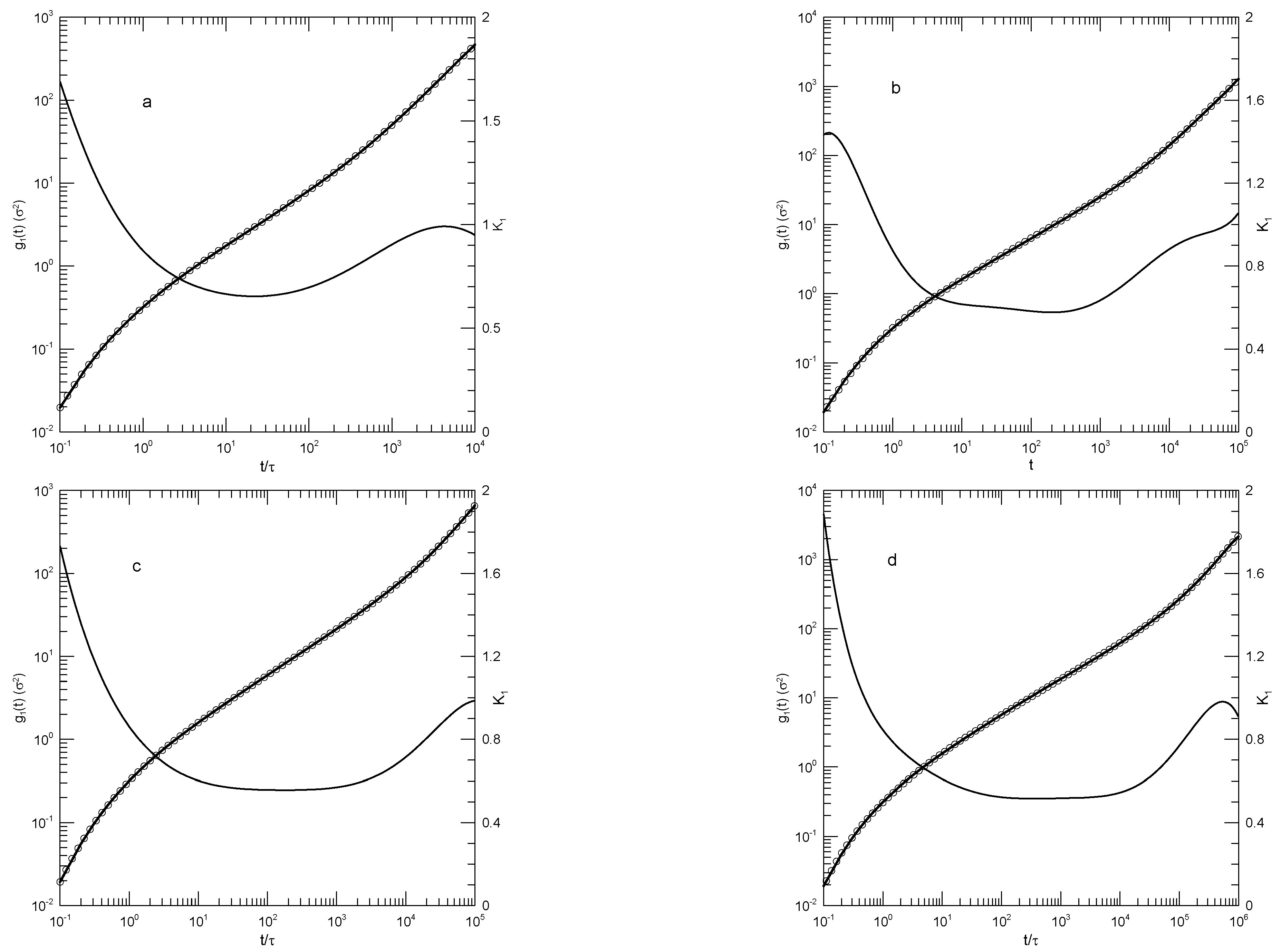
Figure 2.
Mean-square bead displacements (thick lines under circles) of melts of long Kremer-Grest bead-spring chains, based on simulations of Behbahani and Schmid [14], together with polynomial fits (circles) and the corresponding first logarithmic derivatives (thin lines). Chains contained (a) 150, (b) 200, (c) 400, or (d) 1000 beads. Polynomial fits were to eighth-order polynomials via linear-least-squares, except for the 400-bead polymers, for which a tenth-order polynomial was used.
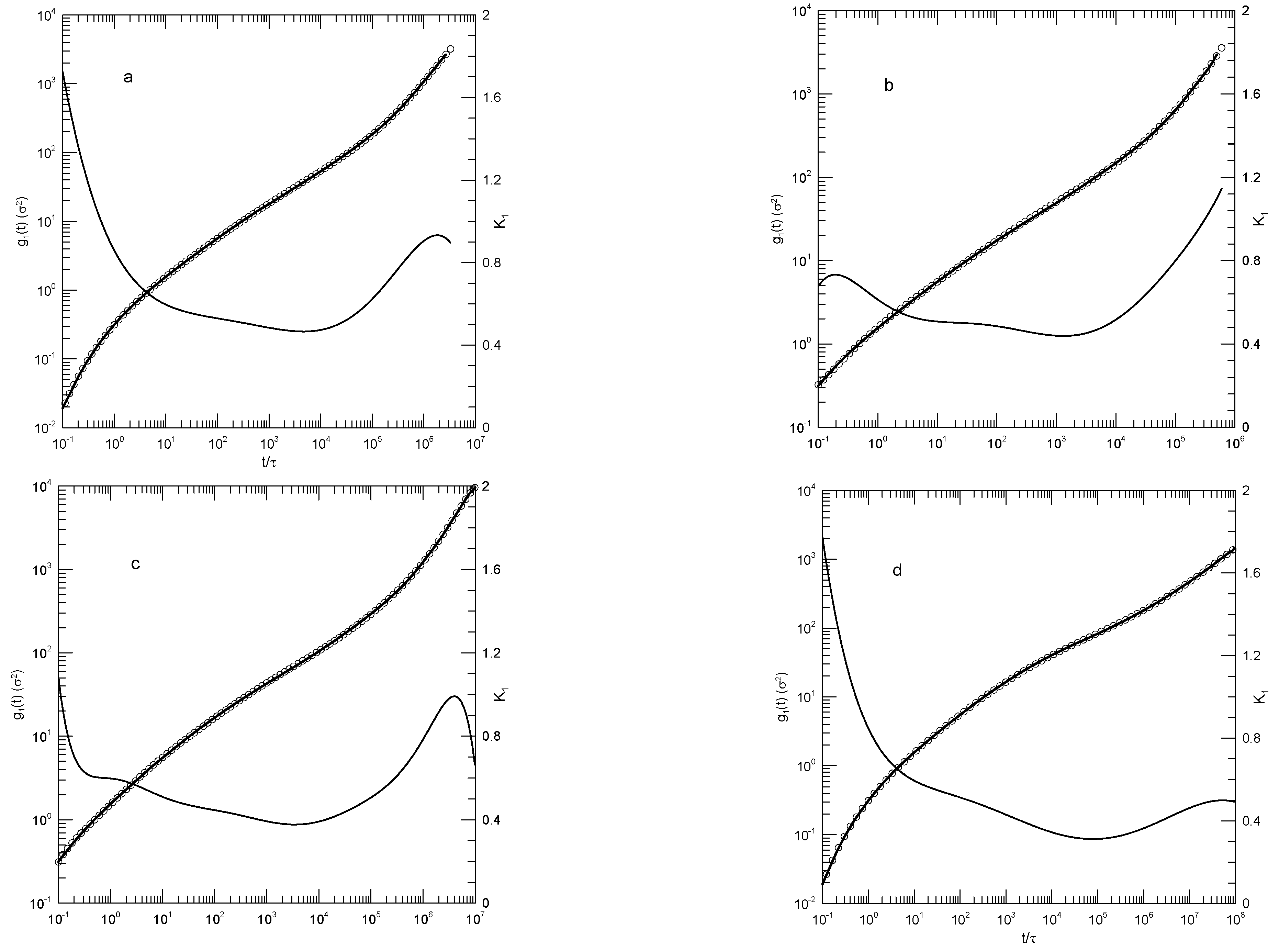
Figure 3.
Mean-square bead displacements of central beads (thick lines under circles) of melts of 1000-bead Kremer-Grest bead-spring chains, based on simulations of Behbahani and Schmid [14], together with a fit to an eighth-order polynomial (circles) and its first logarithmic derivatives (thin lines).
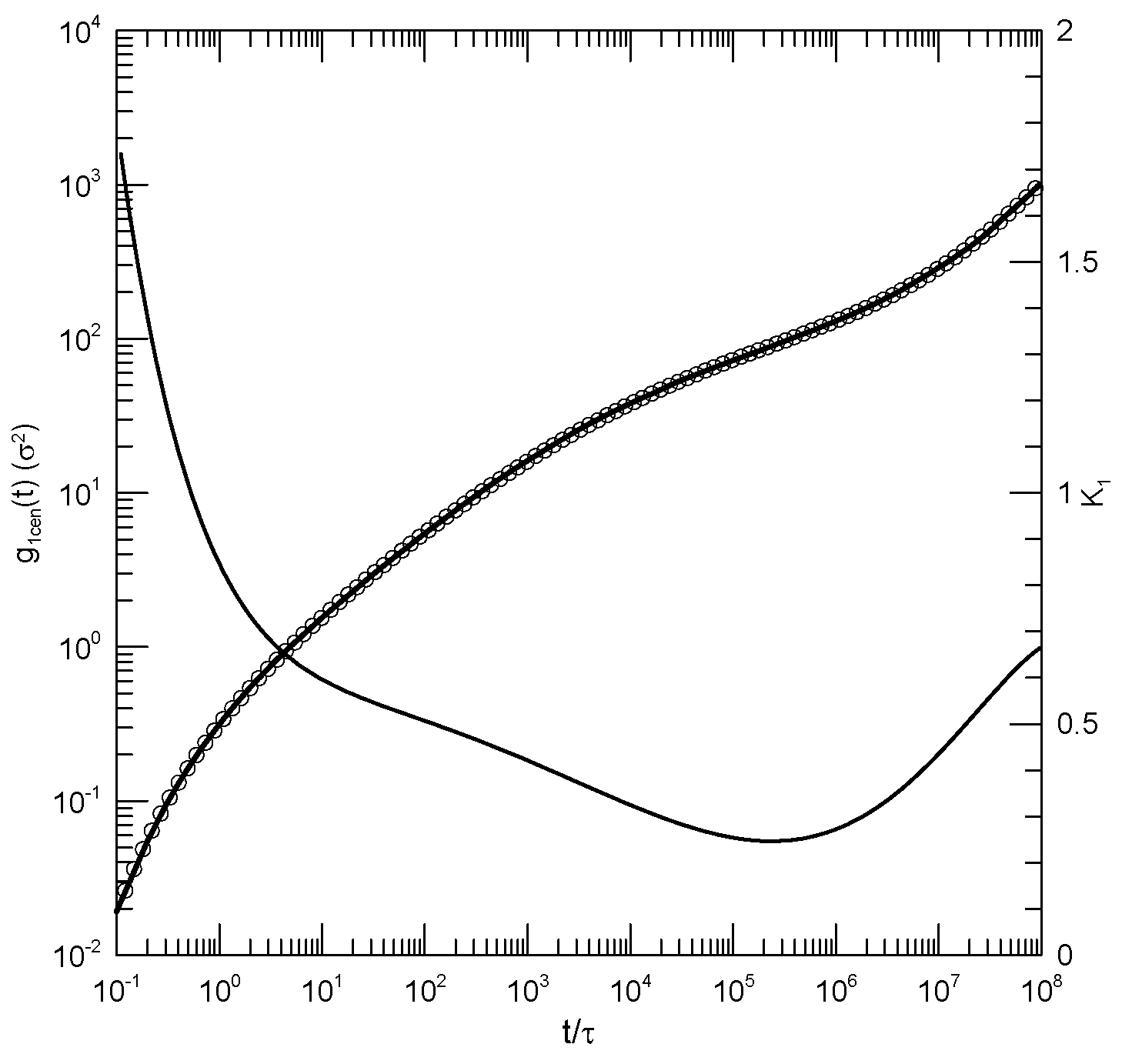
Figure 4.
Mean-square center-of-mass displacements (thick lines under circles) of melts of short Kremer-Grest bead-spring chains, based on simulations of Behbahani and Schmid [14], together with polynomial fits (circles) and their first logarithmic derivatives (thin lines). Chains contained (a) 10, (b) 30, (c) 50, or (d) 100 beads. Polynomial fits were to eighth-order polynomials via linear-least-squares.
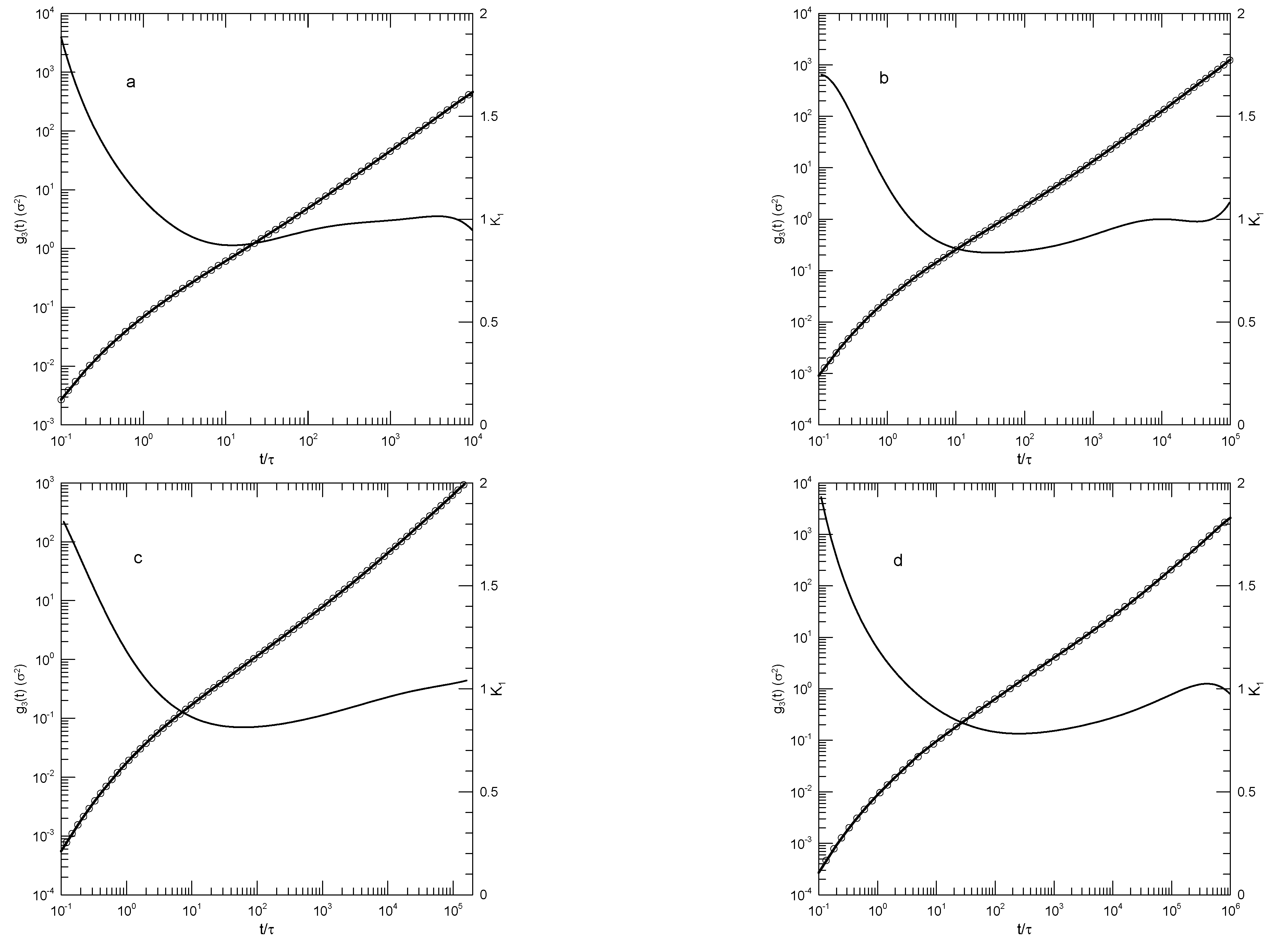
Figure 5.
Mean-square center-of-mass displacements (thick lines under circles) of melts of long Kremer-Grest bead-spring chains, based on simulations of Behbahani and Schmid [14], together with polynomial fits (circles) and their first logarithmic derivatives (thin lines). Chains contained (a) 150, (b) 200, (c) 400, or (d) 1000 beads. Polynomial fits were to eighth-order polynomials via linear-least-squares.

Figure 6.
Mean-square center-of-mass (Figures a-c) and central-bead (Figures d-f) mean-square displacement measurements (heavy lines) of a melt of 256-bead chains, based on the simulations of Chang and Yethiraj [18], together with polynomial fits (circles) and first logarithmic derivatives (thin lines). Here takes values (a,d) 0.4 or 0.45, (b,e) 0.5, and (c,f) 0.6. Polynomial fits were to eighth-order polynomials via linear-least-squares.
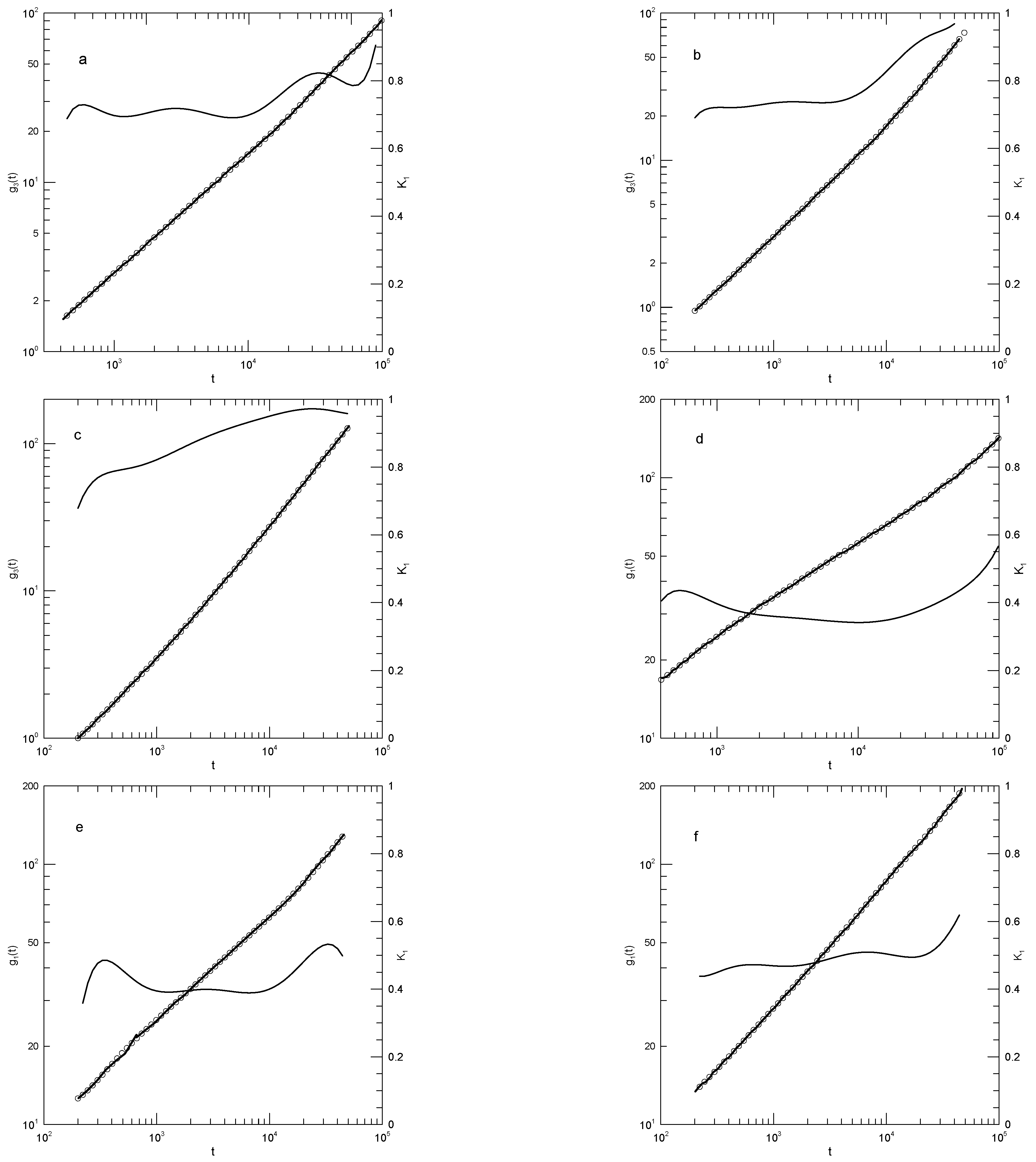
Figure 7.
Mean-square bead displacements (heavy lines) of linear (Figures a, c, e) and ring (Figures b, d, f) polyethylene oxides, as determined by the united-atom simulations of Tsalikis, et al. [19], together with polynomial fits (circles) and their first logarithmic derivatives (thin lines). Polymer lengths were 120 beads (Figures a, b), 227 beads (Figures c, d), and 455 beads (Figures e, f). Polynomial fits were to eighth-order polynomials via linear-least-squares.
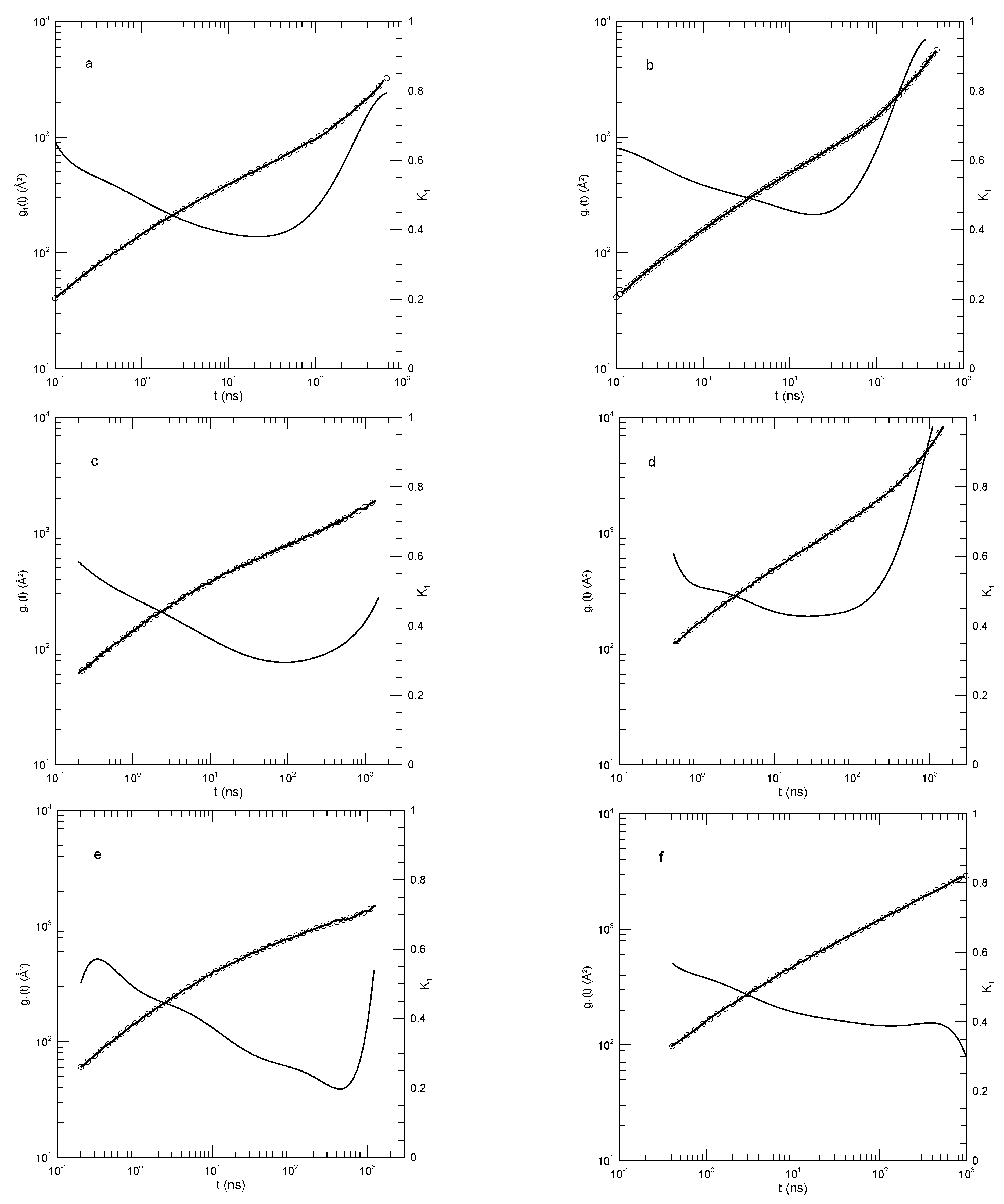
Figure 8.
Mean-square bead displacements (thick lines) of linear polyethylenes, nominal molecular weights (1) 422, (b) 703, (c) 983, (d) 1405, (e) 2106, and (f) 2807 Da, from Takahashi, et al. [22], together with eighth-order polynomial fits (circles) and their first logarithmic derivatives (thin lines).
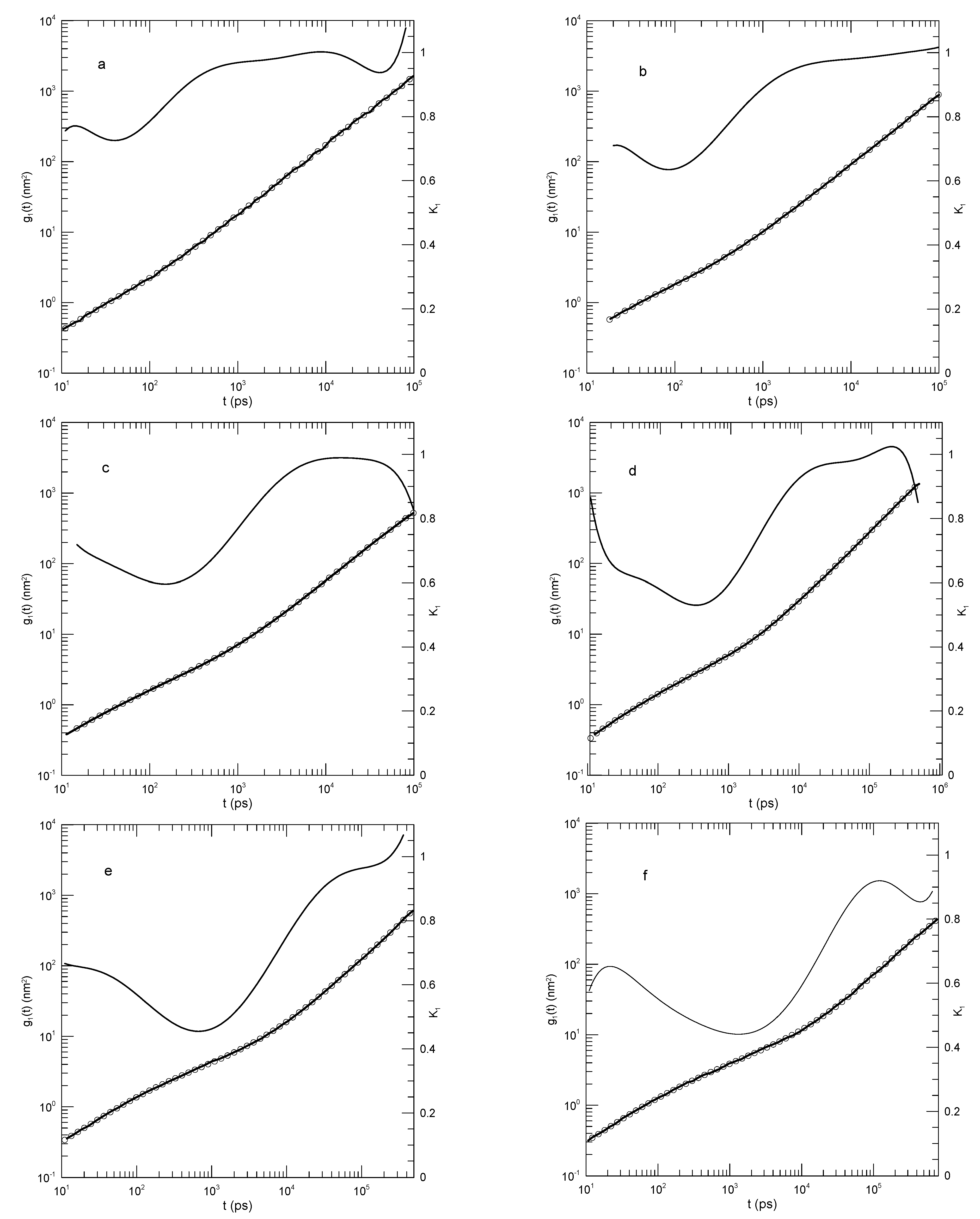
Figure 9.
Mean-square bead displacements (thick lines) of B beads in (a,b) non-phase-separated mixtures, (c) the pure-B melt, and (d) in a phase-separated mixture, from Peng, et al. [23], together with polynomial fits (circles) and first logarithmic derivatives (thin lines). The A chains had lengths of (a) 5, (b) 20, and (d) 50 beads.
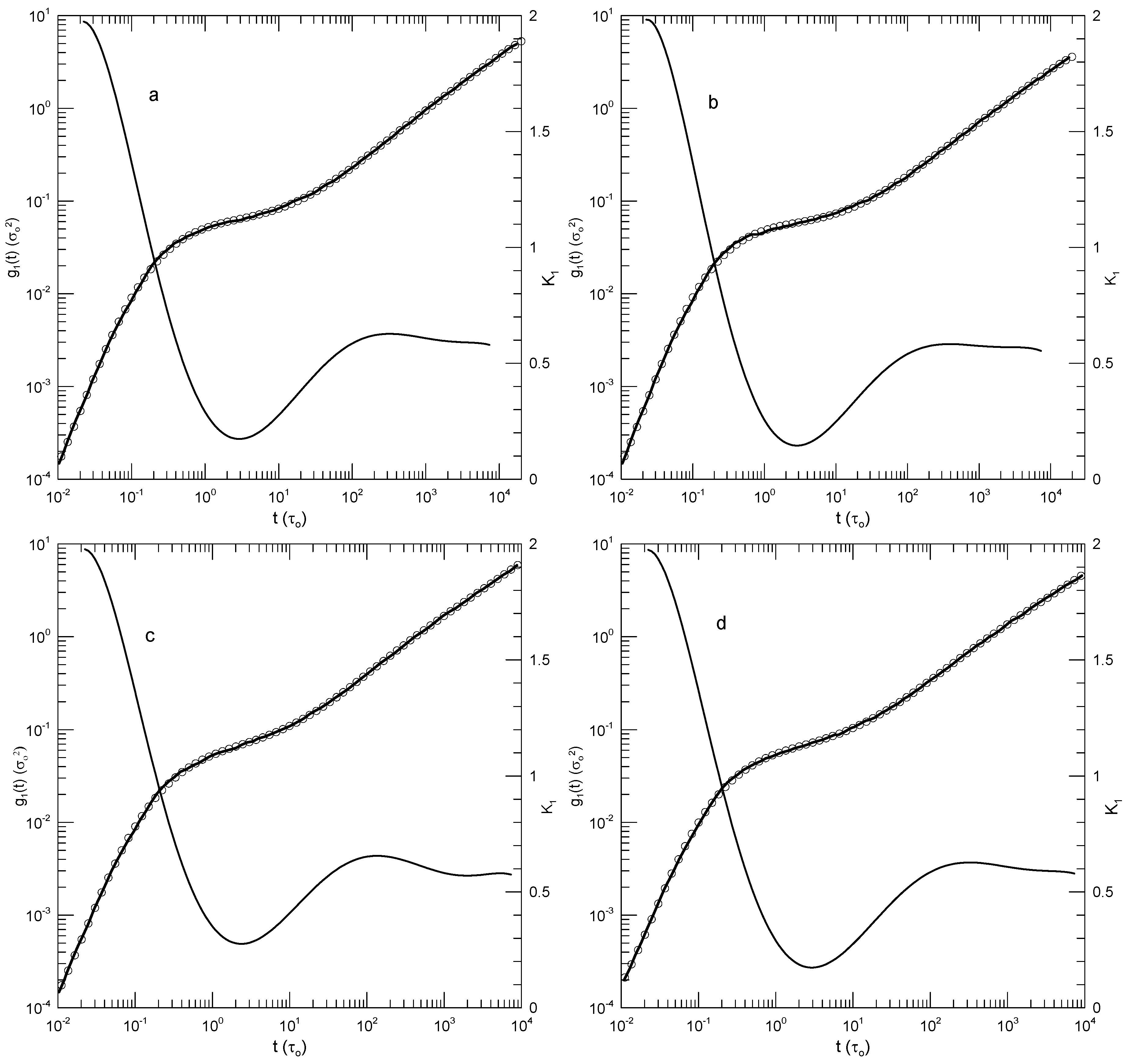
Figure 10.
Hsu and Kremer’s results for (a-c) 500-bead and (d-f) 2000-bead chains [24]. Graphs show mean-square motions of (a,d) individual beads, (b,e) bead motions relative to chain centers of mass, and (c,f) chain centers of mass. Heavy lines are the simulations, circles are polynomial fits, and thin solid lines represent first derivatives .
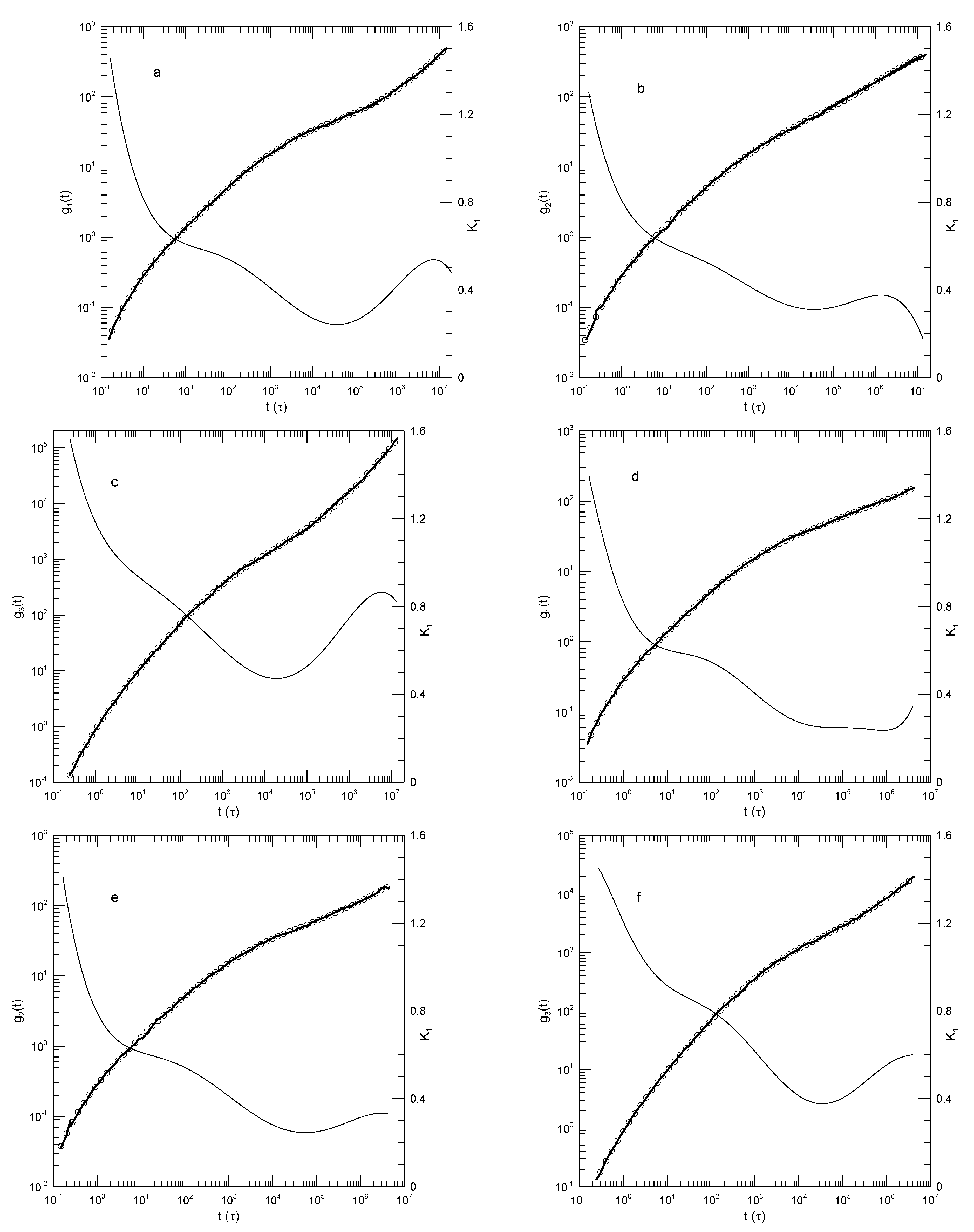
Figure 11.
Mean-square displacements of individual PEO hydrogen atoms in PEO-PMMA blend melts at temperatures (a) 500, (b) 400, (c) 350, and (d) 300 K, from Brodeck, et al. [25]. Heavy lines indicate Brodeck, et al.,’s results, circles are the eighth-order polynomial fits, and thin solid lines represent first logarithmic derivatives .
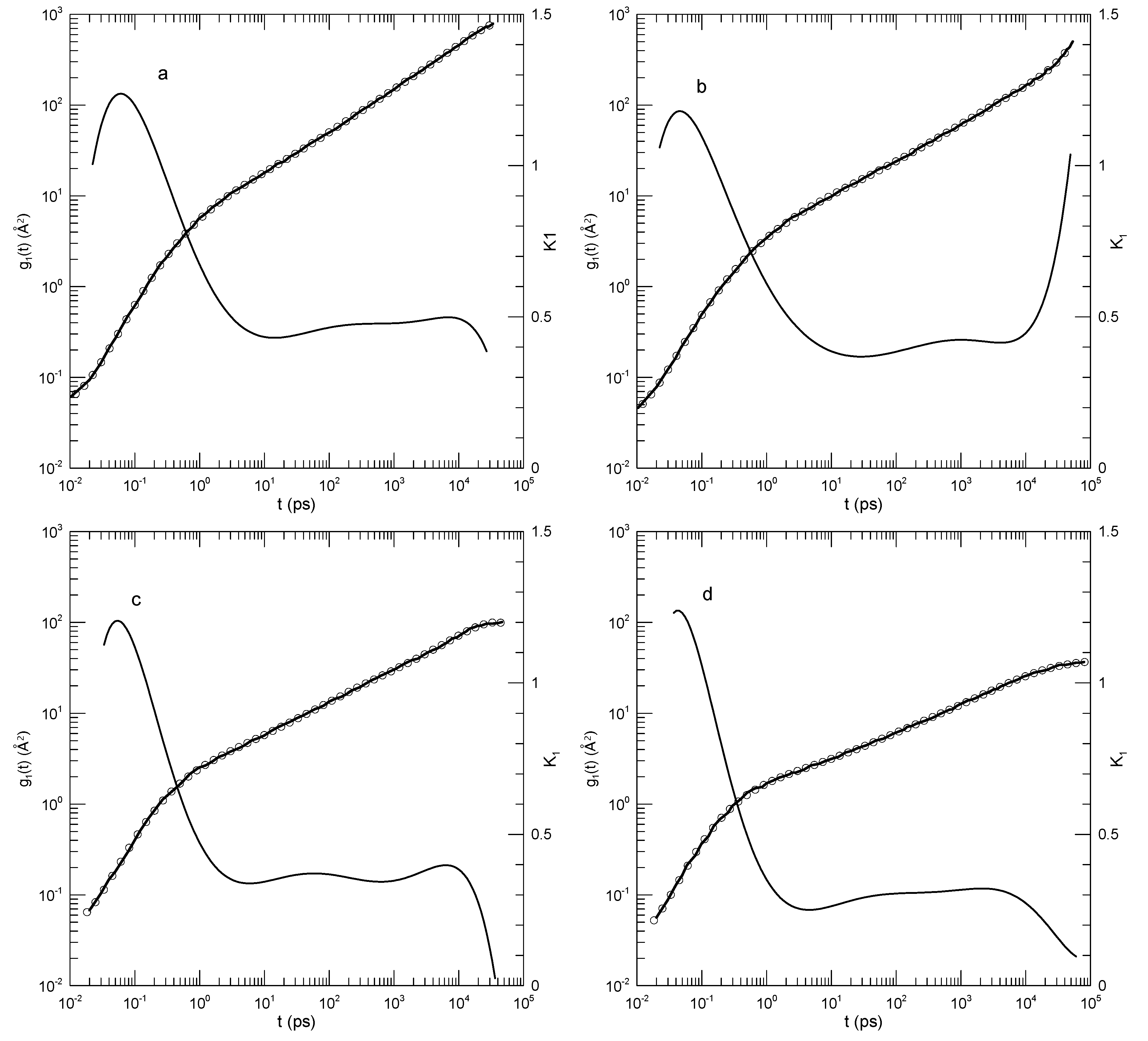
Figure 12.
Mean-square displacements of chain centers-of-mass of PEO molecules in PEO-PMMA blend melts at temperatures (a) 500, (b) 400, (c) 350, and (d) 300 K from Brodeck, et al. [25]. Heavy lines indicate Brodeck, et al.,’s results, circles are the eighth-order polynomial fits, and thin solid lines represent first logarithmic derivatives .
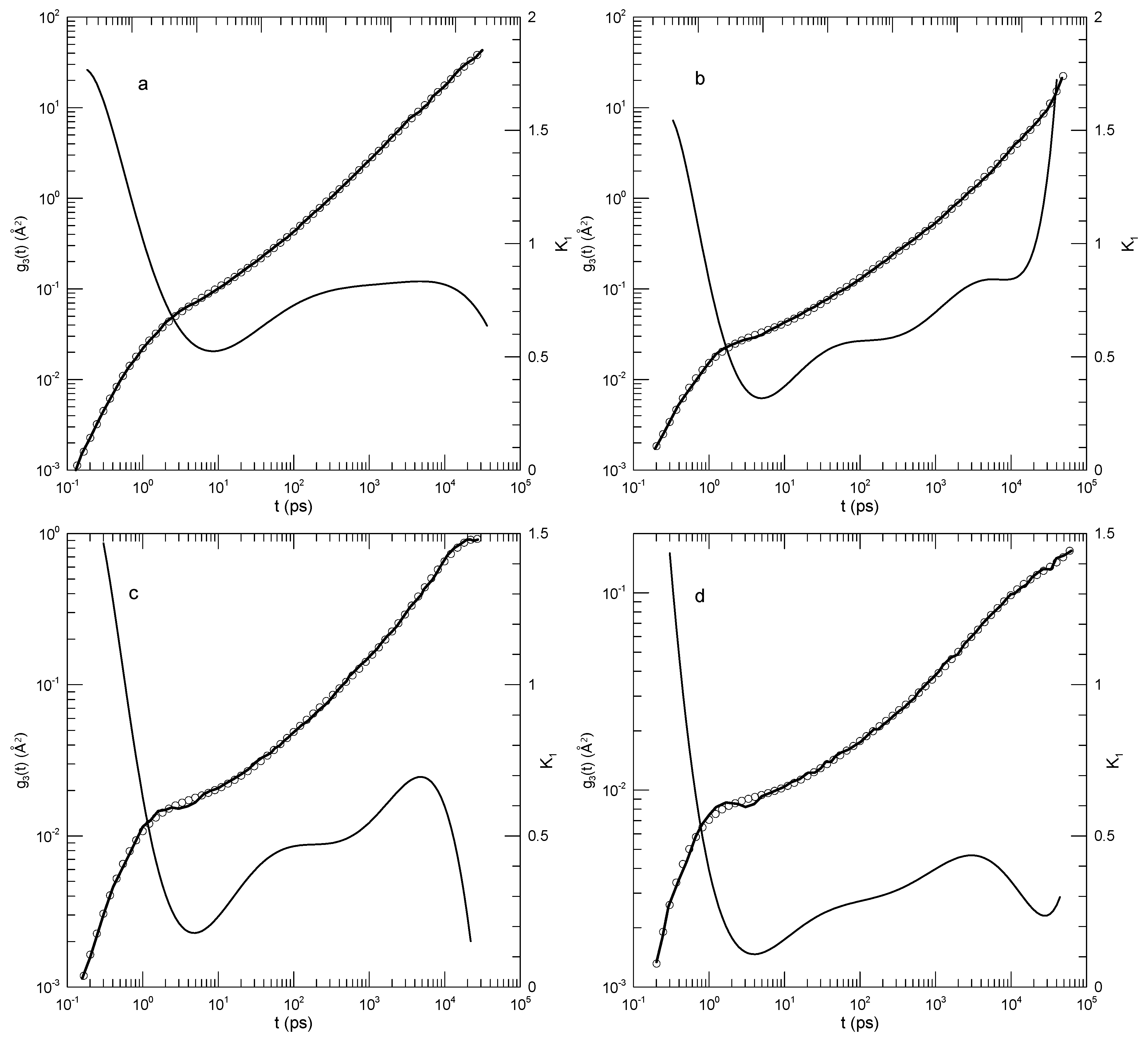
Figure 14.
Mean-square displacements of central beads of (a) 50-, (b) 100-, (c) 200-, and (d) 350-bead simulated Grest-Kremer polymer melts, based on Likhtman, et al. [30]. Here heavy lines are digitizations of Likhtman, et al.,’s data, circles represent eighth-order polynomial fits, and thin solid lines show the first derivatives of the two polynomial fits.
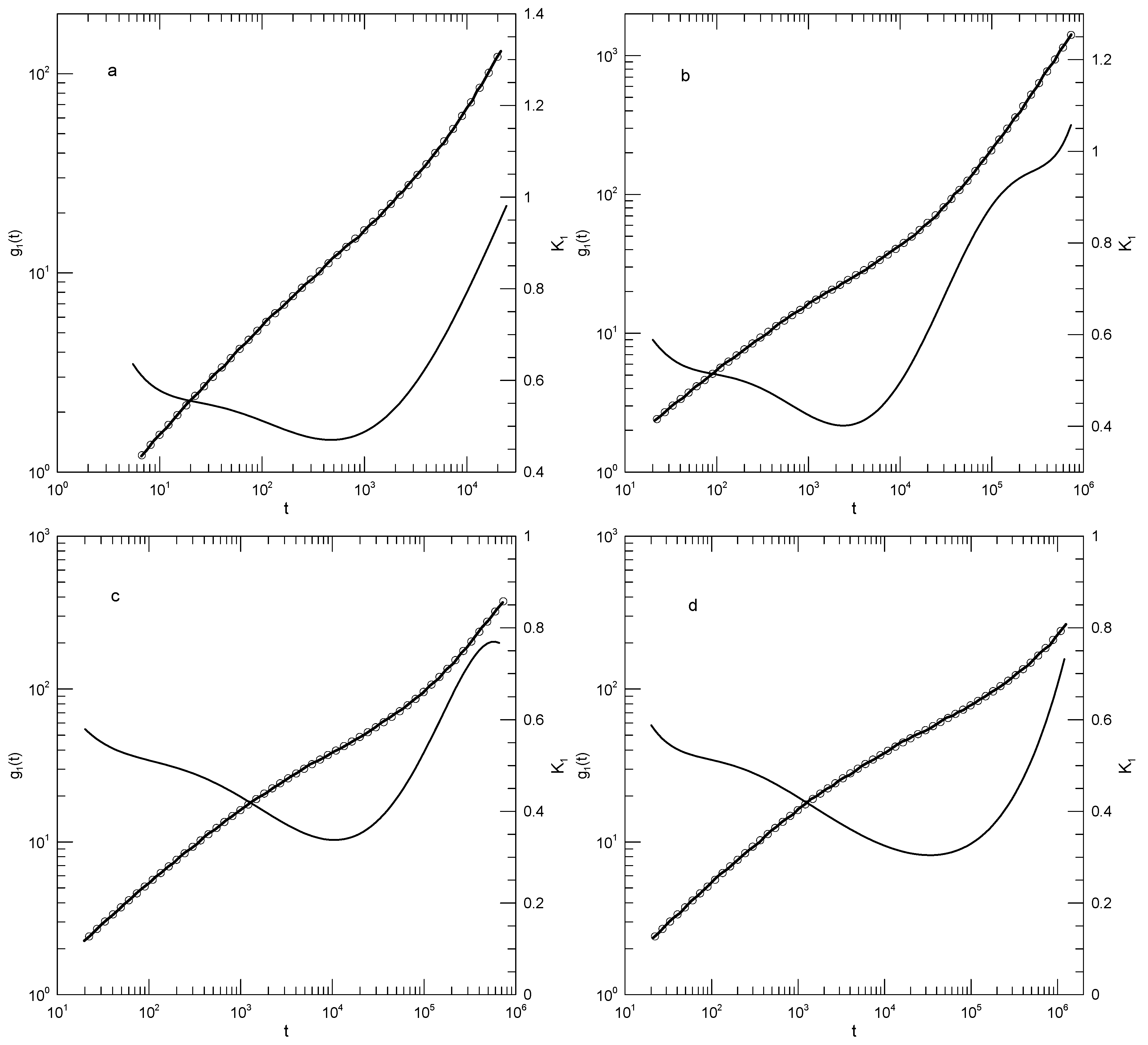
Figure 15.
Mean-square displacement of a polymer’s beads relative to its center of mass, for bead-spring polymers having lengths (a) 150 and (b) 300 beads, based on Zhou and Larson [31]. Heavy lines are digitizations of Zhou and Larson’s data, circles represent eighth-order polynomial fits, and thin solid lines show the first derivative of each polynomial fit.
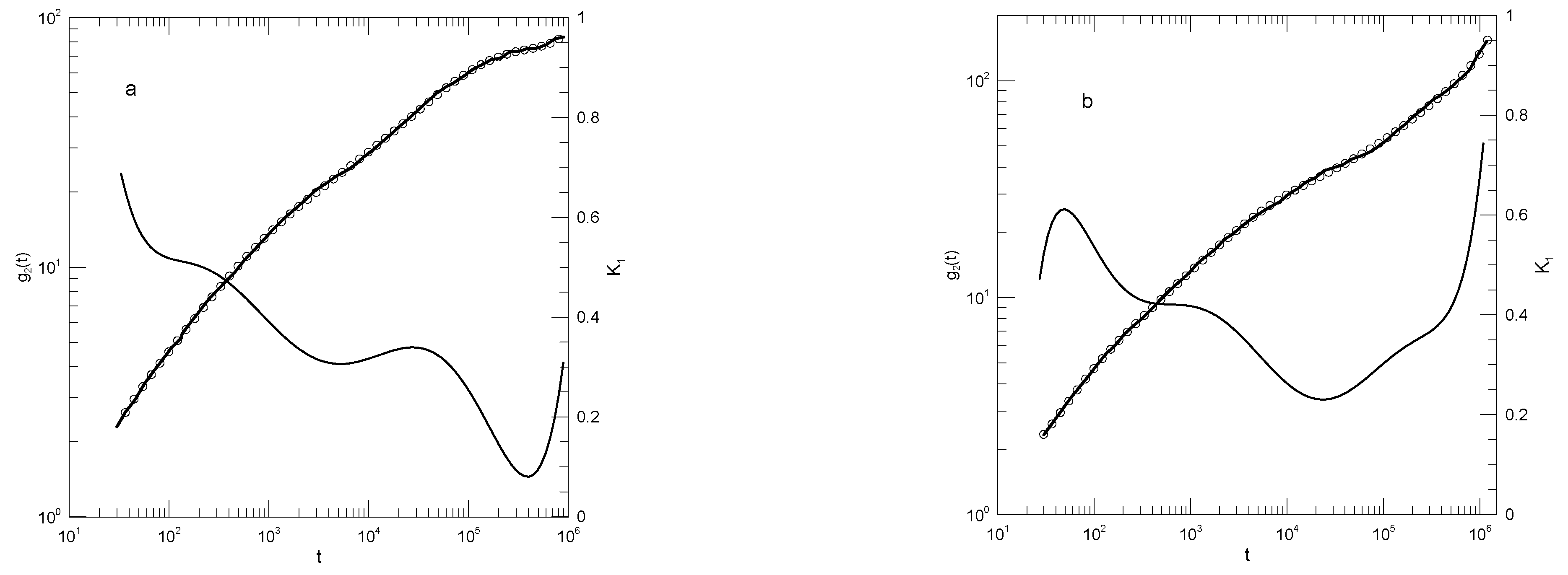
Figure 16.
(a)Mean-square displacement of individual beads of a pure B melt, data from Moreno, et al. [32] at temperatures (a) , (b) , (c) , (d) , (e) , and (f) . Heavy lines are digitizations of Moreno, et al.’s data, circles represent eighth-order polynomial fits, and thin solid lines are first derivatives of the polynomial fits.
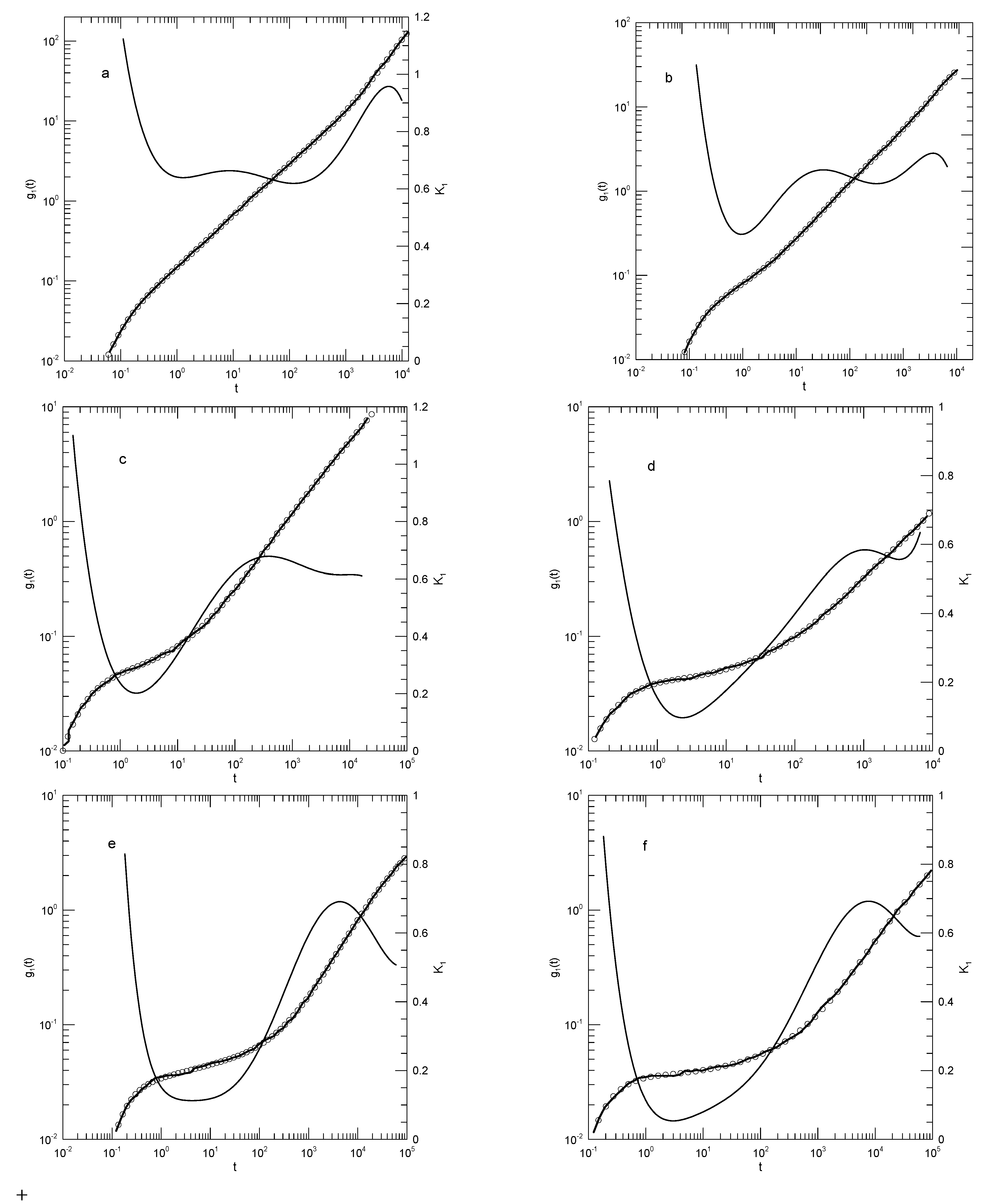
Figure 19.
Mean-square displacements of blobs in polyethylene melts containing (a) 4, (b) 6, or (c) 50 blobs (and, correspondingly, (a) 80, (b) 120, or (c) 1000 monomers). Heavy lines indicate Padding and Briel’s data, circles show the eighth-order polynomial fits, and thin solid lines represent , the first derivative of the polynomial fits.
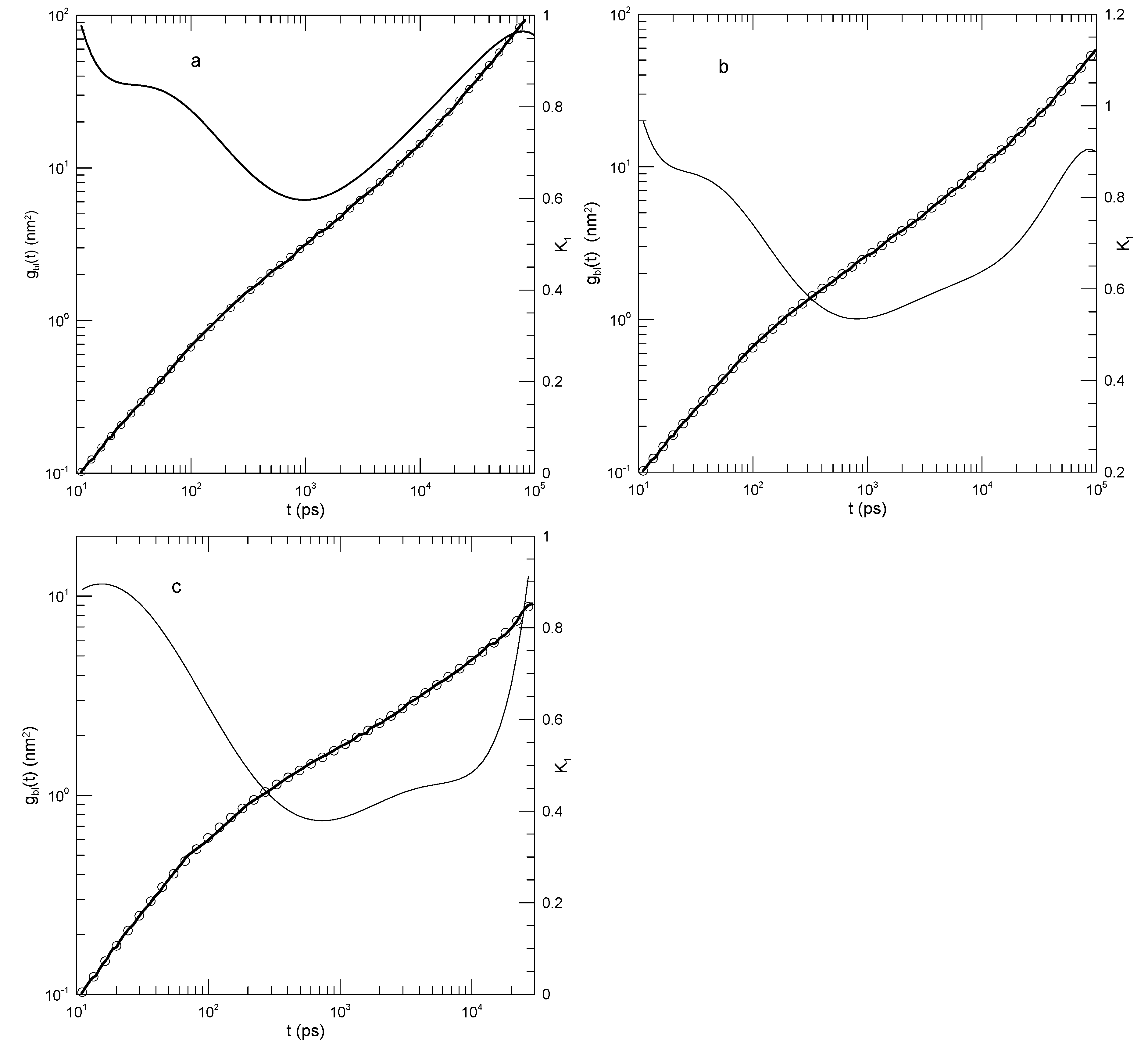

Table 1.
Value of the logarithmic derivative at the inflection point, for different polymer lengths N, as determined from or as measured by Behbahani and Schmid. [14]
Table 1.
Value of the logarithmic derivative at the inflection point, for different polymer lengths N, as determined from or as measured by Behbahani and Schmid. [14]
| N | ||
| 10 | 0.65 | 0.87 |
| 30 | 0.59 | 0.84 |
| 50 | 0.56 | 0.82 |
| 100 | 0.52 | 0.78 |
| 150 | 0.47 | 0.74 |
| 200 | 0.44 | 0.69 |
| 400 | 0.38 | 0.62 |
| 1000 | 0.31 | 0.50 |
Table 2.
Slopes at inflection points in the results of Hsu and Kremer [24]. *power law regime.
Table 2.
Slopes at inflection points in the results of Hsu and Kremer [24]. *power law regime.
| function | Figure | N | Slope |
| 10a | 500 | 0.24 | |
| 10b | 500 | 0.31 | |
| 10c | 500 | 0.47 | |
| 10d | 2000 | * | |
| 10e | 2000 | 0.25 | |
| 10f | 2000 | 0.38 |
Disclaimer/Publisher’s Note: The statements, opinions and data contained in all publications are solely those of the individual author(s) and contributor(s) and not of MDPI and/or the editor(s). MDPI and/or the editor(s) disclaim responsibility for any injury to people or property resulting from any ideas, methods, instructions or products referred to in the content. |
© 2025 by the authors. Licensee MDPI, Basel, Switzerland. This article is an open access article distributed under the terms and conditions of the Creative Commons Attribution (CC BY) license (http://creativecommons.org/licenses/by/4.0/).
Copyright: This open access article is published under a Creative Commons CC BY 4.0 license, which permit the free download, distribution, and reuse, provided that the author and preprint are cited in any reuse.


