Submitted:
21 March 2025
Posted:
21 March 2025
You are already at the latest version
Abstract
In this study, effect of inlet turbulence intensity on the friction coefficient for transitional boundary layer has been investigated computationally. For this purpose, two equation turbulence models of Std. k-ε, RNG k-ε, Std. k-ω ve SST k-ω have been compared with Gamma-Theta (GT) transitional model, and it has been found that Gamma Theta model is the most consistent model with the experimental values of the ERCOFTAC T3A test case. Then, the effect of inlet turbulence intensity on the friction coefficient has been computed by using this Gamma-Theta model. Transition from laminar to turbulence is shortened with increasing turbulence intensity by changing it from 0.01 to 0.1. The most suitable inlet turbulence intensity value with the experimental results of ERCOFTAC T3A test case is found as Tu=0.033.
Keywords:
Boundary layer transitional flow
; Computational Fluid Dynamics (CFD)
; turbulence intensity
; friction coefficient
1. Introduction
Flow over a flat plate has many applications, and is one of the basic fluid dynamics and heat transfer topics for a better understanding of flows. It also has an important place in boundary layer flows because it is a zero pressure gradient flow, allowing for simplifications. Long and flat surfaces are encountered in many real flows. Examples of situations where the boundary layer forms over long and flat surfaces are flow over a ship's hull, flow over a submarine hull, flow over aircraft wings, and atmospheric flow over flat terrain. The flow characteristics over long and flat surfaces in engineering problems are similar to the flow event over a flat plate. Therefore, understanding the flow over a flat plate is important in terms of understanding the flow characteristics over flat and long surfaces in engineering problems.
In addition to earlier studies (Emmons, 1951), relatively earlier studies on flat plates have shown that inlet turbulence intensity has a significant effect on the transition from laminar to turbulent but that it increases heat transfer only slightly in the laminar region and that the turbulent boundary layer is only slightly affected (Kestin et al., 1961, Büyüktür et al., 1964). More recent studies have shown that high inlet turbulence values produce significant increases in heat transfer (Simonich and Bradshaw 1978, Maciejevski and Moffat 1992a, 1992b). However, it has also been reported that inlet turbulence intensity has no effect in the laminar region (Blair 1983a, 1983b).
The characteristics of laminar and turbulent boundary layers are different. Transition from laminar to turbulent or relaminarization can cause significant changes in the aerodynamic performance of the object. The aerodynamic forces and moments or heat transfer acting on the object in the fluid are directly affected by the position of the laminar to turbulent transition. In the laminar to turbulent transition region, a sudden increase in drag force and heat transfer occurs.
In order to reduce the drag force in the gas turbine airfoil, it is necessary to move the transition from laminar to turbulent to a certain distance from the leading edge. Sometimes, at low Reynolds numbers, the laminar region is extended in low inlet turbulent flow and flow separation occurs in the laminar region before it becomes turbulent, which is not preferred in terms of fuel economy. As a result, even a 1% saving in fuel is very important economically (Wissler 1998). The transition from laminar to turbulent can occur in 80% of the blade in low-pressure turbine blades if the inlet turbulence intensity is low (Suzen and Huang, 1999). Therefore, it is important to be able to correctly solve the transition from laminar to turbulent.
There are many factors that affect the transition to turbulence. These are pressure gradient, Reynolds number, surface roughness, heat transfer and inlet turbulence intensity. These effects cannot fully represent all types of situations with the theoretical or empirical expressions presented previously (Saric 1992). Therefore, it is a subject open to study.
For successful numerical computations, accurate prediction of the laminar to turbulent transition in a flat plate is necessary. We can divide the laminar to turbulent transition mechanism into three as Natural Transition, By-Pass Transition and Separated-Flow Transition. We encounter the first two of these transitions in the flow over a flat plate (zero pressure gradient flow). The characteristics of all three transition mechanisms are explained by Mayle (1991). Natural transition occurs with the formation of Tollmien-Schlichting Waves in the laminar boundary layer. It can be estimated by Linear Stability Analysis (Schlichting 1979). By-Pass transition occurs with the formation of direct turbulence spots in the laminar boundary layer and at high inlet turbulence intensities (Tu>%1). It is also explained analytically by the turbulence spot theory (Emmons 1951).
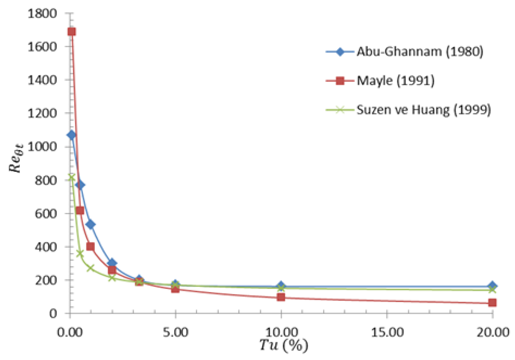
Abu-Ghannam and Shaw (1980) proposed a correlation between the Reynolds number of the transition to turbulence and the inlet turbulence intensity depending on the boundary layer momentum thickness. The correlation is expressed as follows:
The correlation suggested by Mayle (1991) is as follows:
Suzen and Huang (1999) included the following expression for the transition to turbulence in their numerical model:
The correlations expressing the turbulent transition Reynolds number according to the inlet turbulence intensity proposed by Abu-Ghannam and Shaw (1980), Mayle (1991) and Suzen and Huang (1999) mentioned above are compared in Figure 1.
Taghavi-Zenous et al. (2008) experimentally investigated the laminar to turbulent flow on a flat plate at different inlet turbulence intensities. The measurements were taken with a hot wire velocimetry in the range of 1.5-4.4% inlet turbulence intensity. They stated that with the increase in inlet turbulence intensity, the transition region becomes smaller and regresses towards lower Reynolds numbers and they derived an empirical expression for the turbulent transition Reynolds number depending on the inlet turbulence intensity as follows:
where: : 3346, 879.9, 419,5; : -0.3656, -0.8927, -12.93; : 0.2825, 1.782, 18.29
Figure 1.
Relationship between the Re number and the inlet turbulence intensity (Tu) at the transition to turbulence defined by the boundary layer thickness.
Figure 1.
Relationship between the Re number and the inlet turbulence intensity (Tu) at the transition to turbulence defined by the boundary layer thickness.
Sugawara et al. (1988) experimentally investigated the effect of turbulence intensity created by turbulent grids on heat transfer and flow characteristics. They stated that with the increase in inlet turbulence intensity, the Reynolds number from laminar to turbulent decreases and heat transfer increases, the flow in the laminar region is not affected by the inlet turbulence intensity, and the increase in Nu number is faster at high inlet turbulence intensity levels.
Peneau et al. (2004) investigated the effects of inlet turbulence intensity on the developing boundary layer on a plane plate using the LES (Large Eddy Simulation) turbulence model. They obtained results for different inlet turbulence intensities and compared them with experimental results. They stated that the LES turbulence model is suitable for investigating the effect of inlet turbulence intensity.
Langtry (2006) in his doctoral study modified the SST turbulence model for unstructured mesh structures and presented a correlation-based turbulence model using local variables that can solve the turbulence transition region more accurately. This model was soon included in the ANSYS CFX commercial CFD code. Langtry conducted validation studies on flat plates, helicopter aerodynamics, aircraft wing aerodynamics, and turbine blade aerodynamics in his doctoral study, and demonstrated that this model was more successful than Menter's SST model in the transition region. After this turbulence transition model was integrated into the ANSYS CFX code under the name Gamma-Theta, it was integrated into the other most well-known CFD codes in the market, ANSYS Fluent and Star CD, and became the most widely used turbulence model in the industry for solving the transition region. In the literature, the Gamma-Theta model has been used and validated in studies numerically examining the transition region (Bochon et al., 2008, Piotrowsky et al., 2008, Suluksna and Juntasaro, 2008).
Bochon et al. (2008) stated that the turbulence model that best solves the conjugate heat transfer in the transition region from laminar flow to turbulence is Gamma-Theta and that it is possible to obtain successful results by modifying other 2-equation models like Gamma-Theta.
Piotrowsky et al. (2008) studied the Gamma-Theta transition turbulence model on a plane plate and N3-60_04 turbine airfoil. As a result of the study, they stated that the Gamma-Theta turbulence model is in good agreement with the experimental results and can solve the transition to bypass and wake-induced turbulence very well.
Suluksna and Juntasaro (2008) studied to determine the effects of inlet turbulence intensity and pressure gradient on the transition region flow characteristics numerically using the Gamma-Theta model. They stated that the critical Re number changes only with the turbulence intensity, and that the pressure gradient does not affect the critical Re number much in zero pressure gradient and favorable pressure gradient flows, and the pressure gradient effect can be neglected.
Incropera and DeWitt (2003) mentioned in the literature that the inlet turbulence intensity and surface roughness affect the results up to 25% in forced convection.
Various studies on boundary layer transition are ongoing. A solver for boundary layer transition was developed by Bhushan and Walters (2014). Fabrizio (2014) investigated the critical phenomena in laminar-turbulent transition with a mean field model. A new turbulence model for modeling the turbulent transition according to mechanical priorities was proposed by Vizinho et al. (2015). The effects of wall heating on the boundary layer transition on a flat plate were investigated numerically by Subaşı and Güneş (2015). An evaluation of Reynolds Averaged Navier-Stokes (RANS Reynolds Averaged Navşer-Stokes) turbulence models in convective heat transfer was made numerically by Abdollahzadeh et al. (2017). A new laminar kinetic energy model for the prediction of pre-transition velocity fluctuations and boundary layer transition was presented by Medina et al. (2018). Lienhard (2020) proposed a correlation for heat transfer in plane plate boundary layers under laminar, transitional and turbulent flow conditions.
As can be understood from the above studies, the findings in some studies contradict each other and since the effect of external turbulence on the flat plate is encountered in important application areas, studies on this subject are needed. Since the flow on the flat plate is frequently encountered in engineering problems, it is important to develop basic flow equations such as boundary layer for flow on the flat plate, to control the boundary layer and to examine the transition to turbulence. In this study, the effects of the inlet turbulence level on the zero pressure gradient flow on the flat plate based on the ERCOFTAC T3A test setup were investigated by comparing various turbulence models and it was determined that the Gamma-Theta (GT) model was the most suitable model. Then, using this model, the effect of turbulence intensity on the friction coefficient (Cf) was calculated numerically by keeping the integral length scale constant and the results were given in comparison with the experimental results.
2. Materials and Methods
In this study, Computational Fluid Dynamics (CFD) method is used to investigate the effect of inlet turbulence intensity on the friction coefficient for the zero pressure gradient (ZPG) flow, and for this purpose, conservation equations, namely continuity, momentum and turbulence model equations are solved under specified boundary conditions using ANSYS CFX commercial code. If the standard deviation divided by the mean velocity (), the turbulence intensityt, Tu is obtained:
where the velocity fluctuations, , are in the main direction of the flow. The turbulence length scale is considered as the sum of the integral length scale and the micro scale. Std. k-ε, RNG k-ε, std. k-ω, SST k-ω, and Gamma-Theta (GT) have been used and compared. Gamma-Theta turbulence model is a turbulence model that solves two separate transport equations for the transition criterion and “intermittency” based on the Reynolds number defined according to the momentum thickness, thus solving the transition region much more precisely. The empirical correlation it uses (Langtry and Menter 2005) is designed to capture the bypass transition even at low inlet turbulence intensities. It is used with the SST turbulence model in ANSYS CFX. Since all turbulence models are solved using their standard forms and recommended turbulence coefficients in the program, detailed information about the turbulence models and coefficients used can be found in the work of Erşan (2012) and in the modeling manual of the program (ANSYS CFX R13, 2010). ANSYS CFX includes a powerful pre- and post-processing interface and an advanced finite volume solver. ANSYS CFX solver has proven its reliability in terms of the results it has given both in the industry and in the literature. Stable results can be obtained during the solution thanks to its coupled solver.
2.1. Geometrical Model and Boundary Conditions
In the flat plate calculations, the computational domain of H = 0.26 m L = 2 m, shown in Figure 2 below, was used. This geometry was modeled under the same conditions, taking the ERCOFTAC T3A experimental setup as a reference (ERCOFTAC).
Figure 2.
Computational domain for flat plate.

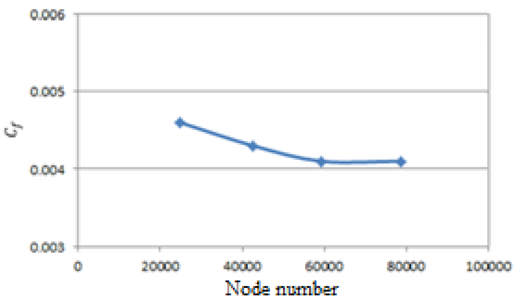
2.2. Mesh Independency Study
In the computations, the mesh-independent solution was investigated for four different network structures. The mesh-independent solution was obtained in the 4th mesh structure, and the computations were repeated with this mesh structure. The mesh-independent solution was obtained in the mesh structure with 60000 nodes. Four different mesh results are shown in Figure 3.
Figure 3.
Mesh independency study.
The computational domain seen above is divided into meshes with high-quality hexahedral solution elements, as seen below in Figure 4. A total of 135610 nodes were used. Dense elements were used at the entrance and near the wall.
Figure 4.
Mesh structure (135610 nodes).
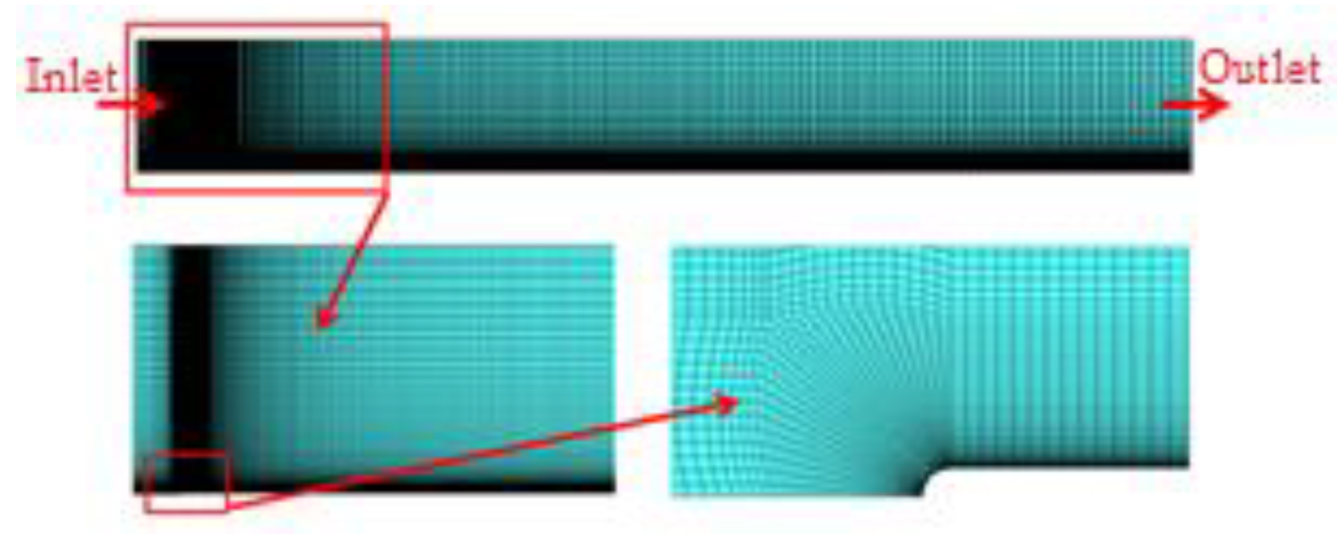
The computational domain has a 0.26 m in height and 2 m in length. A no-slip condition was defined at the lower plate to represent viscous flow over a flat plate. A frictionless wall boundary condition was defined at the upper plate. At the outlet, the pressure was defined as zero. Uniform inlet velocity of 5.3 m/s was defined at the inlet. These boundary conditions were used to represent the ERCOFTAC T3A test case.
2.3. Thermophysical Properties
The thermophysical properties of air have been considered at the inlet temperature, and are given in Table 1 below (Incropera and DeWitt, 2003).

Table 1.
Thermophysical properties of air.
| Density | 1,116 kg/m3 |
| Viscosity | 1,725 Pa.s |
| Conductivity | 0,02428 W/mK |
| Specific heat | 1003,8 J/kgK |
3. Results and Discussion
Laminar and turbulent numerical solutions for the ERCOFTAC T3A experimental test case on a flat plate are given and discussed in Figure 5 below.
Figure 5.
Comparison of Gamma-Theta (GT), Std. k-ɛ, RNG k-ɛ, Std. k-ω and SST k-ω turbulence models (This study).
Figure 5.
Comparison of Gamma-Theta (GT), Std. k-ɛ, RNG k-ɛ, Std. k-ω and SST k-ω turbulence models (This study).

When defining the Reynolds number in the flow on a flat plate, the characteristic length is used as the length in the flow direction. In Figure 5, from the experimental results, we see that the transition to turbulence begins at a local Re number of approximately 140000 in the flow and that the flow becomes fully turbulent at a local Re number of approximately 270000.
In Figure 5, it is seen that the laminar numerical solution gives results that are inconsistent with the experimental data, as expected, in the turbulent transition and turbulent flow regions. It is seen that the results obtained using the Std. k-ɛ, Std. k-ω, SST k- ω, and RNG k-ɛ turbulence models are also inconsistent in the laminar and turbulent transition regions, as expected. As can be seen in Figure 5, the solutions obtained with the Gamma-Theta-SST turbulent transition model are in agreement with the experimental results, unlike the other models, in the laminar, turbulent transition, and turbulent flow regions.
The above results show that the Gamma-Theta model is a suitable model for solving laminar, turbulent transition and turbulent regions in flat plate flow. However, although the compatibility with the experimental results in the turbulent transition region is not as good as in the laminar and turbulent regions, it can be said that it is at a quite acceptable level when the complexity of the flow in the transition region and the fact that other turbulence models cannot capture this region at all are taken into account. In the transition region, the Gamma-Theta model starts the transition earlier than the experimental data and completes the transition a little earlier. The friction coefficient is estimated at most 40% higher than the experimental results in this region. These results are for the ERCOFTAC T3A inlet turbulence intensity Tu=3.3 experimental case, and the turbulence length scale is not specified in this experimental case and the length scale is taken as LS=0.026 m in the calculations in this study. A certain part of the approximately 40% deviation from the experimental results in this region can be attributed to this.
When we inspect Figure 5, if the flow were completely turbulent (Rex > 270000), it is seen that the Gamma-Theta model is the most suitable turbulence model, and the model with the same suitability as this model is the Std. k-ω model. The other most suitable models are the SST- k-ω, Std. k-ɛ and RNG k-ɛ models, respectively. However, although the Gamma-Theta and Std. k-ω models are almost in agreement with the experimental data; the other models predict the friction coefficient below the experimental data at Reynolds numbers smaller than Rex = 440000, and it can be said that all of them show almost the same performance. Again, if the flow were completely laminar, it is seen from Figure 5 that the numerical solution is in very good agreement with the experimental data in the laminar region (0 < Re < 170000).
The Gamma-Theta turbulence model, which is the most suitable model to investigate the effect of inlet turbulence intensity, was selected and the effect of inlet turbulence intensity was investigated with this model. Five different calculations were made by keeping the turbulence length scale constant and changing the inlet turbulence intensity between 1% and 10%. The results are shown in Figure 6a together with the experimental and laminar numerical solution results. The turbulent transition regions are shown in Table 2. In addition, the results of the experimental study of Taghavi-Zenous et al. (2008) are given in Figure 6b for comparison. The experimental conditions of this experimental study are also shown in Table 3.
Table 2.
Transition regions of inlet turbulence intensity to turbulence on the plane plate in the Gamma-Theta turbulence model (This Study).
Table 2.
Transition regions of inlet turbulence intensity to turbulence on the plane plate in the Gamma-Theta turbulence model (This Study).
| Tu (%) | LS (m) | Inlet Velocity (m/s) | Laminar Region |
Transition Region of Turbulence | Turbulent Region |
|---|---|---|---|---|---|
| 1 | 0.026 | 5.3 | 0 < Re < ∞ | - | - |
| 2 | 0.026 | 5.3 | Re < 280000 | 280000 < Re < 400000 | Re > 400000 |
| 3.3 | 0.026 | 5.3 | Re < 115000 | 115000 < Re < 260000 | Re > 260000 |
| 5 | 0.026 | 5.3 | Re < 60000 | 60000 < Re < 150000 | Re > 150000 |
| 10 | 0.026 | 5.3 | - | - | 0 < Re < ∞ |
Table 3.
Experimental conditions (Taghavi-Zenous vd., 2008).
| Deney Kodu | Tu (%) | LS (m) | Giriş Hızı (m/s) |
|---|---|---|---|
| ZPG-TA | 1.5 | 0.009 | 15.5 |
| ZPG-TB1 | 3.2 | 0.0105 | 12 |
| ZPG-TB2 | 3.3 | 0.011 | 15 |
| ZPG-TC1 | 4.3 | 0.0126 | 8.35 |
| ZPG-TC2 | 4.4 | 0.0129 | 10.5 |
Since the transition to turbulence in the flow occurs when the critical Re number is exceeded, the change in the turbulence transition region according to the Re number is given in Table 2 for different inlet turbulence intensities. As the inlet turbulence intensity increases, the transition to turbulence occurs at lower Re numbers. In the case where the inlet turbulence intensity is 1%, since the calculations are made in the range of 0 < Re < 700000 and the turbulence transition region is outside this range, the turbulence transition region could not be determined and is shown with a “-” in Table 2. In the case where the inlet turbulence intensity is 10%, the flow occurs directly as turbulent and this time there is no laminar and turbulent transition region, so it is shown with a “-” in Table 2.
Figure 6.
Cf results of Gamma-Theta (GT) turbulence model for different inlet turbulence intensities a) This study b) Taghavi-Zenous et al. (2008).
Figure 6.
Cf results of Gamma-Theta (GT) turbulence model for different inlet turbulence intensities a) This study b) Taghavi-Zenous et al. (2008).
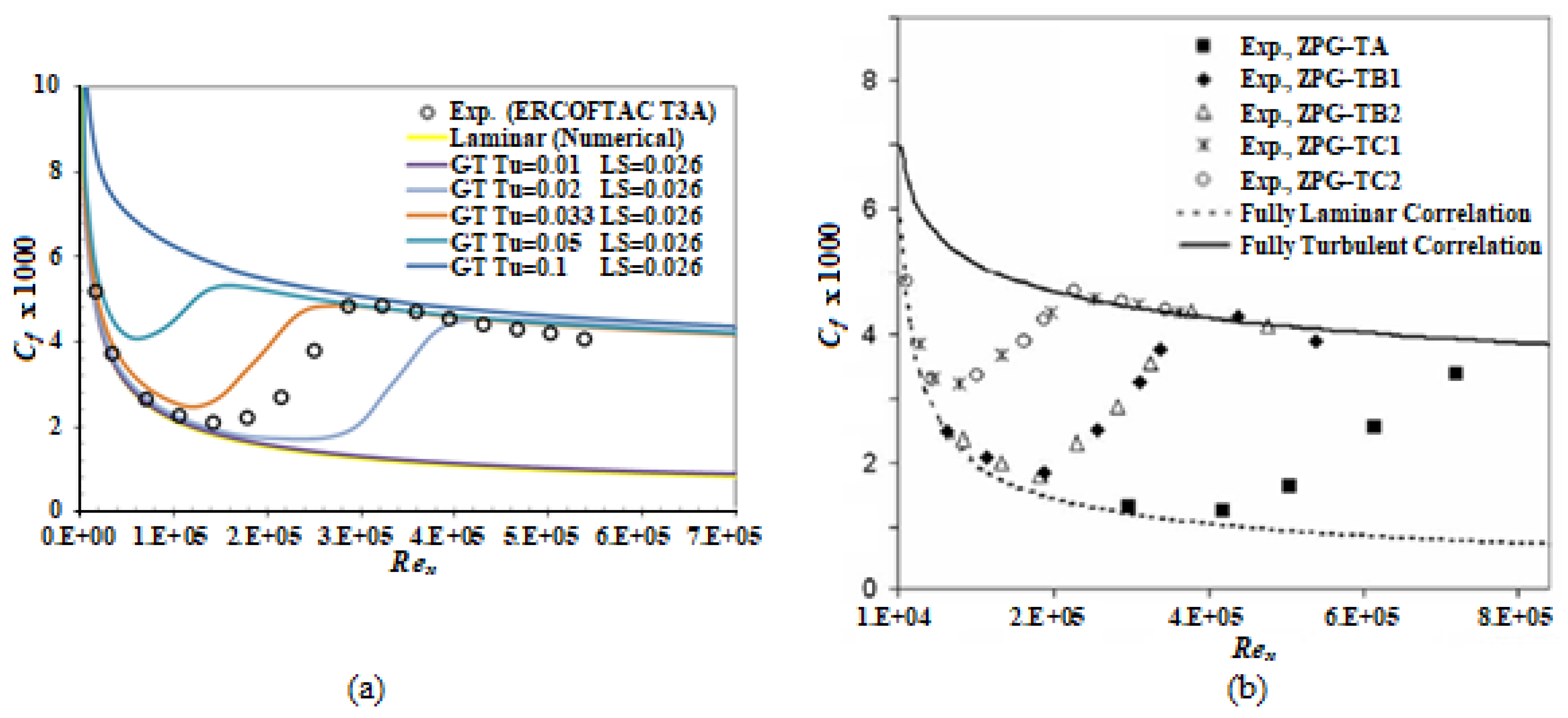
As seen in Figure 6a, with the increase in the inlet turbulence intensity, the transition to turbulence became easier and the laminar region shortened. Some results in Figure 6a are summarized in Table 2 and it can be seen that as the turbulence intensity increases, the transition region to turbulence narrows. This situation was also determined in the experimental study of Taghavi-Zenous et al. (2008).
When Figure 6a and Figure 6b are examined, it can be easily said that the numerical results in this study are consistent with the experimental results. Although the turbulence length scale was kept constant in this study, it should not be forgotten that this consistency should be evaluated qualitatively since it was not kept constant in the experimental study. Because, as stated in the studies of Hancock and Bradshaw (1983) and Iyer and Yavuzkurt (1999), where their studies were evaluated, the turbulence length scale is also effective on the boundary layer along with the turbulence intensity.
4. Conclusions
Two equation turbulence models of Std. k-ε, RNG k-ε, Std. k-ω ve SST k-ω have been compared with Gamma-Theta (GT) transitional model, and it has been found that Gamma Theta model is the most consistent model with the experimental values of the ERCOFTAC T3A test case.
It has also been observed that with the increase in the inlet turbulence intensity in the flow over the plane plate, the transition to turbulence becomes easier, the laminar region shortens and the transition region to turbulence narrows as the turbulence intensity increases. These results are also supported experimentally since they were also found in the experimental study of Taghavi-Zenous et al. (2008).
Transition from laminar to turbulence is shortened with increasing turbulence intensity by changing it from 0.01 to 0.1. The most suitable inlet turbulence intensity value with the experimental results of ERCOFTAC T3A test case is found as Tu=0.033.
Nomenclature
| ai, bi, ci | Constants in equation 4 |
| Cf | Friction coefficient |
| GT | Ghamma-Theta turbulence model |
| LS | Turbulent length scale |
| Reϴt | Transition to turbulence Reynolds number (Transitional Reynolds number) |
| Rex | Local Reynolds number |
| Tu | Turbulence intensity |
| ZPG | Zero pressure gradient |
Acknowledgments
Muhsine Saru is currently a doctoral student and acknowledges the financial support of YOK-Council of Higher Education in Turkey with grand number 100-2000.
Declaration of Competing Interest
The authors declare that they have no known competing financial interests or personal relationships that could have appeared to influence the work reported in this paper.
References
- Abdollahzadeh, M. , Esmaeilpour, M., Vizinho, R., Younesi, A., & Pascoa, J.C. Assessment of RANS turbulence models for numerical study of laminar-turbulent transition in convection heat transfer. Int. J. Heat Mass Transf. 2017, 115, 1288–1308. [Google Scholar]
- Abu-Ghannam, B. & Shaw, R. Natural transition of boundary layers - the effects of turbulence, pressure gradient and flow history. J. Mech. Eng. Sci. 1980, 22, 213–228. [Google Scholar]
- ANSYS CFX R13 Modelling Guide (2010).
- Blair, M.F. Influence of free-stream turbulence on turbulent boundary layer heat transfer and mean profile development, part 1-experimental data. J. Heat Transf.-Trans. ASME 1983, 105, 33–40. [Google Scholar] [CrossRef]
- Blair, M.F. Influence of free-stream turbulence on turbulent boundary layer heat transfer and mean profile development, Part II - Analysis of results. J. Heat Transf.-Trans. ASME 1980, 105, 41–47. [Google Scholar] [CrossRef]
- Bochon, K. , Wroblewski, W., & Dykas, S. Modelling of influence of turbulent transition on heat transfer conditions. Task Q. 2008, 12, 173–184. [Google Scholar]
- Bhushan, S. , & Walters, D.K. Development of Parallel Pseudo-Spectral Solver Using Influence Matrix Method and Application to Boundary Layer Transition. Eng. Appl. Comput. Fluid Mech. 2014, 8, 158–177. [Google Scholar]
- Büyüktür, A.R. , Kestin, J., & Maeder, P.F. Influence of combined pressure gradient and turbulence on the transfer of heat from a plate. Int. J. Heat Mass Transf. 1964, 7, 1175–1184. [Google Scholar]
- Emmons, H.W. The laminar-turbulent transition in a boundary layer – part1. J. Aeronaut. Sci. 1951, 18, 490–498. [Google Scholar] [CrossRef]
- Erşan, H.A. (2012). Numerical Investigation of the Effects of the Outer Turbulence in Fluid Flow and Heat Transfer Characteristics. M.Sc. Thesis, School of Natural and Applied Sciences, Mechanical Engineering Department, Uludag University.
- Fabrizio, M. Critical Phenomena in laminar-turbulence transitions by a mean field model. Meccanica 2014, 49, 2079–2086. [Google Scholar] [CrossRef]
- Hancock, P.E. , & Bradshaw, P. The effect of free-stream turbulence on turbulent boundary layers. J. Fluids Eng.-Trans. ASME 1983, 105, 284–289. [Google Scholar]
- Incropera, F.P. , & DeWitt, D.P. (2003). Fundamentals of Heat and Mass Transfer. Wiley.
- Iyer, G.R. , & Yavuzkurt, S. Comparison of low Reynolds number ke models in simulation of momentum and heat transport under high free stream turbulence. Int. J. Heat Mass Transf. 1999, 42, 723–737. [Google Scholar]
- Kestin, J. , Maeder, P.F., & Wang, H.E. Influence of turbulence on the transfer of heat from plates with and without a pressure gradient. Int. J. Heat Mass Transf. 1961, 3, 133–154. [Google Scholar]
- Langtry, R.B. (2006). A Correlation Based Transition Model Using Local Variables for Unstuctured Parallelized CFD Codes [Doctoral Dissertation, Universitat Stuttgart].
- Langtry, R. B. , Menter, M.R., 2005, Transitional Modeling of General CFD Applications in Aeronautics, 43rd AIAA Aerospace Sciences Meeting and Exhibit, Reno, Nevada. AIAA Paper 2005-522.
- Lienhard, J.H. , V (2020). Journal of Heat Transfer-Transactions of the ASME, 142(June), 061805.1-14.
- Maciejewski, P.K. , & Moffat, R.J. Heat transfer with very high free stream turbulence: part 1-Experimental data. J. Heat Transf.-Trans. ASME 1992, 114, 827–833. [Google Scholar]
- Maciejewski, P.K. , & Moffat, R.J. Heat transfer with very high free stream turbulence: part 2-Analysis of results. J. Heat Transf.-Trans. ASME 1992, 114, 834–839. [Google Scholar]
- Mayle, R.E. The role of laminar-turbulent transition in gas turbine engines. J. Turbomach.-Trans. ASME 1991, 113, 509–536. [Google Scholar] [CrossRef]
- Medina, H. , Beechook, A., Fadhila, H., Aleksandrova, S., & Benjamin, S. A novel laminar kinetic energy model for the prediction of pretransitional velocity fluctuations and boundary layer transition. Int. J. Heat Fluid Flow 2018, 69, 150–163. [Google Scholar]
- Peneau, F.E. , Boisson, H.C., Kondjoyan, A., & Djilali, N. Structure of a flat plate boundary layer subjected to free stream turbulence. Int. J. Comput. Fluid Dyn. 2004, 18, 175–188. [Google Scholar]
- Piotrowski, W. , Elsner, W., & Drobniak, S. Transition prediction on turbine blade profile with intermittency transport equation. J. Turbomach.-Trans. ASME 2008, 132, 011020. [Google Scholar]
- Saric, W.F. (1992). Special Course on Skin Friction Drag Reduction (Reduction de Trainee de Frottement) AGARD-R-786 [Laminar-turbulent transition:Fundamentals]. NATO.
- Schlichting, H. (1979). Boundary Layer Theory. McGraw-Hill, New York.
- Simonich, J.C. , & Bradshaw, P. Effect of free-stream turbulence on heat transfer through a turbulent boundary layer. J. Heat Transf.-Trans. ASME 1978, 100, 671–677. [Google Scholar]
- Subaşı, A. , & Güneş, H. Effects of wall heating on boundary layer transition over a flat plate. J. Therm. Sci. Technol. 2015, 35, 59–68. [Google Scholar]
- Sugawara, S. , Sato, T., Komatsu, H., & Osaka, H. Effect of Free Stream Turbulence on Flat Plate Heat Transfer. Int. J. Heat Mass Transf. 1988, 31, 5–12. [Google Scholar]
- Suluksna, K. , & Juntasaro, E. Assessment of intermittency transport equations for modeling transition in boundary layers subjected to freestream turbulence. Int. J. Heat Fluid Flow 2008, 29, 48–61. [Google Scholar]
- Suzen, Y. , Huang, P.G. (1999). Special Course on Skin Friction Drag Reduction (Reduction de Trainee de Frottement) AGARD-R-786 [Modelling of flow transition: Fundamentals]. NATO.
- Taghavi-Zenous, R. , Salari, M., Tabar, M.M., & Omidi, E. Hot-wire anemometry of transitional boundary layers exposed to different freestream turbulence intensities. Proc. Inst. Mech. Eng. Part G J. Aerosp. Eng. 2008, 222, 347–356. [Google Scholar]
- Wisler, D.C. (1998). Minnowbrook II1997 Workshop on Boundary Layer Transition in Turbomachine [The Technical and Economic Relevance of Understanding Boundary Layer Transition in Gas Turbine Engines,]. NASA CP-1998-206958.
- Vizinho, R. , Pascoa, J., & Silvestre, M. Turbulent transition modeling through mechanical considerations. Appl. Math. Comput. 2015, 269, 308–325. [Google Scholar]
Disclaimer/Publisher’s Note: The statements, opinions and data contained in all publications are solely those of the individual author(s) and contributor(s) and not of MDPI and/or the editor(s). MDPI and/or the editor(s) disclaim responsibility for any injury to people or property resulting from any ideas, methods, instructions or products referred to in the content. |
© 2025 by the authors. Licensee MDPI, Basel, Switzerland. This article is an open access article distributed under the terms and conditions of the Creative Commons Attribution (CC BY) license (https://creativecommons.org/licenses/by/4.0/).
Copyright: This open access article is published under a Creative Commons CC BY 4.0 license, which permit the free download, distribution, and reuse, provided that the author and preprint are cited in any reuse.


