
Submitted:
20 March 2025
Posted:
21 March 2025
You are already at the latest version
Abstract
This paper describes methods for optimal filtering of random signals that involve large matrices. We develop a procedure that allows us to significantly decrease the computational load needed to numerically realize the associated filter and increase the associated accuracy. The procedure is based on the reduction of a large covariance matrix to a collection of smaller matrices. It is done in such a way that the filter equation with large matrices is equivalently represented by a set of equations with smaller matrices. The filter Fp we develop is represented by Fp(v1,…vp)=∑j=1pMjvj and minimizes the associated error over all matrices M1,…,Mp. As a result, the proposed optimal filter has two degrees of freedom to increase the associated accuracy. They are associated, first, with the optimal determination of matrices M1,…,Mp and second, with the increase in the number p of components in the filter Fp. The error analysis and results of numerical simulations are provided.
Keywords:
large covariance matrices
; least squares linear estimate
; singular value decomposition
; error minimization
1. Introduction
1.1. Preliminaries
Although there is an extensive literature on studying methods of filtering of random signals, the problem we consider seems to be different from the known ones. The objective of this paper is to formulate and solve this problem under scenarios which relate to a reduction of computation complexity, for the case of large covariance matrices, and an increase in the filtering accuracy.
Let be a set of outcomes in probability space for which is a –algebra of measurable subsets of and is an associated probability measure. Let be a signal of interest and be an observable signal.. Here is the space of square-integrable functions defined on with values in , i.e., such that
Further, let us write where , for . We assume without loss of generality that all random vectors are of the zero mean. Let us denote
where is the covariance matrix formed from and .
Let filter F be represented by where . Note that each matrix defines a bounded linear transformation . It is customary to write M rather then since , for each .
The known problem of finding optimal filter F is formulated as follows. Given large covariance matrices and , find M that solves
1.2. Motivations
In 3, M contains entries. In other words, the filter defined by 3 contains parameters to optimize the associated accuracy.
Motivation 1: Increase in accuracy. Since M in 3 is optimal there is no other linear filter that can provide a better associated accuracy. At the same time, it may happen that the accuracy is not satisfactory. Then a logical way to increase the accuracy is an increase in the number of parameters to optimize. Since m is fixed then only n can be varied; n can be increased to, say, q where , if is replaced with another vector which is unknown. In this case, we need to determine both M and . In particular, can be represented as where, for and . Then the associated filter is represented by the equation
where, for . We call p the degree of filter .
Therefore, the preliminary statement of the problem considered here and in [6] is as follows. Given and , find and that solve
Note, since and are given then, for , and are known as blocks of and .
Motivation 2: Decrease in computational load. In 2 and 3, dimensions of and , m and n, respectively, can be very large. In a number of important applied problems, such as those in biology, ecology, finance, sociology and medicine (see e.g., [7,8]), and greater. For example, measurements of gene expression can contain tens of hundreds of samples. Each sample can contain tens of thousands of genes. As a result, in such cases, associated covariance matrices matrices in 3 are very large. Further, in (4) and (5), dimension of might be of the same order as that of observable signal . For instance, one of can be equal to . Based on 2–(5), it is natural to predict that a solution of problem (5) contains pseudo-inverse and pseudo-inverse . It is indeed so, as shown in Section 4.1.6 and [6]. Matrices and are usually larger than . Then computation of a large pseudo-inverse matrix leads to a quite slow computing procedure up to the cases when the computer runs out of computer memory. In particular, the associated well-known phenomenon of the “curse of dimensionality” [9] states that many problems become exponentially difficult in high dimensions.
Of course, in the case of high dimensional signals, some well known dimensionality reduction techniques can be used (as those, for example, in [2,3,5]) as an intermediate step for the filtering. At the same time, those techniques also involve large pseudo-inverse covariance matrices of the same size as that in 3. Additionally, in applying the dimensionality reduction procedure, intrinsic associated errors appear. The errors may involve, in particular, an undesirable distortion of the data. Thus, an application of the dimensionality reduction techniques to the problem under consideration does not allow us to avoid a computation of large pseudo-inverse covariance matrices. Therefore, we wish to develop techniques that reduce computation of large pseudo-inverses and without involving any additional associated error.
The following example illustrates Motivation 2. Simulations in this example and also in 2 of Section 4.1.7 were run on a Dell Latitude 7400 Business Laptop (manufactured in 2020).
Example 1.
Let be a matrix whose entries are normally distributed with mean 0 and variance 1. In Table 1, we provide the time (in seconds) needed forMatlabto compute matrix for different values of q.
We observe that computation of, e.g., pseudo-inverse matrix requires 63 seconds while computation of the five pseudo-inverse matrices of sizes requires about seconds. Thus, a procedure that would allow us to reduce the computation of to a computation of, say, five pseudo-inverse matrices of sizes would be faster. At the same time, such a procedure would additionally contain associated matrix multiplications which are time consuming as well. This observation is further elaborated in Section 4.1.2 and 2 of Section 4.1.7.
2. Statement of the Problem
The solution of the problem in (5) is divided into two parts. In this paper, we consider the first part of the solution. It mainly concerns a technique for the decrease in a computational load associated with computation of . The second part of the solution of problem (5) is considered in [6]. It represents an extension of the technique considered here to the solution of the original problem in (5). More precisely, here, we consider
In terms of notation (4), the known minimal Frobenius norm solution of (6) is given by (see, e.g., [1,2,3,4,5])
As mentioned in Section 1.2, in (7) (and in (8) below), matrix might be very large. Then the pseudo-inverse may be difficult to compute. In this case, formula in (7) is not useful in practice.
Therefore, the problem is as follows. Given large and , find a computational procedure for solving (6) which significantly decreases the computational complexity for the evaluation compared to that needed by the filter represented by (7).
While problem (6) arises in the solution provided in [6] it is also important in its own right. In particular, if where, for , and , then (6) represents the problem of finding the optimal multi-input multi-output (MIMO) filter. In this case, and , for , are an input signal and output signal, respectively.
The problem in (6) can also be interpreted as the system identification problem [10,11,12,13]. In this case, are the inputs of the system, is the input-output map of the system, and is the system output. For example, in environmental monitoring, may represent random data coming from nodes measuring temperature, light or pressure variations, and may represent a random signal obtained after a merging of the received data in order to estimate required data parameters within a prescribed accuracy. Similar scenarios occur, e.g., in target localization and tracking [14].
As mentioned above, in all problems considered in this paper, covariance matrices are assumed to be known. This assumption is a well-known and significant limitation in problems dealing with the optimal filtering of random signals. See [15,16,17,18] in this regard. The covariances can be estimated in various ways and particular techniques are given in many papers. We cite [19,20,21,22,23,24] as the examples. Estimation of covariance matrices is an important problem which is not considered in this paper.
3. Contribution and Novelty
The main conceptual novelty of the approach developed in this paper is in the technique that allows us to decrease the computational load needed for the numerical realization of the proposed filter. The procedure is based on the reduction of a large matrix to a collection of smaller matrices. It is done so that the filter equation with large matrices is equivalently represented by the set of equations with smaller matrices. As a result, as shown in Section 4.1.7, the proposed p-th degree filter requires computation of p pseudo-inverse matrices with sizes smaller that the size of the large matrix . In this regard, see Section 4.1.2, and 1 and 2, for more details. The associated Matlab code is given in Section 4.1.7.
In 2, 3 and 4, we also show that the accuracy of the proposed filter increases with increases in the degree of the filter. Details are provided in Section 4.1 and more specifically, in Section 4.1.2. In particular, the algorithm for the optimal determination of is given in Section 4.1.7. Note that the algorithm is easy to implement numerically. The error analysis associated with the filter under consideration is provided in Section 4.1.3, Section 4.1.5 and Section 4.1.8.
Remark 1.
Note that for every outcome , realizations and of signals and , respectively, occur with certain probabilities. Thus, random signals , for and are associated with infinite sets of realizations and , respectively. For different ω, the values , for and are, in general, different, and in many cases will span the entire spaces and , respectively. Therefore, for each and , for , filter given by (4) can be interpreted as map where probabilities are assigned to each column of and . Importantly, the filter is invariant with respect to outcome , and therefore, is the same for all and with different outcomes .
4. Solution of the Problem
We wish that in (5) and (6), would never been the zero vector. To this end, we need to extend the known definition of the linear independence of vectors as follows.
Let be some matrices. For , let be a null space of matrix .
A linear combination in the generalized sense of vectors is a vector
We say that the linear combination in generalized sense is non-trivial if , for at least one of Note that if where is the zero matrix, then it is still, of course, possible that . Therefore, condition is more general than condition .
Definition 1.
Random vectors are called linearly independent in the generalized sense if there is no non-trivial linear combination in the generalized sense of these vectors equal to the zero vector; in other words, if
for almost all , implies that , for each , and almost all .
All random vectors considered below are assumed to be linearly independent in the generalized sense.
4.1. Solution of Problem in (6)
Here, we exploit the specific structure of the original system (8) to develop a special block elimination procedure that allows us to reduce the original system of equations (8) to a collection of independent smaller subsystems. Their solution implies less computational load than that needed for (7).
We provide a specific solution of equation (10) in the following way. First, in Section 4.1.1, a generic basis for the solution is given. In Section 4.1.4, the solution of equation (10) is considered for . This is a preliminary step for the solution of equation (10) for an arbitrary p which is provided in Section 4.1.6.
4.1.1. Generic Basis for the Solution of Problem (8): Case in (10). Second Degree Filter
To provide a generic basis for the solution of equation (10), let us consider the case in (4) and (6), i.e., the second degree filter. Then (10) becomes
We denote
Proof.
The latter implies 14. ▪
Remark 2.
The above proof is based on equation (15) which implies the equivalence of equations (11) and 14. In turn, (1) allows us to equivalently obtain 14 as follows. Let us multiply (11) from the right by . Then
i.e.,
Theorem 1.
For the minimal Frobenius norm solution of problem (8) is represented by
Proof.
It follows from (21) that the second degree filter requires computation of two pseudo-inverse matrices, and , of sizes that are smaller than the size of (if, of course, and ).
4.1.2. Decrease in Computational Load
Here, we wish to compare the computational load needed for a numerical realization of the second degree filter given, for , by (4) and (21), and that of the filter represented by (7).
By [25] (p. 254), the product of and matrices requires, for large and q, flops. For large q, the Golub-Reinsch SVD used for computation of the matrix pseudo-inverse requires flops (see [25], p. 254).
In (12), for , the evaluation of implies the evaluation of , matrix multiplications in and matrix subtraction. These operations require flops, flops and flops, respectively. Similarly, computation of requires flops. In (21), computation of and imply flops and flops, respectively.
Let us denote by a number of flops required to compute an operation A. In total, the second degree filter requires flops where
Thus, the number of flops needed for the numerical realization of the second degree filter is equal to .
The computational load required by the filter given by (7) is flops. It is customary to choose . In this case, clearly, . In particular, if then the latter inequality becomes That is, for sufficiently large m and q, the proposed second degree filter requires, roughly, up to times less flops than that by the filter given by (7). In simulations by Matlab provided in 2 below, the second degree filter takes about two times less seconds than the filter given by (7). A command that would allow us to compute a number of flops is not available in Matlab.
In the following Section 4.1.4 and Section 4.1.6, the procedure described in Section 4.1.1 is extended to the case of the filter of higher degrees. For given q, this will imply, obviously, smaller sizes of blocks of matrices and than those for the second degree filter, and as a result, a further decrease in the associated computational load.
4.1.3. Error Associated with the Second Degree Filter Determined by (4)
Now, we wish to show that the error associated with the second degree filter determined, for , by (4) and (21) is less than the error associated with the filter determined by 3.
Let us denote
The Frobenius norm of matrix M is denoted by .
Theorem 2.
Let and be such that
where and . Then
Proof.
It is known (see, for example, [1,2,3,4,5]) that, for M determined by 3, and for and determined by (21),
where and, bearing in mind (2), . Therefore, by (21),
Then
At the same time,
Remark 3.
The condition in (23) can practically be satisfied by, in particular, a suitable choice of and , and/or their dimensions. The following 1 demonstrates such a particular choice of .
Corollary 1.
Let and be a nonzero signal. Then (24) is always true.
In general, the proposed solution of equation ((10)) is based on a combination of (1) and (2) with the extension of the idea of Gaussian elimination [25] to the case of matrices with specific blocks and . This allows us to build the special procedure considered below in Section 4.1.4 and Section 4.1.6.
4.1.4. Solution of Equation (10) for
To clarify the solution device of equation (10) for an arbitrary p, let us now consider a particular case with . The solution is based on the development of the procedure represented by (19) and (20).
For , equation (10) is as follows:
First, consider a reduction of (29) to the equation with the block-lower triangular matrix.
Step 1. By (13), for , . Define
Now, in (29), for and , update block-matrices and to and , respectively, so that
and
where , for and , and , for . Note that by (13).
Step 2. Set
By (13), . Taking the latter into account, update block-matrices and in the LHS of (31) and 31, for and , so that
and
where and .
As a result, we finally obtain the updated matrix equation with the block-lower triangular matrix
Solution of equation (34). Using a back substitution, equation (34) is represented by the three equations as follows:
where and are the original blocks in (29).
It follows from (35)–(37) that the solution of equation (10), for , is represented by the minimal Frobenius norm solutions to the problems
where and are solutions to the problems in (38) and (39), respectively. Matrices , for , that solve (38)-(40) are as follows:
Thus, the third degree filter requires computation of three pseudo-inverse matrices, , and .
4.1.5. Error Associated with the Third Degree Filter Determined by (41)–(43)
We wish to show that the error associated with the filter determined by (41)–(43), is less than that associated with the filter determined by 3, .
To this end, let us denote
where . As before, and .
Theorem 3.
Let , and be such that
Then
Proof.
Corollary 2.
If , and at least one of or is a nonzero vector then (46) is always true.
4.1.6. Solution of Equation (10) for Arbitrary p
Here, we extend the procedure considered in (Section 4.1.4) to the case of an arbitrary p. First, we reduce the equation in (10) to an equation with the block-lower triangular matrix. We do it by the following steps where each step is justified by an obvious extension of (1).
Step 1. First, in (10), for and , we wish to update blocks and to and , respectively. To this end, define
Bearing in mind that by (13), , for , we obtain
and
where, for and ,
and
Step 2. Now we wish to update blocks and , for and , of the matrices in the LHS of (49) and (50), respectively.
We continue this updating procedure up to the final Step . In Step , the following matrices are obtained:
and
4.1.7. Solution of Equation (10)
In (65)–(67), are solutions to the problems in (64)–(66), respectively. On the basis of [26], the minimal Frobenius norm solutions to (64)–(67) are given by
Thus, the p-th degree filter requires computation of p pseudo-inverse matrices, , , .
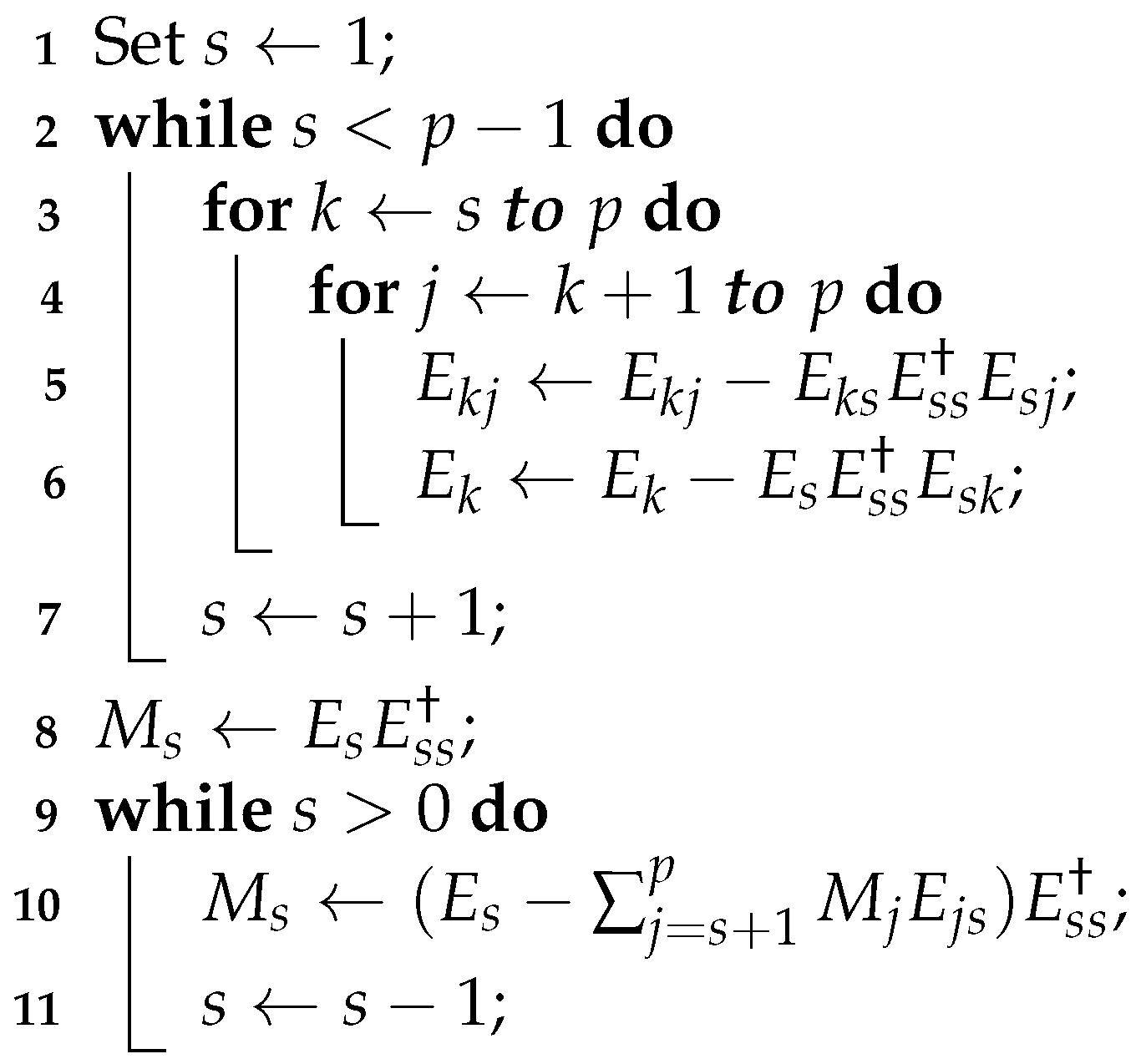
The algorithm that follows is based on formulas (51), (52), (55), (56), (61), (62) and (68)–(71).
| Algorithm 1: Solution of equation (10) |
|
Input: p, for , and for .
Output: for .
|
Note that the algorithm is quite simple. Its output is constructed from the successive computation of matrices and .
- In line 5, matrix is calculated as in (68).
Importantly, is the matrix with , therefore, it requires less computation than pseudo-inverse in (7).
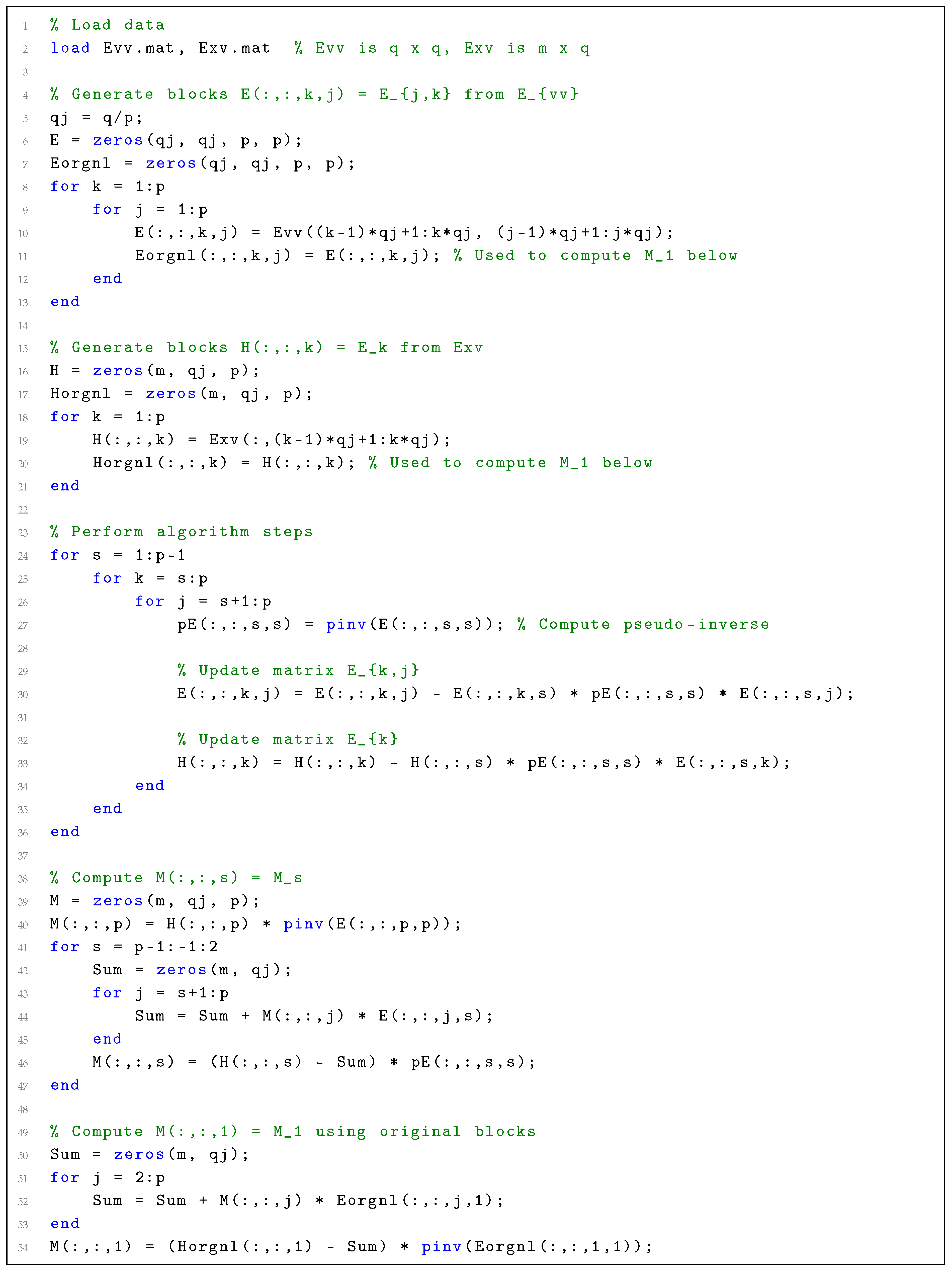
In the Matlab code below, are as above and Evv.mat, Exv.mat are files containing matrices and , respectively.
Listing 1. MATLAB Code for Solving Equation (10). |
 |
Example 2.
Here, we wish to numerically illustrate the above algorithm andMatlabcode. To this end, in equation (10), we consider matrices and whose entries are normally distributed with mean 0 and variance 1. We choose , , and , for .
In Table 2 and Figure 1, for , diagrams of the time needed by the above algorithm versus different values of dimension q are presented. Recall, the simulations carry out by the Dell Latitude 7400 Business Laptop (manufactured in 2020). The time decreases with the increase in p. In other words, the computational load needed for the numerical realization of the proposed p-th degree filer decreases with the increase in degree p. Note that the proposed p-th degree filter requires computation of p pseudo-inverse matrices and also matrix multiplications determined by the above algorithm. In particular, for and the proposed filter is around four times faster than the filter defined by (7).
4.1.8. The Error Associated with the Filter Represented by (4) and (68)–(71)
Let us denote by
the error associated with the filter determined by (4) and (68)–(71). We wish to analyze the error.
Theorem 4.
Let be a nonzero vector. Then the error decreases if the degree of the proposed filter p increases, i.e.,
In particular, if are such that
then is less than ϵ, the error associated with the filter given by (3),
Proof.
Remark 4.
Of course, in practice, the condition in (23) can easily be satisfied by a variation of the dimensions of vectors and/or by their choice. The following (3) illustrates this observation.
Corollary 3.
If and at least one of is not the zero vector then (76) is always true.
5. Conclusion
In a number of important applications, such as those in biology and medicine, associated random signals are high-dimensional. Therefore, covariance matrices formed from those signals are high-dimensional as well. Large matrices also appear because of the filter structure. As a result, the numerical realization of the filter that processes high-dimensional signals might be very time consuming, and in some cases run out of computer memory. In this paper, we have presented a method of optimal filter determination which targets the case of high-dimensional random signals. In particular, we have developed a procedure that significantly decreases the computational load needed to numerically realize the filter (see (Section 4.1.7) and (2)). The procedure is based on the reduction of the filter equation with large matrices to its equivalent representation by the set of equations with smaller matrices. The associated algorithm has been provided. The algorithm is easy to implement numerically. We have also shown that the filter accuracy is improved with an increase in filter degree, i.e. in the number of filter parameters (see (4)).
The provided results demonstrate that in high-dimensional random signal settings, a number of existing applications may benefit from using the proposed technique. The Matlab code is given in (Section 4.1.7). In [6], the technique provided here is extended to the case of filtering which is optimal with respect to minimization of both matrices and random vectors .
Author Contributions
Conceptualization, P.H, A.T. and P.S.Q.; methodology, P.H. and A.T.; software, A.T. and P.S.Q; validation, P.H. and A.T.; writing – original draft, A.T.; visualization, P.S.Q. All authors have read and agreed to the published version of the manuscript.
Funding
This research received no external funding.
Data Availability Statement
The raw data supporting the conclusions of this article will be made available by the authors on request.
Acknowledgments
This work was financially supported by Vicerrectoría de Investigación y Extensión from Instituto Tecnológico de Costa Rica (Research #1440054).
Conflicts of Interest
The authors declare no conflicts of interest.
References
- Fomin, V.N.; Ruzhansky, M.V. Abstract Optimal Linear Filtering. SIAM Journal on Control and Optimization 2000, 38, 1334–1352. [Google Scholar] [CrossRef]
- Hua, Y.; Nikpour, M.; Stoica, P. Optimal reduced-rank estimation and filtering. IEEE Transactions on Signal Processing 2001, 49, 457–469. [Google Scholar]
- Brillinger, D.R. Time Series: Data Analysis and Theory; 2001. [Google Scholar]
- Torokhti, A.; Howlett, P. An Optimal Filter of the Second Order. IEEE Transactions on Signal Processing 2001, 49, 1044–048. [Google Scholar] [CrossRef]
- Scharf, L. The SVD and reduced rank signal processing. Signal Processing 1991, 25, 113–133. [Google Scholar] [CrossRef]
- Howlett, P.; Torokhti, A.; Soto-Quiros, P. Decrease in computational load and increase in accuracy for filtering of random signals. Part II: Increase in accuracy. Signal Processing (submitted).
- Leclercq, M.; Vittrant, B.; Martin-Magniette, M.L.; Boyer, M.P.S.; Perin, O.; Bergeron, A.; Fradet, Y.; Droit, A. Large-Scale Automatic Feature Selection for Biomarker Discovery in High-Dimensional OMICs Data. Frontiers in Genetics 2019, 10. [Google Scholar] [CrossRef] [PubMed]
- Artoni, F.; Delorme, A.; Makeig, S. Applying dimension reduction to EEG data by Principal Component Analysis reduces the quality of its subsequent Independent Component decomposition. Neuroimage 2018, 175, 176–187. [Google Scholar] [CrossRef] [PubMed]
- Bellman, R.E. Dynamic Programming, 2 ed.; Courier Corporation, 2003. [Google Scholar]
- Stoica, P.; Jansson, M. MIMO system identification: State-space and subspace approximation versus transfer function and instrumental variables. IEEE Transactions on Signal Processing 2000, 48, 3087–3099. [Google Scholar] [CrossRef]
- Billings, S.A. Nonlinear System Identification - Narmax Methods in the Time, Frequency, and Spatio-temporal Domains; John Wiley and Sons, Ltd., 2013. [Google Scholar]
- Schoukens, M.; Tiels, K. Identification of Block-oriented Nonlinear Systems Starting from Linear Approximations: A Survey. Automatica 2017, 85, 272–292. [Google Scholar] [CrossRef]
- Howlett, P.G.; Torokhti, A.P.; Pearce, C.E.M. A Philosophy for the Modelling of Realistic Non-linear Systems. Processing of Amer. Math. Soc. 2003, 131, 353–363. [Google Scholar] [CrossRef]
- Li, D.; Wong, K.D.; Hu, Y.H.; Sayeed, A.M. Detection, classification, and tracking of targets. IEEE Signal Processing Mag. 2002, 19, 17–29. [Google Scholar]
- Mathews, V.J.; Sicuranza, G.L. Polynomial Signal Processing; John Willey & Sons, Inc.: New York, 2001. [Google Scholar]
- Marelli, D.E.; Fu, M. Distributed weighted least-squares estimation with fast convergence for large-scale systems. Automatica 2015, 51, 27–39. [Google Scholar] [CrossRef] [PubMed]
- Torokhti, A.P.; Howlett, P.G. Best Operator Approximation in Modelling of Nonlinear Systems. IEEE Trans. CAS. Part I, Fundamental theory and applications 2002, 49, 1792–1798. [Google Scholar]
- Torokhti, A.; Howlett, P. Best approximation of identity mapping: the case of variable memory. Journal of Approximation Theory 2006, 143, 111–123. [Google Scholar] [CrossRef]
- Perlovsky, L.; Marzetta, T. Estimating a covariance matrix from incomplete realizations of a random vector. IEEE Transactions on Signal Processing 1992, 40, 2097–2100. [Google Scholar] [CrossRef] [PubMed]
- Ledoit, O.; Wolf, M. A well-conditioned estimator for large-dimensional covariance matrices. Journal of Multivariate Analysis 2004, 88, 365–411. [Google Scholar] [CrossRef]
- Ledoit, O.; Wolf, M. Nonlinear shrinkage estimation of large-dimensional covariance matrices. The Annals of Statistics 2012, 40, 1024–1060. [Google Scholar] [CrossRef]
- Vershynin, R. How Close is the Sample Covariance Matrix to the Actual Covariance Matrix? J. Th. Prob. 2012, 25, 655–686. [Google Scholar] [CrossRef]
- Joong-Ho Won, Johan Lim, S.J.K.; Rajaratnam, B. Condition-number-regularized covariance estimation. Journal of the Royal Statistical Society: Series B) 2013, 75, 427–450. [CrossRef]
- Schneider, M.K.; Willsky, A.S. A Krylov Subspace Method for Covariance Approximation and Simulation of Random Processes and Fields. Multidimensional Systems and Signal Processing 2003, 14, 295–318. [Google Scholar] [CrossRef]
- Golub, G.; Van Loan, C. Matrix Computations, 4 ed.; Johns Hopkins Studies in the Mathematical Sciences, Johns Hopkins University Press, 2013. [Google Scholar]
- Friedland, S.; Torokhti, A. Generalized Rank-Constrained Matrix Approximations. SIAM Journal on Matrix Analysis and Applications 2007, 29, 656–659. [Google Scholar] [CrossRef]
Figure 1.
Time needed by the above algorithm, for , versus dimension q.
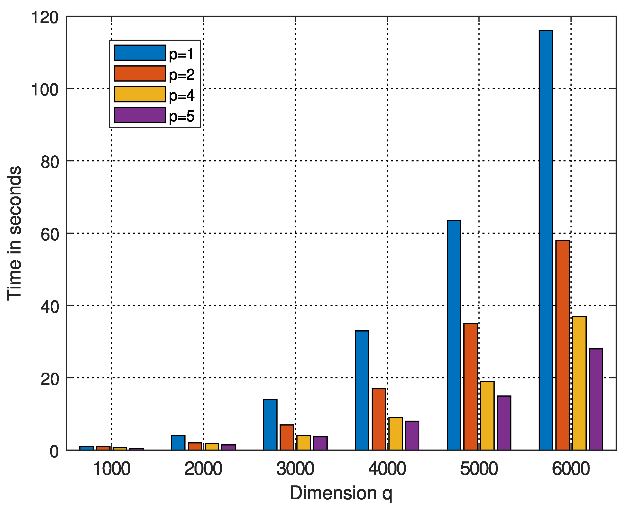

Table 1.
Time needed for Matlab to compute for different dimensions q.
| q | 500 | 1000 | 2000 | 3000 | 4000 | 5000 | 6000 |
|---|---|---|---|---|---|---|---|
| Time | 4 | 14 | 33 | 63 | 115 |
| Dimension q | ||||||
| 1000 | 2000 | 3000 | 4000 | 5000 | 6000 | |
| Time in seconds | ||||||
| 1 | 4 | 14 | 33 | 116 | ||
| 1 | 2 | 7 | 17 | 35 | 58 | |
| 4 | 9 | 19 | 37 | |||
| 8 | 15 | 28 | ||||
Disclaimer/Publisher’s Note: The statements, opinions and data contained in all publications are solely those of the individual author(s) and contributor(s) and not of MDPI and/or the editor(s). MDPI and/or the editor(s) disclaim responsibility for any injury to people or property resulting from any ideas, methods, instructions or products referred to in the content. |
© 2025 by the authors. Licensee MDPI, Basel, Switzerland. This article is an open access article distributed under the terms and conditions of the Creative Commons Attribution (CC BY) license (http://creativecommons.org/licenses/by/4.0/).
Copyright: This open access article is published under a Creative Commons CC BY 4.0 license, which permit the free download, distribution, and reuse, provided that the author and preprint are cited in any reuse.


