
Submitted:
18 March 2025
Posted:
19 March 2025
You are already at the latest version
Abstract
Real estate is crucial to the global economy, propelling economic and social development. This study examines the effects of dimensionality reduction through Recursive Feature Elimination (RFE), Random Forest (RF), and Boruta on real estate price prediction, as-sessing ensemble models like Bagging, Random Forest, Gradient Boosting, AdaBoost, Stacking, Voting, and Extra Trees. The findings indicate that the Stacking model achieved the best performance with an MAE of 14,092.30, an MSE of 5.34 × 10⁸, an RMSE of 23,104.19, and an R² of 0.9241, followed closely by Gradient Boosting (MAE = 14,536.52, R² = 0.9197). However, applying RFE for a variable reduction in Gradient Boosting led to a 16.9% increase in MAE and a 1.6% decrease in R². A similar trend was noted in Stacking, where the complete version had a 14.6% lower MAE. RF also displayed variable impacts: Gradient Boosting and Stacking saw MAE increases of 19.1% and 17.7%, respectively, whereas RF combined with AdaBoost enhanced performance with a 5.3% reduction in MAE. Boruta enabled the reduction of variables to 16 without significantly impacting ac-curacy; in Stacking, the MAE only increased by 9.8%, while R² decreased to 0.9082. Beyond accuracy, dimensionality reduction enhances computational efficiency, promoting scala-bility in real applications. Future research should investigate hyperparameter optimiza-tion and hybrid strategies to boost performance in complex settings.
Keywords:
Ensemble model
; machine learning
; prediction
; real estate
; regression
; dimensionality re-duction
; feature selection
; model optimization
1. Introduction
The real estate market represents an essential component of the global economy [1], substantially impacting macroeconomic and microeconomic dynamics [2,3]. The importance is evidenced by its ability to influence economic growth [4,5] , mainly through changes in real estate prices [2]. A paradigmatic example of the inherent vulnerability of this market was the mortgage crisis of 2007 and 2008, which triggered a global recession[6]. That crisis revealed the structural fragility of the real estate sector [7] and its deep interconnection with the international financial system [8,9], underscoring the necessity for more accurate price forecasting models.
There is a clear need to refine predictive tools in the real estate market [11], particularly in contexts of accelerated growth [2]. Accurate prediction of real estate prices would not only reduce the risk of forming speculative bubbles and financial collapses [12,13] and promote local economic development by facilitating more efficient planning [14]. This predictive capability would drive socio-economic growth locally and globally and support informed decision-making by governments, real estate agents, financial institutions, and market analysts[16,17].
To solve the problem, traditional models for price prediction have been applied, such as the Comparative Market Method [8], Income Capitalization Method (Income or Rent Method)[18], Replacement Cost or Replacement Value Method, Automatic Valuation Method (AVM)[19], and Dynamic Residual Value Method (Discounted Cash Flow) [20]. These models have proven effective in stable markets, where price trends typically follow predictable patterns based on historical data [21]. However, they have significant limitations, particularly in environments with high volatility or when prices react to more complex economic dynamics. Traditional models often underestimate or overestimate prices in highly speculative markets or during crises, as they fail to adequately consider macroeconomic factors, regulatory changes, large data volumes, or sudden fluctuations in supply and demand.
In recent years, the increasing availability and storage of large volumes of data have created new opportunities to tackle the complex issue of price prediction in the real estate market [25-27]. Traditional valuation models, primarily based on statistical methods, have been outperformed in accuracy and predictive capability by machine learning algorithms [28,29], which are proving to be a highly effective alternative for enhancing real estate price estimates [30,31].
Numerous empirical studies have investigated the predictive capability of various machine learning algorithms, yielding promising results in real estate price prediction [24]. Among the most notable methods are Random Forest (RF) [32,33], Support Vector Machines (SVM) [34], Multiple Linear Regression (MLR) [35], and regularization techniques such as LASSO (Least Absolute Shrinkage and Selection Operator) [36]. Additionally, algorithms like K-Nearest Neighbors (KNN) [37] and Decision Trees (DT) [38] have demonstrated remarkable performance across different dataset configurations.
Research on machine learning algorithms applied to regression problems has gained significant importance in the real estate sector in recent years [31,39]. However, regression issues in real-world contexts often involve highly complex internal and external factors [40]. Furthermore, different machine learning algorithms exhibit considerable variations in terms of scalability and predictive performance [41,42], which presents additional challenges for their effective application in practical settings by tuning their parameters to select the best model [40,43]. Although this strategy is commonly used, it faces three critical challenges [44-46]. First, defining the "best" model is complicated when multiple candidates show comparable performance, complicating the final choice [47]. This issue is exacerbated when the algorithm is sensitive to local optima and the amount of training data is limited [48]. Second, excluding less successful models may lead to the loss of valuable information that could enhance prediction accuracy [49]. Third, variable selection is essential in mitigating the curse of dimensionality, as using too many features may introduce noise and redundancy, impacting model generalization [50].
As a result, research in the real estate market encounters methodological and computational challenges that demand a rigorous and systematic approach. The lack of studies examining these issues highlights the necessity of developing innovative strategies that effectively enhance models' predictive accuracy and generalizability, ensuring their relevance in complex and dynamic scenarios within the real estate sector [51,52].
In this context, the study aimed to develop and compare ensemble models with optimized feature selection for price prediction in real estate markets. The proposed methodology integrates multiple base algorithms and employs advanced dimensionality reduction strategies, including RF, RFE, and Boruta, to identify and retain only contributing variables. This approach aims to maximize predictive accuracy, model robustness, and generalizability, ensuring optimal performance in highly complex and structurally variable environments.
2. Literature Review
An extensive literature review on price prediction in real estate markets was conducted, emphasizing machine learning algorithms. The analysis identified and assessed the most pertinent scientific articles in this field. In this context, Park et al. [53] developed a housing price prediction model utilizing C4.5, RIPPER, Naïve Bayes, and AdaBoost, comparing their classification accuracy. The results indicate that RIPPER surpasses the other algorithms in predictive performance. Additionally, they propose an improved model to assist sellers and real estate agents in making decisions based on precise valuations [53].
In the same line of research, Varma et al. [54] implemented a weighted average approach using multiple regression techniques to enhance the accuracy of predicting real estate values. This method reduces error and outperforms individual models in stability and accuracy, optimizing valuations by incorporating environmental contextual information [54]. Conversely, Rafiei et al. [55] developed an innovative approach based on a Deep Restricted Boltzmann machine (DBM) combined with a genetic algorithm that does not involve mating. Their model evaluates the viability of the real estate market by incorporating economic variables, seasonality, and temporal effects, achieving computationally efficient optimization on standard workstations. The validity and applicability of the model were verified through a case study, demonstrating its accuracy in predicting real estate prices [55].
An effective strategy to tackle this problem is to implement ensemble methods, which combine multiple base models to enhance the stability and generalizability of the final model [56]. This approach addresses the individual limitations of each algorithm, reducing both variance and bias, thereby minimizing the risk of overfitting and optimizing predictive accuracy in real estate price estimation [57]. In this context, models based on ensemble methods, such as RF, have demonstrated superior performance in predicting prices in real estate markets due to their ability to decrease variance, improve stability, and capture nonlinear relationships in the data [32]. Consistent with these findings, Park and Bae [53] reported that RF outperformed decision trees and linear regression in terms of accuracy and generalization, highlighting its effectiveness in environments with high variability in the data.
Similarly, Varma et al. [54] assessed the performance of various machine learning and deep learning algorithms in predicting housing prices in Boulder, Colorado, comparing them to the hedonic regression model. The results demonstrated that both RF and artificial neural networks outperformed hedonic regression analysis in predictive accuracy, highlighting their potential as more advanced and effective methods for real estate valuation. In a related study, Phan [45] evaluated the performance of SVM, RF, and Gradient Boosting Machines (GBM) in real estate valuation in Hong Kong, discovering that RF and GBM surpassed SVM regarding accuracy. However, while SVM exhibited lower performance, it excelled in efficiency for rapid predictions. The authors concluded that machine learning presents a promising alternative for property valuation.
Arabameri et al. [57] employed data mining techniques and regression models, including LASSO, RF, and GBM, to predict prices in the Wroclaw real estate market, achieving 90% accuracy and demonstrating these approaches' effectiveness in modeling real estate prices. Regarding the enhancement in capturing nonlinear relationships with high accuracy, Ribeiro and dos Santos [58] evaluated several machine learning techniques for real estate price prediction, highlighting the superiority of RF over traditional models such as linear regression and SVM. Furthermore, the authors discussed potential future advancements in real estate estimation.
Adetunji et al. [33] obtained concordant results by employing RF to predict housing prices using the Boston dataset (UCI). Their model achieved an accuracy margin of ±5%, demonstrating its effectiveness in estimating individual real estate values. Ensemble methods like Bagging, GBM, and Extreme Gradient Boosting (XGBoost) have shown promising outcomes in predicting real estate prices. They are noted for their capacity to enhance predictive accuracy and model robustness across various contexts [42,58,59].
Sibindi et al. [59] evaluated the effectiveness of XGBoost in predicting real estate prices, achieving an accuracy of 84.1% compared to the 42% obtained by hedonic regression. Their study, which analyzed 13 variables, reaffirms the superiority of machine learning approaches over traditional models in this field. Similarly, Gonzales [60] examined land price prediction in Seoul from 2017 to 2020 using random forest (RF) and XGBoost. This study considered 21 variables and assessed their impact on predictive accuracy. The results indicated that XGBoost outperformed RF, demonstrating greater generalizability and accuracy in estimating real estate values.
Meanwhile, Sankar et al. [61] applied regression techniques and assembly methods to predict real estate prices, considering key variables such as location and demographics. The models developed achieved an accuracy of 94%, evidencing their usefulness in real estate investment decision-making. Consistent with these findings, Kumkar et al. [62] conducted a comprehensive comparative analysis of ensemble methods, including Bagging, RF, Gradient Boosting, and XGBoost, in Mumbai real estate valuation, focusing on hyperparameter optimization. To improve the accuracy of the models, they implemented advanced data preprocessing techniques, which mitigated biases and reduced variance [63]. The results confirm that ensemble methods are robust and efficient tools for price estimation in real estate markets characterized by high complexity and volatility [59].
In a bibliometric analysis, Takouabou et al. [10] examined 70 articles indexed in Scopus, noting that scientific production in this field primarily comes from the USA, China, India, Japan, and Hong Kong—regions known for their high levels of digitization and well-established research ecosystems. However, the review revealed recurring methodological limitations, such as dependence on small datasets and a preference for straightforward machine learning models, complicating the issue of the curse of dimensionality. These limitations highlight the need to integrate more advanced methodologies that enhance predictive performance and improve the interpretability of models applied to the real estate market.
In recent years, machine learning techniques for predicting real estate prices have significantly advanced, enhancing the models’ accuracy and efficiency. However, critical challenges remain that restrict these methods' interpretability, generalizability, and robustness, particularly in situations with vast data volumes and high market heterogeneity. One major gap in the literature is the identification, selection, and optimization of relevant variables for predictive models in real estate. Although advancements in machine learning have enabled the development of more sophisticated approaches, challenges remain in integrating multiple data sources and addressing biases stemming from the structural complexity of real estate markets.
In this context, the study tackles this gap by creating a model based on ensemble methods while optimizing the selection of key variables with advanced machine learning techniques. The goal is to enhance predictive accuracy and reduce potential biases, thereby contributing to the development of more robust and generalizable models in real estate valuation.
3. Methodology
The research follows the positivist paradigm, employs a quantitative approach, uses experimental design, and functions at a predictive level. As detailed below, the methodology for developing the machine learning model describes the design of machine learning systems.
4. Data Acquisition
The Ames Housing dataset, utilized in various competitions organized by Kaggle at (https://www.kaggle.com/datasets/ahmedmohameddawoud/ames-housing-data?select=Ames_Housing_Data.csv), was employed. This dataset contained structured information on 2,930 real estate transactions recorded in Ames, Iowa. Eighty-one variables were included, 79 of which pertained to structural, spatial, and qualitative attributes of the properties, while the dependent variable (SalePrice) represented the sales price in U.S. dollars. The included variables described essential aspects of the real estate market, such as the location and zoning of the lot, structural characteristics of the building, distribution of living space, and availability of additional amenities, including garages, swimming pools, and fireplaces. Details on building materials and remodeling were also captured. It was noted that the SalePrice variable exhibited an asymmetric distribution, necessitating the application of mathematical transformations to enhance the stability and fit of the regression models. Methodologically, we dealt with a high-dimensional dataset, which facilitated the implementation of advanced feature selection and dimensionality reduction techniques.
5. Pre-Processing
An exploratory analysis was carried out with the functions pandas.info() and pandas.describe(). These tools allowed the identification of null values, data type inconsistencies, and possible distribution anomalies. For data integration, merging and concatenation techniques were implemented, ensuring structural coherence through standardizing variable names and types [62]. Missing values were managed through elimination and imputation strategies with SimpleImputer, applying methods based on the mean, median, or mode, depending on the nature of each variable. Outlier detection was performed using Z-score and interquartile range, while redundant records were eliminated using drop_duplicates(), ensuring the integrity of the dataset [63].
Categorical variables were transformed using One-Hot encoding through OneHotEncoder and pd.get_dummies(), optimizing their representation for integration into machine learning models. Normalization and scaling techniques were utilized to enhance data homogeneity: StandardScaler for standardization, MinMaxScaler for normalization within the range [0, 1], and PowerTransformer to adjust skewed distributions. These strategies enhanced the model's stability and reduced the impacts of data heterogeneity, ensuring more accurate and robust predictions for estimating real estate prices.
6. Selection Methods
The importance of the features was evaluated using the varImp() function in the Python language, which employs the RF algorithm to estimate the relative contribution of each variable in the model prediction. This method allowed us to identify influential characteristics by randomly permuting each variable and measuring the decrease in accuracy or increase in impurity. The Recursive Feature Elimination (RFE) technique was implemented to optimize the variable selection using sklearn.feature_selection.RFE, which iteratively eliminates those variables with lower relevance until an optimal subset [65 ] was reached. Additionally, the Boruta algorithm was incorporated using BorutaPy, an extension of RF based on statistical hypothesis testing for feature selection. Boruta compares each variable with randomized synthetic attributes (shadow features), providing a robust criterion for their relevance. Its ability to capture nonlinear interactions and relationships makes it a key tool for improving the interpretability and generalization of models in high-dimensional environments [66]. In constructing decision trees within the RF model, the quality of each partition was evaluated using impurity metrics, which quantify the reduction of heterogeneity after each split. This criterion ensured that the groups formed were as homogeneous as possible, optimizing the model's predictive capacity. In this context, the impurity function measures the heterogeneity of the node , and the optimal partition is selected by maximizing the impurity reduction, given by the equation:
where:
is the goodness of partitioning at node t using the partitioning criterion s.
is the impurity of the parent node.
and are the impurities of the child nodes after partitioning.
and represent the proportions of data assigned to the right and left nodes, respectively.
The most commonly used impurity functions in decision trees are:
Gini index (Gini(t)):
It measures the probability that an element is incorrectly classified if it is randomly chosen according to the distribution of classes in the node.
It is calculated as:
where is the proportion of elements of the class in the node.
Entropy (H(t)):
It measures the amount of information held in the node.
It is defined as
Evaluating the goodness of partitioning and impurity in RF allows optimal variable selection using well-founded mathematical criteria. Methods such as RFE and Boruta use this structure to select the most relevant variables, optimize predictive models, and reduce the problem's dimensionality.
Learning algorithm selection
Ensemble models are chosen for land price prediction because they can improve the accuracy and robustness of predictions by combining the results of multiple base models. This is especially advantageous in applications such as real estate appraisal, where data can have high variability and nonlinear characteristics.
AdaBoost
AdaBoost for regression, known as AdaBoost.R, extends the boosting methodology by minimizing a continuous error instead of a binary ranking function [67]. At each iteration, a weak regressor is trained on a dynamically adjusted weight distribution according to the absolute or quadratic error of the prediction [68]. The error is normalized and used to compute a weighting coefficient, where regressors with lower error have a more significant influence on the final combination [69]. AdaBoost (Adaptive Boosting) optimizes the error by weighting instances that are difficult to classify. In regression, an exponential cost function is minimized by iteratively updating weights:
where are base estimators (commonly weak regressors such as decision trees), and represents their weighting coefficients.
Gradient Boosting
It is a boosting-based machine learning method that optimizes an additive model by minimizing the loss function using downward gradients in the functional space [70]. It aims to build a strong model as a sequential combination of weak models, where each new model is designed to correct the errors of the previous models [71].
Where is the learning coefficient obtained by minimization of:
Unlike AdaBoost, which adjusts sample weights according to their error, Gradient Boosting builds a sequential model by fitting each new estimator to the residual gradients. This formulation allows flexibility using various loss functions, such as mean square error for regression or classification [59].
Random Forest Regressor
It is a decision tree-based ensemble method that improves prediction accuracy and stability by combining multiple trees trained on random subsets of the data [57]. The central idea of RF is to reduce the variance of individual models by taking advantage of the diversity of multiple predictors, which makes it less prone to overfitting compared to a single decision tree [56].
Where are individual regression trees trained with bootstrap sampling.
Extra Trees Regressor
It is a variant of RF that introduces more randomization in the construction of the trees, reducing the variance of the model and improving its robustness to noise in the data [72]. Unlike RF, where the split thresholds in each node are selected by optimization, Extra Trees assigns these thresholds completely randomly within the subset of selected characteristics.
the trees represents the prediction of the tree . This strategy introduces a higher bias compared to RF but reduces the variance and correlation between the trees, improving generalizability.
Bagging Regressor
It is an ensemble method that decreases the variance of the base models by training them on multiple subsets of data generated by sampling with replacement and combining their predictions [73]. Each base model is fitted independently, and the final ensemble prediction is obtained as the average of the individual predictions:
where each is a base model trained on a random subset of the data. The relationship explains the impact of Bagging on variance reduction:
where the decrease in variance is more significant when the models are less correlated. Bagging improves model stability and generalizability, reducing overfitting without significantly increasing bias [58].
Stacking Regressor
It is an ensemble method that combines multiple regression models in a two-level hierarchical architecture to improve predictive ability [74]. Its theoretical foundation lies in the optimal combination of base estimators using a meta-model that learns to correct its biases and exploit its strengths:
Where is a meta-model trained with the outputs of the base regressor s. Stacking can be seen as an optimal predictor combination problem, where the meta-model learns to minimize the loss function L (y,) more efficiently than a simple aggregation by averaging (as in Bagging) or weighting (as in Voting). Its flexibility allows the integration of heterogeneous models with different biases and variances, achieving a more robust ensemble [75].
Voting Regressor
It is an ensemble method that combines the predictions of multiple regression models to improve stability and generalizability [76,77]. Its underlying principle is that by merging several estimators with different biases and variances, a more robust prediction is obtained that is less sensitive to fluctuations in the training data. Voting by simple averaging one has:
Where all contributions have the same weight.
Weighted voting:
Each modelreceives a weightproportional to its performance, usually determined by validation metrics such as the coefficient of determination R2 [78].
Model training
The program was developed using the Scikit-learn Python package, employing a rigorous approach centered on ensemble models and k-fold cross-validation (k=10) to ensure optimal training and evaluation. This alternating procedure offered robust evaluation, minimizing bias and variance related to specific data partitions while reducing the risk of overfitting [79]. A sample partition of 70% for training and 30% for testing was utilized, guaranteeing a final model evaluation on entirely independent data. During training, ensemble models iteratively optimize errors, combining predictions from multiple base models to enhance accuracy and lessen bias.
Model evaluation
To evaluate the model’s accuracy and robustness in predicting land prices, specific regression model metrics, including mean square error (MSE), mean absolute error (MAE), mean absolute percentage error (MAPE), and the coefficient of determination (R²), were used. These metrics allow for a comprehensive evaluation, considering both the magnitude of the errors and the model's ability to explain the variability of the data.
Coefficient of determination (R2): Statistical metric to evaluate the quality of a regression model. It indicates what proportion of the variability of the dependent variable (y) is explained by the model as a function of the independent variables (X). The formula for R2 is:
Where: SSE: Sum of squared errors ( ), which represents the variability not explained by the model. SST: Total sum of squares ( ), representing the total variability in the real data. : It is the mean of the real values ().
Mean Squared Error (MSE): Evaluation metric that measures the average squared difference between the actual values () and the model predictions (; the formula is:
where: n: Total number of observations; : Actual value of the i-th observation. : Value predicted by the model for the i-th observation
Root Mean Squared Error (RMSE): Evaluation metric used mainly in regression models. It represents the square root of the average of the squared errors between the actual values , and the predictions of the model ; the formula is:
Mean Absolute Error (MAE): It is a metric used to evaluate the accuracy of a model in regression tasks. It represents the average of the absolute differences between the actual values , and the predictions of the model , the formula is:
Mean Absolute Percentage Error (MAPE): Metric used to evaluate the accuracy of a regression model. It represents the average of the absolute errors as a percentage of the true values . This makes it helpful in interpreting the relative error of the model in percentage terms.
4. Results and Discussion
Accurate estimation of real estate prices is crucial for investment and urban planning [16,17], given the sector's significance in the global economy [1,15]. Dimensionality reduction improves computational efficiency, enhances model interpretability, and reduces overfitting, resulting in more robust predictions [49,50]. The comparative analysis of ensemble models in machine learning and dimensionality reduction techniques, such as RFE, RF, and Boruta [65,66], shows that effective feature selection maximizes the predictive accuracy and stability of the model, confirming its efficacy in predicting real estate prices.
A dataset from the Kaggle machine learning repository (https://www.kaggle.com/datasets/ahmedmohameddawoud/ames-housing-data) was utilized. The Ames Housing dataset, well-known in scientific literature and machine learning competitions, contains detailed information on 2,930 homes in Ames, Iowa, described by 81 variables, including structural, spatial, and contextual characteristics. A thorough process of preprocessing and data cleaning was implemented to predict the properties' sale prices. First, the dataset's structure was examined to evaluate the types of variables and the existence of missing values. A threshold of 5% was set for the removal of variables with a high proportion of missing data, ensuring a balance between reducing bias and preserving information. Consequently, the database was narrowed down to 69 variables.
To mitigate the impact of null values, we applied differentiated imputation strategies. We used the median to reduce sensitivity to outliers for numerical variables, while for categorical variables, we employed the mode to maintain class coherence. Additionally, we identified and removed duplicate records to minimize potential redundancies in the analysis. We transformed categorical variables using one-hot encoding, ensuring appropriate numerical representation and avoiding collinearity issues by excluding the first category of each variable. Next, we performed a normalization process for the numerical variables using StandardScaler, ensuring each variable had a distribution with a zero mean and a unit standard deviation. Data preprocessing resulted in a final dataset of 2,930 records and 227 variables derived from the transformation of categorical variables through one-hot encoding. This strategy provided a structured and fitting representation for subsequent analysis, facilitating the application of feature selection techniques and machine learning models with an optimized and uniform database.
The research evaluated the impact of the RFE algorithm in conjunction with an RF classifier to identify the most relevant variables in a structured data set. The results indicated that the progressive elimination of irrelevant features reduced the complexity of the model without significantly affecting its accuracy. The selected features had the highest contribution to predicting the target variable. Additionally, an importance ranking was generated, allowing visualization of the relative influence of each variable in the model, as shown in Figure 1.
A database was reduced to fifteen variables after conducting attribute engineering (feature selection). For the comparative analysis, seven widely recognized ensemble models were evaluated: AdaBoost, Gradient Boosting, Random Forest, Extra Trees, Bagging, Stacking, and Voting. These were chosen for their ability to enhance prediction accuracy by combining multiple base models, thus optimizing the robustness and generalization of the results.
The predictive performance of each model was quantified using standard metrics for regression problems. Among these metrics, the coefficient of determination (R²) indicated the proportion of variability in the data explained by the model, serving as a crucial indicator of its fit. The root mean square error (RMSE) directly measured the magnitude of error and was expressed in the same units as the dependent variable, allowing for intuitive interpretation of precision. The mean absolute error (MAE) assessed the average absolute deviation between predictions and actual values, providing a complementary metric that does not excessively penalize extreme errors. Lastly, the mean squared error (MSE) was used to impose stricter penalties on significant errors, offering additional insight into model quality by identifying highly discrepant predictions.
The analysis of these metrics enabled a thorough comparison of the models, revealing their strengths and limitations in predicting real estate prices. The observed differences underscore the importance of choosing the correct algorithm based on the problem's specific characteristics and the analysis's goals.
Table 1 presents the results for each model, along with a critical analysis that evaluates their relative performance in terms of accuracy, robustness, and generalizability. This analysis establishes a solid foundation for identifying the optimal configurations for practical applications and future research.
The study evaluated the performance of different machine learning models in real estate price prediction and analyzed the impact of dimensionality reduction through Recursive Feature Elimination (RFE). Base models with 227 features were compared against their optimized versions, with 15 features selected through RFE.
The results demonstrate that Stacking achieved the best overall performance, with an MAE of 14,092.30, an MSE of 5.34 × 10⁸, an RMSE of 23,104.19, and an R² of 0.9241. This was closely followed by Gradient Boosting, which attained an MAE of 14,536.52 and an R² of 0.9197. These values signify a high predictive capacity and adequate generalization across the data, establishing these models as the most effective in terms of accuracy. Conversely, the Adaboost and RFE+Adaboost models demonstrated the lowest performances, with an MAE exceeding 23,000 and an R² below 0.85, indicating difficulties in accurately fitting the training data.
While dimensionality reduction is a crucial strategy for enhancing computational efficiency and model interpretability, the results indicate that feature removal through RFE was not always advantageous for predictive accuracy. Gradient Boosting, in its version without RFE, significantly outperformed the optimized version (RFE + Gradient Boosting), with a reduction in MAE of 16.9% and an improvement in R² of 1.6%. A similar trend was observed in the Stacking model, where the version with all features lowered the MAE by 14.6% compared to the optimized version, demonstrating that eliminating certain features may have stripped away relevant information essential for prediction.
Similarly, in the Random Forest, ExtraTrees, Bagging, and Voting models, the use of RFE increased prediction errors (MAE, MSE, RMSE) and a decrease in the coefficient of determination (R²), indicating that these algorithms perform better with datasets that have a more significant number of features. While removing features did not always enhance predictive accuracy, reducing dimensionality led to lower computational complexity of the models, which is a substantial advantage in resource-constrained scenarios. Models like RFE+Bagging and RFE+RandomForest managed to sustain competitive performance with only 15 features, considerably cutting down the amount of data processed without severely impacting R².
From an efficiency standpoint, feature selection using RFE can be a viable strategy when seeking a balance between accuracy and computational costs. In situations where model interpretability is crucial, reducing to 15 features enhances understanding of each variable's impact on predictions, which is particularly important in regulatory or explanatory model-based decision-making contexts. Analysis of the models indicates that while Gradient Boosting and Stacking deliver the best performance regarding accuracy, implementing them without feature reduction results in better predictive capability. Conversely, using RFE proves advantageous for computational efficiency, as it reduces dimensionality without significantly compromising performance in specific models.
Generally, the trade-off between accuracy and computational efficiency should be evaluated according to the specific constraints and goals of each application. In cases where computational resources are limited, feature selection using RFE may be a viable alternative, always evaluating the effect on the model’s predictive performance.
The method outlined involves calculating the significance of each variable using RF. Figure 2 illustrates the results of the variable selection.
The results obtained in the evaluation of different ensemble algorithms for price prediction show apparent differences in their performance, according to the indicators of root mean square error (RMSE), explained variance (EV), mean absolute error (MAE), and coefficient of determination (R²), the results are presented in Table 2.
This study evaluated the performance of different machine learning models in real estate price prediction, comparing versions with 227 features and their respective optimizations using Random Forest Feature Selection RF, reducing the dimensionality to 16 features. This reduction's impact on predictive accuracy and computational efficiency is analyzed.
The results show that Stacking obtained the best overall performance, with an MAE of 14,092.30, an MSE of 5.34 × 10⁸, an RMSE of 23,104.19, and an R² of 0.9241. This performance was followed by Gradient Boosting, whose MAE reached 14,536.52 and presented an R² of 0.9197, confirming its high generalization capacity and robustness in prediction.
The feature reduction process through RF had varying impacts depending on the model. For Gradient Boosting, the optimized version (RF + Gradient Boosting) showed an increase in MAE by 19.1% and a decrease in R² by 1.6% compared to its counterpart without feature reduction. A similar pattern was observed in the Stacking model, where the full version achieved a lower error than the optimized version (RF + Stacking), with an increase in MAE by 17.7%.
The models with feature reduction also experienced a slight decrease in accuracy for RandomForest and ExtraTrees. For example, the RF+ RandomForest model increased its MAE by 13.1%, while RF+ ExtraTrees increased its error by 8.3%, indicating that eliminating certain variables negatively affected its predictive ability. In contrast, the RF+ Adaboost model slightly improved its performance compared to the full version, with an MAE reduction of 5.3 %. This suggests that dimensionality reduction can help mitigate overfitting and improve prediction stability in models susceptible to overparameterization, such as Adaboost.
From a computational perspective, using RF significantly reduced the number of features employed in the models, resulting in shorter training times and improved model interpretability. This is particularly vital in situations where computational resources are limited or where model explainability is prioritized.
While variable reduction did not always enhance accuracy, the RF-optimized models maintained reasonable predictive capability with only 16 features, compared to their full versions, which had 227 features. In situations where computational efficiency is crucial, these findings indicate that dimensionality reduction may represent an acceptable balance between accuracy and computational cost.
The results indicate that while stacking and gradient boosting yield the highest accuracy, employing them without variable reduction results in better outcomes. However, using RF allowed for a significant reduction in dimensionality with minimal performance loss in specific models, which can be beneficial in situations where efficiency and interpretability are priorities. Overall, RF feature selection effectively reduces computational complexity, although its effect on accuracy depends on the particular model. This method provides a suitable balance between efficiency and predictive power in scenarios with processing limitations or where explainability is essential.
Concerning the Boruta model, 16 variables were selected based on the ranking established, as shown in Figure 3.
Similar to the prior models, the performance of several machine learning models in predicting land prices was assessed using metrics such as mean absolute error (MAE), mean squared error (MSE), root mean squared error (RMSE), and the coefficient of determination (R²), as shown in Table 3.
The analysis evaluates the impact of feature selection using Boruta, a technique that identifies the most relevant variables for prediction. Models with 227 variables are compared to their optimized versions, which include 16 variables selected using Boruta to assess the effects on model accuracy and computational efficiency. The results indicate that applying Boruta significantly reduced the number of variables without drastically degrading predictive performance. In most cases, the optimized models maintained an R² close to the full version, demonstrating the effectiveness of variable selection.
Stacking proved to be the top performer in both versions. The version with 227 variables recorded an MAE of 14,092.30 and an R² of 0.9241. In contrast, the optimized version (Boruta + Stacking) exhibited a 9.8% increase in MAE and a slight decrease in R² to 0.9082, indicating that the model maintains strong predictive capability despite a notable reduction in dimensionality. Similarly, Gradient Boosting performed well with minimal loss in accuracy. The reduced version (Boruta + Gradient Boosting) obtained an MAE of 16,073.47 and an R² of 0.9071, compared to values of 14,536.52 and 0.9197, respectively, for the full version. This result suggests that Boruta could identify a relevant subset of variables without significantly compromising the quality of the prediction.
On the other hand, models based on individual trees, such as Random Forest and ExtraTrees, showed more significant variability in their performance after the application of Boruta. In particular, the Boruta + ExtraTrees combination presented a 2.7 % increase in MAE and a reduction in R² from 0.9065 to 0.8971. This behavior suggests that eliminating certain variables can significantly impact models whose internal structure depends on the diversity of trees generated, which could affect the stability of their predictions.
A notable case is the Adaboost model, where the optimized version achieved nearly identical results to the full version (MAE of 23,528.79 compared to 23,627.92 and R² of 0.8518 compared to 0.8514), suggesting that Adaboost benefits from using fewer variables without losing accuracy. This outcome aligns with previous studies that emphasize Adaboost's sensitivity to noise in the data and its tendency to overfit when dealing with datasets characterized by high variability [79].
Boruta's variable reduction significantly impacted computational efficiency, reducing the number of variables used by 92% (from 227 to 16). This optimization not only reduced the computational load, accelerating the model training process but also improved interpretability by restricting the analysis to a reduced set of variables with greater predictive relevance. In applications where model transparency is essential, such as real estate valuation, this reduction facilitates the identification of the determining factors in the prediction.
In addition, eliminating irrelevant or redundant variables helped mitigate overfitting in specific models, improving their generalizability to new data. Although slight losses in predictive accuracy were observed, these were marginal compared to the benefits of computational efficiency and model robustness. In particular, Boruta's variable selection proved to be highly effective in preserving predictive performance without compromising the quality of the estimates.
Dimensionality reduction significantly improved computational efficiency. Decreased variables optimized training time and model responsiveness, crucial in prediction applications in massive data environments [50]. Dimensionality reduction also effectively mitigated the adverse effects of the exponential increase in complexity as the number of variables in the dataset increased [47].
The findings indicate that no single model is universally superior for predicting real estate prices. While Gradient Boosting and Stacking stand out for their accuracy and generalizability, models like Random Forest and Extra Trees offer robustness and stability, especially when utilizing variable selection techniques. Future research could focus on automated hyperparameter optimization and incorporate hybrid methods to improve predictive performance in highly complex situations.
5. Conclusions
The findings highlight the effectiveness of the ensemble models in predicting land prices and showcase the outstanding performance of Stacking and Gradient Boosting. These models achieved the highest R² values and the lowest errors (MAE and RMSE), establishing themselves as reliable tools for capturing complex patterns in the data and demonstrating high generalization capability. In particular, Stacking exhibited consistent performance across all tests, even after dimensionality reduction using RFE, RF, and Boruta, maintaining a balance between accuracy and computational efficiency.
The analysis also emphasizes the significance of dimensionality reduction strategies for the performance of assembly models. Techniques like RFE and Boruta enabled a reduction in the number of variables by over 90%, decreasing computational complexity without causing major losses in predictive accuracy. In models such as Gradient Boosting and Stacking, removing variables slightly decreased accuracy, underscoring the need for careful evaluation when applying these techniques to highly nonlinear models.
The implications of this study are relevant to practical applications in real estate, risk assessment, and economic forecasting, where predictive accuracy and computational efficiency are crucial. However, important areas for future research have been identified. In particular, examining the performance of ensemble models on more diverse datasets and assessing their generalizability across various geographical and temporal contexts would be beneficial. Additionally, utilizing automatic hyperparameter optimization techniques, such as grid search or evolutionary algorithms, could significantly enhance the models' performance.
Ultimately, exploring hybrid strategies that merge the benefits of different ensemble algorithms is valuable, assessing their effect on reducing computational complexity without sacrificing accuracy. These initiatives would help establish more resilient and adaptable methodological frameworks, fostering the development of advanced predictive solutions across various fields.
Author Contributions
D.A.-G.: writing-review and editing, writing-original draft, visualization, resources, methodology, investigation, formal analysis, conceptualization. W.M.-R.: writing-original draft, methodology, investigation, formal analysis, supervision. M.Z.R.: writing-review and editing, investigation, supervision.
Funding
This research did not receive any specific grant from funding agencies in the public, commercial, or not-for-profit sectors.
Institutional Review Board Statement
Not applicable.
Informed Consent Statement
Not applicable.
Data Availability Statement
No new data were created or analyzed in this study. Data sharing is not applicable to this article.
Conflicts of Interest
The authors declare that they have no known competing financial interests or personal relationships that could have appeared to influence the work reported in this paper.
References
- Shi, X.; Cheng, Q.; Xia, M. The Industrial Linkages of the Real Estate Industry and Its Impact on the Economy Caused by the COVID-19 Pandemic. In Proceedings of the Proceedings of the 25th International Symposium on Advancement of Construction Management and Real Estate; Lu, X., Zhang, Z., Lu, W., Peng, Y., Eds.; Springer: Singapore, 2021; pp. 1015–1028. [Google Scholar] [CrossRef]
- Karanasos, M.; Yfanti, S. On the Economic Fundamentals behind the Dynamic Equicorrelations among Asset Classes: Global Evidence from Equities, Real Estate, and Commodities. Journal of International Financial Markets, Institutions and Money 2021, 74, 101292. [Google Scholar] [CrossRef]
- Abdul Rahman, M.S.; Awang, M.; Jagun, Z.T. Polycrisis: Factors, Impacts, and Responses in the Housing Market. Renewable and Sustainable Energy Reviews 2024, 202, 114713. [Google Scholar] [CrossRef]
- Newell, G.; McGreal, S. The Significance of Development Sites in Global Real Estate Transactions. Habitat International 2017, 66, 117–124. [Google Scholar] [CrossRef]
- El Bied, S.; Ros Mcdonnell, L.; de-la-Fuente-Aragón, M.V.; Ros Mcdonnell, D. A Comprehensive Bibliometric Analysis of Real Estate Research Trends. Int. J. Financial Stud. 2024, 12, 95. [Google Scholar] [CrossRef]
- Schoen, E.J. The 2007–2009 Financial Crisis: An Erosion of Ethics: A Case Study. J Bus Ethics 2017, 146, 805–830. [Google Scholar] [CrossRef]
- Trovato, M.R.; Clienti, C.; Giuffrida, S. People and the City: Urban Fragility and the Real Estate-Scape in a Neighborhood of Catania, Italy. Sustainability 2020, 12, 5409. [Google Scholar] [CrossRef]
- Zhang, P.; Hu, S.; Li, W.; Zhang, C.; Yang, S.; Qu, S. Modeling Fine-Scale Residential Land Price Distribution: An Experimental Study Using Open Data and Machine Learning. Applied Geography 2021, 129, 102442. [Google Scholar] [CrossRef]
- De la Luz Juárez, G.; Daza, A.S.; González, J.Z. La crisis financiera internacional de 2008 y algunos de sus efectos económicos sobre México. Contaduría y Administración 2015, 60, 128–146. [Google Scholar] [CrossRef]
- Tekouabou, S.C.K.; Gherghina, Ş.C.; Kameni, E.D.; Filali, Y.; Idrissi Gartoumi, K. AI-Based on Machine Learning Methods for Urban Real Estate Prediction: A Systematic Survey. Arch Computat Methods Eng 2024, 31, 1079–1095. [Google Scholar] [CrossRef]
- Porter, L.; Fields, D.; Landau-Ward, A.; Rogers, D.; Sadowski, J.; Maalsen, S.; Kitchin, R.; Dawkins, O.; Young, G.; Bates, L.K. Planning, Land and Housing in the Digital Data Revolution/The Politics of Digital Transformations of Housing/Digital Innovations, PropTech and Housing – the View from Melbourne/Digital Housing and Renters: Disrupting the Australian Rental Bond System and Tenant Advocacy/Prospects for an Intelligent Planning System/What Are the Prospects for a Politically Intelligent Planning System? Planning Theory & Practice 2019, 20, 575–603. [Google Scholar] [CrossRef]
- Fabozzi, F.J.; Kynigakis, I.; Panopoulou, E.; Tunaru, R.S. Detecting Bubbles in the US and UK Real Estate Markets. J Real Estate Finan Econ 2020, 60, 469–513. [Google Scholar] [CrossRef]
- Pollestad, A.J.; Næss, A.B.; Oust, A. Towards a Better Uncertainty Quantification in Automated Valuation Models. J Real Estate Finan Econ 2024. [CrossRef]
- Munanga, Y.; Musakwa, W.; Chirisa, I. The Urban Planning-Real Estate Development Nexus. In The Palgrave Encyclopedia of Urban and Regional Futures; Brears, R.C., Ed.; Springer International Publishing: Cham, 2022; ISBN 978-3-030-87745-3. [Google Scholar] [CrossRef]
- Kwangwama, N.A.; Mafuku, S.H.; Munanga, Y. A.; Mafuku, S.H.; Munanga, Y. A Review of the Contribution of the Real Estate Sector Towards the Attainment of the New Urban Agenda in Zimbabwe. In New Urban Agenda in Zimbabwe. In New Urban Agenda in Zimbabwe: Built Environment Sciences and Practices; Chavunduka, C., Chirisa, I., Eds.; Springer Nature: Singapore, 2024; Mafuku, S.H.; ISBN 978-981-97-3199-2. [Google Scholar] [CrossRef]
- Behera, I.; Nanda, P.; Mitra, S.; Kumari, S. Machine Learning Approaches for Forecasting Financial Market Volatility. In Machine Learning Approaches in Financial Analytics; Maglaras, L.A., Das, S., Tripathy, N., Patnaik, S., Eds.; Springer Nature Switzerland: Cham, 2024; ISBN 978-3-031-61037-0. [Google Scholar] [CrossRef]
- Goldfarb, A.; Greenstein, S.M.; Tucker, C.E. Economic Analysis of the Digital Economy 2015. Volume URL: http://www.nber.
- Bond, S.A.; Shilling, J.D.; Wurtzebach, C.H. Commercial Real Estate Market Property Level Capital Expenditures: An Options Analysis. J Real Estate Finan Econ 59, 372–390 (2019). [CrossRef]
- Arcuri, N.; De Ruggiero, M.; Salvo, F.; Zinno, R. Automated Valuation Methods through the Cost Approach in a BIM and GIS Integration Framework for Smart City Appraisals. Sustainability 2020, 12, 7546. [Google Scholar] [CrossRef]
- Moorhead, M.; Armitage, L.; Skitmore, M. Real Estate Development Feasibility and Hurdle Rate Selection. Buildings 2024, 14, 1045. [Google Scholar] [CrossRef]
- Htun, H.H.; Biehl, M.; Petkov, N. Survey of feature selection and extraction techniques for stock market prediction. Financ Innov 9, 26 (2023). [CrossRef]
- Glaeser, E.L.; Nathanson, C.G. an Extrapolative Model of House Price Dynamics. Journal of Financial Economics 2017, 126, 147–170. [Google Scholar] [CrossRef]
- Zheng, M.; Wang, H.; Wang, C.; Wang, S. Speculative Behavior in a Housing Market: Boom and Bust. Economic Modelling 2017, 61, 50–64. [Google Scholar] [CrossRef]
- Fotheringham, A.S.; Crespo, R.; Yao, J. Exploring, Modelling and Predicting Spatiotemporal Variations in House Prices. Ann Reg Sci 2015, 54, 417–436. [Google Scholar] [CrossRef]
- Kumar, S.; Talasila, V.; Pasumarthy, R. A Novel Architecture to Identify Locations for Real Estate Investment. International Journal of Information Management 2021, 56, 102012. [Google Scholar] [CrossRef]
- Barkham, R.; Bokhari, S.; Saiz, A. Urban Big Data: City Management and Real Estate Markets. In Artificial Intelligence, Machine Learning, and Optimization Tools for Smart Cities: Designing for Sustainability; Pardalos, P.M., Rassia, S.Th, Tsokas, Eds.; Springer International Publishing: Cham, 2022; ISBN 978-3-030-84459-2. [Google Scholar]
- Moghaddam, S.N.M.; Cao, H. Housing, Affordability, and Real Estate Market Analysis. In Artificial Intelligence-Driven Geographies: Revolutionizing Urban Studies; Moghaddam, S.N.M., Cao, H., Eds.; Springer Nature: Singapore, 2024; ISBN 978-981-97-5116-7. [Google Scholar] [CrossRef]
- Parmezan, A.R.S.; Souza, V.M.A.; Batista, G.E.A.P.A. Evaluation of Statistical and Machine Learning Models for Time Series Prediction: Identifying the State-of-the-Art and the Best Conditions for the Use of Each Model. Information Sciences 2019, 484, 302–337. [Google Scholar] [CrossRef]
- Rane, N.; Choudhary, S. P.; Rane, J. Ensemble Deep Learning and Machine Learning: Applications, Opportunities, Challenges, and Future Directions. Studies in Medical and Health Sciences 2024, 1, 18–41. [Google Scholar] [CrossRef]
- Naz, R.; Jamil, B.; Ijaz, H. Machine Learning, Deep Learning, and Hybrid Approaches in Real Estate Price Prediction: A Comprehensive Systematic Literature Review. Proceedings of the Pakistan Academy of Sciences: A. Physical and Computational Sciences 2024, 61, 129–144. [Google Scholar] [CrossRef]
- Breuer, W. , Steininger, B.I. Recent trends in real estate research: a comparison of recent working papers and publications using machine learning algorithms. J Bus Econ 90, 963–974 (2020). [CrossRef]
- Adetunji, A.B.; Akande, O.N.; Ajala, F.A.; Oyewo, O.; Akande, Y.F.; Oluwadara, G. House Price Prediction Using Random Forest Machine Learning Technique. Procedia Computer Science 2022, 199, 806–813. [Google Scholar] [CrossRef]
- Jui, J.J.; Imran Molla, M.M.; Bari, B.S.; Rashid, M.; Hasan, M.J. Flat Price Prediction Using Linear and Random Forest Regression Based on Machine Learning Techniques. In Proceedings of the Embracing Industry 4.0; Mohd Razman, M.A., Mat Jizat, J.A., Mat Yahya, N., Myung, H., Zainal Abidin, A.F., Abdul Karim, M.S., Eds.; Springer: Singapore, 2020; pp. 205–217. [Google Scholar] [CrossRef]
- Wang, X.; Wen, J.; Zhang, Y.; Wang, Y. Real Estate Price Forecasting Based on SVM Optimized by PSO. Optik 2014, 125, 1439–1443. [Google Scholar] [CrossRef]
- Liu, G. Research on Prediction and Analysis of Real Estate Market Based on the Multiple Linear Regression Model. Scientific Programming 2022, 2022, 5750354. [Google Scholar] [CrossRef]
- Sharma, M.; Chauhan, R.; Devliyal, S.; Chythanya, K.R. House Price Prediction Using Linear and Lasso Regression. In Proceedings of the 2024 3rd International Conference for Innovation in Technology (INOCON); March 2024; pp. 1–5. [Google Scholar] [CrossRef]
- Harahap, T.H. K-Nearest Neighbor Algorithm for Predicting Land Sales Price. Al’adzkiya International of Computer Science and Information Technology (AIoCSIT) Journal 2022, 3, 58–67. [Google Scholar]
- Mohd, T.; Jamil, N.S.; Johari, N.; Abdullah, L.; Masrom, S. An Overview of Real Estate Modelling Techniques for House Price Prediction. In Proceedings of the Charting a Sustainable Future of ASEAN in Business and Social Sciences; Kaur, N., Ahmad, M., Eds.; Springer: Singapore, 2020; pp. 321–338. [Google Scholar] [CrossRef]
- Zhu, D.; Cai, C.; Yang, T.; Zhou, X. A Machine Learning Approach for Air Quality Prediction: Model Regularization and Optimization. Big Data and Cognitive Computing 2018, 2, 5. [Google Scholar] [CrossRef]
- Huang, J.-C.; Ko, K.-M.; Shu, M.-H.; Hsu, B.-M. Application and Comparison of Several Machine Learning Algorithms and Their Integration Models in Regression Problems. Neural Comput & Applic 2020, 32, 5461–5469. [Google Scholar] [CrossRef]
- Ahsan, M.M.; Mahmud, M.A.P.; Saha, P.K.; Gupta, K.D.; Siddique, Z. Effect of Data Scaling Methods on Machine Learning Algorithms and Model Performance. Technologies 2021, 9, 52. [Google Scholar] [CrossRef]
- Rane, N.L.; Rane, J.; Mallick, S.K.; Kaya, Ö. 2024.
- Jiaji, S. Machine Learning-Driven Dynamic Scaling Strategies for High Availability Systems. International IT Journal of Research, ISSN: 3007-6706 2024, 2, 35–42. [Google Scholar] [CrossRef]
- Ho, W.K.O.; Tang, B.-S.; Wong, S.W. Predicting Property Prices with Machine Learning Algorithms. Journal of Property Research 2021, 38, 48–70. [Google Scholar] [CrossRef]
- Phan, T.D. Housing Price Prediction Using Machine Learning Algorithms: The Case of Melbourne City, Australia. In Proceedings of the 2018 International Conference on Machine Learning and Data Engineering (iCMLDE); December 2018; pp. 35–42. [Google Scholar] [CrossRef]
- Pai, P.-F.; Wang, W.-C. Using Machine Learning Models and Actual Transaction Data for Predicting Real Estate Prices. Appl. Sci. 2020, 10, 5832. [Google Scholar] [CrossRef]
- Dhal, P.; Azad, C. A Comprehensive Survey on Feature Selection in the Various Fields of Machine Learning. Appl Intell 2022, 52, 4543–4581. [Google Scholar] [CrossRef]
- Charles, Z.; Papailiopoulos, D. Stability and Generalization of Learning Algorithms That Converge to Global Optima. In Proceedings of the Proceedings of the 35th International Conference on Machine Learning; 2p.
- Gilpin, L.H.; Bau, D.; Yuan, B.Z.; Bajwa, A.; Specter, M.; Kagal, L. Explaining Explanations: An Overview of Interpretability of Machine Learning. In Proceedings of the 2018 IEEE 5th International Conference on Data Science and Advanced Analytics (DSAA); October 2018; pp. 80–89. [Google Scholar] [CrossRef]
- Aremu, O.O.; Hyland-Wood, D.; McAree, P.R. A Machine Learning Approach to Circumventing the Curse of Dimensionality in Discontinuous Time Series Machine Data. Reliability Engineering & System Safety 2020, 195, 106706. [Google Scholar] [CrossRef]
- Khan, W.A.; Chung, S.H.; Awan, M.U.; Wen, X. Machine Learning Facilitated Business Intelligence (Part II): Neural Networks Optimization Techniques and Applications. Industrial Management & Data Systems 2020, 120, 128–163. [Google Scholar] [CrossRef]
- Qin, H. Athletic Skill Assessment and Personalized Training Programming for Athletes Based on Machine Learning. Journal of Electrical Systems 2024, 20, 1379–1387. [Google Scholar] [CrossRef]
- Park, B.; Bae, J.K. Using Machine Learning Algorithms for Housing Price Prediction: The Case of Fairfax County, Virginia Housing Data. Expert Systems with Applications 2015, 42, 2928–2934. [Google Scholar] [CrossRef]
- Varma, A.; Sarma, A.; Doshi, S.; Nair, R. House Price Prediction Using Machine Learning and Neural Networks. In Proceedings of the 2018 Second International Conference on Inventive Communication and Computational Technologies (ICICCT); April 2018; pp. 1936–1939. [Google Scholar] [CrossRef]
- Rafiei, M.H.; Adeli, H. A Novel Machine Learning Model for Estimation of Sale Prices of Real Estate Units. Journal of Construction Engineering and Management 2016, 142, 04015066. [Google Scholar] [CrossRef]
- Ahmad, M.W.; Mourshed, M.; Rezgui, Y. Tree-Based Ensemble Methods for Predicting PV Power Generation and Their Comparison with Support Vector Regression. Energy 2018, 164, 465–474. [Google Scholar] [CrossRef]
- Arabameri, A.; Chandra Pal, S.; Rezaie, F.; Chakrabortty, R.; Saha, A.; Blaschke, T.; Di Napoli, M.; Ghorbanzadeh, O.; Thi Ngo, P.T. Decision Tree Based Ensemble Machine Learning Approaches for Landslide Susceptibility Mapping. Geocarto International 2022, 37, 4594–4627. [Google Scholar] [CrossRef]
- Ribeiro, M.H.D.M.; dos Santos Coelho, L. Ensemble Approach Based on Bagging, Boosting and Stacking for Short-Term Prediction in Agribusiness Time Series. Applied Soft Computing 2020, 86, 105837. [Google Scholar] [CrossRef]
- Sibindi, R.; Mwangi, R.W.; Waititu, A.G. A Boosting Ensemble Learning Based Hybrid Light Gradient Boosting Machine and Extreme Gradient Boosting Model for Predicting House Prices. Engineering Reports 2023, 5, e12599. [Google Scholar] [CrossRef]
- Kim, J.; Won, J.; Kim, H.; Heo, J. Machine-Learning-Based Prediction of Land Prices in Seoul, South Korea. Sustainability 2021, 13, 13088. [Google Scholar] [CrossRef]
- Sankar, M.; Chithambaramani, R.; Sivaprakash, P.; Ithayan, V.; Dilip Charaan, R.M.; Marichamy, D. Analysis of Landlord’s Land Price Prediction Using Machine Learning. In Proceedings of the 2024 5th International Conference on Smart Electronics and Communication (ICOSEC); September 2024; pp. 1514–. [Google Scholar] [CrossRef]
- Gonzalez Zelaya, C.V. Towards Explaining the Effects of Data Preprocessing on Machine Learning. In Proceedings of the 2019 IEEE 35th International Conference on Data Engineering (ICDE); April 2019; pp. 2086–2090. [Google Scholar] [CrossRef]
- Nair, P.; Kashyap, I. Hybrid Pre-Processing Technique for Handling Imbalanced Data and Detecting Outliers for KNN Classifier. In Proceedings of the 2019 International Conference on Machine Learning, Big Data, Cloud and Parallel Computing (COMITCon); February 2019; pp. 460–464. [Google Scholar] [CrossRef]
- Mallikharjuna Rao, K.; Saikrishna, G.; Supriya, K. Data Preprocessing Techniques: Emergence and Selection towards Machine Learning Models - a Practical Review Using HPA Dataset. Multimed Tools Appl 2023, 82, 37177–37196. [Google Scholar] [CrossRef]
- Habibi, A.; Delavar, M.R.; Sadeghian, M.S.; Nazari, B.; Pirasteh, S. A Hybrid of Ensemble Machine Learning Models with RFE and Boruta Wrapper-Based Algorithms for Flash Flood Susceptibility Assessment. International Journal of Applied Earth Observation and Geoinformation 2023, 122, 103401. [Google Scholar] [CrossRef]
- Kursa, M.B. Robustness of Random Forest-Based Gene Selection Methods. BMC Bioinformatics 2014, 15, 8. [Google Scholar] [CrossRef] [PubMed]
- Solomatine, D.P.; Shrestha, D.L. AdaBoost. In RT: A Boosting Algorithm for Regression Problems. In Proceedings of the 2004 IEEE International Joint Conference on Neural Networks (IEEE Cat. No.04CH37541); July 2004; Vol. 2; pp. 1163–1168. [Google Scholar] [CrossRef]
- Zhang, P.; Yang, Z. A Robust AdaBoost.RT Based Ensemble Extreme Learning Machine. Mathematical Problems in Engineering 2015, 2015, 260970. [Google Scholar] [CrossRef]
- Zharmagambetov, A.; Gabidolla, M.; Carreira-Perpiñán, M.Ê. Improved Boosted Regression Forests Through Non-Greedy Tree Optimization. In Proceedings of the 2021 International Joint Conference on Neural Networks (IJCNN); July 2021; pp. 1–8. [Google Scholar] [CrossRef]
- Hoang, N.-D.; Tran, V.-D.; Tran, X.-L. Predicting Compressive Strength of High-Performance Concrete Using Hybridization of Nature-Inspired Metaheuristic and Gradient Boosting Machine. Mathematics 2024, 12, 1267. [Google Scholar] [CrossRef]
- Hoang, N.-D. Predicting Tensile Strength of Steel Fiber-Reinforced Concrete Based on a Novel Differential Evolution-Optimized Extreme Gradient Boosting Machine. Neural Comput & Applic 2024, 36, 22653–22676. [Google Scholar] [CrossRef]
- Borup, D.; Christensen, B.J.; Mühlbach, N.S.; Nielsen, M.S. Targeting Predictors in Random Forest Regression. International Journal of Forecasting 2023, 39, 841–868. [Google Scholar] [CrossRef]
- González, S.; García, S.; Del Ser, J.; Rokach, L.; Herrera, F. A Practical Tutorial on Bagging and Boosting Based Ensembles for Machine Learning: Algorithms, Software Tools, Performance Study, Practical Perspectives and Opportunities. Information Fusion 2020, 64, 205–237. [Google Scholar] [CrossRef]
- Hajihosseinlou, M.; Maghsoudi, A.; Ghezelbash, R. Stacking: A Novel Data-Driven Ensemble Machine Learning Strategy for Prediction and Mapping of Pb-Zn Prospectivity in Varcheh District, West Iran. Expert Systems with Applications 2024, 237, 121668. [Google Scholar] [CrossRef]
- Tummala, M.; Ajith, K.; Mamidibathula, S.K.; Kenchetty, P. Driving Sustainable Water Solutions: Optimizing Water Quality Prediction Using a Stacked Hybrid Model with Gradient Boosting and Ridge Regression. In Proceedings of the 2024 3rd International Conference on Automation, Computing and Renewable Systems (ICACRS); December 2024; pp. 1584–1589. [Google Scholar] [CrossRef]
- Revathy, P.; Manju Bhargavi, N.; Gunasekar, S.; Lohit, A. Voting Regressor Model for Timely Prediction of Sleep Disturbances Using NHANES Data. In Proceedings of the ICT Systems and Sustainability; Tuba, M., Akashe, S., Joshi, A., Eds.; Springer Nature: Singapore, 2024; pp. 53–65. [Google Scholar] [CrossRef]
- Chen, S.; Luc, N.M. RRMSE Voting Regressor: A Weighting Function Based Improvement to Ensemble Regression 2022. [CrossRef]
- Battineni, G.; Sagaro, G.G.; Nalini, C.; Amenta, F.; Tayebati, S.K. Comparative Machine-Learning Approach: A Follow-Up Study on Type 2 Diabetes Predictions by Cross-Validation Methods. Machines 2019, 7, 74. [Google Scholar] [CrossRef]
- Kumkar, P.; Madan, I.; Kale, A.; Khanvilkar, O.; Khan, A. Comparison of Ensemble Methods for Real Estate Appraisal. In Proceedings of the 2018 3rd International Conference on Inventive Computation Technologies (ICICT); November 2018; pp. 297–300. [Google Scholar] [CrossRef]
Figure 1.
Application of the RFE method for the selection of variables.
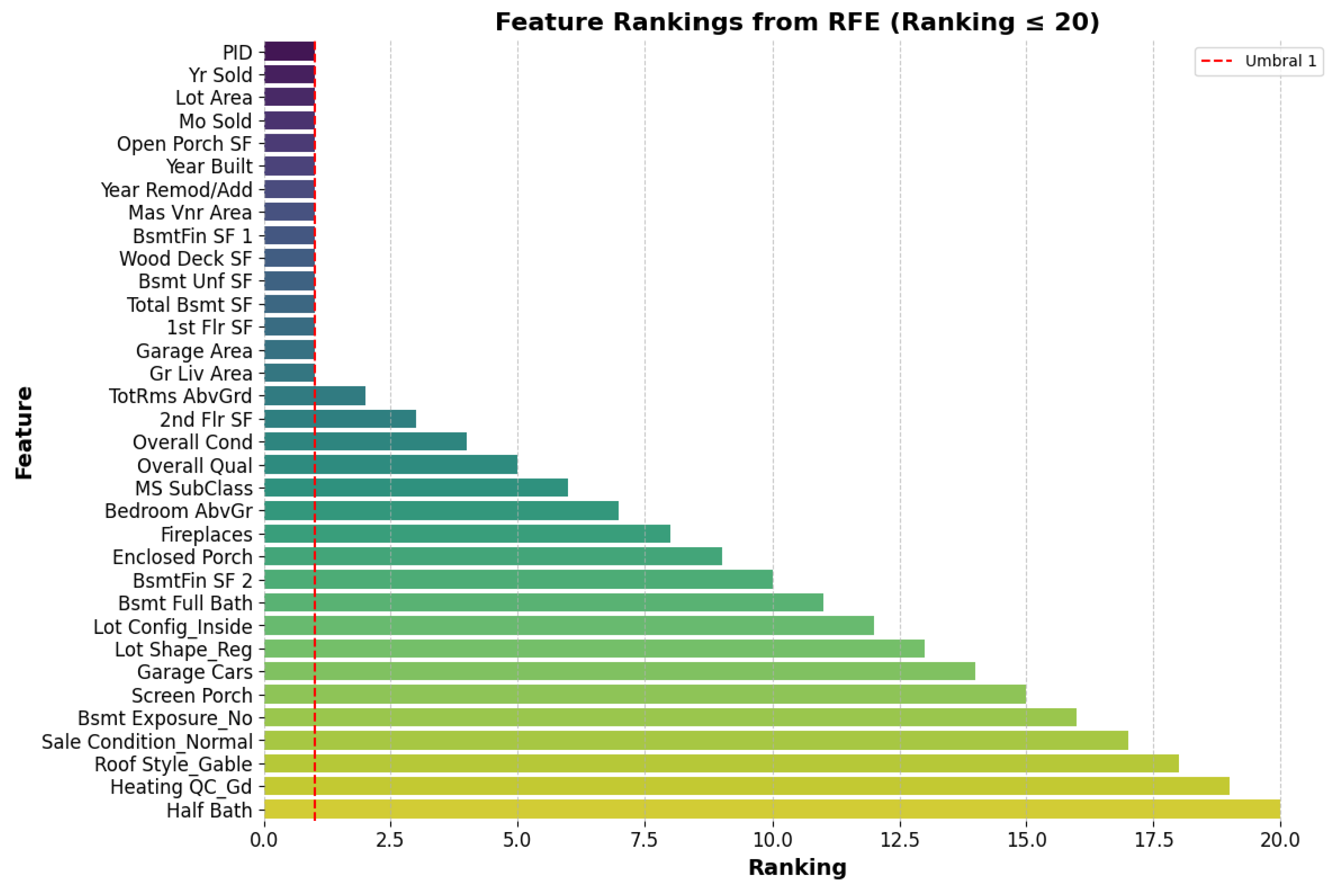
Figure 2.
Application of the RF method for the selection of variables.
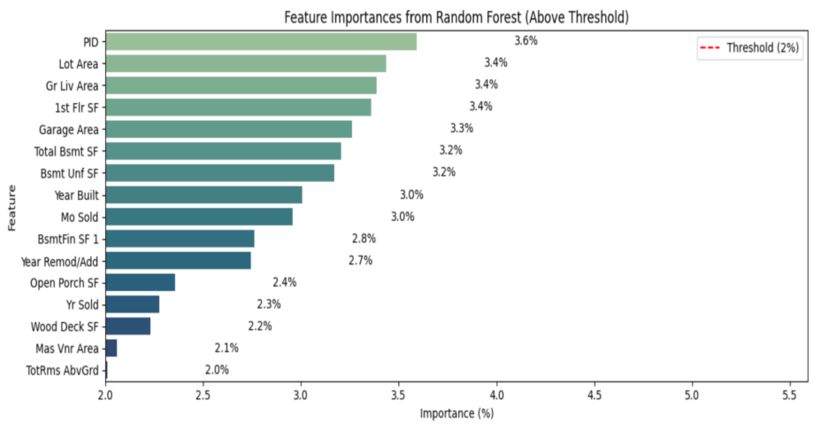
Figure 3.
Application of the Boruta method for the selection of variables.
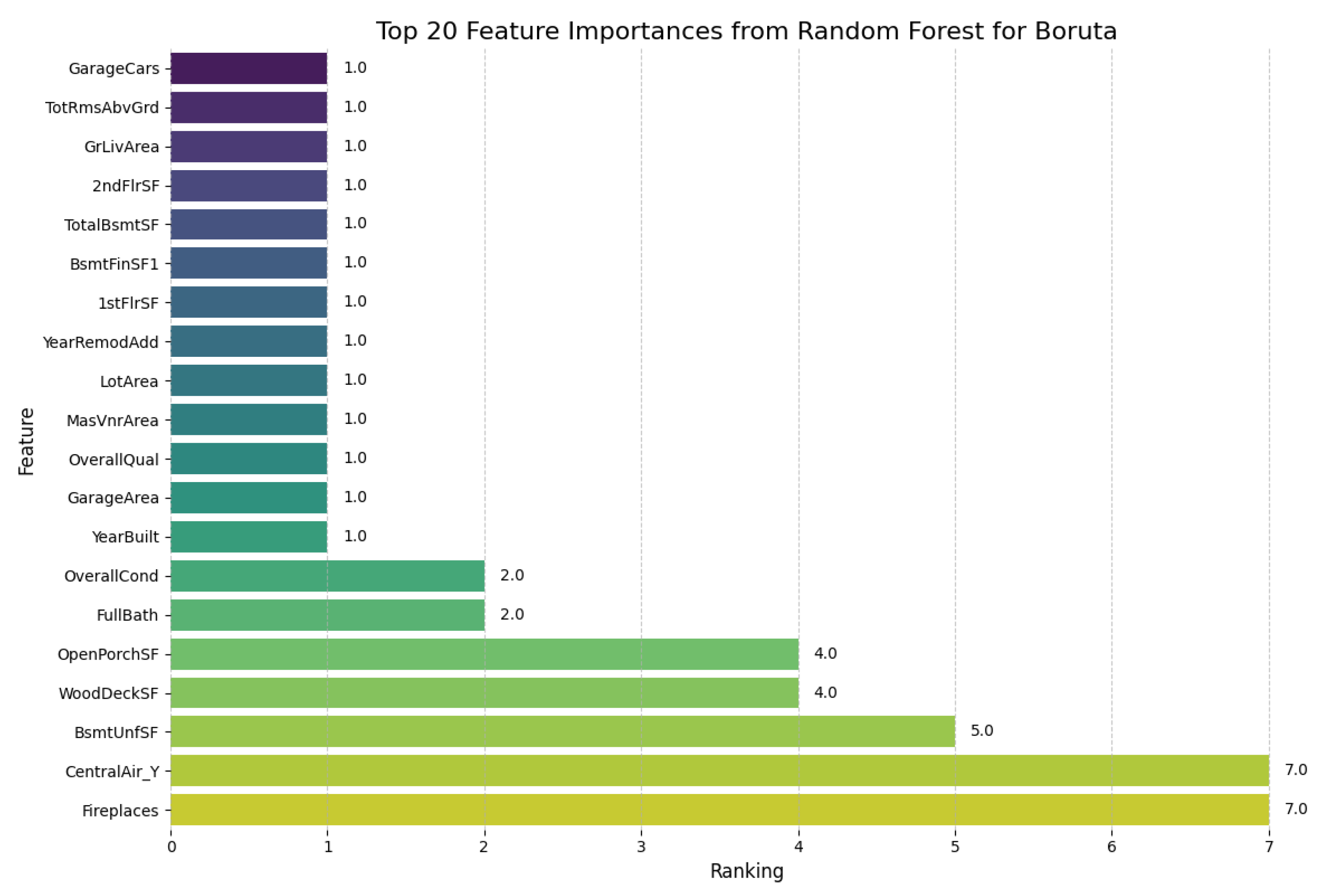

Table 1.
Performance of Machine Learning ensemble models without variable selection and with variable selection through RFE.
Table 1.
Performance of Machine Learning ensemble models without variable selection and with variable selection through RFE.
| Mode | Features | MAE | MSE | RMSE | R2 |
|---|---|---|---|---|---|
| Adaboost | 227 | 23627.919429 | 1.044387e+09 | 32316.982313 | 0.851426 |
| RFE+ Adaboost | 15 | 25392.158815 | 1.173752e+09 | 34260.063181 | 0.833023 |
| Gradient Boosting | 227 | 14536.517194 | 5.642879e+08 | 23754.744694 | 0.919725 |
| RFE + Gradient Boosting | 15 | 17454.651420 | 6.754278e+08 | 25988.994436 | 0.903914 |
| RandomForest | 227 | 15185.544380 | 6.065719e+08 | 24628.680229 | 0.913710 |
| RFE+ RandomForest | 15 | 17535.397304 | 7.454770e+08 | 27303.425108 | 0.893949 |
| ExtraTrees | 227 | 15476.414061 | 6.573662e+08 | 25639.153719 | 0.906484 |
| RFE+ ExtraTrees | 15 | 16762.966974 | 6.782548e+08 | 26043.325620 | 0.903512 |
| Bagging | 227 | 15134.036132 | 6.391276e+08 | 25280.973836 | 0.909078 |
| RFE+ Bagging | 15 | 17429.414198 | 7.574605e+08 | 27522.001198 | 0.892244 |
| Stacking | 227 | 14092.304154 | 5.338036e+08 | 23104.189688 | 0.924062 |
| RFE+ Stacking | 15 | 16505.849309 | 6.473327e+08 | 25442.732864 | 0.907911 |
| Voting | 227 | 15723.876482 | 5.970945e+08 | 24435.517691 | 0.915058 |
| RFE+ Voting | 15 | 17512.356684 | 6.940057e+08 | 26343.988514 | 0.901271 |
Table 2.
Performance of Machine Learning ensemble models without variable selection and with variable selection by RF.
Table 2.
Performance of Machine Learning ensemble models without variable selection and with variable selection by RF.
| Mode | Features | MAE | MSE | RMSE | R2 |
|---|---|---|---|---|---|
| Adaboost | 227 | 23627.919429 | 1.044387e+09 | 32316.982313 | 0.851426 |
| RF+ Adaboost | 16 | 24371.146572 | 1.124288e+09 | 33530.410706 | 0.840060 |
| Gradient Boosting | 227 | 14536.517194 | 5.642879e+08 | 23754.744694 | 0.919725 |
| RF+ Gradient Boosting | 16 | 17308.667825 | 6.725001e+08 | 25932.606461 | 0.904331 |
| RandomForest | 227 | 15185.544380 | 6.065719e+08 | 24628.680229 | 0.913710 |
| RF+ RandomForest | 16 | 17170.938199 | 7.264897e+08 | 26953.472589 | 0.896650 |
| ExtraTrees | 227 | 15476.414061 | 6.573662e+08 | 25639.153719 | 0.906484 |
| RF+ ExtraTrees | 16 | 16776.916428 | 6.684286e+08 | 25853.985352 | 0.904910 |
| Bagging | 227 | 15134.036132 | 6.391276e+08 | 25280.973836 | 0.909078 |
| RF+ Bagging | 16 | 17653.341320 | 7.408339e+08 | 27218.264857 | 0.894610 |
| Stacking | 227 | 14092.304154 | 5.338036e+08 | 23104.189688 | 0.924062 |
| RF+ Stacking | 16 | 16586.994273 | 6.388316e+08 | 25275.118788 | 0.909120 |
| Voting | 227 | 15723.876482 | 5.970945e+08 | 24435.517691 | 0.915058 |
| RF+ Voting | 16 | 17392.159866 | 6.870462e+08 | 26211.565771 | 0.902261 |
Table 3.
Performance of Machine Learning ensemble models without variable selection and with variable selection using Boruta.
Table 3.
Performance of Machine Learning ensemble models without variable selection and with variable selection using Boruta.
| Mode | Features | MAE | MSE | RMSE | R2 |
|---|---|---|---|---|---|
| Adaboost | 227 | 23627.919429 | 1.044387e+09 | 32316.982313 | 0.851426 |
| Boruta+ Adaboost | 16 | 23528.792421 | 1.041813e+09 | 32277.132408 | 0.851793 |
| Gradient Boosting | 227 | 14536.517194 | 5.642879e+08 | 23754.744694 | 0.919725 |
| Boruta+Gradient Boosting | 16 | 16073.472932 | 6.530824e+08 | 25555.476678 | 0.907093 |
| RandomForest | 227 | 15185.544380 | 6.065719e+08 | 24628.680229 | 0.913710 |
| Boruta+ RandomForest | 16 | 15840.843610 | 6.861629e+08 | 26194.711106 | 0.902387 |
| ExtraTrees | 227 | 15476.414061 | 6.573662e+08 | 25639.153719 | 0.906484 |
| Boruta+ ExtraTrees | 16 | 15899.186200 | 7.232086e+08 | 26892.537158 | 0.897117 |
| Bagging | 227 | 15134.036132 | 6.391276e+08 | 25280.973836 | 0.909078 |
| Boruta + Bagging | 16 | 15575.694721 | 6.866662e+08 | 26204.316267 | 0.902315 |
| Stacking | 227 | 14092.304154 | 5.338036e+08 | 23104.189688 | 0.924062 |
| Boruta + Stacking | 16 | 15471.669310 | 6.451969e+08 | 25400.725612 | 0.908215 |
| Voting | 227 | 15723.876482 | 5.970945e+08 | 24435.517691 | 0.915058 |
| Boruta + Voting | 16 | 16228.236364 | 6.583434e+08 | 25658.203542 | 0.906345 |
Disclaimer/Publisher’s Note: The statements, opinions and data contained in all publications are solely those of the individual author(s) and contributor(s) and not of MDPI and/or the editor(s). MDPI and/or the editor(s) disclaim responsibility for any injury to people or property resulting from any ideas, methods, instructions or products referred to in the content. |
© 2025 by the authors. Licensee MDPI, Basel, Switzerland. This article is an open access article distributed under the terms and conditions of the Creative Commons Attribution (CC BY) license (http://creativecommons.org/licenses/by/4.0/).
Copyright: This open access article is published under a Creative Commons CC BY 4.0 license, which permit the free download, distribution, and reuse, provided that the author and preprint are cited in any reuse.


