Submitted:
17 March 2025
Posted:
18 March 2025
Read the latest preprint version here
Abstract
We propose new nonadditive entropy of the apparent horizon $S_K=S_{BH}/(1+\gamma S_{BH}^2)$, where $S_{BH}$ is the Bekenstein--Hawking (BH) entropy and consider the description of new cosmology. When parameter $\gamma$ vanishes ($\gamma\rightarrow 0$) our entropy $S_K$ is converted into BH entropy $S_{BH}$. By using the holographic principle a new model of holographic dark energy is studied. We obtain the generalised Friedmann's equations for Friedmann--Lema\^{i}tre--Robertson--Walker (FLRW) spacetime for the barotropic matter fluid with equation of state $p=w\rho$. From the second modified Friedmann's equation we find a dynamical cosmological constant. The dark energy pressure $p_D$, density energy $\rho_D$ and the deceleration parameter $q$ corresponding to our model are computed. It is shown that at some EoS $w$ and parameter $\gamma$ there are phases of universe acceleration, deceleration and eternal inflation. Our model, with the help of the holographic principle, can describe the universe inflation and late time of the universe acceleration. We show the current deceleration parameter $q_0\approx -0.6$ is realized at some model parameters. The generalised entropy of the apparent horizon with the holographic dark energy model may be of interest for new cosmology.
Keywords:
entropy
; cosmology
; holographic principle
; dark energy
; Friedmann's equations
; universe acceleration
1. Introduction
It is know that black holes can be described by thermodynamics with entropy being proportional to the horizon area [1,2] and temperature is linked with the surface gravity. Thus, gravity is related to ordinary thermodynamics [3,4,5,6]. From the first law of apparent horizon thermodynamics Friedmann’s equations also can be derived [7,8,9,10,11,12,13,14,15,16,17]. Different entropies were studied in [18,19,20,21,22,23,24] which can lead to modified Friedmann’s equations. Other holographic dark energy models were considered in Refs. [25,26,27,28,29,30,31,32,33,34]. Holographic energy densities, depending on the form of entropy, may describe the dark energy which drives the universe to accelerate [35,36]. The nature of dark energy is unknown and can be described by the LCDM model. We propose here new apparent horizon entropy with being the Bekenstein–Hawking (BH) entropy, that lead to the presence of dark energy so that our model is alternative to the LCDM model. The entropy becomes zero when the BH entropy vanishes and is the monotonically increasing function of the BH entropy and is positive. When parameter vanishes we arrive at the BH entropy. It should be noted that the apparent horizon thermodynamics leads to the Friedmann equations, in the framework of Einstein’s gravity, only when the matter is a perfect fluid with equation of state (EoS) with p being the matter pressure and is the density energy of matter [16]. Modifying the BH entropy by apparent horizon entropy we study the general case of EoS for barotropic perfect fluid . It is worth noting that the long-range gravitational interactions are described by generalized entropies. It will be shown that entropy leads to modified Friedmann’s equations that describe the universe inflation. In our approach the cosmological constant is dynamical and it explains the presents of dark energy.
2. New Entropy
Let us consider new entropy
with W being a number of states and each state has a probability with the probability, is a free parameter. The summation in Equation (1) is performed over all possible system microstates. In the case when entropy (1) becomes the Gibbs entropy
If each microstate is populated with equal probability, (), then Equation (2) is converted into the Boltzmann entropy . By virtue of , we find from Equation (1)
The BH entropy is and from Equation (3) one obtains
From Equation (4) we find at the BH entropy . When A and B are two probabilistically independent systems, one has and entropy being the nonadditive entropy because .
3. Thermodynamics of Apparent Horizon
We consider here the FLRW flat universe with the metric
In Equation (5) is a scale factor and represents the line element of 2-dimensional unit sphere. In the FLRW universe the radius of the apparent horizon is given by
where is the Hubble parameter of the universe, and dot over the scale factor being the derivative with respect to the cosmological time t. Inside the space, the total energy is defined as
where, is the energy density of matter fields and the first law of apparent horizon thermodynamics reads
In cosmology the work density W is given by
and p is the matter pressure. The apparent horizon temperature is represented as
Making us of Equations (6), (7), and (9), we obtain from first law of apparent horizon thermodynamics (8) the equation as follows:
With the aid of the energy momentum conservation (the continuity equation)
we find Equation (10) in the form
4. Modified FLRW Equations
Assuming that and making use of Equations (11) and (12), we find
By virtue of our entropy (4) () and BH entropy
and utilizing Equations (13) and (14), one obtains the modified Friedmann equation
Equation (15), as , is converted into the usual Friedmann equation within general relativity for flat universe. Integrating Equation (15) and making use of Equation (12) we find the second modified Friedmann equation
where we have defined parameter . When () Equation (16) becomes the FLRW equation for flat universe in the framework Einstein’s gravity. Introducing the effective (a dynamical) cosmological constant
Equation (16) can be put into the usual form of Friedmann’s equation
The dynamical cosmological constant versus H at some parameters is depicted in Figure 1.
In accordance with Figure 1, increases as the Habble parameter H increases. As the dynamical cosmological constant becomes . At fixed H, when b increases the dynamical cosmological constant also increases. Making use of Equations (17) and (18) we obtain the dark energy density
Let us define the normalized density parameters and , where is the reduced Plank mass. Then from Equations (17), (18) and (19), one finds the equation . By virtue of Equations (17),(18) and (19) we obtain the normalized density of the matter ()
The versus H is plotted in Figure 2.
For the current era , and in accordance with Figure 2, one can obtain the corresponding parameters b and H. Assuming that dark substance obeys ordinary conservation law, and there is no mutual interaction between the cosmos components, we find from the continuity equation the dark energy pressure
With the help of Equations (19) and (21) one obtains the pressure
Making use of Equations (15), (19) and (22) one finds EoS for the dark energy ,
The versus H is plotted in Figure 3.
In accordance with left panel of Figure 3 at and when w increases, EoS parameter for dark energy also increases (at ). According to right panel of Figure 3 at and when b increases, also increases (at ). From Equation (23), it follows that so that the dynamical cosmological constant leads to EoS of dark energy at large Habble parameter H (small apparent horizon radius ). As a result, universe inflation is due to dynamical cosmological constant. When () the dynamical cosmological constant vanishes (). Thus, after Big Bang () we have the de Sitter space, .
According to the second law of apparent horizon thermodynamics we have the requirement and from Equation (4) one obtains or and . As a result, these requirements, for positive Hubble parameter, lead to and . Then from Equation (15) we find that at one has and for the positive energy density we obtain for EoS parameter the requirement .
Now we explore the redshift , where corresponds to a scale factor at the current time. From the continuity Equation (11) and EoS we obtain the density energy of matter
where is the density energy of matter at the present time. With the aid of Equations (16) and (24) one finds equation as follows:
making use of Equations (24) and (25) we obtain the redshift
We plotted the function of Habble parameter versus redshift z in Figure 4 for .
Figure 4 shows that sas redshift z increases the Habble parameter H also increases. According to left panel of Figure 4, when EoS parameter w increases, at fixed z, the H also increases. Right panel of Figure 4 shows that when parameter b increases at fixed z the Habble parameter also increases.
Let us investigate the phases of acceleration and deceleration of the universe. The deceleration parameter is given by
If we have the acceleration phase but when the phase of the universe deceleration takes place. By virtue of Equations (15), (24) and (27) we obtain the deceleration parameter as a function of redshift z
With the help of Equations (25) and (28) one finds the deceleration parameter q in the form
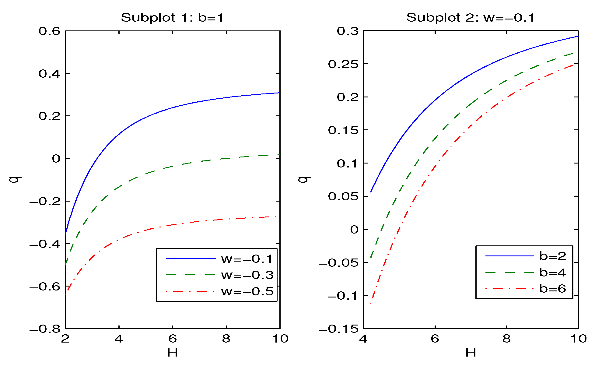
In Figure 5 we depicted the deceleration parameter q versus the Hubble parameter H.
For some values of w and there are two phases: inflation () and deceleration () but at some w and we have only eternal university acceleration (inflation), . In accordance with figure, when redshift z increases the deceleration parameter q also increases. According to left panel of Figure 5, when EoS parameter w increases the deceleration parameter q also increases at fixed . At and there are two phases, acceleration and deceleration but at we have the acceleration phase (the eternal inflation). Accordance to right panel of Figure 5, when parameter b (and ) increases, at fixed w, the deceleration parameter q decreases. At and we have two phases: acceleration and deceleration.
Making use of Equation (29) one obtains the asymptotic
Equation (30) shows that the asymptotic of the deceleration parameter depends only on the entropy parameter (). We obtain from Equation (29 at () that . The approximate real and positive solutions to Equation (29) for H at , , are given in Table 1 for some parameters . When the transition redshifts , we obtained from Equation (26) at .

Table 1.
The approximate solutions to Equation (29) for H at , , .
Table 1.
The approximate solutions to Equation (29) for H at , , .
| 0.2 | 0.3 | 0.4 | 0.5 | 0.6 | 0.7 | 0.8 | 0.9 | 1 | |
| H | 3.777 | 4.180 | 4.492 | 4.749 | 4.971 | 5.166 | 5.341 | 5.501 | 5.648 |
| -3.513 | -3.625 | -3.714 | -3.790 | -3.856 | -3.915 | -1.606 | -1.621 | -1.634 |
Table 2.
The approximate solutions to Equations (3.13) and (3.15) for the current era at , , .
| 0.1 | 0.2 | 0.3 | 0.4 | 0.5 | 0.6 | 0.7 | 0.8 | 0.9 | 1 | |
| H | 3.352 | 3.509 | 3.621 | 3.711 | 3.786 | 3.853 | 3.912 | 3.965 | 4.015 | 4.060 |
| q | -0.618 | -0.646 | -0.664 | -0.676 | -0.686 | -0.694 | -0.701 | -0.707 | -0.712 | -0.717 |
According to Table I shows that when the entropy parameter increases the Hubble parameter H also increases. For a divided point between two pases, universe acceleration and deceleration, the transition reshift is negative and decreases. From Equation (26) we obtain, for the current era when , , approximate solutions for the Habble parameter H and the deceleration parameter q from Equation (29) for different , presented in Table II.
In Table II, negative values of the deceleration parameter q show the acceleration phase of the universe at the current time. The deceleration parameter at the current time is [38]. In accordance with Table II there is entropy parameter which can give that result.
5. Summary
In conclusion, we have proposed new entropy which possesses similar property as the Bekenstein–Hawking entropy SBH; it becomes zero when the apparent horizon radius Rh vanishes. The SK monotonically increases when the apparent horizon radius Rh increases and SK is positive. We have studied the barotropic perfect fluid with flat FLRW universe. By exploring the first law of apparent horizon thermodynamics we obtained the modified Friedmann's equations. We have the addition term in the second Friedmann's equation which is a dynamical cosmological constant. We have showed that holographic dark energy is the source of the universe inflation. It is worth mentioning that Barrow's and Tsallis's entropies also lead to Einsten's equations with the dynamical cosmological constant [37]. We have found that for some parameters our model have phases of universe inflation and deceleration and eternal inflation. The transition redshifts when q = 0, presented in Table I were calculated for some EoS parameter w and for entropy parameter γ. According to Table II, at γ ≈ 0.1 and ω = -2/3 the current deceleration parameter q0 ≈ -0.6 is realised. It was shown that dynamical cosmological constant gives EoS of dark energy ωD = -1 at large Habble parameter H (small apparent horizon radius Rh). So, after Big Bang the de Sitter space takes place (pD + ρD = 0) and universe inflation is due to dynamical cosmological constant. We have showed that when Rh → (H → 0) dynamical cosmological constant vanishes (Λeff → 0). It is worth noting that similar results were discussed in other models [39,40].
Thus, cosmology based on the modified Friedmann equations obtained may be of interest for a description of inflation and late time universe acceleration.
References
- J. D. Bekenstein, Black Holes and Entropy, Phys. Rev. D 7 (1973), 2333-2346.
- S. W. Hawking, Particle creation by black holes, Commun. Math. Phys. 43 (1975), 199-220; Erratum: ibid. 46 (1976), 206.
- T. Jacobson, Thermodynamics of Spacetime: The Einstein Equation of State, Phys. Rev. Lett. 75 (1995), 1260.
- T. Padmanabhan, Gravity and the Thermodynamics of Horizons, Phys. Rept. 406 (2005), 49.
- T. Padmanabhan, Thermodynamical Aspects of Gravity: New insights, Rept. Prog. Phys. 73 (2010), 046901.
- S. A. Hayward, Unified first law of black-hole dynamics and relativistic thermodynamics, Class. Quant. Grav. 15 (1998), 3147-3162.
- M. Akbar and R. G. Cai, Thermodynamic Behavior of Friedmann Equation at Apparent Horizon of FRW Universe, Phys. Rev. D 75 (2007), 084003.
- R. G. Cai and L. M. Cao, Unified First Law and Thermodynamics of Apparent Horizon in FRW Universe, Phys. Rev. D 75 (2007), 064008.
- A. Paranjape, S. Sarkar and T. Padmanabhan, Thermodynamic route to Field equations in Lanczos-Lovelock Gravity, Phys. Rev. D 74 (2006), 104015.
- A. Sheykhi, B. Wang and R. G. Cai, Thermodynamical Properties of Apparent Horizon in Warped DGP Braneworld, Nucl. Phys. B 779, (2007) 1.
- R. G. Cai and N. Ohta, Horizon Thermodynamics and Gravitational Field Equations in Horava-Lifshitz Gravity, Phys. Rev. D 81 (2010), 084061.
- M. Jamil, E. N. Saridakis and M. R. Setare, The generalized second law of thermodynamics in Horava-Lifshitz cosmology, JCAP 1011 (2010), 032.
- Y. Gim, W. Kim and S. H. Yi, The first law of thermodynamics in Lifshitz black holes revisited, JHEP 1407 (2014), 002.
- Z. Y. Fan and H. Lu, Thermodynamical First Laws of Black Holes in Quadratically-Extended Gravities, Phys. Rev. D 91 (2015), 064009.
- R. D’Agostino, Holographic dark energy from nonadditive entropy: cosmological perturbations and observational constraints, Phys. Rev. D 99 (2019), 103524.
- L. M. Sanchez and H. Quevedo, Thermodynamics of the FLRW apparent horizon, Phys. Lett B 839 (2023), 137778.
- S. Wang, Y. Wang and M. Li, Holographic Dark Energy, Phys. Rept. 696 (2017) 1.
- C. Tsallis, Possible generalization of Boltzmann-Gibbs statistics, J. Stat. Phys., 52 (1-2) (1988), 479-487; C. Tsallis, The Nonadditive Entropy Sq and Its Applications in Physics and Elsewhere: Some Remarks, Entropy 13, 1765 (2011).
- A. R´enyi, Proceedings of the Fourth Berkeley Symposium on Mathematics, Statistics and Probability, University of California Press (1960), 547-56.
- A. Sayahian Jahromi et al, Generalized entropy formalism and a new holographic dark energy model, Phys. Lett. B 780 (2018), 21-24.
- J. D. Barrow, The Area of a Rough Black Hole, Phys. Lett. B 808 (2020), 135643.
- G. Kaniadakis, Statistical mechanics in the context of special relativity II, Phys. Rev. E 72 (2005), 036108.
- Marco Masi, A step beyond Tsallis and Rényi entropies. Phys Lett. A 2005, 338, 217–224. [CrossRef]
- V. G. Czinner and H. Iguchi, Rényi entropy and the thermodynamic stability of black holes, Phys. Lett. B 752 (2016), 306-310.
- J. Ren, Analytic critical points of charged Renyi entropies from hyperbolic black holes, JHEP 05 (2021), 080.
- K. Mejrhit and S. E. Ennadifi, Thermodynamics, stability and Hawking–Page transition of black holes from non-extensive statistical mechanics in quantum geometry, Phys. Lett. B 794 (2019), 45-49.
- A. Majhi, Non-extensive Statistical Mechanics and Black Hole Entropy From Quantum Geometry, Phys. Lett. B 775 (2017), 32-36.
- S. Nojiri, S. D. Odintsov and V. Faraoni, From nonextensive statistics and black hole entropy to the holographic dark universe, Phys. Rev. D 105 (2022), 044042.
- S. Nojiri, S. D. Odintsov and T. Paul, Early and late universe holographic cosmology from a new generalized entropy, Phys. Lett. B 831 (2022), 137189.
- S. D. Odintsov and T. Paul, A non-singular generalized entropy and its implications on bounce cosmology, Phys. Dark Univ. 39 (2023), 101159.
- Yassine Sekhmani, et al., Exploring Tsallis thermodynamics for boundary conformal field theories in gauge/gravity duality, Chin. J. Phys. 92 (2024), 894–914.
- Saeed Noori Gashti, Behnam Pourhassan, İzzet Sakallı and Aram Bahroz Brzo, Thermodynamic Topology and Photon Spheres of Dirty Black Holes within Non-Extensive Entropy, Phys. Dark Univ. 47 (2025), 101833.
- J. Sadeghi, B. Pourhassan, and Z. Abbaspour Moghaddam, Interacting Entropy-Corrected Holographic Dark Energy and IR Cut-Off Length, Int. J. Theor. Phys. 53 (2014), 125–135.
- B. Pourhassan, Alexander Bonilla, Mir Faizal, and Everton M. C. Abreu, Holographic Dark Energy from Fluid/Gravity Duality Constraint by Cosmological Observations, Phys. Dark Univ. 20 (2018), 41.
- D. Pavon and W. Zimdahl, Holographic dark energy and cosmic coincidence, Phys. Lett. B 628 (2005) 206.
- R. C. G. Landim, Holographic dark energy from minimal supergravity, Int. J. Mod. Phys. D 25 (2016), 1650050.
- Sofia Di Gennaro, Hao Xu, Yen Chin Ong, How barrow entropy modifies gravity: with comments on Tsallis entropy. Eur Phys. J. C 2022, 82, 1066.
- M. Roos, Introduction to Cosmology (John Wiley and Sons, UK, 2003).
- S. I. Kruglov, Cosmology Due to Thermodynamics of Apparent Horizon. [CrossRef]
- S. I. Kruglov, New entropy, thermodynamics of apparent horizon and cosmology. arXiv:2502.12165.
Figure 1.
The function versus H at . Figure 1 shows that increases as b increases. When the dynamical cosmological constant becomes .
Figure 1.
The function versus H at . Figure 1 shows that increases as b increases. When the dynamical cosmological constant becomes .
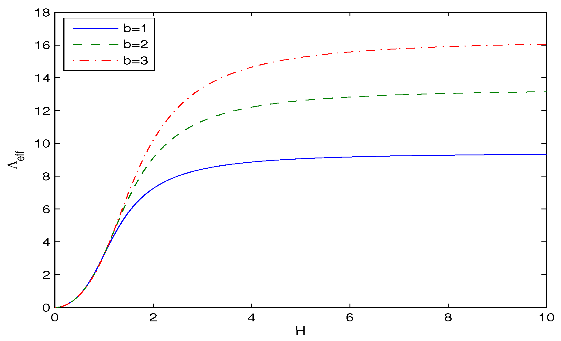
Figure 2.
The function versus H at . According to Figure 2 increases as b decreases at fixed H. When () one has and .
Figure 2.
The function versus H at . According to Figure 2 increases as b decreases at fixed H. When () one has and .
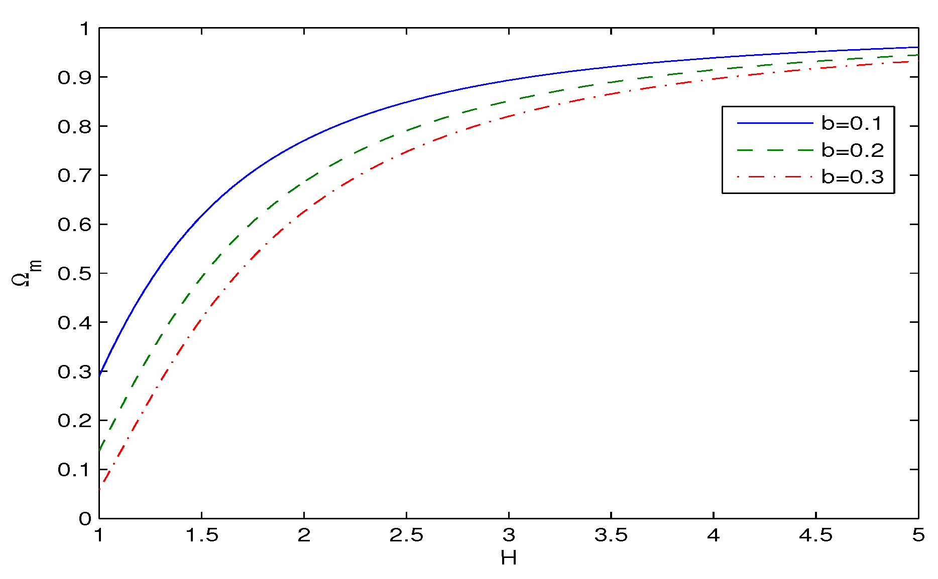
Figure 3.
Left panel: The function versus H at , , . According to Figure 3 when EoS parameter for the matter w increases at fixed H the also increases (at ). At large H EoS parameter for dark energy approaches to . Right panel: In accordance with figure when parameter b increases at fixed H (at ), EoS parameter for dark energy also increases and .
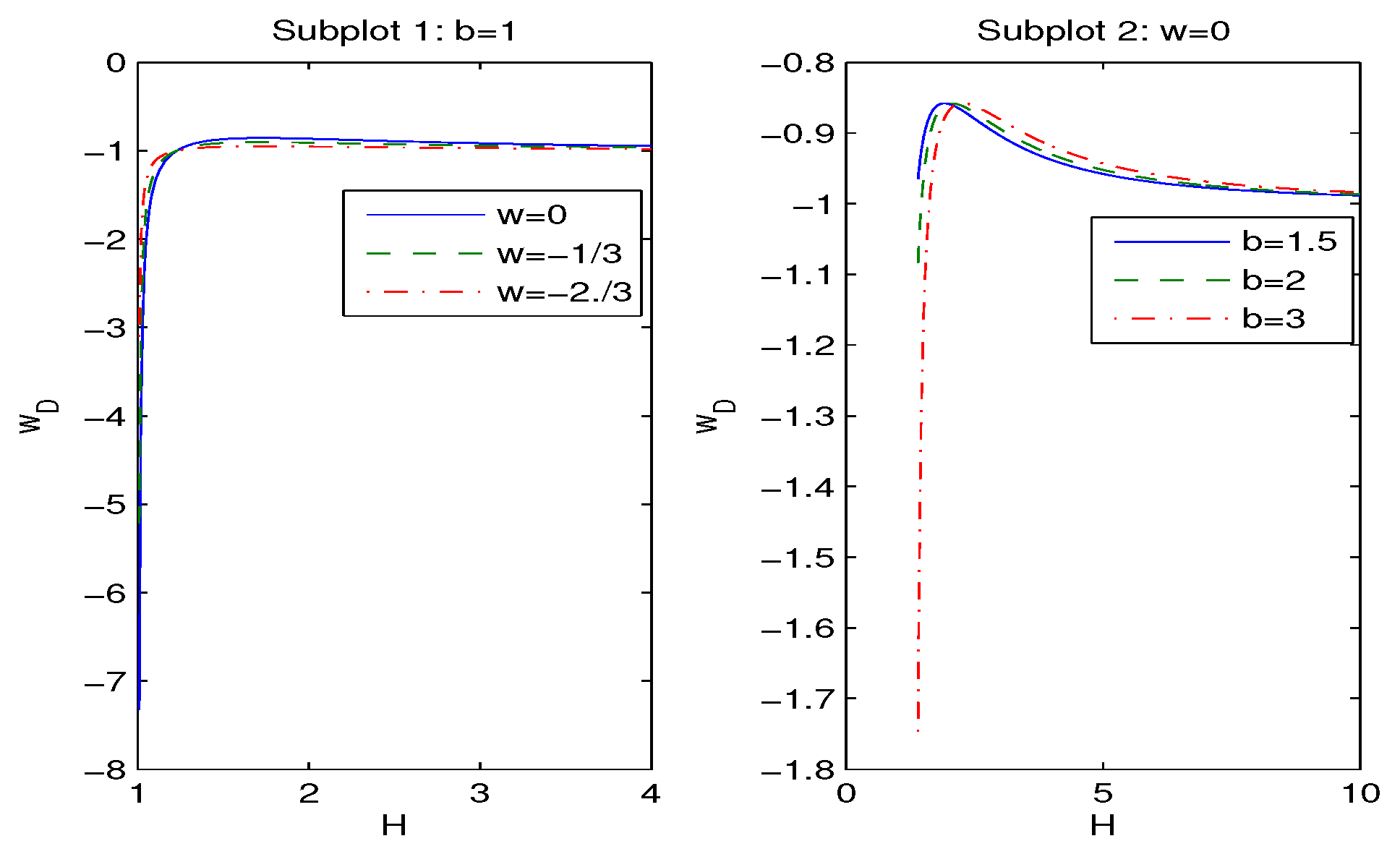
Figure 4.
Left panel: The function H versus z at , , . In accordance with Figure 4 when z increases H also increases. When EoS parameter w increases, at fixed z, the H also increases. Right panel: , , . When parameter b increases at fixed z the Habble parameter also increases.
Figure 4.
Left panel: The function H versus z at , , . In accordance with Figure 4 when z increases H also increases. When EoS parameter w increases, at fixed z, the H also increases. Right panel: , , . When parameter b increases at fixed z the Habble parameter also increases.
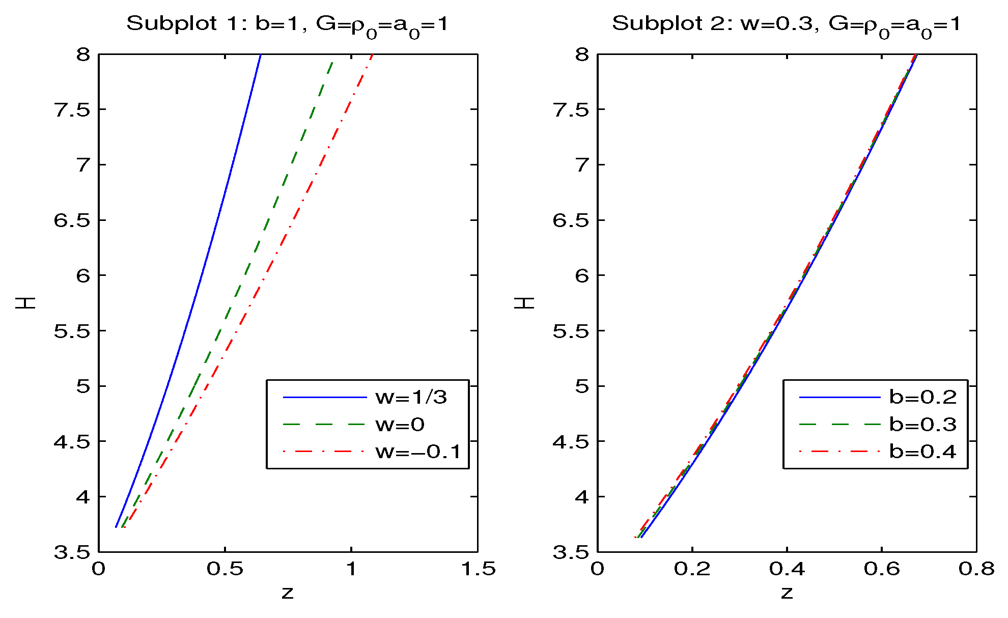
Figure 5.
Figure 5 shows that q increases as H increases. Left panel: The function q versus H at , , -0.5. When EoS parameter w increases at fixed b and H, the deceleration parameter q also increases. At and there are two phases, acceleration and deceleration and at we have only the acceleration phase (the eternal inflation). Right panel: According to figure, when parameter b (and ) increases at fixed w and H the deceleration parameter q decreases. Here, at and we have two phases: acceleration and deceleration.
Disclaimer/Publisher’s Note: The statements, opinions and data contained in all publications are solely those of the individual author(s) and contributor(s) and not of MDPI and/or the editor(s). MDPI and/or the editor(s) disclaim responsibility for any injury to people or property resulting from any ideas, methods, instructions or products referred to in the content. |
© 2025 by the authors. Licensee MDPI, Basel, Switzerland. This article is an open access article distributed under the terms and conditions of the Creative Commons Attribution (CC BY) license (http://creativecommons.org/licenses/by/4.0/).
Copyright: This open access article is published under a Creative Commons CC BY 4.0 license, which permit the free download, distribution, and reuse, provided that the author and preprint are cited in any reuse.


