
Submitted:
17 March 2025
Posted:
18 March 2025
You are already at the latest version
Abstract
In this paper, we use visualization tools to give insight into the performance of six classifiers on multivariate time series data. Five of these classifiers are deep learning models, while the Rocket classifier represents a non-deep learning approach. Our comparison is conducted across twelve datasets from the UEA repository. Additionally, we apply data engineering techniques to each dataset, allowing us to assess classifier performance concerning the available features and channels within the time series. The results of our experiments indicate that the Rocket classifier consistently achieves strong performance across most datasets, while the Transformer model underperforms, likely due to the limited number of instances per class in certain datasets.
Keywords:
multivariate time series classification
; UEA archive
; time series visualization
; deep learning classifiers
1. Introduction
In a multivariate time series classification (MTSC) task, each instance includes multiple measurements observed at each time step. The measurements are referred to as dimensions or channels. In a MTSC task, each observation in a time series has dimensions recorded over time steps, assumed to be aligned in time. For a single instance , we define where each time step . When , we have a univariate time series dataset. The MTSC archive is included in the UEA repository, which also contains univariate time series datasets.
In our work, we considered six classification algorithms, and fifteen multivariate time series datasets sourced from the UEA repository. In particular, we have included a hybrid algorithm (CNN-1D-LSTM) and a novel algorithm: Transformers. We visualized the pattern of channels and features for each dataset to gain insights into how they influence classifier accuracy. Additionally, we performed feature selection on the training data, and we assessed the similarity between training and testing data to understand its impact on classification performance. In each dataset, the stationarity of the time series is evaluated, since might have influence in the classifier performance.
This paper is organized as follows: Section 2 reviews related work. Section 3 details the methodology of our experiments, including brief descriptions of the six classification algorithms and the datasets used. Section 4 presents and discusses the results obtained in our experiments for each of the fifteen datasets, as well as general observations. Finally, Section 6 provides our conclusions and suggests directions for future work.
2. Related Work
Bagnal et al. [1,2] described 30 datasets for multivariate time series classification (MTSC), where each instance includes multiple measurements observed at each time step. They presented classification results in an overall summary rather than individually for each dataset. These datasets form the UEA repository. Fawaz et al. [3] reviewed MTSC using deep learning algorithms, providing global classifier accuracy results across both univariate and multivariate datasets. However, their repository differs from ours. They employed two visualization tools: Class Activation Maps (CAMs) to provide interpretable feedback that highlights classifier decision rationale and Multi-Dimensional Scaling (MDS) to illustrate the spatial distribution of input time series across different classes. These visualization techniques were applied only to univariate time series data.
Baldan and Benitez [4] proposed an MTSC method based on an alternative representation of time series, using 41 descriptive time series features. They utilized the 30 MTSC datasets available in the UEA repository. Pasos Ruiz et al. [5] conducted an extensive review and experimental evaluation of 16 algorithms on 26 multivariate time series datasets. In our work, we have included three of these algorithms and excluded ensemble methods such as CIF and HIVE-COTE, while considering 15 datasets.
Pasos Ruiz and Bagnall [6] explored several strategies for selecting optimal channels in MTSC when using the HIVE-COTE v2.0 classifier. Finally, Ilbert et al. [7] applied data augmentation techniques to MTSC datasets, given that most of the UEA’s datasets contain a limited number of instances, although their findings showed minimal improvement in classifier accuracy.
3. Methodology
3.1. Classification Algorithms
In this paper, we consider six classifiers: the Random Convolutional Kernel Transform (ROCKET), the Residual Network (ResNet), the Inception Time algorithm, a one-dimensional CNN, the CNN1D-LSTM model, and the Transformer algorithm. We excluded the HIVE-COTEv2 algorithm, a heterogeneous meta-ensemble for MTSC, due to its limited scalability with respect to dimensionality and time series length [5]. For the same reason, other ensemble methods were also not considered. In the following sub-sections, we briefly explain each of the algorithms used.
3.1.1. The Random Convolutional Kernel Transform (ROCKET)
The Random Convolutional Kernel Transform (ROCKET), introduced by Dempster et al. [8], utilizes numerous random convolution kernels combined with a linear classifier, such as ridge regression or logistic regression. Each kernel is applied to every instance, producing feature maps from which the maximum value and a novel feature, the proportion of positive values (ppv), are extracted. For each of the 10,000 generated kernels, parameters are drawn from specific distributions: The length is selected such that, ; the value of each weight, , in the kernel is selected such that, ; dilation is sampled from an exponential scale up to the input length, and the binary decision to pad the series is chosen with equal probability. If padding is applied, the series is zero-padded at both ends, allowing the kernel’s midpoint to be applied to each point in the input series.
The convolution operation between an instance and a kernel can be interpreted as a dot product of two vectors, resulting in a feature map used to calculate the maximum value and ppv features. The ppv captures the proportion of the series correlated to the kernel, which has been shown to enhance classification accuracy. After all convolutions, each series is transformed into an instance with 20,000 attributes, which is then used to train the ridge regression classifier. An extension to the ROCKET approach to enable use on multivariate datasets has recently been added to the Python’s sktime library [9]. For application on multivariate datasets, kernels are assigned to random dimensions. Weights are then generated for each channel. Here, convolution is interpreted as a matrix dot product as the kernel convolves horizontally across the series, and the maximum and ppv values are calculated across all dimensions for each kernel, producing a 20,000-attribute instance.
In most cases, ridge regression is preferred due to its efficiency in cross-validating the regularization hyperparameter. However, for very large datasets where the number of instances significantly exceeds the number of features, logistic regression with stochastic gradient descent offers greater scalability. ROCKET effectively zooms out the time series data in a manner analogous to how Support Vector Machines (SVM) operate on data points.
3.1.2. Residual network (ResNet)
ResNet was first applied to time series classification in [10]. It consists of three consecutive blocks, each containing three convolutional layers connected by residual ’shortcut’ connections, which add each block’s input to its output. These residual connections facilitate the direct flow of gradients through the network, helping to mitigate the vanishing gradient problem. Following the residual blocks, global average pooling and softmax layers are used to generate features and make predictions. We retain all hyperparameter and optimizer settings from Fawaz et al.’s evaluation [3]. The implementation in sktime [9] interfaces with the original implementation provided by their study.
3.1.3. InceptionTime
InceptionTime achieves high accuracy by building on ResNet to incorporate Inception modules [10] and by assembling over five multiple random-initial-weight instantiations of the network to improve stability [11]. Each network in the ensemble consists of two blocks, each containing three Inception modules, as opposed to ResNet’s structure of three blocks with three traditional convolutional layers. These blocks retain residual connections and are followed by global average pooling and softmax layers, as in ResNet.
An Inception module takes an input multivariate series of length and dimensionality . It first applies a bottleneck layer with filter length and stride of 1 to reduce the dimensionality to , maintaining the original series length . This dimensionality reduction significantly decreases the number of parameters. Convolutions of varying lengths are then applied to the bottleneck layer’s output to detect patterns of different sizes. The outputs of these convolutions are combined with an additional source of diversity, a Max Pooling followed by bottleneck (with the same value of d’) applied to the original time series, and all stacked to form the dimensions of the output multivariate time series to be fed into the next layer. Once more, we maintain all hyperparameter settings and optimizer settings from the source article [12], and the implementation in sktime [9] is an interfacing of the implementation provided by that study.
3.1.4. One Dimensional Convolutional Neural Network (CNN-1D)
There are numerous CNN architectures, such as LeNet, AlexNet, and GoogleNet [13], used to classify multivariate time series. In this work, we employed a sequential model for CNN, specifically a 1D CNN [14,15], which is well-suited for analyzing sequential data like time series and spectral data. Each time series is represented by the input shape parameter of the Conv1D layer with a given number of feature maps (filters) and kernel size. The feature maps determine the number of times the input is processed or interpreted, whereas the kernel size specifies the number of input time steps considered as the input sequence is read or processed onto the feature maps.
In our experiments, we varied the number of feature maps between 32 and 256 and used kernel sizes of either 2 or 3. Following the Conv1D layer, we applied a MaxPooling1D layer with a pool size of 3, repeating this sequence of layers three times. Afterward, a Flatten layer was added, followed by three dense layers with 64 neurons each. The output layer matched the number of dataset classes and used the softmax activation function. Given that most datasets have a limited number of features, we did not include a dropout layer.
The architecture of the 1D CNN model used for the SCP1 dataset is shown in Figure 1. We trained the model for 30 epochs with a batch size of 256, optimizing the categorical cross-entropy loss function using the ADAM optimizer, a variant of stochastic gradient descent.
3.1.5. CNN-1D - LSTM
In the MLP model, the pre-layer and post-layer are fully connected, with no connections among neurons within the same layer. In contrast, the Recurrent Neural Network (RNN) introduces a weighted sum of the previous inputs into the hidden layer’s calculation, allowing it to consider both the output from the previous layer and all prior outputs [16]. This feedback mechanism in the hidden layer helps the network learn context-related information, making RNNs effective for processing sequential data, such as time series and spectral data.
However, RNNs are limited by short-term memory, struggling to retain information over long sequences. Long Short-Term Memory (LSTM) networks, a type of RNN, address this by managing long-term dependencies between inputs and outputs [17,18]. LSTM networks use internal mechanisms called gates to regulate the flow of information, enabling the network to learn which data in a sequence is important to retain or discard. This capability allows LSTMs to pass relevant information along the sequence, helping improve predictions over long input chains.
3.1.6. Transformers
Vaswani et al. [19] introduced the concept of attention-based networks, originally designed for natural language processing (NLP), where sequences of words are ordered by grammar and syntax. In an attention-based network, known as the Transformer, an input sequence (e.g., text in English) is processed to generate an output sequence (e.g., text in Spanish). In time series analysis, where data is ordered chronologically in time steps, the Transformer generates a forecast along the time axis from a sequence of training observations. Transformers are effective in capturing long-range dependencies and interactions, making them well-suited for time series modeling. In many applications, Transformers have demonstrated superior performance compared to RNN and LSTM models [20,21,22].
A key feature of the Transformer is its attention heads, which enable it to learn relationships between each time step and every other time step in the input sequence. Transformer dynamically updates attention weights to emphasize relevant time steps and downgrade less relevant ones, with a score matrix expressing the association between each time step and the others.
The Transformer architecture consists of a stack of Encoder and Decoder layers, each with corresponding Embedding layers for their respective inputs. The final Output layer generates the model’s predictions. Each attention block within the architecture includes components such as Self-Attention, Layer Normalization, and a Feed-Forward layer. The input dimensions of each block are equal to its output dimensions.
3.2. Datasets
In this paper, we use only 15 of the 30 MTSC datasets available in the UEA repository, discarding others for the following reasons. Four datasets—Insect Wingbeats, Spoken Arabic Digits, Character Trajectories, and Japanese Vowels—contain unequal-length time series. These were excluded to avoid preprocessing steps that could impact classifier comparisons. Additionally, four datasets—AtrialFibrillation, BasicMotions, ERing, and StandWalkJump—have less than 50 instances in their training sets, which can be problematic for deep learning algorithms that require a larger number of instances to achieve reliable prediction performance. Despite this, we have included the BasicMotions dataset in our experimental study.
There are also four datasets—Libras, LSST, PendDigits, and RacketSports—containing time series of very short length (less than 50 points), which may limit the predictive power of machine learning algorithms. In our study, we have considered two of these datasets: Libras and RacketSports. Conversely, two datasets, EigenWorms and MotorImagery, feature very long time series (over 2000 points), which can overwhelm the algorithms and reduce prediction accuracy. Binning can be used to reduce the dimensionality but to carry out a fair comparison, we prefer to exclude both datasets. The Phoneme dataset was also excluded due to its limited training set for a large number of classes (39), which could impair model performance.
Lastly, the Cricket, Handwriting, and UWaveGesture datasets were excluded due to their small training sets relative to their testing sets, resulting in poor performance for deep learning models. For these datasets, the product of training size and dimensionality is low, leading to underperformance in deep learning algorithms.
In the following sections, we provide a brief overview of the datasets included in our experiments, listed in descending order based on the average accuracy achieved by the classifiers considered in our experiments.
3.2.1. Epilepsy (EPI)
The data presented in [23] was generated using a 3D accelerometer worn on the dominant wrist, with healthy participants simulating specific class activities. An accelerometer measures changes in speed and typically reports data across three movement axes (x, y, z). Data was collected from six participants using a tri-axial accelerometer as they performed four different activities, each with varying durations. The four tasks, each of different length, are: i) Walking includes different paces and gestures: walking slowing while gesturing, walking slowly, walking normal and walking fast, each of 30 seconds long; ii) Running includes running a 40 meters long corridor; iii) Sawing with a saw and for 30 seconds; and iv) Seizure mimicking whilst seated, with 5-6 sec before and 30 sec after the mimicked seizure. The seizure was 30 sec long. Each participant performs each activity 10 times at least. As a standard practice for the dataset, data was truncated to match the length of the shortest retained series. One case (ID002 Running 16) was removed due to incomplete data collection. After cleaning, the dataset consists of 275 cases, with 137 instances in the training set, approximately equally distributed among the four classes, and 138 instances in the test set.
3.2.2. NATOPS
This dataset, adapted from the 2016 Advanced Analytics and Learning on Temporal Data challenge [24], contains 24-dimensional data recorded via Xbox Kinect as participants performed one of six gestures. Sensors attached to each hand, elbow, wrist, and thumb captured 3D positional data throughout each gesture. The training set consists of 180 instances, equally distributed across the six classes, and the test set also contains 180 instances.
3.2.3. Articulacy Word Recognition (AWR)
An Electromagnetic Articulograph (EMA) is a device used to measure tongue and lip movements during speech by tracking small sensors attached to the articulators (e.g., tongue, lips). Subjects are seated within a calibrated magnetic field, allowing for precise measurement of sensor position changes. The EMA AG500 achieves a spatial accuracy of 0.5 mm.
Data was collected from multiple native English speakers as they produced 25 words [25]. Nine sensors, each recording x, y, and z positions at a 200 Hz sampling rate, were used in data collection. The sensors were placed on the forehead, jaw, lips, and along the tongue from tip to back in the midline. Three head sensors (Head Center, Head Right, and Head Left) were mounted on a pair of glasses to account for head-independent movement of other sensors. Tongue sensors were labeled T1 through T4, from tip to back. Out of 27 available dimensions, this dataset includes only nine.
3.2.4. SelfRegulationSCP1 (SCP1)
In this dataset, healthy participants were asked to visualize moving a cursor either up or down on a screen. The direction of movement was determined by their Slow Cortical Potential (SCP), measured via EEG and visually fed back to the participant [26]. EEG data was recorded from six positions on the head. The objective is to classify each instance as positive (downward) or negative (upward) movement based on EEG readings.
During each trial, the task was visually indicated with a highlighted goal at either the top (positive) or bottom (negative) of the screen, starting from 0.5 seconds until the end of the trial. Visual feedback was provided between 2 and 5.5 seconds. Only this 3.5-second interval is used for training and testing. With a sampling rate of 256 Hz and a recording length of 3.5 seconds, each trial includes 896 samples per channel.
The training data consists of 268 trials, with 135 trials for one class and 133 for the other, recorded over two separate days and randomly mixed. The test set includes 293 trials.
3.2.5. PEMS-SF
This is a UCI dataset provided by the California Department of Transportation, as reported in [27]. It contains 15 months of daily data from the California Department of Transportation’s PEMS website, covering the period from January 1, 2008, to March 30, 2009 (455 days in total). The data represents the occupancy rate (between 0 and 1) of various freeway lanes in the San Francisco Bay Area, sampled every 10 minutes.
Each day in the dataset is represented as a single time series with 963 dimensions, corresponding to the sensors that consistently operated throughout the period, and a length of 144 time steps (6 samples per hour over 24 hours). Public holidays were excluded from the dataset, along with two days containing anomalies—March 8, 2009, and March 9, 2008—when all sensors were muted between 2:00 and 3:00 AM. This results in a dataset of 440 time series, each representing a day of data.
The task is to classify each time series by its corresponding day of the week, from Monday (label 1) to Sunday (label 7).
3.2.6. Heartbeat (HB)
This dataset is derived from the PhysioNet/CinC Challenge 2016 [28] and consists of heart sound recordings sourced from various contributors worldwide. Recordings were made in both clinical and nonclinical environments, from both healthy subjects and patients with confirmed cardiac conditions. Heart sounds were collected from different locations on the body, typically including the aortic, pulmonic, tricuspid, and mitral areas, though recordings could come from any of nine possible locations.
The recordings are categorized into two classes: normal (from healthy subjects) and abnormal (from patients with confirmed cardiac diagnoses). Both healthy subjects and patients include adults and children. Each recording was truncated to a standard length of 5 seconds. Spectrograms of each instance were then generated with a window size of 0.061 seconds and a 70% overlap. In this multivariate dataset, each dimension represents a frequency band from the spectrogram. The dataset includes 113 patients in the normal class and 296 in the abnormal class.
3.2.7. Face Detection (FD)
This dataset is derived from the training set of a Kaggle competition [29] and consists of Magnetoencephalography (MEG) recordings with class labels (Face/Scramble) from 10 subjects (subject01 to subject10). Test data is available for an additional six subjects (subject11 to subject16). For each subject, approximately 580-590 trials are included. Each trial contains 1.5 seconds of MEG recordings, beginning 0.5 seconds before the stimulus onset, along with a corresponding class label: Face (class 1) or Scramble (class 0).
The MEG data was down-sampled to 250 Hz and high-pass filtered at 1 Hz. The original dataset includes 306 time series channels, each containing 375 time steps. For this study, we used a reduced set of 144 channels and 62 time steps, as provided on the competition website. Trials for each subject are organized into a 3D data matrix with dimensions (trial x channel x time), resulting in matrices of size 580 x 144 x 62. The training set comprises 5,890 instances, evenly split between the two classes.
3.2.8. Duck Duck Geese (DDG)
This dataset was derived from audio recordings available on the Xeno Canto website [30]. Each recording was selected from either the A or B quality category. Due to varying sample rates among the recordings, all audio files were downsampled to 44,100 Hz. Each recording was then center truncated to a length of 5 seconds (matching the length of the shortest recording) before being transformed into a spectrogram with a window size of 0.061 seconds and an overlap of 70%. The dataset includes the following classes: Black-bellied Whistling Duck (20 instances); Canadian Goose (20 instances); Greylag Goose (20 instances); Pink Footed Goose (20 instances); and White-faced Whistling Duck (20 instances).
3.2.9. Finger Movements (FM)
This dataset, described in [31], consists of 500 ms intervals of Electroencephalogram (EEG) recordings, starting 130 ms before a key press. A single participant, seated in a normal position at a keyboard, was instructed to type characters using only the index and pinky fingers. The dataset has 28 dimensions, each with 50 attributes, and includes two target classes: left and right. The training set contains 316 instances, with 159 labeled as the first class and 157 as the second. The test set includes 100 instances.
3.2.10. SelfRegulationSCP2 (SCP2)
An artificially respirated ALS patient was instructed to move a cursor either up or down on a screen. The direction of movement was controlled via Slow Cortical Potential (SCP), measured using EEG, and provided to the participant both visually and audibly [26]. EEG data was recorded from seven positions on the head. The objective is to classify each instance as positive (downward) or negative (upward) movement based on EEG readings.
During each trial, the task was indicated by a highlighted goal at the top (indicating negativity) or bottom (indicating positivity) of the screen from 0.5 to 7.5 seconds. Additionally, the task (“up” or “down”) was vocalized at 0.5 seconds. Visual feedback was provided from 2 to 6.5 seconds. Only the 4.5-second interval from 2 to 6.5 seconds is available for training and testing.
With a sampling rate of 256 Hz over 4.5 seconds, each trial consists of 1152 samples per channel. The training data contains 200 trials (100 of each class), recorded on the same day and permuted randomly. Each time series has a length of 1152 across 7 dimensions. The test set includes 180 trials.
3.2.11. Hand Movement Direction (HMD)
This dataset includes recordings from two right-handed subjects moving a joystick with their hand and wrist in one of four possible directions (right, up, down, or left) after hearing a prompt. The task is to classify the direction of movement based on the resulting MEG data. Each recording captures an interval beginning 0.4 seconds before the movement and ending 0.6 seconds afterward, across 10 MEG channels. The data is sampled at 400 Hz (see [29] for more details). The training set consists of 160 instances, with 40 instances per direction. The test set includes 74 instances.
3.2.12. Ethanol Concentration (EC)
The Ethanol Concentration dataset contains raw spectra of water-and-ethanol solutions in 44 unique whisky bottles [32]. The ethanol concentrations are set at 35%, 38%, 40%, and 45%, and the classification task is to determine the alcohol concentration of a sample in an arbitrary bottle. Each instance in the dataset includes three repeated readings from the same bottle and batch of solution. Three batches of each concentration were prepared, with each bottle-batch combination measured three times. For each reading, the bottle was picked up, placed between the light source and spectroscope, and the spectra recorded. Spectra were captured across the full wavelength range of the Stellar-Net BLACKComet-SR spectrometer (226 nm to 1101.5 nm, with a sampling interval of 0.5 nm) over a one-second integration time.To simulate potential real-world conditions for large-scale screening, no special precautions were taken to obtain pristine readings or to replicate the exact light path through the bottle for each repeat reading, aside from avoiding labeled, embossed, or seamed areas on the bottle.
3.2.13. Basic Motions (BM)
This dataset was collected by students at UEA. Data was generated by participants performing four activities while wearing a smart watch. The watch collected 3D accelerometer and gyroscope data. The dataset consists of four classes: walking, resting, running and playing badminton. Participants were required to record each motion a total of five times. The sample rate of both sensors was 10Hz and activity was recorded for 10 seconds. The training set consists of 40 instances. Each time series has a length of 100 across 6 channels. The test set includes 40 instances.
3.2.14. Racket Sports (RS)
This dataset was collected by students at UEA. The dataset consists of data recorded while participants were playing one or two strokes during the time that they were playing badminton or squash. The data was captured through a smart watch (Sony smart watch 3) worn on the participant’s dominant hand. The watch relayed the x, y, z values for both the gyroscope and the accelerometer. Th0e task is to classify which sport, and which stroke the players are making. The data was collected at a rate of 10Hz, over 3 seconds while the participant was playing either a forehand/backhand in squash or a clear/smash in badminton. The training set consists of 151 instances. Each time series has a length of 30 across 6 channels. The test set includes 152 instances.
3.2.15. Libras (LIB)
LIBRAS (“Lingua Brasileira de Sianis”) is the official Brazilian sign, This dataset contains 15 classes each of them with 24 instances, Each class represents a hand movement type in LIBRAS. The hand movement is represented by a bi-dimensional curve performed by the hand in a period of time. This hand movement is extracted from a video. From each video 45 frames were selected uniformly to extract the hand movement (see [33] for more details). The whole dataset was equally spitted into training sets. Thus, both have 180 instances. Each time series has a length of 3 across 6 channels.
Our research workflow is as follows:
First, we load the dataset from the UEA repository.
Second, we plot the mean values by channel in each group.
Third, we compute the distance between the groups through the Euclidean distance between the mean vector of each channel. If this distance is small the dataset is hard to classify.
Fourth, we carry out feature selection using either the F-test criterion for normalized data or the Mutual Information criterion for unnormalized data.
Fifth, we plotted the mean of the time series in each group of both the training and testing set and compute the Euclidean distance between the mean values of the training and testing set. If this distance is small then the distribution of training and testing is quite similar. Otherwise, the distributions are different, and the classifier algorithm will not perform well.
Sixth, stationarity tests and their p-values are computed.
Finally, the classifier algorithm is applied and evaluated.
In Table 1 a summary of the datasets is presented in descending order according to the accuracy obtained
4. Experimental Results
4.1. Overall Results
Table 2 provides a summary of our study’s results, presenting the mean and standard deviation of test set accuracy across 10 runs for each dataset and algorithm combination. The ROCKET algorithm was executed with 20,000 kernels, ResNet was configured with 300 epochs and a batch size of 16, while Inception Time was run with 200 epochs and a batch size of 64. For the deep learning algorithms—CNN1D, CNN1D-LSTM, and Transformers—we used 300 epochs with a batch size of 32. All experiments were implemented in Python 3.10.9 using scikit-learn, Keras, and TensorFlow 2.0. The best results are highlighted in bold; for some datasets, two algorithms are bolded due to statistically similar performance. To compare all six algorithms, we employed the non-parametric Wilcoxon test in a pairwise setup.
4.2. Individual Results
In this section, we present graphics and metrics to illustrate the behavior of features and channels in each dataset. Furthermore, we report results on feature selection for each training dataset: for normalized data, we use the F-test, and for unnormalized data, we apply the Mutual Information criterion.
4.2.1. Epilepsy (EPI)
Some features appear relevant for classification, as indicated in Figure 2, which presents the mean time series for each class. Additionally, 19.41% of features in the training data exceed the F-test p-value threshold of 0.10. Figure 3 displays the mean time series for each channel across groups, highlighting that only the first class poses classification challenges. Figure 4 provides boxplots for each channel in both the training and test datasets, showing similar distributional behavior across channels. The Euclidean distance between the mean vectors of the training and test data is 6.9673. Figure 5 illustrates the mean time series for each group in both datasets, revealing comparable time series patterns.
These visualizations collectively suggest strong classifier performance, indicating that the features’ behavior contributes more significantly to the classification task than channel-specific patterns.
4.2.2. NATOPS
In this dataset, all 51 features are deemed relevant according to the F-test (100%). Figure 6 displays the mean values of all the time series for each of the six groups. The Euclidean distance between the mean vectors for groups ranges from a minimum of 0.17 to a maximum of 1.78, suggesting that training the classifier is unlikely to pose significant difficulty. However, there is considerable overlap among the mean time series for each channel across groups. Additionally, the feature distributions in the training and testing datasets are highly similar, with a Euclidean distance of only 0.31 between their mean vectors. Consequently, in the NATOPS dataset, classifier accuracy appears to rely more heavily on feature behavior than on channel-specific patterns.
4.2.3. Articulacy Word Recognition (AWR)
Most channels appear relevant for the classification task, as suggested by Figure 7. While the F-test did not identify any features as relevant, this may be attributed to the large number of classes (25), which can affect the F-test’s sensitivity. Similarly, the Mutual Information criterion did not identify any relevant features. The Euclidean distance between the mean vectors across groups ranges from 0.022 to 0.094, with substantial overlap observed among the mean time series across groups. Additionally, the feature distributions in the training and testing datasets are highly similar, with a Euclidean distance of only 0.63 between their mean vectors. These findings suggest that channel behavior plays a more significant role than feature characteristics in this classification task.
However, due to the dataset’s high class count (25) and limited instances per class (11), Transformers performance is impacted. Excluding Transformers, this dataset yielded the highest classifier performance. Although we applied dimension selection using the sktime library, this did not improve Transformer performance.
4.2.4. SelfRegulationSCP1 (SCP1)
Figure 8 shows a clear separation between the mean values per channel throughout the time series, except at the beginning. According to the F-test, the majority of features (68.41%) are relevant for the classification task. However, Figure 9 reveals minimal separation between the mean values of all time series across groups, with a Euclidean distance of only 0.29 between group mean vectors. This suggests that channel information may play a more critical role than feature characteristics in classification.
The Euclidean distance between the mean vectors of the training and test datasets is notably large, at 1022.68, indicating a significant difference between these sets. The unnormalized time series values range between -10 and 30.
4.2.5. PEMS-SF
According to the F-test, most features are irrelevant for classification, with only 0.69% showing relevance, while the Mutual Information criterion identifies 9.03% of relevant features. This finding is supported by Figure 10 and the minimal Euclidean distance between group mean vectors, ranging from 0.022 to 0.094. Conversely, Figure 11 indicates some separation in mean values for certain channels across at least four groups, while the remaining three groups exhibit significant overlap. Figure 11 should show seven colors one for each group, but some of them are hard to be noticed.
The distribution of features in the training and testing datasets is relatively similar, as indicated by a Euclidean distance of 1.45 between their mean vectors. These observations suggest that channel characteristics are more critical than features in determining classifier accuracy.
4.2.6. Heartbeat (HB)
This dataset exhibits class imbalance in the training set, with 147 instances in one class and 57 in the other, which impacts classifier performance. The F-test criterion identifies only 2.22% of features as relevant for classification, while the Mutual Information criterion suggests that 15.55% of features are significant. The mean values across groups are quite similar, as indicated by the low Euclidean distance of 0.01867 between group mean vectors.
Figure 12 highlights significant overlap in the mean values of channels across the two classes. Figure 13 further illustrates the mean values of all time series in both the training and test data. The feature distributions in the training and testing sets are also similar, with a Euclidean distance of 3.458 between their mean vectors. In the test data, there is considerable overlap between the mean values across groups, with a Euclidean distance of only 0.014. These factors likely contribute to the moderate accuracy observed in classifier performance on this dataset.
4.2.7. Face Detection (FD)
Figure 14 reveals some overlap among the first 20 channels. According to the F-test, only 11.29% of features are relevant for classification, while the Mutual Information criterion identifies 16.13% as important. The Euclidean distance between group mean vectors is low, at just 0.036. Figure 14 shows that the testing data closely resembles the training data, with a Euclidean distance of only 0.079 between their mean vectors. These observations suggest that achieving high classification accuracy on this dataset may be challenging.
4.2.8. Duck Duck Geese (DDG)
This dataset has a very high dimensionality (channels), with significant overlap among most channels, as shown in Figure 16. The Figure 16 should show five colors, one for each group, but some of them are hard to be noticed. Distinct separation is observed in only two groups, where some of the time series exhibit peaks or outliers within certain ranges. According to the F-test, 50.37% of features are relevant for classification. There is notable separability between mean values of the time series across groups, as illustrated in Figure 17 with Euclidean distances between groups ranging from 3.00 to 4.92.
The distribution of training and testing data is somewhat similar, with a Euclidean distance of 9.436 between their mean vectors. However, the small number of instances per class (only 10) poses challenges for the Transformer classifier, and data augmentation using autoencoders did not effectively address this issue. Classification is challenging in this dataset due to minimal contribution from channel information, differences between training and testing data, and the presence of outliers.
4.2.9. Finger Movements (FM)
This dataset is not normalized, and as shown in Figure 18, most channel mean values exhibit significant overlap. Given the unnormalized nature of the data, we applied the Mutual Information criterion rather than the F-test to identify relevant features, yielding only 14.0% of features as relevant for classification. Despite the lack of normalization, the Euclidean distance between group mean vectors is relatively low at 1.64 (see Figure 19).
Additionally, the feature distribution in the test dataset differs notably from that in the training dataset, with a Euclidean distance of 219.01 between their mean vectors. These factors contribute to the suboptimal accuracy of the classifiers.
4.2.10. SelfRegulationSCP2 (SCP2)
This dataset is similar to the SCP1 dataset but includes more time steps. As shown in Figure 20, there is substantial overlap among the channels. According to the F-test, 46.61% of features are relevant for the classification task. Despite the lack of normalization, the Euclidean distance between group mean vectors is only 0.1813 (see Figure 21).
The feature distribution in the test dataset appears to differ from that in the training dataset, with a Euclidean distance of 695.20 between their mean vectors. These factors indicate that this dataset poses a significant challenge for classification.
4.2.11. Hand Movement Direction (HMD)
In Figure 22, considerable overlap is evident among the curves representing the mean values of channels by group, indicating that channel information may have limited importance for the classification task. Given that the data is not normalized, we applied the Mutual Information criterion to identify relevant features, yielding only 11.0% of features as relevant for classification. The Euclidean distance between group mean vectors ranges from 11.64 to 54.03.
The training and testing datasets do not seem to have similar distributions, with a Euclidean distance of 1456.71 between their mean vectors (see Figure 23).
4.2.12. Ethanol Concentration (EC)
This dataset is not normalized. In Figure 24, we observe that the mean vector by channel is separable, particularly in the middle section. Due to the lack of normalization, we used the Mutual Information criterion to identify relevant features, finding that 33.52% of features are relevant for classification. The Euclidean distance between group mean vectors ranges from 18.64 to 40.35.
The distribution of the training and testing datasets is markedly different, with a Euclidean distance of 590724.95 between their mean vectors (see Figure 25). Additionally, the time series appears highly stationary based on the Dickey-Fuller test, as the ADF statistic for each series is more negative than the 1% critical value. Both the ACF and PACF plots further support stationarity.
4.2.13. Results for Basic Motions (BM), Racket Sports (RS) and Libras (LIB).
The Basic Motions dataset is not normalized. Therefore, we used the Mutual Information criterion to identify relevant features, finding that only 6.00% of features are relevant for classification. Also, the Euclidean distance between group mean vectors ranges from 0.13 to 0.17.The distribution of the training and testing datasets is somehow similar, with a Euclidean distance of 3.01 between their mean vectors. Additionally, the time series appears highly stationary based on the Dickey-Fuller test, as the ADF statistic for each series is more negative than the 1% critical value. Both the ACF and PACF plots further support stationarity.
In the Racket Sporst dataset, using the Mutual information criterion only 26.67% of the features are important for the classification task. The Euclidean distance between group mean vectors ranges from 0.44 to 0.63.The distribution of the training and testing datasets has some similarity, with a Euclidean distance of 1.96 between their mean vectors. Some time series appears highly stationary based on the Dickey-Fuller test, as the ADF statistic for each series is more negative than the 1% critical value. Both the ACF and PACF plots further support stationarity.
In the Libras dataset, the data is normalized. Applying the F-test criterion, we obtain that 88.88% of the features are relevant for classification. The Euclidean distance between group mean vectors ranges from 0.003 to 0.14.The distribution of the training and testing datasets is very similar, with a Euclidean distance of 0.33 between their mean vectors. Most of the time series do not show stationarity based on the Dickey-Fuller test, as the ADF statistic for each series is not more negative than the 1% critical value. Both the ACF and PACF plots do not support stationarity.
5. Conclusions
In this experimental study, visualizations enabled us to identify datasets that are challenging to classify and to determine which factors—channel behavior or feature patterns—contribute more significantly to classifier performance. The accuracy of all the classifers tends to decline when there are few instances oer class available. A large separability among mean vector by channels and features across groups causes an improvemet on the classifier accuracy. This can be seen with the SCP1 and SCP2 datasets thara are coming form the same domain.
We observed poor classifier performance when there are significant differences between the training and testing datasets, as seen in the FM and HMD datasets.
A small number of instances per class also negatively impacts the Transformer’s performance, as observed with the AWR and DDG datasets. Deep Learning classifiers do not have good performance in datasets including short length time series, like in RS and LIB datasets. Non-stationarity aldo has a negative effect in the performance of the deep learning classifiers as we can seen in the LIB dataset.
When time series are long and the number of channels is high, computation time for the learning process increases. This happens with the DDG and PEMS datasets. As the number of instances grows, the computation time for the Transformers algorithm also rises.
Our results align closely with those reported in the literature, particularly with Pasos Ruiz et al. [5], where we achieved superior outcomes on three datasets—HMD, Heartbeat, and SCP2 (refer to [5], Table 6 and Table 10). However, Pasos Ruiz et al. [5] achieved better performance on the FaceDetection dataset, likely due to a higher number of training epochs. Among the algorithms tested, ROCKET emerged as the top performer, while ResNet demonstrated lower effectiveness. In future work, we intend to examine the impact of jointly performing channel selection and feature selection on the performance of multivariate time series classification.
The computer code used in this paper was written in python 3.12 using JUpyter notebook and it is available at github.com/eacunafer.
Funding
This research received no external funding
Institutional Review Board Statement
Not applicable.
Informed Consent Statement
Not applicable.
Data Availability Statement
The data used in this paper is available at https://timeseriesclassification.com/. The jupyter notebooks including the computer code used in the paper are available at github.com/eacunafer.
Conflicts of Interest
The authors declare no conflicts of interest.
References
- Bagnall A, Lines J, Bostrom A, Large J, Keogh E. The great time series classification bake off: a review and experimental evaluation of recent algorithmic advances. Data mining and knowledge discovery 31 (2017), 606–660. Issue 3. [CrossRef]
- Bagnall A, Dau HA, Lines J, Flynn M, Large J, Bostrom A, Southam P, Keogh E. The UEA multivariate time series classification archive, 2018. arXiv preprint arXiv:1811.00075. 2018 Oct 31.
- Fawaz H., Forestier G., Weber J., Idoumghar L., Muller P.A. Deep learning for time series classification: a review. Data Min. Knowl. Disc 2019. 33(4):917–963. [CrossRef]
- Baldan, F., and Benítez, J. Multivariable times series classification through an interpretable representation. arXiv:2009.03614v1 [cs.LG].8 , Sep, 2020.
- Pasos Ruiz A., Flynn M., Large J., Middlehurst, M. Bagnall, A. The great multivariate time series classification bake off: a review and experimental evaluation of recent algorithmic advances. Data Mining and Knowledge Discovery 2021, 35(2) pp:401–449. [CrossRef]
- Pasos Ruiz A. and Bagnall, A. Dimension selection strategies for multivariate time series classification with HIVE-COTEv2.0. Advanced Analytics and Learning on Temporal Data Lecture Notes in Computer Science 2023, p. 133-147.
- Ilbert R., Huang T.V and Zhang Z. Data Augmentation for Multivariate Time Series Classification: An Experimental Study. IEEE 40th International Conference on Data Engineering Workshops (ICDEW), 13-16 May 2024.
- Dempster A., Petitjean F., Webb G. ROCKET: exceptionally fast and accurate time series classification using random convolutional kernels. Data Min Knowl Disc 2020, 34:1454–1495. [CrossRef]
- Löning M., Bagnall A., Ganesh S., Viktor Kazakov, J.L., Franz K. sktime: A Unified Interface for Machine Learning with Time Series. arXiv:1909.07872, 2019. [CrossRef]
- Wang Z, Yan W, Oates T. Time series classification from scratch with deep neural networks: a strong baseline. In: Proceedings of the international joint conference on neural networks, May 2017, pp 1578–1585.
- Szegedy C., Liu W., Jia Y., Sermanet P., Reed S., Anguelov D., Erhan D., Vanhoucke V., Rabinovich A. Going deeper with convolutions. In: Proceeding of the IEEE conference on computer vision and patternRecognition, June 2015, 1-9. [CrossRef]
- Fawaz H., Lucas B., Forestier G., Pelletier C., Schmidt D., Weber J., Webb G., Idoumghar L., Muller P.A.,Petitjean F. InceptionTime: finding AlexNet for time series classification. Data Min KnowlDisc 2020, 34:1936–1962. [CrossRef]
- Khan A., Sohail A., Zahoora U., Qureshi A.Q. A Survey of the Recent Architectures of Deep Convolutional Neural Networks. Arti Intell Rev 2020, Vol 53 Issue 8, pp 5455 5516. [CrossRef]
- Kiranyaz, S., Avci, O., Abdeljaber, O., Ince, T., Gabbouj, M., and Inman, D.J. 1D convolutional neural networks and applications: A Survey. Mechanical Systems and Signal Processing 2021. 151 1-24. [CrossRef]
- Acuna, E., Kendziora,C., Fustenberg, R., Breshike C. J. and Kendziora D. Machine learning algorithms for analytes classification based on simulated spectra. Proc. SPIE 13031, Algorithms, Technologies, and Applications for Multispectral and Hyperspectral Imaging XXX, 130310H (7 June 2024); [CrossRef]
- Sak, H., Senior, A. and Beaufays, F. Long short-term memory recurrent neural network architectures for large scale acoustic modeling. In INTERSPEECH-2014 2014, 338-342.
- Cura, A., Kucuk, H., Ergen, E., and Oksuzoglu, I. B. Driver profiling using long short term memory (LSTM) and convolutional neural network (CNN) methods. In Procedings of the IEEE Transactions on Intelligent Transportation Systems 2020, Piscataway, NJ: IEEE, 1–11. [CrossRef]
- Xu, G., Ren, T., Chen, Y., and Che, W. A One-Dimensional CNN-LSTM Model for Epileptic Seizure Recognition Using EEG. Signal Analysis. Front. Neurosci. 2020, Sec.Neuroprosthetics Volume 14 . [CrossRef]
- Vaswani, A., Shazeer, N., Parmar, N., Uszkaoreit, J. et al. Atention is all you need. Advances in Neural Information Processing Systems 2017. 30. Curran Associates, Inc.
- Qingsong W., Tian Z., Chaoli Z., Weiqi C. , Ziqing M. , Junchi Y. , Liang S. Transformers in Time Series: A Survey. In Proceedings of the Thirty-Second International Joint Conference on Artificial Intelligence (IJCAI-23). 2023 https://github.com/qingsongedu/time-series-transformers-review.
- Zerveas G., Jayaraman S., Patel D., Bhamidipaty A., Eickhoff C. A transformer-based framework for multivariate time series representation learning. Proceedings of the 27th ACM SIGKDD conference. 2021.
- Wang, Z., Zhang, J., Zhang, X., Chen, P., and Wang, B. Transformer Model for Functional Near-Infrared Spectroscopy Classification. IEEE Journal of Biomedical and Health Informatics 2022. Vol 26. Number 6. [CrossRef]
- Villar, J. R. , Vergara, P., Menendez, M., de la Cal, E., Gonzalez, V. and Sedano, J. Generalized models for the classification of abnormal movements in daily life and its applicability to epilepsy convulsion recognition. International journal of neural systems 2016, vol. 26, no. 06, 1650037. [CrossRef]
- Ghouaiel, N., Marteau, P. and Dupont, M. Continuous pattern detection and recognition in stream-a benchmark for online gesture recognition. International Journal of Applied Pattern Recognition 2017, vol. 4, no. 2.
- Wang, J., Balasubramanian, A., de La Vega, L., Green, J.R., Samal, A. and Prabhakaran, B. Word recognition from continuous articulatory movement time-series data using symbolic representations. In Proceedings of the Fourth Workshop on Speech and Language Processing for Assistive Technologies 2013, pp. 119-127.
- Birbaumer, N., Ghanayim, N., Hinterberger, T., Iversen, I., Kotchoubey, B., Kubler, A., Perelmouter, J., Taub, E. and Flor, H. A spelling device for the paralysed. Nature 1999, vol. 398, no. 6725, p. 297. [CrossRef]
- Cuturi, M. Fast global alignment kernels. In Proceedings of the 28th international conference on machine learning (ICML-11), pp. 929{936, 2011.
- Goldberger A, Amaral L., Glass L., Hausdorff J., Ivanov P., Mark R., Mietus J., Moody, G., Peng C.K., Stanley E. Physiobank, physiotoolkit, and physionet: components of a new research resource for complex physiologic signals. Circulation 2000. 101(23):e215–e220. [CrossRef]
- Olivetti, R., Kia, M., Avesani, P. DecMeg2014 - Decoding the Human Brain. Kaggle. https://kaggle.com/competitions/decoding-the-human-brain.
- Xeno-canto: Sharing wildlife sounds from around the world. Repository. https://xeno-canto.org/.
- Blankertz, B., Curio, G. and Muller K.R. Classifying single trial eeg: Towards brain computer interfacing,” in Advances in neural information processing systems 2002, pp. 157-164.
- Large, J., Kemsley, E. K., Wellner, N., Goodall, I. and Bagnall, A. Detecting forged alcohol non-invasively through vibrational spectroscopy and machine learning. In proceedings Pacific-Asia Conference on Knowledge Discovery and Data Mining, pp. 298-309, Springer, 2018. [CrossRef]
- Dias D., Peres S. Algoritmos bio-inspirados aplicados ao reconhecimento de padroes da libras: enfoque no parâmetro movimento. 16 Simpósio Internacional de Iniciaçao Cientıfica da Universidade de Sao Paulo, 2016.
Figure 1.
1D CNN architecture used for the SCP1 dataset.
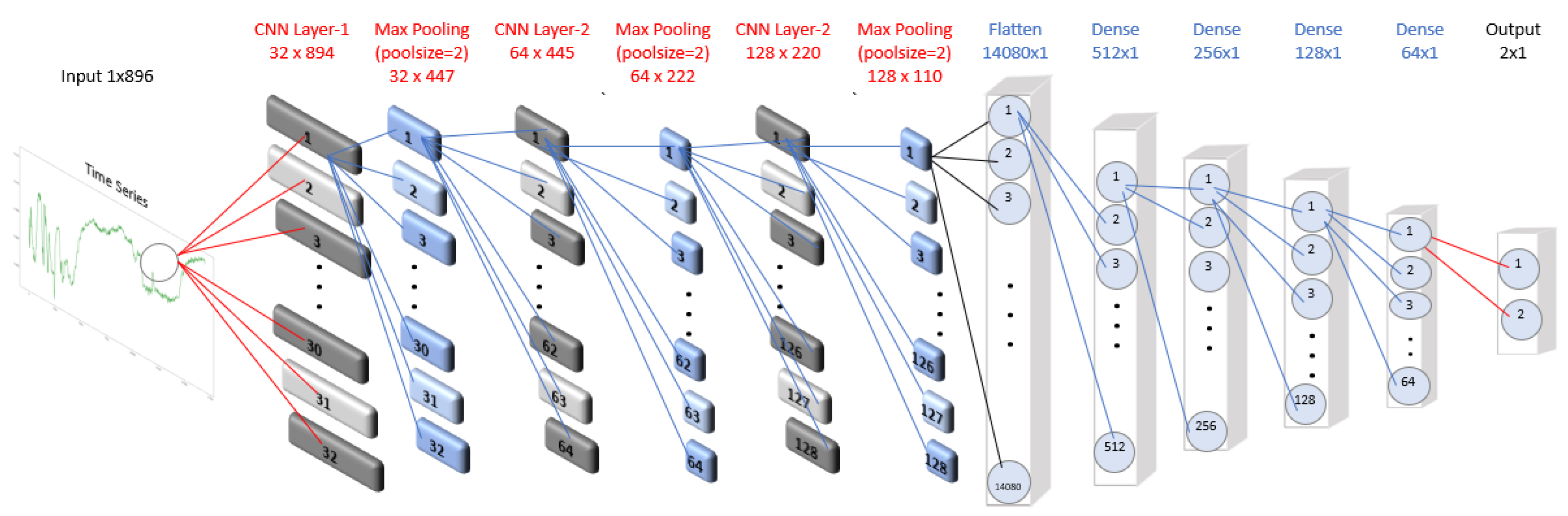
Figure 2.
Plot of mean values for all time series at each time step, segmented by group for the EPI training dataset.
Figure 2.
Plot of mean values for all time series at each time step, segmented by group for the EPI training dataset.
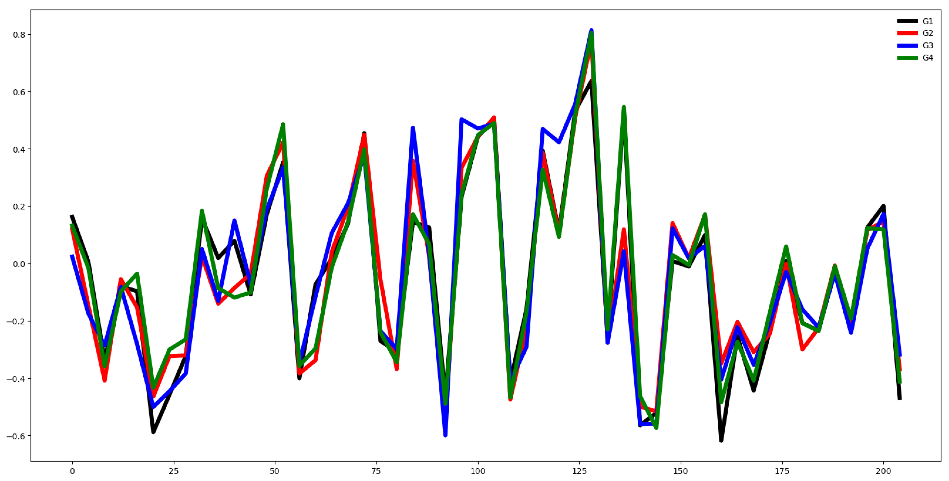
Figure 3.
Plot of mean values of the channels, segmented by group for the EPI training dataset.
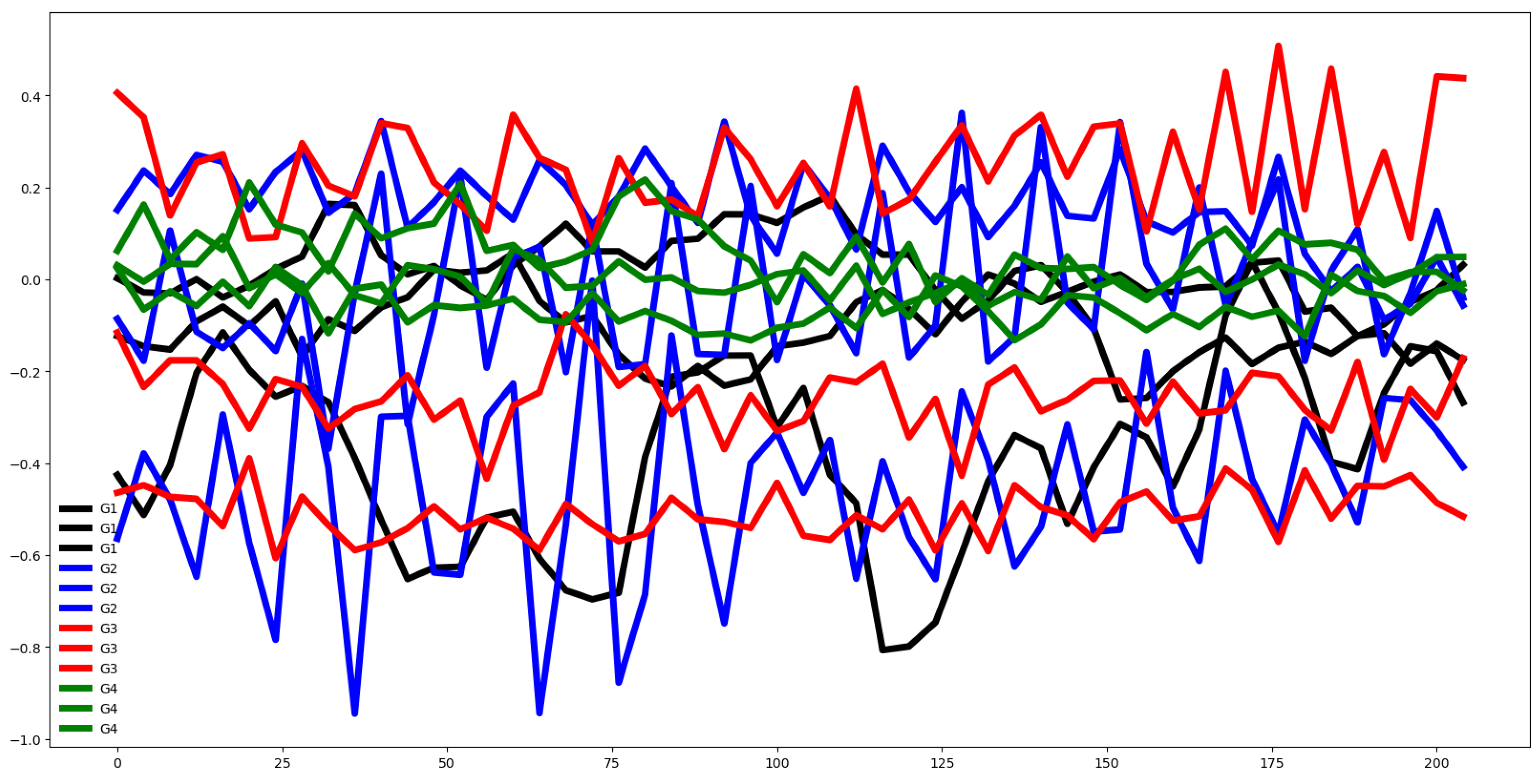
Figure 4.
Boxplots of channels by groups for the (a) training dataset, and (b) testing dataset.
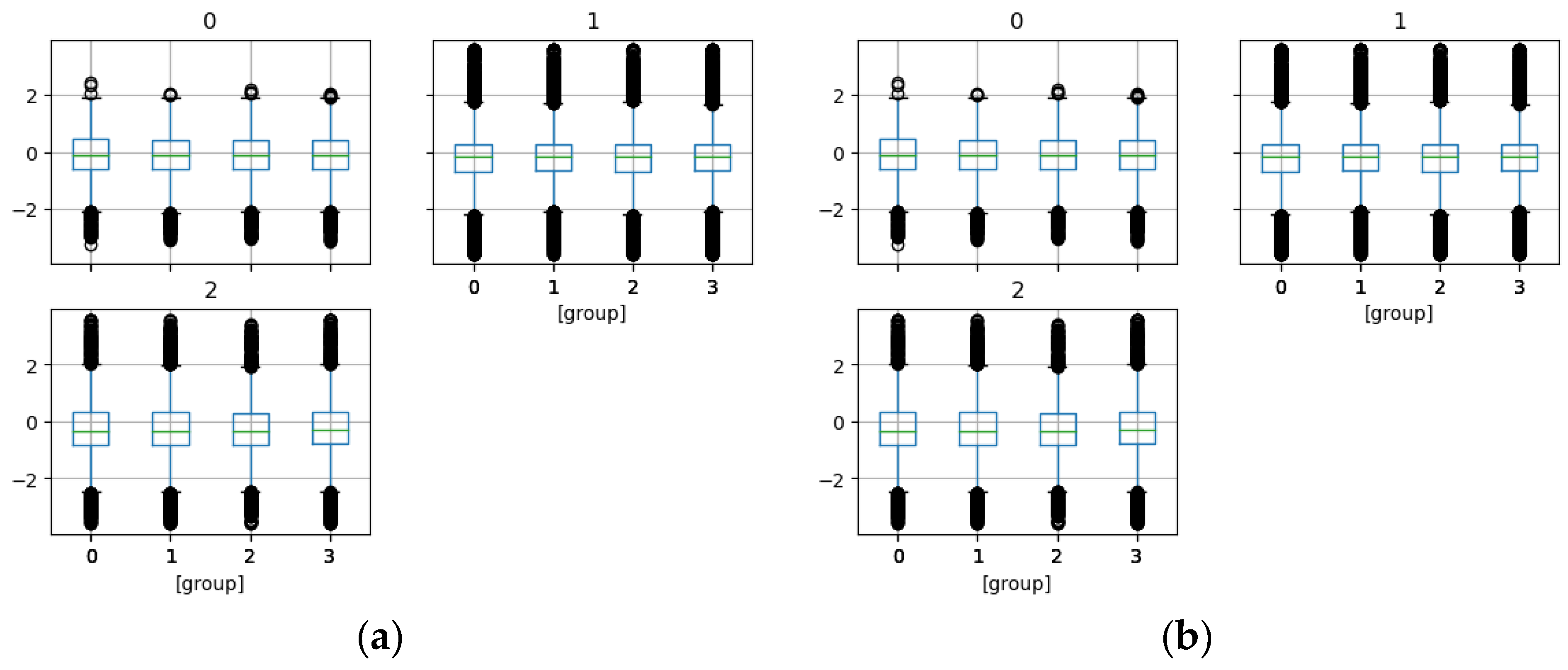
Figure 5.
Plot of mean values of all time series, segmented by group for the EPI training dataset (above) and testing dataset(below).
Figure 5.
Plot of mean values of all time series, segmented by group for the EPI training dataset (above) and testing dataset(below).
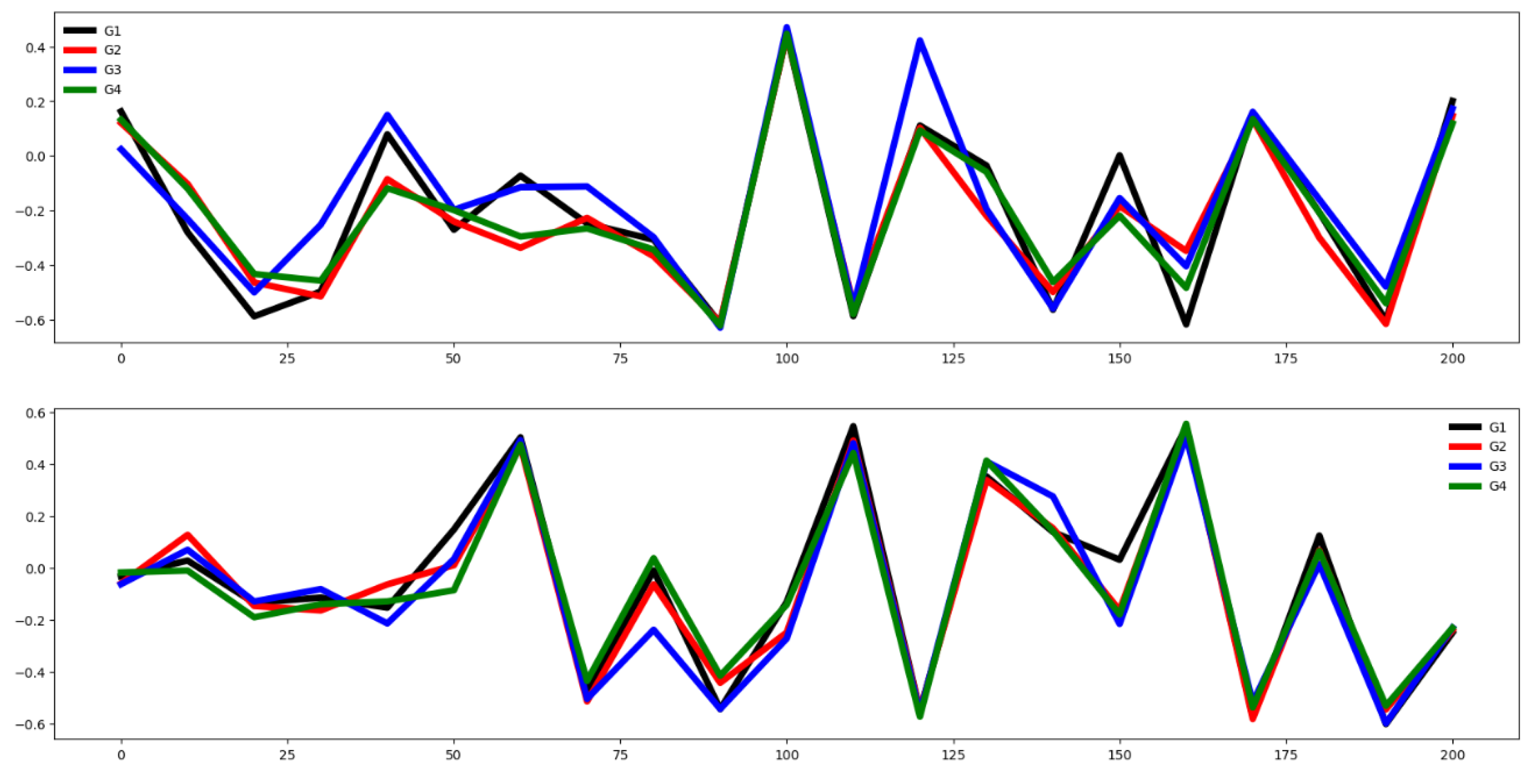
Figure 6.
Plot of mean values for all time series at each time step, segmented by group for the NATOPS training dataset.
Figure 6.
Plot of mean values for all time series at each time step, segmented by group for the NATOPS training dataset.
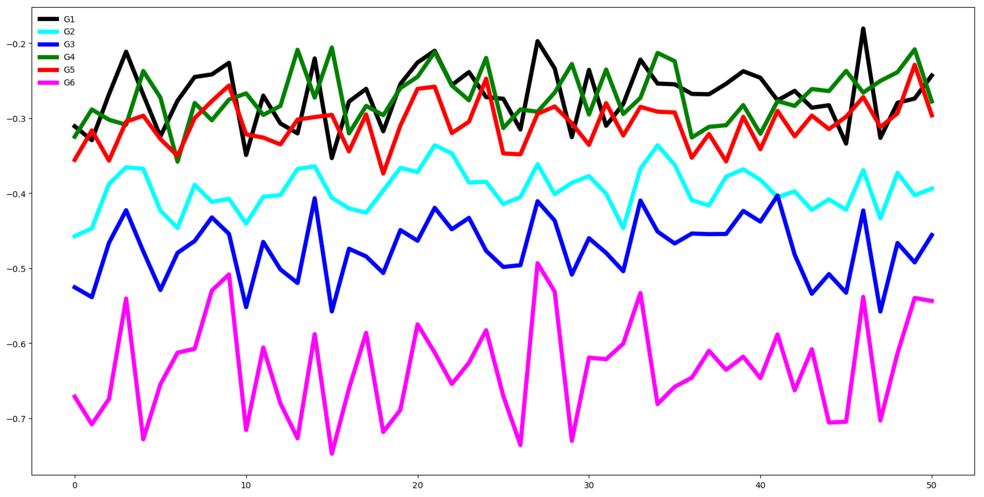
Figure 7.
Plot of mean values by channel, segmented by group for the AWR training dataset.
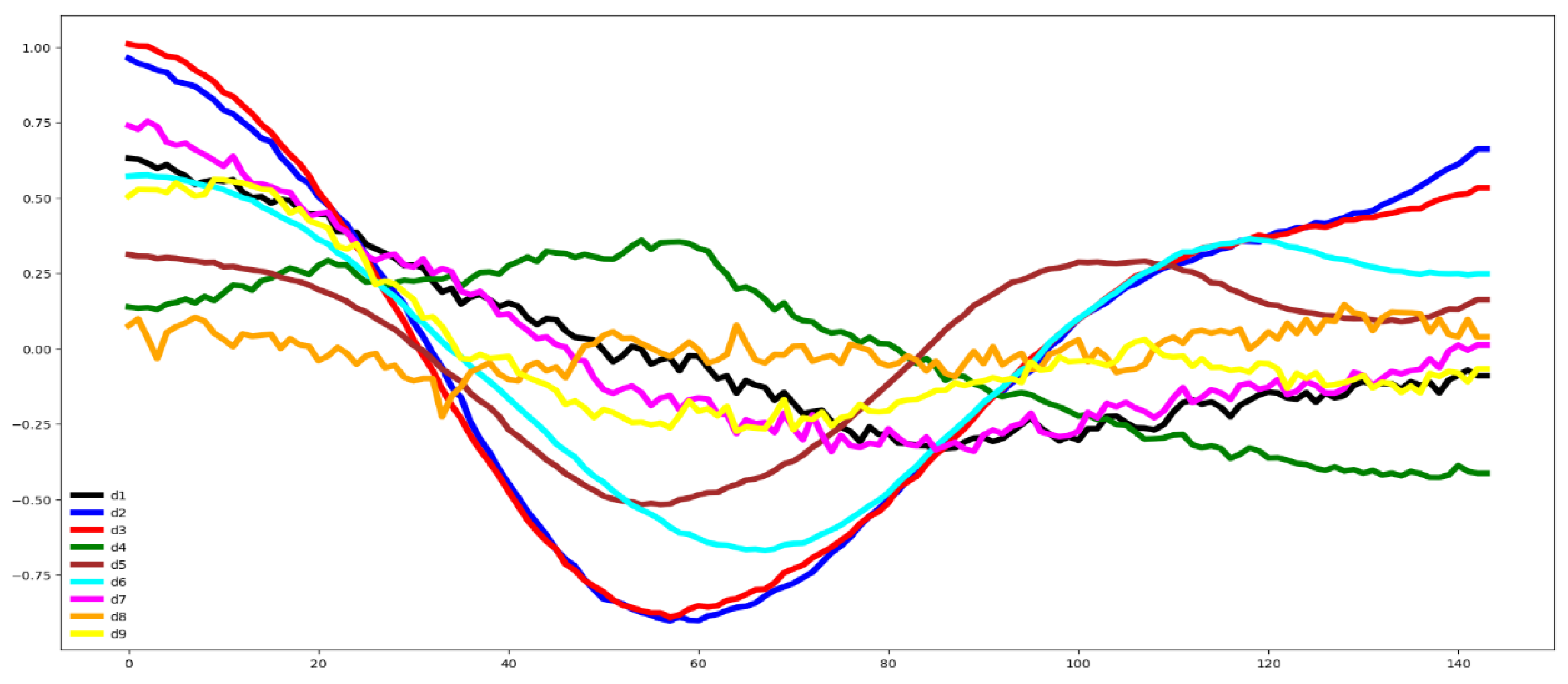
Figure 8.
Plot of mean values by channel, segmented by group for the SCP1 training dataset.
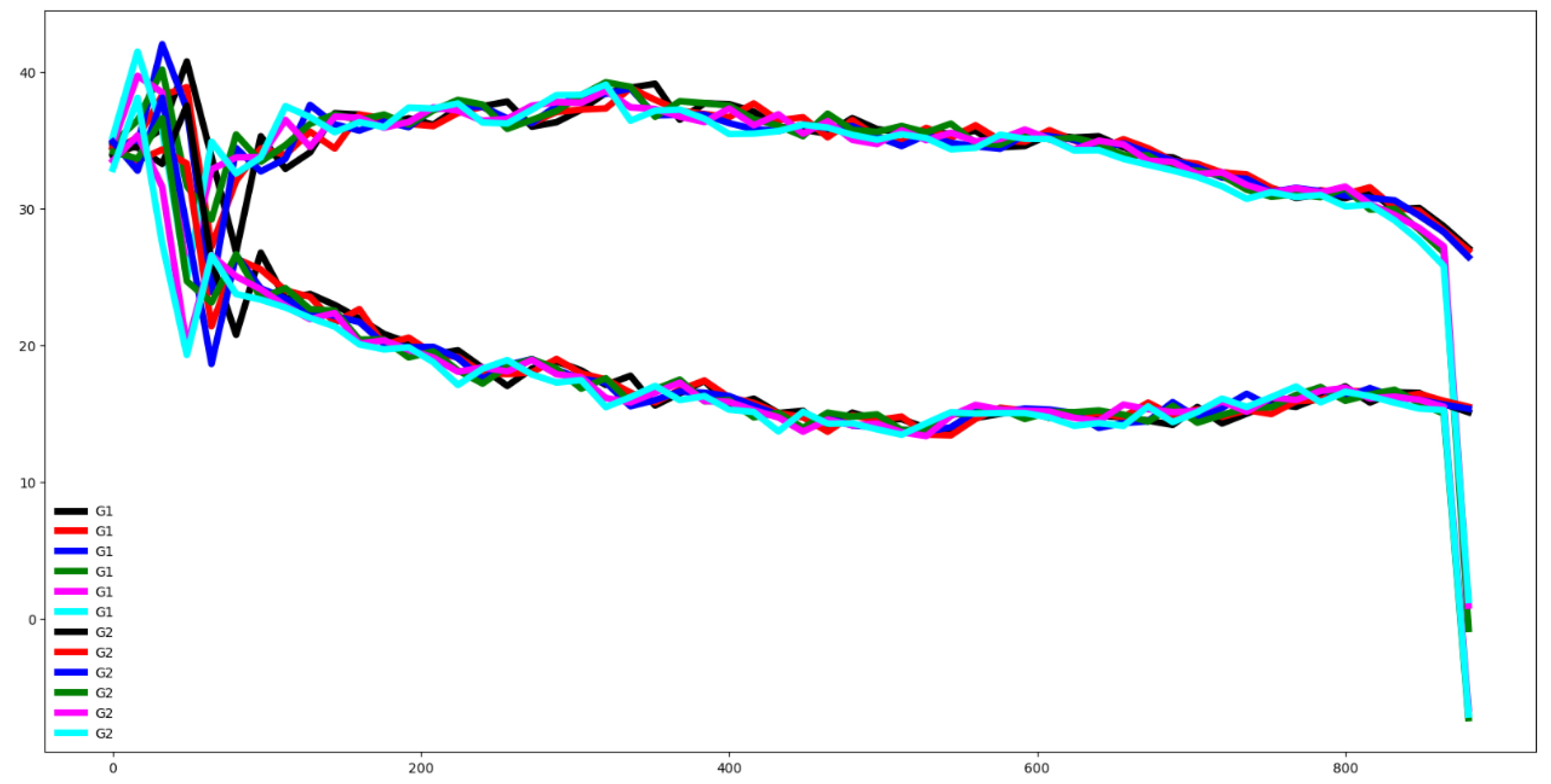
Figure 9.
Plot of mean values for all time series at each time step, segmented by group for the SCP1 training dataset.
Figure 9.
Plot of mean values for all time series at each time step, segmented by group for the SCP1 training dataset.
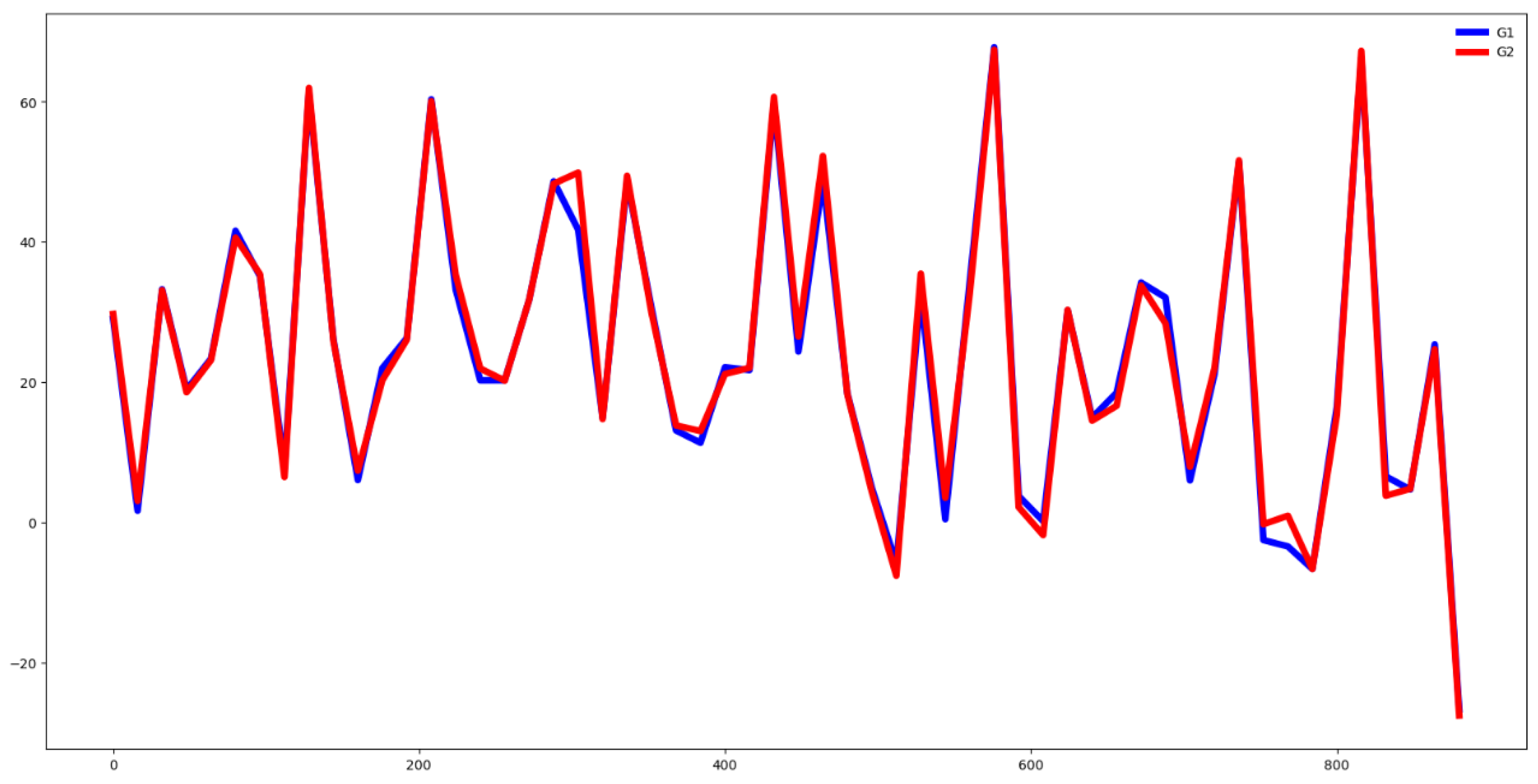
Figure 10.
Plot of mean values for all time series at each time step, segmented by group for the PEMS training dataset.
Figure 10.
Plot of mean values for all time series at each time step, segmented by group for the PEMS training dataset.
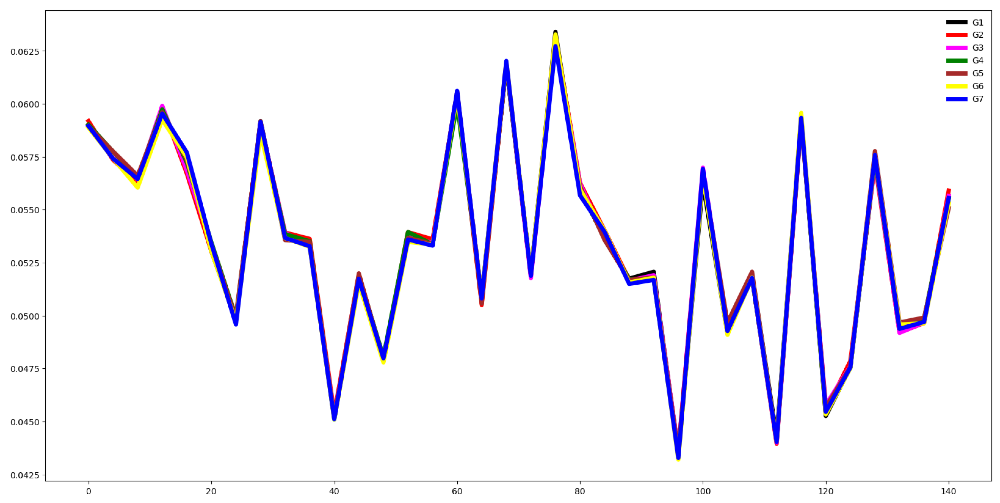
Figure 11.
Plot of mean values of the first 20 channels, segmented by each of the seven groups for the PEMS training dataset.
Figure 11.
Plot of mean values of the first 20 channels, segmented by each of the seven groups for the PEMS training dataset.
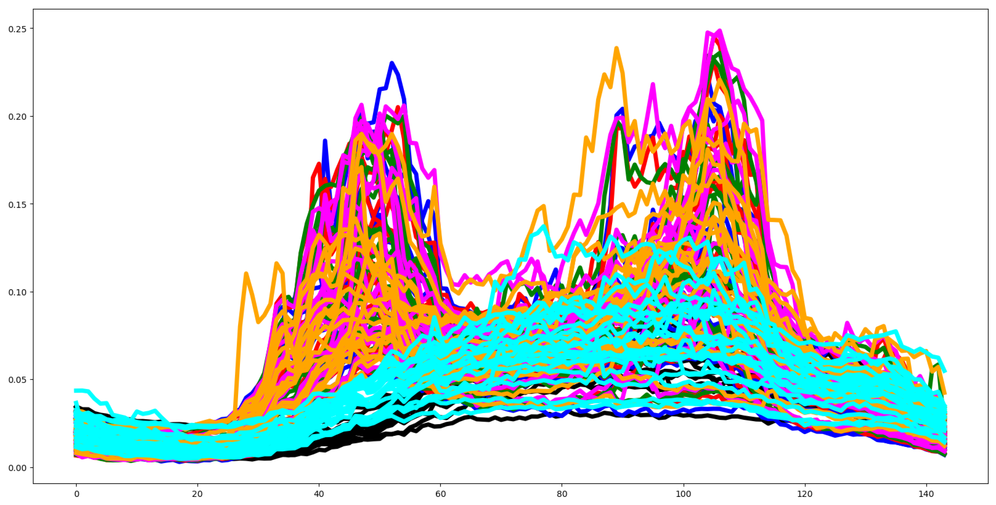
Figure 12.
Plot of mean values by channel, segmented by group for the HB training dataset.
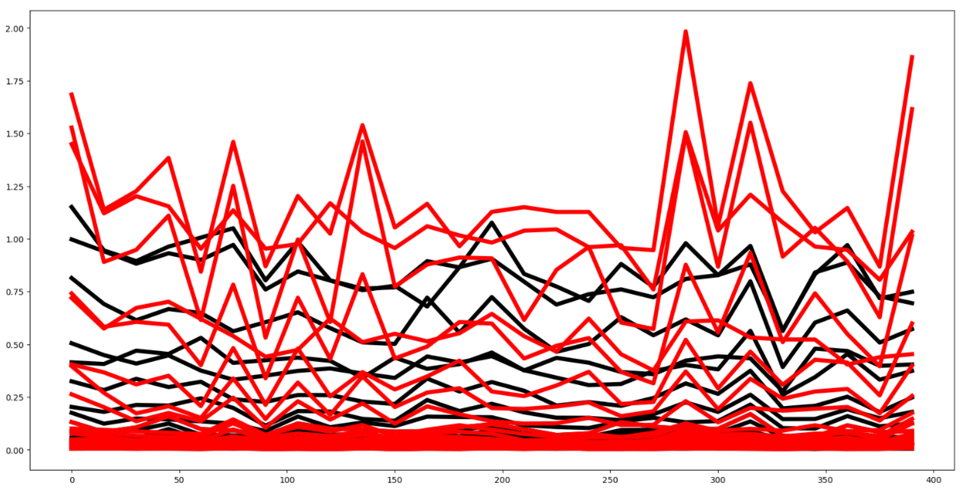
Figure 13.
Plot of mean values of all time series, segmented by group for the HB training dataset (above) and testing dataset (below).
Figure 13.
Plot of mean values of all time series, segmented by group for the HB training dataset (above) and testing dataset (below).
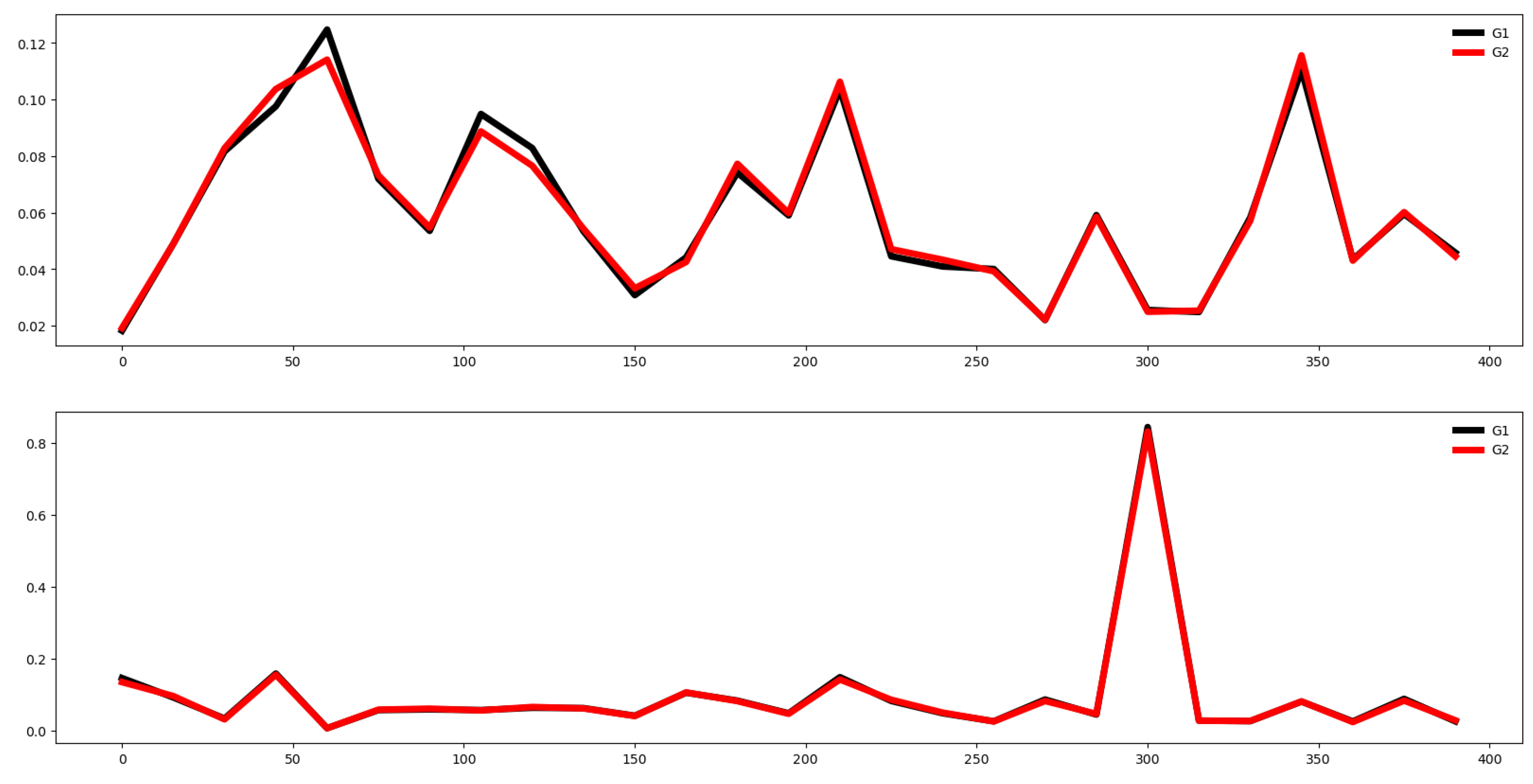
Figure 14.
Plot of mean values of the first 20 channels, segmented by group for the FD training dataset.
Figure 14.
Plot of mean values of the first 20 channels, segmented by group for the FD training dataset.

Figure 15.
Plot of mean values of all time series, segmented by group for the FD training dataset (above) and testing dataset (below).
Figure 15.
Plot of mean values of all time series, segmented by group for the FD training dataset (above) and testing dataset (below).
Figure 16.
Plot of mean values of the first 20 channels, segmented by each of the 5 groups for the DDG training dataset.
Figure 16.
Plot of mean values of the first 20 channels, segmented by each of the 5 groups for the DDG training dataset.
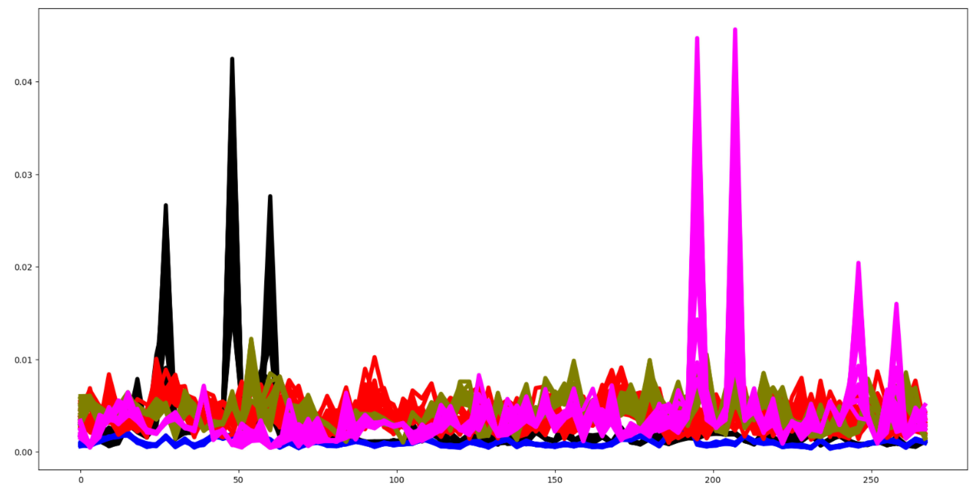
Figure 17.
Plot of mean values of all time series, segmented by group for the DGG training dataset.

Figure 18.
Plot of mean values by channel, segmented by group: G1(Black), G2(red), for the FM training dataset.
Figure 18.
Plot of mean values by channel, segmented by group: G1(Black), G2(red), for the FM training dataset.
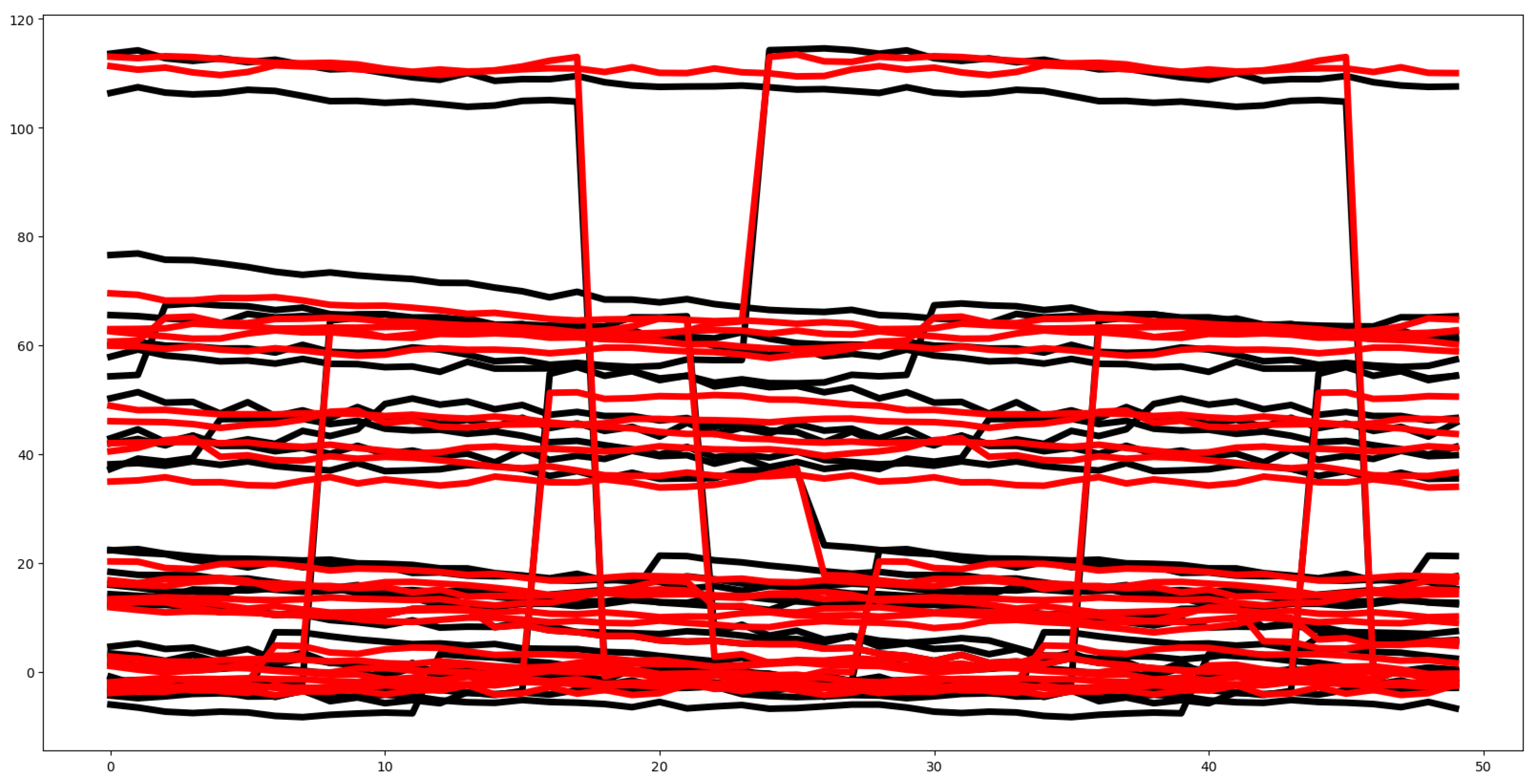
Figure 19.
Plot of mean values of all time series, segmented by group for the FM training dataset.
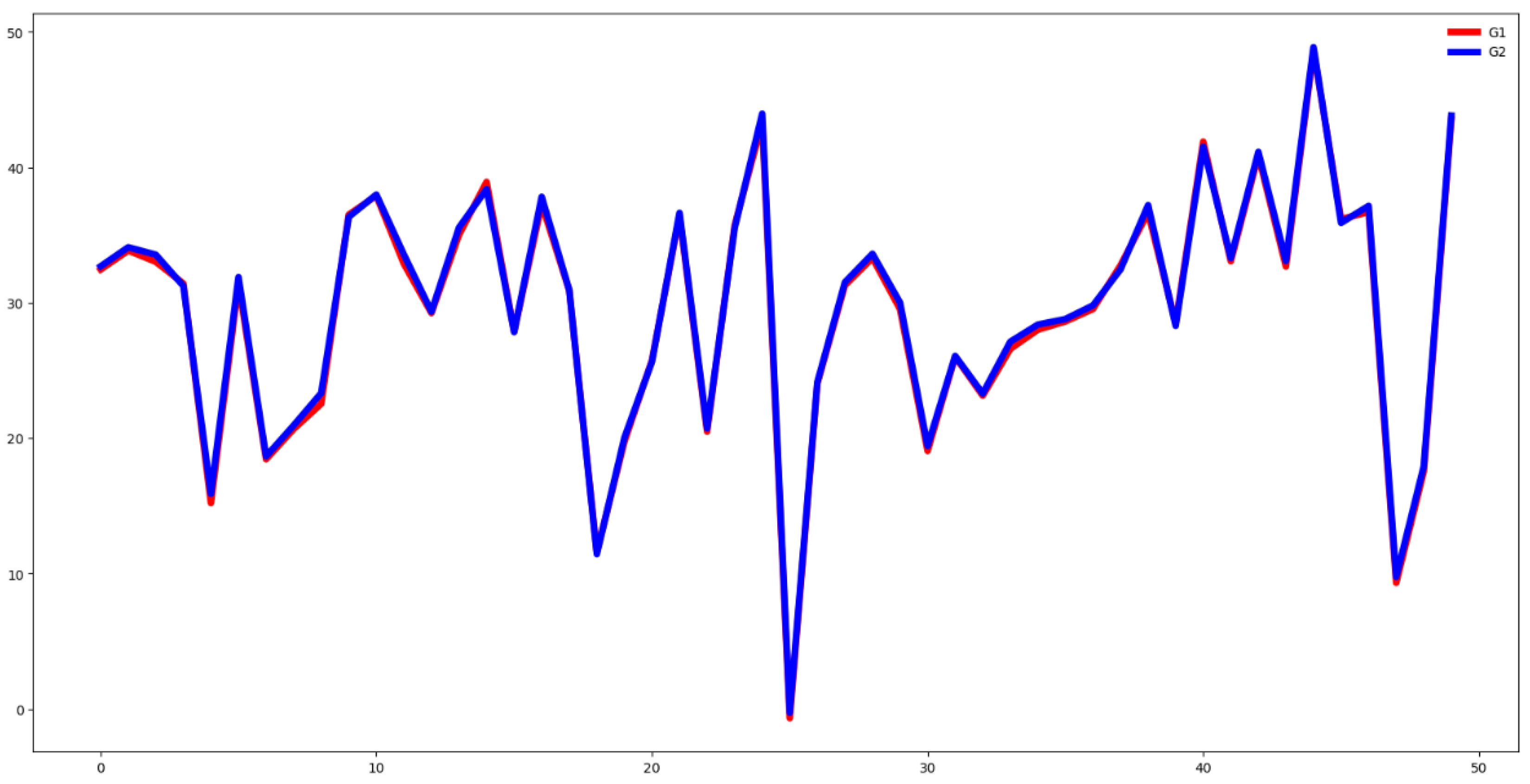
Figure 20.
Plot of mean values by channel across groups for the SCP2 training dataset.
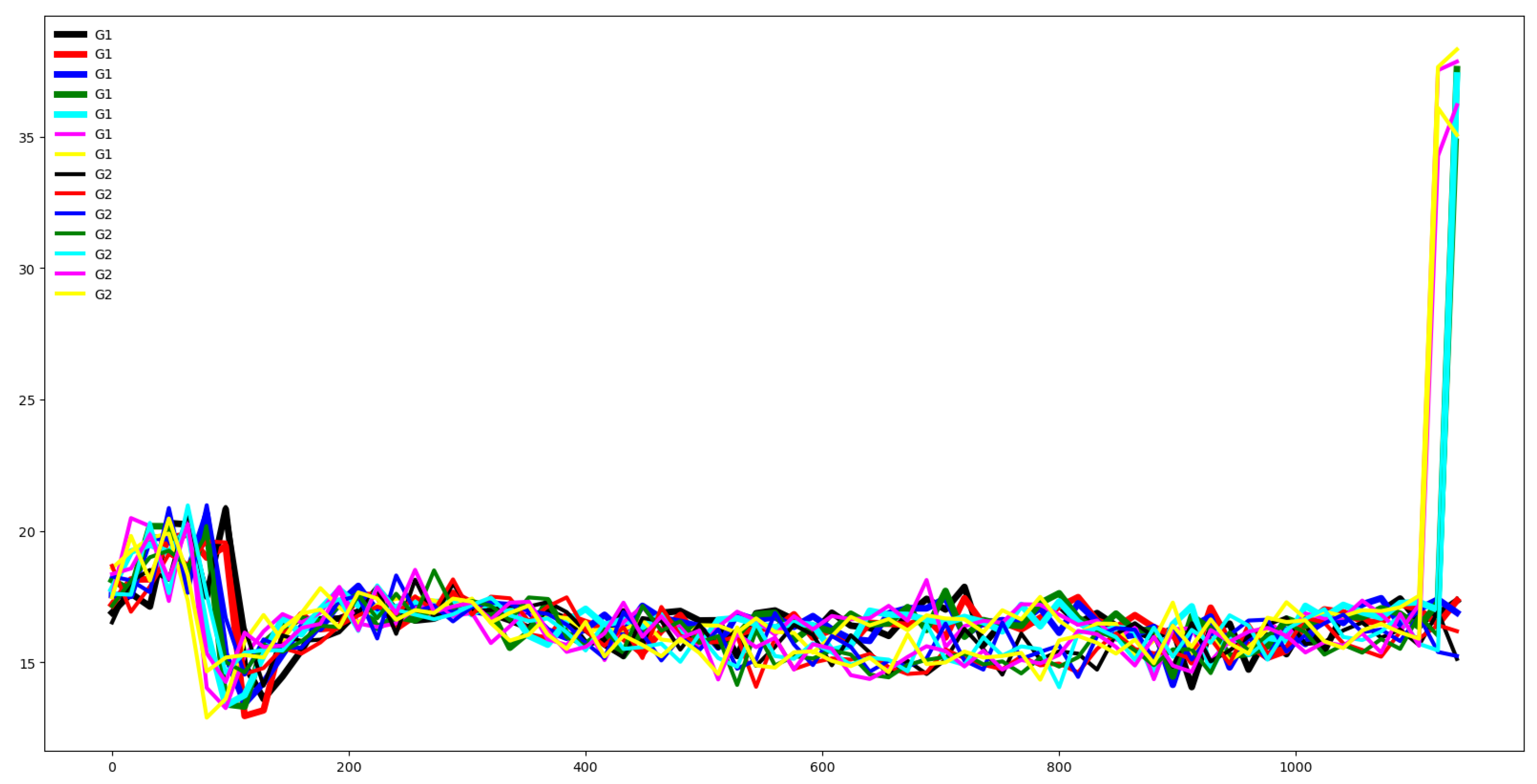
Figure 21.
Plot of mean values of all time series, segmented by group for the SCP2 training dataset.
Figure 21.
Plot of mean values of all time series, segmented by group for the SCP2 training dataset.
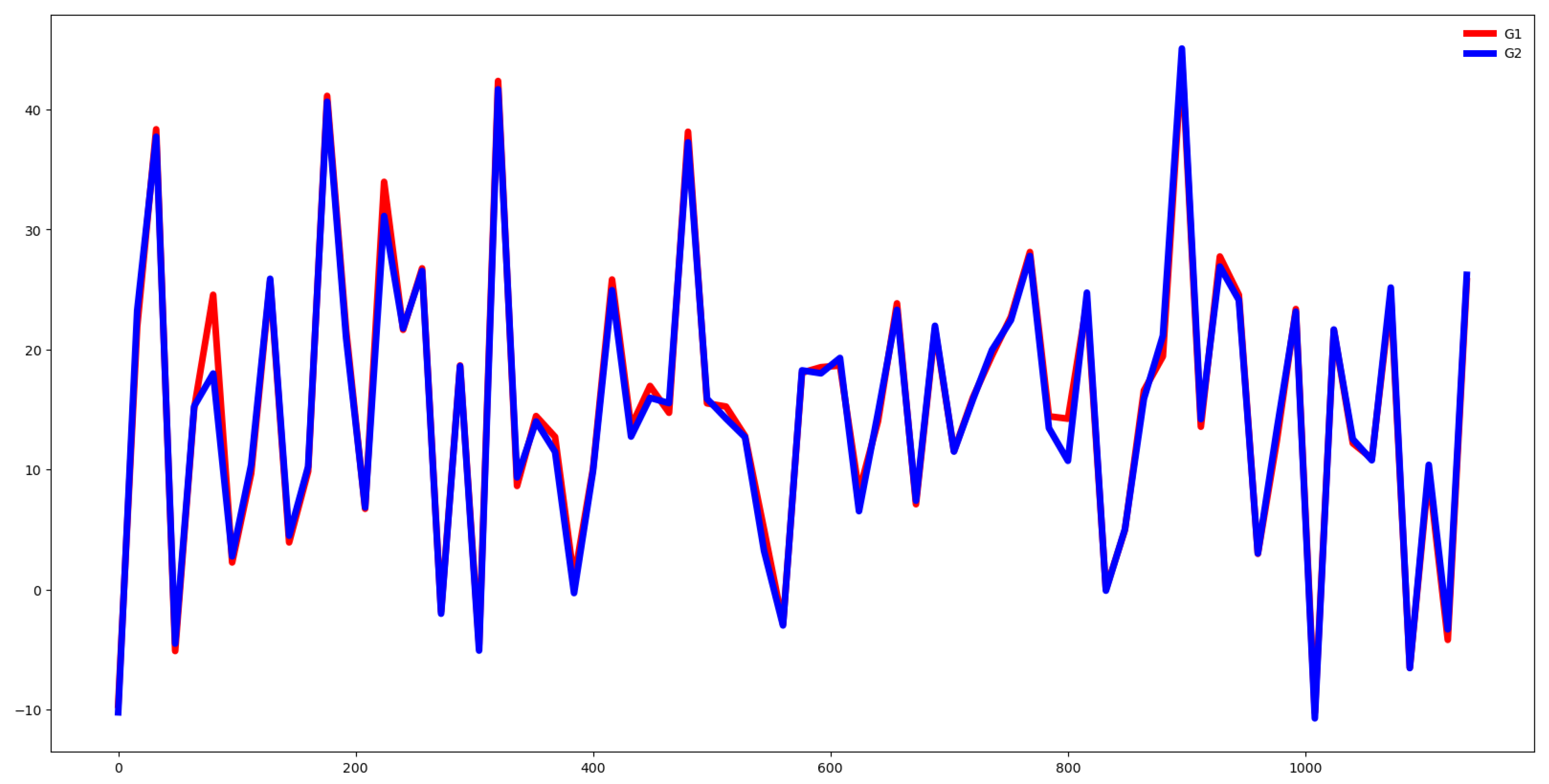
Figure 22.
Plot of mean values of all time series, segmented by channel for the HMD training dataset.
Figure 22.
Plot of mean values of all time series, segmented by channel for the HMD training dataset.
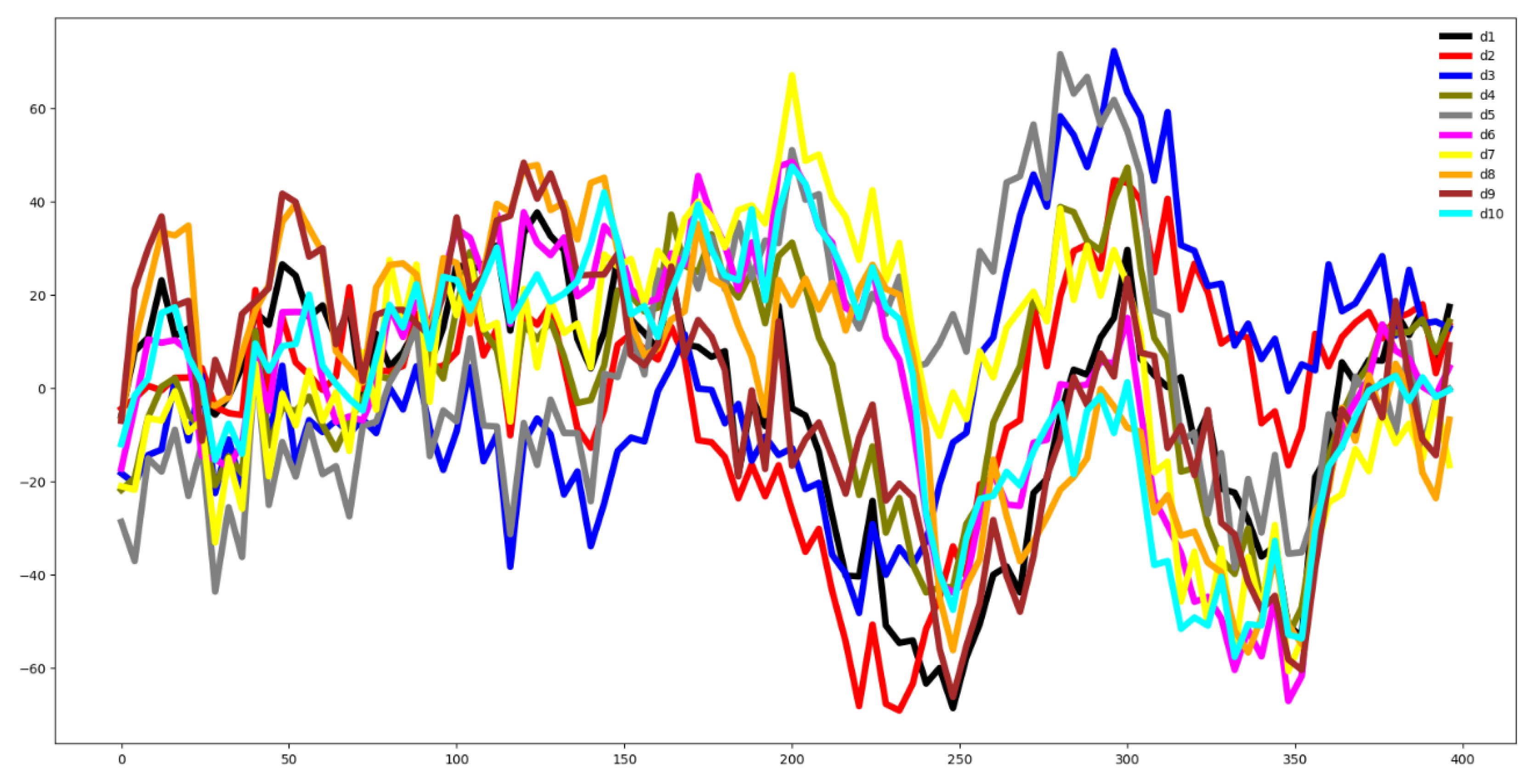
Figure 23.
Plot of mean values of all time series, segmented by group for the HMD training dataset.
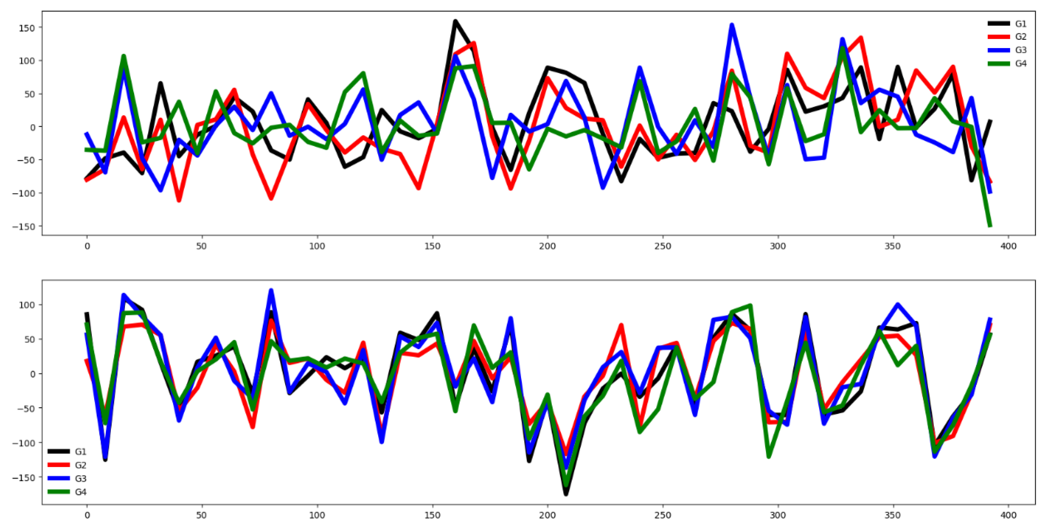
Figure 24.
Plot of mean values by channel across groups for the EC dataset.
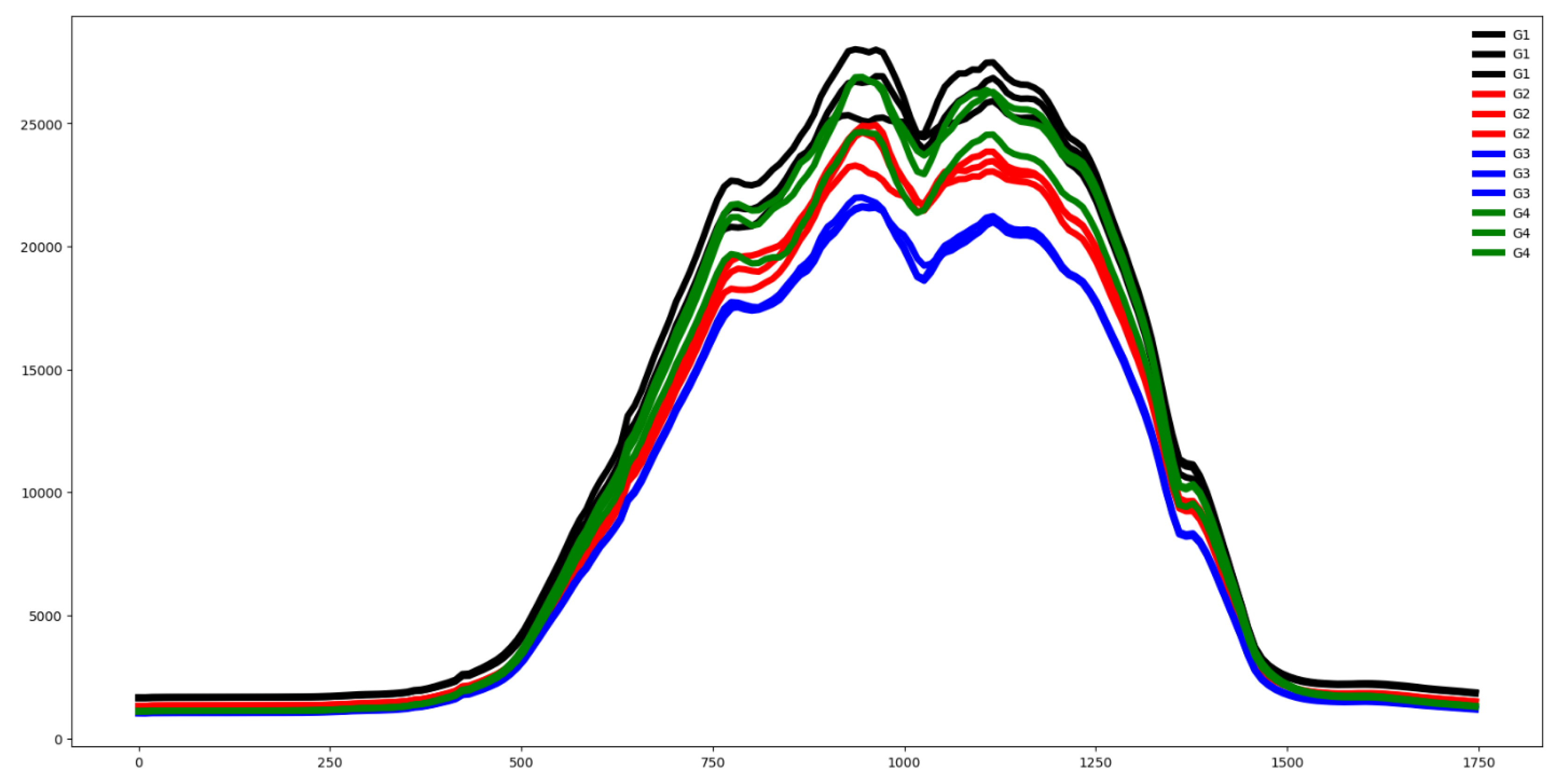
Figure 25.
Plot of mean values of all time series across groups for the EC training dataset (above) and EC testing dataset (below).
Figure 25.
Plot of mean values of all time series across groups for the EC training dataset (above) and EC testing dataset (below).
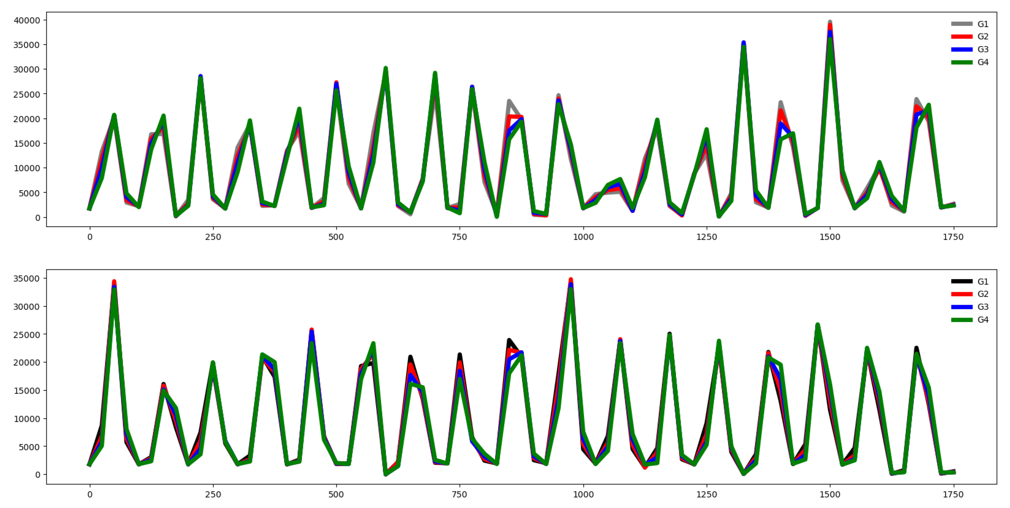

Table 1.
Summary of the datasets considered in the experiments.
| Dataset | Train | Test | Dim(D) | Length | Classes | Train*D | T*D/L | Acc. Default % |
|---|---|---|---|---|---|---|---|---|
| EPI | 137 | 138 | 3 | 206 | 4 | 411 | 1.99 | 26.8 |
| NATOPS | 180 | 180 | 24 | 51 | 6 | 4320 | 84.7 | 26.81 |
| AWR | 275 | 300 | 9 | 144 | 25 | 2475 | 17.18 | 4.00 |
| SCP1 | 268 | 293 | 6 | 896 | 2 | 1608 | 1.79 | 50.2 |
| PEMS | 267 | 173 | 963 | 144 | 7 | 257121 | 1785.5 | 17.34 |
| HB | 204 | 205 | 61 | 405 | 2 | 12444 | 30.7 | 72.19 |
| FD | 5890 | 3524 | 144 | 62 | 2 | 848160 | 13680 | 50.0 |
| DDG | 50 | 50 | 1345 | 270 | 5 | 67250 | 249 | 20.0 |
| FM | 316 | 100 | 28 | 50 | 2 | 8848 | 177 | 51.0 |
| SCP2 | 200 | 180 | 7 | 1152 | 2 | 1400 | 1.22 | 50.0 |
| HMD | 160 | 74 | 10 | 400 | 4 | 1600 | 4 | 40.54 |
| EC | 261 | 263 | 3 | 1751 | 4 | 783 | 0.44 | 25.09 |
| BM | 40 | 40 | 6 | 100 | 4 | 240 | 2.4. | 25.0 |
| RS | 151 | 152 | 6 | 30 | 4 | 906 | 30.2 | 28.3 |
| LIB | 180 | 180 | 2 | 45 | 15 | 360 | 8 | 6.7 |
Table 2.
Accuracy of deep learning classifiers evaluated in the testing set.
| Dataset | LSTM | CNN1D | Transformers | ResNet | Inception Time | Rocket |
|---|---|---|---|---|---|---|
| EPI | 82.53±1.79 | 83.48±1.44 | 76.45±3.33 | 94.05±4.30 | 93.62±5.11 | 99.20±0.79 |
| NATOPS | 83.99±1.69 | 91.67±1.94 | 77.07±5.09 | 92.88±2.68 | 94.27±1.14 | 88.32±0.64 |
| AWR | 87.92±2.09 | 92.93±1.26 | 48.78±3.19 | 93.36±5.70 | 97.56±2.22 | 99.29±0.18 |
| SCP1 | 77.74±1.51 | 78.58±0.73 | 75.63±2.91 | 73.03±6.40 | 76.79±8.80 | 84.88±1.02 |
| PEMS | 89.70±2.22 | 88.55±4.27 | 78.09±2.78 | 73.80±6.95 | 73.86±6.21 | 81.26+/1.44 |
| HB | 71.70±1.21 | 73.56±1.30 | 73.72±2.13 | 57.56±9.77 | 67.36±9.45 | 74.48±0.94 |
| FD | 63.62±0.79 | 61.14±0.46 | 61.38±1.14 | 55.26±1.14 | 65.92±0.94 | 58.67±0.55 |
| DDG | 51.80±5.62 | 62.0±4.42 | 42.6±6.80 | 59.8±4.46 | 61.2±2.35 | 49.4±3.27 |
| FM | 51.79±3.18 | 51.80±2.09 | 50.4±3.02 | 53.6±4.14 | 55.2 ± 2.82 | 55.1±1.28 |
| SCP2 | 53.93±2.67 | 52.72±1.84 | 51.94±2.80 | 51.10±1.75 | 52.77±2.79 | 55.16±2.06 |
| HMD | 34.99±7.63 | 48.78±3.08 | 34.59±3.99 | 30.4±3.89 | 40.80±1.89 | 50.89±3.57 |
| EC | 26.92±1.90 | 27.65±1.52 | 27.97±2.35 | 27.63±2.18 | 28.09±2.79 | 40.83±1.88 |
| BM | 91.49±6.02 | 96.00±2.23 | 62.99±13.96 | 97.0±6.70 | 55.2 ± 2.82 | 100.0±0.00 |
| RS | 74.60±3.24 | 69.99±4.57 | 44.91±12.85 | 88.68±2.0 | 88.28±1.35 | 91.17±0.59 |
| LIB | 16.22±1.59 | 14.79±2.29 | 9.68±1.13 | 81.66±10.51 | 87.44±0.63 | 90.55±0.39 |
Disclaimer/Publisher’s Note: The statements, opinions and data contained in all publications are solely those of the individual author(s) and contributor(s) and not of MDPI and/or the editor(s). MDPI and/or the editor(s) disclaim responsibility for any injury to people or property resulting from any ideas, methods, instructions or products referred to in the content. |
© 2025 by the authors. Licensee MDPI, Basel, Switzerland. This article is an open access article distributed under the terms and conditions of the Creative Commons Attribution (CC BY) license (http://creativecommons.org/licenses/by/4.0/).
Copyright: This open access article is published under a Creative Commons CC BY 4.0 license, which permit the free download, distribution, and reuse, provided that the author and preprint are cited in any reuse.


