
Submitted:
30 October 2025
Posted:
31 October 2025
You are already at the latest version
Abstract
This paper uses visualization techniques to analyze the learning process of six machine learning classifiers for multichannel time series classification (MTSC), including five deep learning models—1D CNN, CNN-LSTM, ResNet, InceptionTime, and Transformer—and one non-deep learning method, ROCKET. Sixteen datasets from the UEA multivariate time series repository were employed to assess and compare classifier performance. To explore how data characteristics influence accuracy, we applied channel selection, feature selection, and similarity analysis between training and testing sets. Visualization techniques were used to examine the temporal and structural patterns of each dataset, offering insight into how feature relevance, channel informativeness, and group separability affect model performance. The experimental results show that ROCKET achieves the most consistent accuracy across datasets, although its performance decreases with a very large number of channels. Conversely, the Transformer model underperforms in datasets with limited training instances per class. Overall, the findings highlight the importance of visual exploration in understanding MTSC behavior and indicate that channel relevance and data separability have a greater impact on classification accuracy than feature-level patterns.
Keywords:
multichannel time series classification
; multivariate time series classification
; UEA archive
; time series visualization
; deep learning classifiers
1. Introduction
Multichannel or multivariate time series classification (MTSC) involves assigning labels to temporal sequences in which each instance contains multiple synchronized measurements recorded over time. Each measurement captures one aspect of a complex system, and together they provide a richer representation than univariate time series. These measurements are called channels or dimensions. In a multichannel time series, each observation consists of dimensions measured across aligned time steps. For an instance , we denote where for . When , the dataset corresponds to a univariate time series. Here, y is an integer-valued variable representing the groups or classes. MTSC tasks arise in diverse domains, including healthcare, human activity recognition, environmental monitoring, and industrial process control, where understanding temporal dependencies across multiple sensors or modalities is essential for accurate classification.
Recent advances in deep learning have significantly improved MTSC performance. Convolutional neural networks (CNNs), recurrent neural networks (RNNs), and attention-based architecture such as Transformers have shown strong potential for capturing temporal and cross-channel relationships. At the same time, non-deep approaches such as the Random Convolutional Kernel Transform (ROCKET) have demonstrated competitive or even superior accuracy with much lower computational cost. Despite this progress, it remains challenging to determine which algorithm performs best under different data characteristics—such as the number of channels, time-series length, or inter-class similarity. Moreover, visualization-based analyses of classifier behavior remain scarce, limiting our understanding of why models succeed or fail on specific datasets.
This study addresses these gaps by integrating visualization and quantitative analysis to examine the learning behavior of six representative classifiers: CNN-1D, LSTM , ResNet, InceptionTime, Transformer, and ROCKET. Using sixteen datasets from the UEA multivariate time series archive, we evaluate how input structure and data properties affect classification accuracy. In particular, we analyze the influence of channel relevance, feature selection, and train–test similarity on model performance. Visualization techniques are employed to explore patterns in channel-wise and feature-wise behavior, providing interpretable insights into each classifier’s strengths and limitations. We also evaluated the stationarity of the time series in each dataset, as it may impact classification outcomes.
Our findings reveal that ROCKET consistently achieves strong and stable performance across most datasets, although its accuracy decreases with very high channel dimensionality. Conversely, the Transformer model underperforms in datasets with few training instances per class. More broadly, our results suggest that channel informativeness and group separability exert a greater impact on MTSC accuracy than feature-level variations.
2. Related Work
Research on multichannel or multivariate time series classification (MTSC) has advanced rapidly with the development of standardized repositories and deep learning architectures. Bagnall et al. [1,2] introduced and later expanded the UEA MTSC archive. Their studies compared several traditional and ensemble methods but reported aggregate rather than dataset-specific results, leaving open questions about model behavior across varying data characteristics.
Fawaz et al. [3] conducted a comprehensive review of deep learning models for time series classification. They also explored visualization techniques, including Class Activation Maps (CAMs), and Multi-Dimensional Scaling (MDS), which shows the spatial distribution of input time series among the classes. However, these tools were primarily applied to univariate datasets, and their analyses did not address how channel relevance or feature separability affect multichannel performance.
Subsequent works have examined alternative representations and feature-based approaches. For, instance, Baldan and Benítez [4] proposed a MTSC method using 41 descriptive features that capture inter-channel relationships, evaluated on all 30 UEA datasets with classical algorithms such as Random Forest and SVM. Pasos Ruiz et al. [5] expanded this line of research by benchmarking 16 algorithms, including deep and non-deep methods, on 26 multivariate datasets. Their work provided valuable aggregate comparisons but did not analyze visual or structural factors influencing classifier accuracy.
More recently, Pasos Ruiz and Bagnall [6] investigated dimension-reduction and channel-selection strategies within the HIVE-COTE v2.0 ensemble framework, while Ilbert et al. [7] implemented data augmentation strategies to compensate for limited training data; however, the resulting performance gains were marginal.
Despite these efforts, few studies have systematically examined how visualization, feature relevance, and channel informativeness jointly influence classifier performance in MTSC tasks. The present work extends prior research by combining visualization-driven interpretation with quantitative channel and feature selection analyses across 16 datasets from the UEA repository. In addition, this study contrasts five deep learning models with the non-deep ROCKET algorithm, providing a clearer understanding of the relationship between data structure and model accuracy.
3. Materials and Methods
3.1. Classification Algorithms
To evaluate the performance and interpretability of representative approaches for multichannel time series classification (MTSC), six algorithms were selected. These include five deep learning models—One dimensional CNN, LSTM, ResNet, InceptionTime, and Transformer—and one non-deep method, ROCKET. Together they capture the principal paradigms used in MTSC research: convolution-based, recurrent, attention-based, and kernel-based learning. All models were implemented using publicly available code within the sktime framework [9] and trained under comparable hyperparameter settings to ensure fairness across datasets. HIVE-COTEv2, a heterogeneous meta-ensemble for MTSC, was excluded due to scalability issues with high-dimensional or long time series data [5]. Other ensemble approaches were omitted for similar reasons. The following subsections provide brief overviews of each classifier.
3.1.1. The Random Convolutional Kernel Transform (ROCKET)
Introduced by Dempster et al. [8], represents a fast, non-deep learning alternative that transforms time series into high-dimensional feature spaces using thousands of randomly generated convolutional kernels. For each kernel, two statistics—the maximum value and the proportion of positive values (PPV)—are extracted and used to train a linear classifier such as ridge or logistic regression. This approach achieves high accuracy with minimal parameter tuning and scalability to large datasets. The multivariate extension randomly assigns kernels to channels, aggregating responses across dimensions to form a fixed-length representation.
For each of the 10,000 kernels, parameters are sampled as follows: The kernel length is selected such that, ; the weight, , in the kernel is selected such that, ; dilation is drawn from an exponential distribution scaled to the input length; and padding is applied with 50% probability. When padding is enabled, zeros are added symmetrically to both ends of the time series, ensuring that the kernel’s center aligns with all time-step positions.
The convolution between each time-series instance and a kernel can be interpreted as a dot product, generating a feature map from which two statistics are extracted: the maximum value and the proportion of positive values (PPV). The PPV quantifies the fraction of the series that is positively correlated with the kernel and has been shown to enhance classification accuracy. After applying all convolutions, each series is represented by a 20 000-dimensional feature vector, which is subsequently used to train a ridge regression classifier.
A multivariate extension of ROCKET is available in Python’s sktime library [9]. In this version, kernels are randomly assigned to channels, with weights generated per channel. Convolution operates as a matrix dot product across channels, and the maximum and PPV values are computed jointly over all dimensions for each kernel, producing a 20 000-dimensional feature representation. Ridge regression is typically employed due to its efficiency in tuning the regularization parameter through cross-validation. However, for very large datasets where the number of instances greatly exceeds the number of features, logistic regression optimized via stochastic gradient descent offers better scalability. Overall, ROCKET transforms each time series into a high-dimensional feature space, analogous to the kernel mapping performed by Support Vector Machines (SVMs).
3.1.2. Residual Network (ResNet)
ResNet was first introduced for time series classification by Wang et al. [10]. It consists of sequential convolutional blocks connected through identity shortcuts that facilitate gradient flow and mitigate vanishing-gradient issues. A global average-pooling and soft-max layer perform final classification. ResNet serves as a baseline for evaluating deep convolutional architectures in time series applications. In this study, we use the same hyperparameters and optimizer settings as in Fawaz et al. [3], with implementation provided through the sktime interface to their original code [9].
3.1.3. InceptionTime
InceptionTime [12] extends the ResNet by incorporating Inception modules that apply convolutions of multiple lengths in parallel, enabling the model to detect patterns at different temporal scales. An ensemble of five networks with independently initialized weights enhances robustness and stability. Each network includes two blocks, each containing three Inception modules, unlike ResNet’s three blocks of standard convolutional layers. In similar way to ResNet, these blocks use residual connections and conclude with global average pooling and a soft-max layer.
3.1.4. One Dimensional Convolutional Neural Network (CNN-1D)
Numerous CNN architectures—such as LeNet, AlexNet, and GoogleNet [13]—have been employed for multivariate time series classification. In this work, we implemented a sequential 1D Convolutional Neural Network (CNN-1D) model [14,15], which is particularly well-suited for analyzing sequential data such as time series and spectral data. In the CNN-1D model, each time series is represented by the input shape parameter of the Conv1D layer, defined by the number of feature maps (filters) and the kernel size. The number of feature maps determines how many distinct representations of the input are learned, while the kernel size specifies the number of time steps considered when generating each feature map.
In our experiments, the number of feature maps was varied between 32 and 256, with kernel sizes of 2 or 3. Each Conv1D layer was followed by a MaxPooling1D layer with a pool size of 3, and this block was repeated three times. A flatten layer was then added, followed by three fully connected (dense) layers with 64 neurons each. The output layer matched the number of dataset classes and employed the softmax activation function. Because most datasets contained a limited number of features, we did not include a dropout layer. The architecture of the CNN-1D model used for the SCP1 dataset is illustrated in Figure 1. The model was trained for 300 epochs with a batch size of 256, optimizing the categorical cross-entropy loss function using the Adam optimizer, a variant of stochastic gradient descent.
3.1.5. LSTM
In a Multilayer Perceptron (MLP), each neuron is fully connected to the neurons of adjacent layers, with no intra-layer connections. In contrast, a Recurrent Neural Network (RNN) incorporates a weighted sum of previous inputs into the hidden layer’s computation, enabling it to account for both the current input and prior outputs [16]. This recurrent feedback mechanism allows the network to capture temporal dependencies and contextual information, making RNNs well-suited for sequential data such as time series and spectral signals.
However, standard RNNs suffer from short-term memory limitations, making it difficult to retain information over long sequences. Long Short-Term Memory (LSTM) networks, a specialized type of RNN, overcome this issue by introducing gating mechanisms that control the flow of information [17,18]. These gates enable the network to decide which information to retain, update, or forget, allowing LSTMs to effectively model long-term dependencies and improve predictive performance across extended sequences.
3.1.6. Transformers
Vaswani et al. [19] introduced attention-based neural networks—known as Transformers—originally developed for natural language processing (NLP) tasks, where word sequences follow grammatical and syntactic order. In a Transformer model, an input sequence (e.g., text in English) is mapped to an output sequence (e.g., text in Spanish). When applied to time series analysis, where data are chronologically ordered in time steps, the Transformer predicts future values along the temporal axis based on prior observations. Owing to its ability to capture long-range dependencies and complex interactions, the Transformer architecture has proven highly effective for time series modeling, often outperforming RNN and LSTM models in various applications [20,21,22].
A defining characteristic of the Transformer is its use of attention heads, which learn dependencies between each time step and all others within the input sequence. The model dynamically adjusts attention weights to emphasize relevant temporal relationships while diminishing less important ones, with a score matrix representing the strength of association among time steps.
The Transformer architecture comprises stacked Encoder and Decoder layers, each incorporating Embedding layers for their respective inputs. The final output layer produces the model’s predictions. Within each attention block, key components include a Self-Attention mechanism, Layer Normalization, and a Feed-Forward network, where the input and output dimensions of each block are identical.
3.2. Datasets
This study uses 16 out of the 30 MTSC datasets from the UEA repository [1]. Several datasets were excluded for specific reasons. Four of them—Insect Wingbeats, Spoken Arabic Digits, Character Trajectories, and Japanese Vowels—were omitted due to unequal time series lengths, which would require preprocessing that could bias classifier comparisons. Another four—AtrialFibrillation, ERing, StandWalkJump, and BasicMotions—have fewer than 50 training instances, which poses challenges for deep learning models. However, BasicMotions was retained to assess model behavior on small datasets.
Four datasets—Libras, LSST, PendDigits, and RacketSports—contain very short time series (fewer than 50 time steps), which may limit the effectiveness of machine learning models. Of these, we included Libras and RacketSports. In contrast, EigenWorms and MotorImagery have extremely long time series (over 2,000 time steps), which can burden models and degrade accuracy. While binning could reduce dimensionality, we excluded these datasets to ensure fair comparisons. The Phoneme dataset was also omitted due to its small training set and large number of classes (39), which could hinder classifier performance.
Lastly, the Handwriting and UWaveGesture datasets were excluded due to their small training sets relative to the size of their test sets. This imbalance, combined with low training set dimensionality, tends to result in poor performance for deep learning models.
Table 1 provides a summary of these datasets, arranged in descending order of mean accuracy obtained in our experiments. In the first column, among parenthesis, appears the reference for each dataset. The Train × Ch and Train × Ch/L metrics are used as proxies for data complexity. It is evident the Face Detection (FD) is the most complex dataset. The last column represents the baseline random accuracy in percentage. For instance, in the AWR dataset this accuracy is , since . For the EPI dataset the default accuracy is since , 37 is the largest group size in the training set of the dataset.
3.3. Research Workflow
We have applied two filter methods to select relevant features in time series: the F-test and the Mutual Information criterion. The F-test for a given feature assesses the ratio of between-group to within-group variance. Features with higher F-test values are considered more relevant for classification. Given the high dimensionality of the data, we compute p-values for each feature using the F-test and then transform them into scores using the negative logarithm. A feature is deemed relevant if its normalized score—defined as is greater than , a threshold chosen for practical effectiveness.
The second method, Mutual Information, quantifies the statistical dependence between each feature and the class labels. Features with higher mutual information scores are more informative. These scores are also normalized by dividing each by the maximum score, and features with a normalized value above 0.5 are selected as relevant.
For channel selection, we use the method implemented in the sktime library, based on the approach proposed by Dhariyal et al. [34]. This method represents each class using a prototype time series and evaluates channels based on the distance between these class prototypes. Channels contributing to greater separation between classes are considered more informative.
Some UEA datasets are not pre-normalized. For these, we apply z-score normalization to the training set: . The test set is normalized using the mean and standard deviation computed from the training data.
In order to establish separability among the time series between groups in the training set, first we computed the averaged time series for each group, where , N stands by the number of groups. Here, we used:
where L is the number of timestamps of the time series and is the number of time series in the group G. After that, we compute both the Euclidean distance and the Dynamic Time Warping (DTW) distance between the averaged time series of the groups.
The DTW distance between two time series, and , is defined as the minimum total cost of an optimal warping path that aligns the sequences. This optimal path, found using dynamic programming, starts at and ends at with each step calculated recursively using:
The starting distance is taking as .
DTW is an algorithm designed to align and compare two time series. Unlike other methods that compare points strictly by their position in the sequence, DTW emphasizes similarities in the overall shape of the data. In this paper we have used the Python’s library dtaidistance [35] to compute the DTW distance.
Our research workflow diagram is shown in Figure 2:
4. Results
4.1. Classifiers Accuracy Results
Table 2 reports the mean and standard deviation of test accuracy across ten independent runs for each dataset–algorithm pair. ROCKET employed 20,000 random kernels. ResNet and InceptionTime were trained for 300 and 200 epochs, with batch sizes of 16 and 64, respectively. CNN-1D, LSTM, and Transformer models were trained for 300 epochs with a batch size of 32. All experiments were conducted in Python 3.10.9 using scikit-learn, Keras, and TensorFlow 2.0.
The highest-performing results for each dataset are highlighted in bold. In cases of statistically indistinguishable performance, multiple algorithms are bolded. To assess statistical significance, pairwise comparisons among classifiers were performed using the non-parametric Wilcoxon signed-rank test.
Across the sixteen datasets, ROCKET achieved the highest accuracy in eleven cases, confirming its robustness and scalability for multichannel time series. Its performance was particularly strong on medium-sized datasets such as Cricket, Basic Motions, Epilepsy, and AWR, where clear inter-class separation and moderate channel counts favored convolutional kernel representations. CNN-1D obtained competitive or best performance in six datasets, indicating that shallow convolutional models can rival deeper architectures when temporal patterns are locally structured. InceptionTime produced solid results on four datasets, benefiting from its multi-scale convolutions but showing sensitivity to limited training data.
Conversely, Transformer and LSTM-based models tended to underperform, especially in datasets with few instances per class (AWR, DDG) or very short sequences (LIB, RS). Their accuracy improved only in larger, more regular datasets such as PEMS-SF and Heartbeat, where longer temporal context was beneficial. ResNet consistently ranked among the lowest-performing architectures, likely due to overparameterization relative to dataset size.
Overall, the Wilcoxon analysis confirmed that ROCKET outperformed the remaining algorithms at a 5% significance level in most pairwise comparisons. Among deep learning methods, CNN-1D showed no statistically significant difference from ROCKET on several small- and mid-scale datasets, highlighting its efficiency and generalizability.
When aggregating results across all sixteen datasets, ROCKET obtained the highest mean test accuracy (≈ 82%) and the lowest standard deviation (≈ 1.8%), indicating strong stability. CNN-1D and InceptionTime followed with mean accuracies of approximately 77% and 74%, respectively. LSTM and Transformer models achieved lower averages near 63%, while ResNet presented the lowest overall mean accuracy, below 60%. Based on average ranks across datasets, ROCKET placed first, CNN-1D second, and InceptionTime third. These results demonstrate that shallow convolutional or kernel-based methods remain competitive—even against modern deep architectures—particularly when training data are scarce, or channel dimensionality is high.
Collectively, these outcomes underscore that data dimensionality and sample size are dominant determinants of classifier effectiveness. Models emphasizing convolutional feature extraction (ROCKET, CNN-1D, InceptionTime) adapt better to medium-length, multichannel series, whereas attention- or recurrence-based networks require substantially more training instances to achieve comparable performance.
These findings suggest that data dimensionality and sample size critically determine classifier performance. Models emphasizing convolutional feature extraction (ROCKET, CNN-1D, InceptionTime) adapt better to multichannel data with moderate sequence length, whereas attention- and recurrence-based architectures require substantially more training examples to achieve comparable accuracy. These trends motivated the subsequent visual analyses presented in Section 4.2, aimed at understanding how channel relevance and feature separability explain the observed performance differences.
4.2. Discussion of Individual Dataset Results
This section provides visual and quantitative analyses of feature and channel behavior across datasets. Feature selection results are also reported for each training set: the F-test was applied to normalized datasets, whereas the Mutual Information criterion was used for unnormalized data. Due to space constraints, some figures have been omitted but are available for download at github.com/eacunafer.
In each dataset we have computed several measures. First, the percentage of relevant channels. Second, the percentage of the relevant features using both the F-test and the Mutual Information criterion. Third, we present the minimum Euclidean distance as well as the DTW distance between the averaged time series by group. These minimum of these distances are taken to have an idea of the degree of groups separation. Finally, we present the mean DTW distance between the groups in the training and testing sets in a pairwise way. This last score is computed to measure the similarity between training and testing sets in each dataset. All the results are summarized in Table 3.
4.2.1. Cricket (CRI)
In the Cricket dataset, the unnormalized time series values range from -10 to 12. As shown in Figure 3, most of the six channels exhibit distinct group-wise mean curves with minimal overlap, indicating high discriminative potential across classes. The sktime channel selection method corroborates this observation, identifying all six channels as relevant (Table 3). In contrast, both feature selection techniques applied in this study—the F-test and the Mutual Information criterion—highlight that only a small proportion of individual features contribute significantly to classification. However, there is a good separation distance among the mean time series by groups in the training set (See Table 3). Also, Figure 4 validates this assertion. The training and testing datasets behave somehow similarly, as illustrated by their mean time series by group in Figure 4. Together, these visualizations suggest that classifier performance in this dataset is influenced more by the channel relevance than feature relevance.
4.2.2. Basic Motions (BM)
In the Basic Motions dataset, unnormalized time series values range from -30 to 35. As illustrated in Figure 5, only the first three channels appear to be the most relevant for classification, with minimal overlap between group-wise mean curves. This claim agrees with the result obtained by the channel selection method (see Table 3). According to the distances between the mean time series group, shown in Table 3, there is a good separation among the groups in the training set. This assertion is also supported by Figure 6. On the other hand, the training and testing datasets exhibit similar distributions as shown in Figure 6. These observations indicate that, in the BM dataset, classifier performance is more influenced by informative channels and strong similarity between training and testing sets than by feature patterns.
4.2.3. Epilepsy (EPI)
Figure 7 presents the group-wise mean time series for each channel, showing that only the third channel exhibits clear class-discriminative patterns, while the remaining channels display substantial overlap among groups. This conclusion agrees totally with the one obtained using the channel selection criterion (see Table 3). However, the feature selection methods do not report a high percentage of relevant features (see Table 3). Figure 8 further illustrates the group-wise mean time series across the training and testing datasets, highlighting consistent temporal patterns between training and testing data. A clear separation is observed among the four mean time series curves, suggesting some features are highly informative. Together, these visualizations suggest that classifier performance in this dataset is influenced by channel and feature relevance as well as similarity between training and testing sets.
4.2.4. NATOPS
As shown in Figure 9, in this dataset many channels demonstrate relevance for classification, evidenced by the limited overlap among group-wise mean time series curves. This claim agrees with the high percentage of relevant channels for NATOPS shown in Table 3. In the same table it is shown that a reasonable percentage of features are considered relevant. Figure 10 shows that there is a good separation between the mean time series for all six groups in both the training and testing datasets. These observations indicate that, in the NATOPS dataset, classifier performance is more influenced by informative channels than by feature patterns as well as a good similarity between training and testing sets.
4.2.5. Articulacy Word Recognition (AWR)
As shown in Figure 11, up to five channels appear to be clearly relevant for the classification task. Despite this, the channel selection method from sktime identifies all nine channels as relevant (see Table 3). Channel selection results may be affected by the presence of outliers that may reduce the test’s sensitivity. In each channel there is a substantial overlap among the group-wise mean time series curves. Also, in Table 3, we can see a low percentage of relevant features and a modest separation between the mean time series by group in the training set. The training and testing sets also show highly similar feature behavior. These findings suggest that, in this dataset, classification performance depends more on channel-specific patterns than on individual feature behavior. The Transformer’s performance is hindered by the dataset’s imbalance between the large number of classes (25) and the small number of instances per class (11). Excluding the Transformer, this dataset produced the highest classification accuracy overall. Notably, applying channel selection via the sktime library did not improve Transformer results.
4.2.6. Racket Sports (RS)
In this dataset, unnormalized time series values range from -35 to 35. As shown in Figure 12, most of the six channels appear relevant for classification. The channel selection method identifies 66.67% of channels as important (see Table 3). Figure 13 shows a clear separation among the group-wise time series in the training dataset. The training and testing datasets exhibit similar behavior, as illustrated in the same figure. Together, these visualizations suggest that classifier performance in this dataset is influenced by channel and feature relevance as well as a high similarity between training and testing sets.
4.2.7. PEMS-SF
The dataset includes 963 channels, representing a high-dimensional multivariate structure. Figure 14 shows only the first 20 channels, and we can see some degree of separation among the mean time series of the seven groups. The channel selection method identifies only 33.02% out of 963 channels as important (see Table 3). There is only a small separation between the mean time series by group in the training set. Also, we can notice that there is some similarity between the training and testing distributions as reflected by the averaged time series of the seven groups. This last fact can help the classifier performance for this dataset.
4.2.8. SelfRegulationSCP1 (SCP1)
The unnormalized time series values in this dataset range from -75 to 125. As shown in Figure 15, there is clear separation between group-wise mean time series values across most of the 6 channels throughout the time series, except at the initial segment of the signals. Despite this, the channel selection method identifies only three channels (50%) as relevant. Figure 16 shows a good separation in mean time series values across groups in the training set. Once again, both feature selection methods report a very low percentage of relevant features. These claims suggest that channel-level information may be more influential than feature-specific patterns in driving classifier performance. Furthermore, a substantial difference exists between the training and testing sets based on the behavior of their averaged time series by group. This indicates significant distributional dissimilarity, which may impact model generalization.
4.2.9. Libras (LIB)
In the Libras dataset, the data is normalized. As shown in Figure 17, both channels appear relevant to the classification task. Figure 17 suggests that both channels are informative for classification. Despite only moderate separation among the group-wise mean time series, a considerable number of features demonstrate discriminative power. In the same figure, the training and testing datasets exhibit some similarity of their averaged time series by group. These claims suggest that both channel-level information feature-specific patterns help classifier performance. In addition to that, it is also worth noting that the time series are very short, containing only 45 time steps. This last fact hurts the performance of Deep Learning classifiers.
4.2.10. Heartbeat (HB)
The training set is imbalanced, containing 147 instances in one class and 57 in the other, a disparity that negatively impacts classifier performance. Figure 18 shows substantial overlap in channel-wise mean values across the two groups, indicating that only a few channels are useful for classification. Consistently, the channel selection method from the sktime library identifies just 14.75% of channels as relevant (see Table 3). Figure 19 illustrates the averaged time series by group for both training and testing data. Based on that, the feature pattern behavior between training and testing sets seems to differ considerably. Also, there is a very small separation between the mean time series by groups in both sets. These factors may explain the moderate accuracy achieved by the classifiers on this dataset.
4.2.11. Face Detection (FD)
Figure 20 shows some overlap in the mean time series across groups for the first 20 channels, indicating limited group separation. The channel selection method available from the sktime library identifies only 8.33% of the 144 channels as relevant for classification (see Table 3). The testing dataset exhibits a strong resemblance to the training dataset. Also, there is a very small separation between the mean time series by groups in the training set as well as the testing set. This justifies the low percentage of relevant features. Together, these findings suggest that achieving high classification accuracy on this dataset may be inherently challenging due to the limited discriminative information available.
4.2.12. Duck Duck Geese (DDG)
This dataset is characterized by extremely high dimensionality, with 1,345 channels, and exhibits substantial overlap in the mean time series across the five groups in most channels. According to the channel selection method only 28.77% of the channels are relevant for classification. Additionally, the training set is relatively small, containing only 50 instances, 10 of them in each of the 5 groups. Some mean time series include pronounced spikes or outliers within specific ranges, as shown in Figure 21. There is a limited separation in the averaged time series by groups of the training set. Also, we can see that the training and testing sets differ notably. The small number of instances hampers the performance of the Transformer model. Attempts to mitigate this limitation through data augmentation using autoencoders were not successful. Overall, classification on this dataset is particularly challenging due to limited discriminative channel information, differences in the probabilistic distribution between training and test sets, and the presence of outliers in the training set.
4.2.13. SelfRegulationSCP2 (SCP2)
This dataset is like the SCP1 dataset but differs from it in that it contains a greater number of timestamps and one additional channel. The data is unnormalized, with training time series values ranging from -35 to 120. As shown in Figure 22, there is substantial overlap in the mean time series across channels for both groups, and only three channels appear visually relevant. However, the channel selection method identifies five relevant channels, 71.4% of the total. There is minimal separation between the averaged time series by group. Additionally, there is a notable distributional shift between training and testing data. These factors collectively suggest that this dataset presents a substantial classification challenge due to weak class separability, minimal feature relevance, and a pronounced mismatch between training and testing distributions.
4.2.14. Finger Movements (FM)
The unnormalized time series values in this dataset range from -170 to 200. Figure 23 shows that most channel-wise mean time series display significant overlap across groups. The channel selection method implemented in the sktime library identifies only 21.42% of the 28 channels as relevant for classification (see Table 3). Also, there is a very small separation between the mean time series by groups in the training set. Additionally, there is a high distributional shift between training and test data. It is also worth noting that the time series are very short, containing only 50 time steps. All of the factors mentioned above contribute to the suboptimal performance of classifiers on this dataset.
4.2.15. Hand Movement Direction (HMD)
The unnormalized time series values in this dataset range from -750 to 1000. As shown in Figure 24, there is considerable overlap among several channel-wise mean curves across groups, suggesting that most of the channels may carry limited discriminative information for classification. The channel selection method applied in this study identifies only 20% of channels as relevant (see Table 3). In Figure 25, we can see distinguish clearly the mean time series corresponding to the four groups in the training dataset. Also, a different mean time series group behavior between the training and testing sets can be observed. These factors along with a limited feature relevance (see Table 3) contribute to reduced classifier performance on this dataset.
4.2.16. Ethanol Concentration (EC)
This dataset is unnormalized, with time series values ranging from 0 to 25,000. It has a very number of timestamps. As shown in Figure 26, the group-wise mean time series are distinguishable across all three channels—particularly in the middle portion of the signal—suggesting that all channels contribute meaningfully to classification. This observation aligns with the channel selection results from the sktime method, which also identifies all three channels as relevant. In Figure 27, we can notice a fair separation between the mean time series by groups. Also, we can see that the distributional similarity between the training and testing datasets is relatively low. This suggest that the different behavior of the training and testing sets make classification a difficult task.
The visual analyses presented above reveal that classifier performance in multichannel time series classification is largely governed by the structural properties of the data rather than by architectural complexity alone. Datasets exhibiting clear class separability, a high proportion of informative channels, and strong alignment between training and testing distributions consistently yielded higher accuracies across models. Conversely, datasets with substantial inter-set divergence or a surplus of weakly relevant channels produced unstable or degraded results, regardless of the algorithm employed. These findings establish a direct link between the visual metrics and quantitative outcomes discussed in Section 4.1 and provide the empirical basis for the conclusions outlined in the following section.
5. Conclusions
In this study, visualization techniques were employed to identify datasets that pose particular challenges for classification and to examine whether classifier performance is more strongly influenced by channel-level behavior or feature-level patterns. Overall, satisfactory performance was achieved primarily in the first six datasets listed in Table 1, Table 2 and Table 3. The results indicate that the proportion of selected channels exerts a greater influence on classification accuracy than the proportion of selected feature patterns. An exception appears in the EC dataset, where high dissimilarity between the training and testing sets degraded classifier performance. Across all classifiers, accuracy declined in datasets with a small number of instances per class, whereas greater separability among group-wise mean time series—whether at the channel or feature level—was associated with improved performance, as evidenced by the comparison between the SCP1 and SCP2 datasets, both from the same domain.
Additional observations reinforce these findings. Classifier performance diminished in cases of substantial distributional differences between the training and testing data, such as in the FM and HMD datasets. The Transformer model was particularly affected by datasets with few instances per class (e.g., AWR and DDG), while deep learning classifiers underperformed on datasets containing very short time series, such as RS and LIB.
There was substantial agreement between the visualization and the channel selection method in establishing the percentage of relevant features. Lack of concordance was observed only in the CRI, AWR, PEMS, SCP1, and SCP2 datasets.
Our accuracy results align closely with those reported in the literature, particularly by Pasos Ruiz [5]. However, we obtained superior results on three datasets: HMD, Heartbeat, and SCP2. Among the algorithms evaluated, ROCKET demonstrated the highest overall performance, followed by CNN-1D, whereas Transformer and ResNet models showed lower effectiveness. ROCKET’s performance declined in datasets with a large number of channels, such as PEMS, FD, and DGG.
Some limitations in the use of visualization arise when dealing with a large number of channels, groups, or timestamps. Therefore, it is advisable to apply dimensionality reduction techniques before visualization. We also recommend performing channel selection prior to feature selection. Computation time increased significantly with longer time series and higher dimensionality, particularly in the DDG, FD, and PEMS datasets. For the Transformer model, computation time also scaled with the number of instances.
Taken together, these findings highlight the importance of considering both data characteristics and methodological choices in multivariate time series classification. Variations in stationarity, class distribution, and dimensionality were shown to strongly influence classifier performance, underscoring the need for careful dataset analysis prior to model selection. While ROCKET and CNN-based approaches demonstrated robust performance across many conditions, no single algorithm consistently outperformed others in all scenarios. Future research should explore integrated approaches that combine visualization, channel selection, and feature selection, as well as the development of more adaptive models capable of handling high-dimensional and heterogeneous time series data.
Supplementary Materials
The computing code used in this work and additional figures can be downloaded at https://github.com/eacunafer.
Author Contributions
Conceptualization, E.A.; methodology, E.A.; software, E.A. and R.A; validation, E.A. and R.A.; formal analysis, E.A.; investigation, E.A.; resources, E.A. and R.A.; data curation, E.A.; writing—original draft preparation, E.A.; writing—review and editing, R.A.; visualization, E.A. and R.A.; supervision, X.X.; project administration, E.A. All authors have read and agreed to the published version of the manuscript.
Funding
This research received no external funding.
Institutional Review Board Statement
Not applicable.
Informed Consent Statement
Not applicable.
Data Availability Statement
The raw data supporting the conclusions of this article are available in the UEA multivariate time series repository available at at https://www.timeseriesclassification.com/dataset.php.
Conflicts of Interest
The authors declare no conflicts of interest.
References
- Bagnall, A., Lines, J., Bostrom, A., Large, J., & Keogh, E. (2017). The great time series classification bake off: A review and experimental evaluation of recent algorithmic advances. Data Mining and Knowledge Discovery, 31(3), 606–660. [CrossRef]
- Bagnall, A., Dau, H. A., Lines, J., Flynn, M., Large, J., Bostrom, A., Southam, P., & Keogh, E. (2018). The UEA multivariate time series classification archive. arXiv Preprint arXiv:1811.00075. [CrossRef]
- Fawaz, H., Forestier, G., Weber, J., Idoumghar, L., & Muller, P. A. (2019). Deep learning for time series classification: A review. Data Mining and Knowledge Discovery, 33(4), 917–963. [CrossRef]
- Baldan, F., & Benítez, J. (2020). Multivariable time series classification through an interpretable representation. arXiv Preprint arXiv:2009.03614. [CrossRef]
- Pasos Ruiz, A., Flynn, M., Large, J., Middlehurst, M., & Bagnall, A. (2021). The great multivariate time series classification bake off: A review and experimental evaluation of recent algorithmic advances. Data Mining and Knowledge Discovery, 35(2), 401–449. [CrossRef]
- Pasos Ruiz, A., & Bagnall, A. (2023). Dimension selection strategies for multivariate time series classification with HIVE-COTE v2.0. In Advanced Analytics and Learning on Temporal Data. Lecture Notes in Computer Science (pp. 133–147). Springer.
- Ilbert, R., Huang, T. V., & Zhang, Z. (2024). Data augmentation for multivariate time series classification: An experimental study. In IEEE 40th International Conference on Data Engineering Workshops (ICDEW). IEEE.
- Dempster, A., Petitjean, F., & Webb, G. (2020). ROCKET: Exceptionally fast and accurate time series classification using random convolutional kernels. Data Mining and Knowledge Discovery, 34(5), 1454–1495. [CrossRef]
- Löning, M., Bagnall, A., Ganesh, S., Kazakov, V., & Király, F. J. (2019). sktime: A unified interface for machine learning with time series. arXiv Preprint arXiv:1909.07872. [CrossRef]
- Wang, J., Balasubramanian, A., de La Vega, L., Green, J. R., Samal, A., & Prabhakaran, B. (2013). Word recognition from continuous articulatory movement time-series data using symbolic representations. In Proceedings of the Fourth Workshop on Speech and Language Processing for Assistive Technologies (pp. 119–127). Association for Computational Linguistics.
- Szegedy, C., Liu, W., Jia, Y., Sermanet, P., Reed, S., Anguelov, D., Erhan, D., Vanhoucke, V., & Rabinovich, A. (2015). Going deeper with convolutions. In Proceedings of the IEEE Conference on Computer Vision and Pattern Recognition (pp. 1–9). [CrossRef]
- Fawaz, H., Lucas, B., Forestier, G., Pelletier, C., Schmidt, D. F., Weber, J., Webb, G., Idoumghar, L., Muller, P. A., & Petitjean, F. (2020). InceptionTime: Finding AlexNet for time series classification. Data Mining and Knowledge Discovery, 34(6), 1936–1962. [CrossRef]
- Khan, A., Sohail, A., Zahoora, U., & Qureshi, A. Q. (2020). A survey of the recent architectures of deep convolutional neural networks. Artificial Intelligence Review, 53(8), 5455–5516. [CrossRef]
- Kiranyaz, S., Avci, O., Abdeljaber, O., Ince, T., Gabbouj, M., & Inman, D. J. (2021). 1D convolutional neural networks and applications: A survey. Mechanical Systems and Signal Processing, 151, 107398. [CrossRef]
- Acuna, E., Kendziora, C., Fustenberg, R., Breshike, C. J., & Kendziora, D. (2024). Machine learning algorithms for analytes classification based on simulated spectra. Proceedings of SPIE 13031, Algorithms, Technologies, and Applications for Multispectral and Hyperspectral Imaging XXX, 130310H. [CrossRef]
- Sak, H., Senior, A., & Beaufays, F. (2014). Long short-term memory recurrent neural network architectures for large scale acoustic modeling. In INTERSPEECH-2014 (pp. 338–342).
- Cura, A., Kucuk, H., Ergen, E., & Oksuzoglu, I. B. (2020). Driver profiling using long short term memory (LSTM) and convolutional neural network (CNN) methods. IEEE Transactions on Intelligent Transportation Systems, 1–11. [CrossRef]
- Xu, G., Ren, T., Chen, Y., & Che, W. (2020). A one-dimensional CNN-LSTM model for epileptic seizure recognition using EEG. Frontiers in Neuroscience, 14, 578126. [CrossRef]
- Vaswani, A., Shazeer, N., Parmar, N., Uszkoreit, J., Jones, L., Gomez, A. N., Kaiser, Ł., & Polosukhin, I. (2017). Attention is all you need. In Advances in Neural Information Processing Systems (Vol. 30). Curran Associates.
- Qingsong, W., Tian, Z., Chaoli, Z., Weiqi, C., Ziqing, M., Junchi, Y., & Liang, S. (2023). Transformers in time series: A survey. In Proceedings of the Thirty-Second International Joint Conference on Artificial Intelligence (IJCAI-23). https://github.com/qingsongedu/time-series-transformers-review.
- Zerveas, G., Jayaraman, S., Patel, D., Bhamidipaty, A., & Eickhoff, C. (2021). A transformer-based framework for multivariate time series representation learning. In Proceedings of the 27th ACM SIGKDD Conference on Knowledge Discovery & Data Mining (pp. 2114–2124). ACM. [CrossRef]
- Wang, Z., Zhang, J., Zhang, X., Chen, P., & Wang, B. (2022). Transformer model for functional near-infrared spectroscopy classification. IEEE Journal of Biomedical and Health Informatics, 26(6), 2609–2619.
- Ko, M. H., West, G., Venkatesh, S., & Kumar, M. (2005). Context recognition in multisensor systems using dynamic time warping. In Proceedings of the International Conference on Intelligent Sensors, Sensor Networks and Information Processing (pp. 283–288). IEEE. [CrossRef]
- Villar, J. R., Vergara, P., Menendez, M., de la Cal, E., Gonzalez, V., & Sedano, J. (2016). Generalized models for the classification of abnormal movements in daily life and its applicability to epilepsy convulsion recognition. International Journal of Neural Systems, 26(6), 1650037.
- Ghouaiel, N., Marteau, P., & Dupont, M. (2017). Continuous pattern detection and recognition in stream—A benchmark for online gesture recognition. International Journal of Applied Pattern Recognition, 4(2). [CrossRef]
- Cuturi, M. (2011). Fast global alignment kernels. In Proceedings of the 28th International Conference on Machine Learning (ICML-11) (pp. 929–936).
- Birbaumer, N., Ghanayim, N., Hinterberger, T., Iversen, I., Kotchoubey, B., Kubler, A., Perelmouter, J., Taub, E., & Flor, H. (1999). A spelling device for the paralysed. Nature, 398(6725), 297. [CrossRef]
- Dias, D.; Peres, S. Algoritmos bio-inspirados aplicados ao reconhecimento de padroes da libras: Enfoque no parâmetro movimento. In Proceedings of the 16 Simpósio Internacional de Iniciaçao Cientıfica da Universidade de Sao Paulo, São Paulo, Brasil, 26–31 October 2008.
- Goldberger, A., Amaral, L., Glass, L., Hausdorff, J., Ivanov, P., Mark, R., Mietus, J., Moody, G., Peng, C. K., & Stanley, E. (2000). Physiobank, physiotoolkit, and physionet: Components of a new research resource for complex physiologic signals. Circulation, 101(23), e215–e220. [CrossRef]
- Olivetti, R., Kia, M., & Avesani, P. (2014). DecMeg2014 – Decoding the human brain. Kaggle. https://www.kaggle.com/competitions/decoding-the-human-brain.
- Xeno-canto. (n.d.). Sharing wildlife sounds from around the world. Repository. https://xeno-canto.org/.
- Blankertz, B., Curio, G., & Müller, K. R. (2002). Classifying single trial EEG: Towards brain computer interfacing. In Advances in Neural Information Processing Systems (pp. 157–164).
- Large, J., Kemsley, E. K., Wellner, N., Goodall, I., & Bagnall, A. (2018). Detecting forged alcohol non-invasively through vibrational spectroscopy and machine learning. In Proceedings of the Pacific-Asia Conference on Knowledge Discovery and Data Mining (pp. 298–309). Springer. [CrossRef]
- Dhariyal, B., Nguyen, T. L., & Ifrim, G. (2021). Fast channel selection for scalable multivariate time series classification. In V. Lemaire, S. Malinowski, A. Bagnall, T. Guyet, R. Tavenard, & G. Ifrim (Eds.), Advanced Analytics and Learning on Temporal Data (AALTD 2021). Lecture Notes in Computer Science (Vol. 13114). Springer. [CrossRef]
- Meert, W., Hendrickx, K., Van Craenendonck, T., Robberechts, P., Blockeel, H., & Davis, J. (2025). DTAIDistance (Version v2). Zenodo. [CrossRef]
Figure 1.
CNN-1D architecture used for the SCP1 dataset.
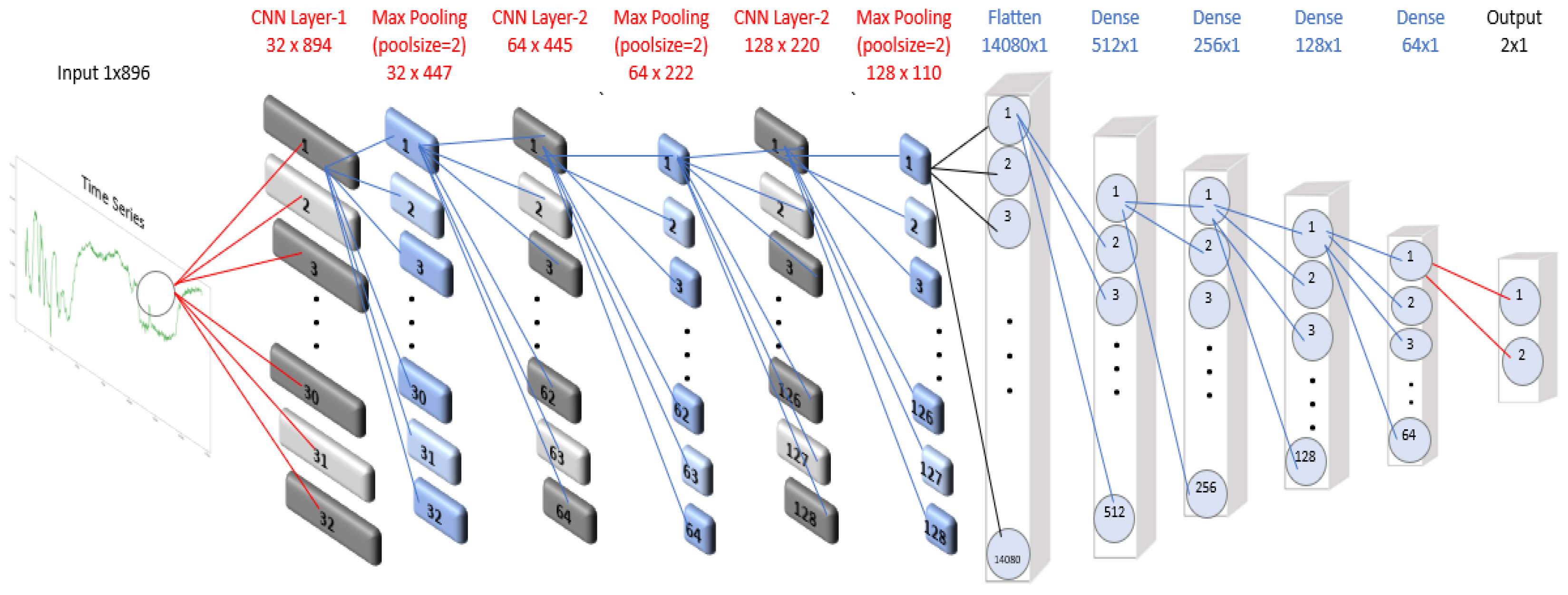
Figure 2.
Flow Chart of Research Process.
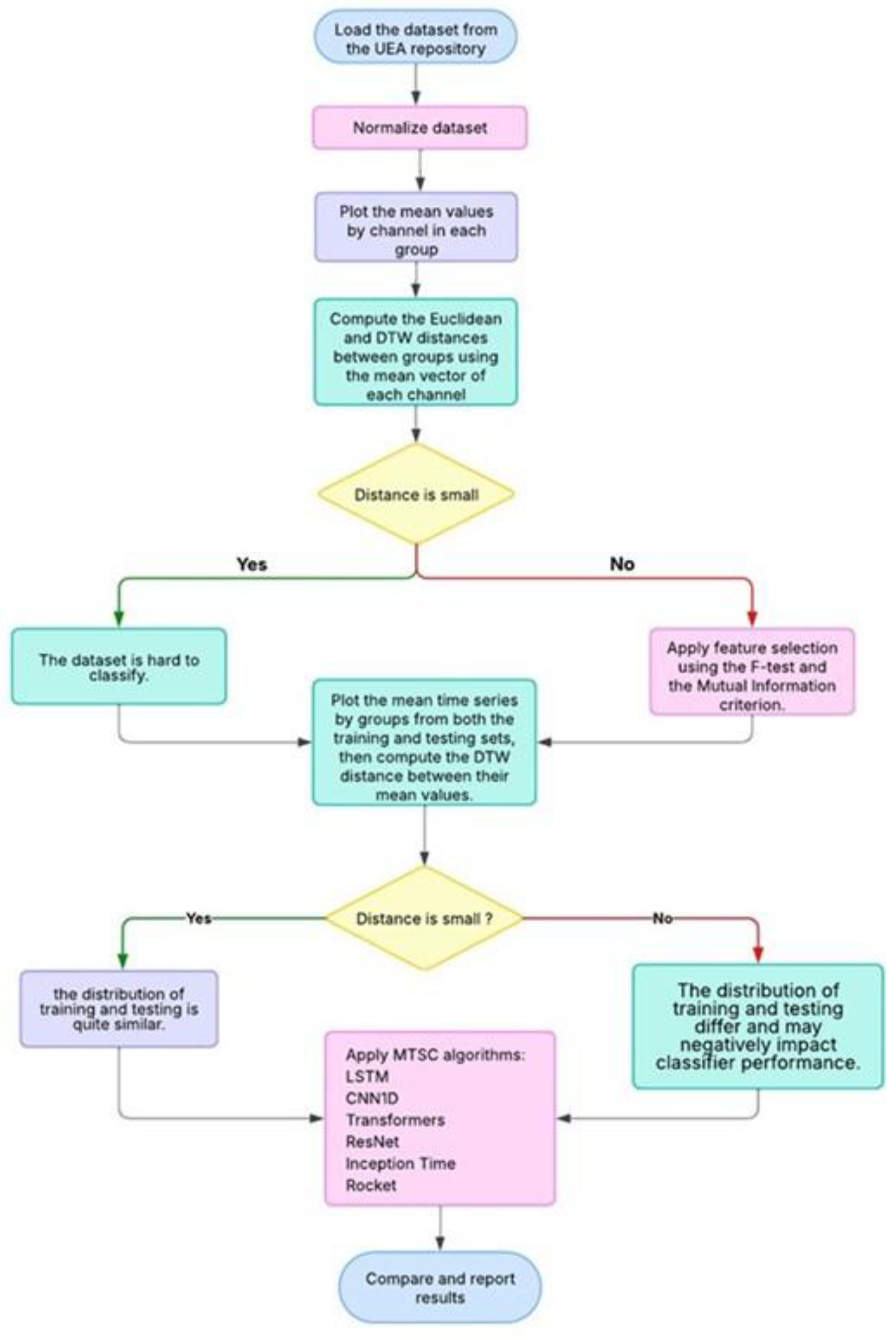
Figure 3.
Averaged time series by channel across the twelve groups in the CRI normalized training dataset. Channels are color-coded as follows: Ch1 = black, Ch2 = red, Ch3 = blue, Ch4 = cyan, Ch5 = magenta, and Ch6 = gray.
Figure 3.
Averaged time series by channel across the twelve groups in the CRI normalized training dataset. Channels are color-coded as follows: Ch1 = black, Ch2 = red, Ch3 = blue, Ch4 = cyan, Ch5 = magenta, and Ch6 = gray.
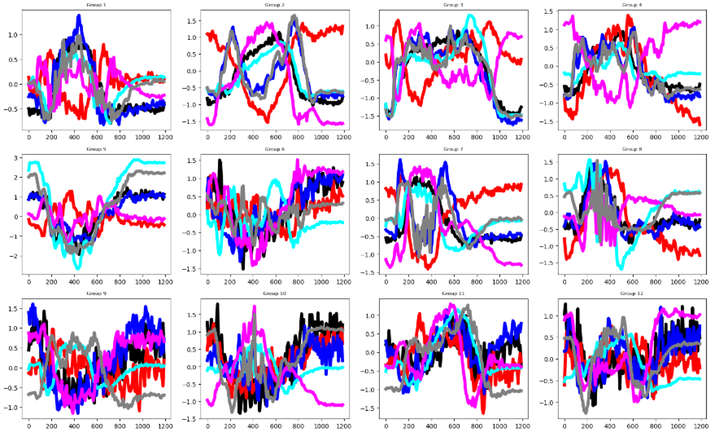
Figure 4.
Averaged time series across all groups for the CRI dataset: training set (top) and testing set (bottom).
Figure 4.
Averaged time series across all groups for the CRI dataset: training set (top) and testing set (bottom).
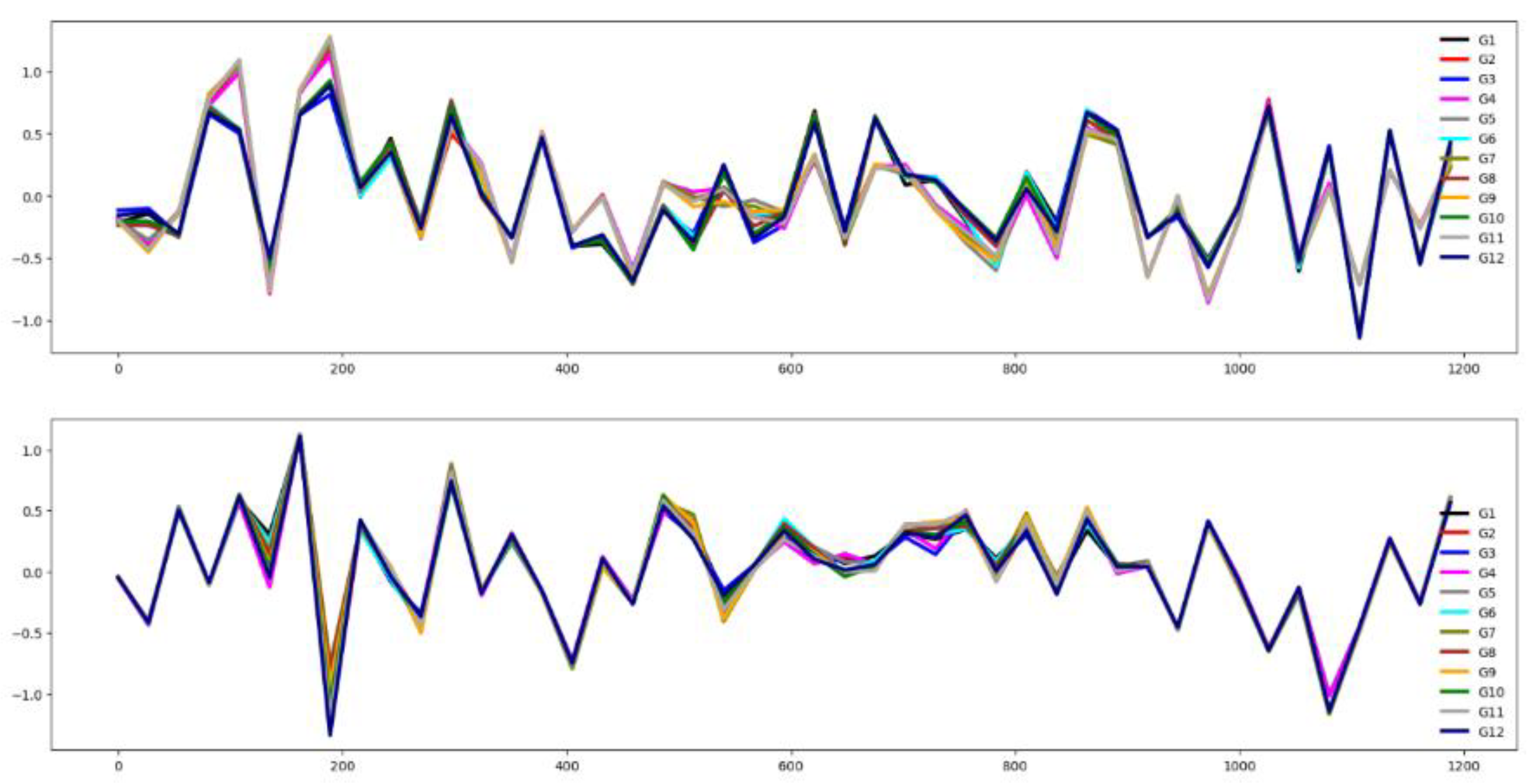
Figure 5.
Average time series by group across the six channels in the BM normalized training dataset. Groups are color-coded as follows: G1 = black, G2 = red, G3 = blue, and G4 = cyan.
Figure 5.
Average time series by group across the six channels in the BM normalized training dataset. Groups are color-coded as follows: G1 = black, G2 = red, G3 = blue, and G4 = cyan.
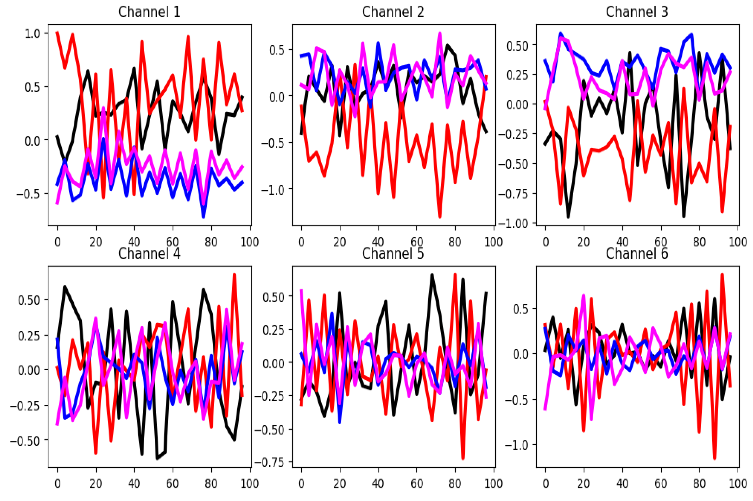
Figure 6.
Averaged time series for the BM dataset: training set (top) and testing set (bottom).
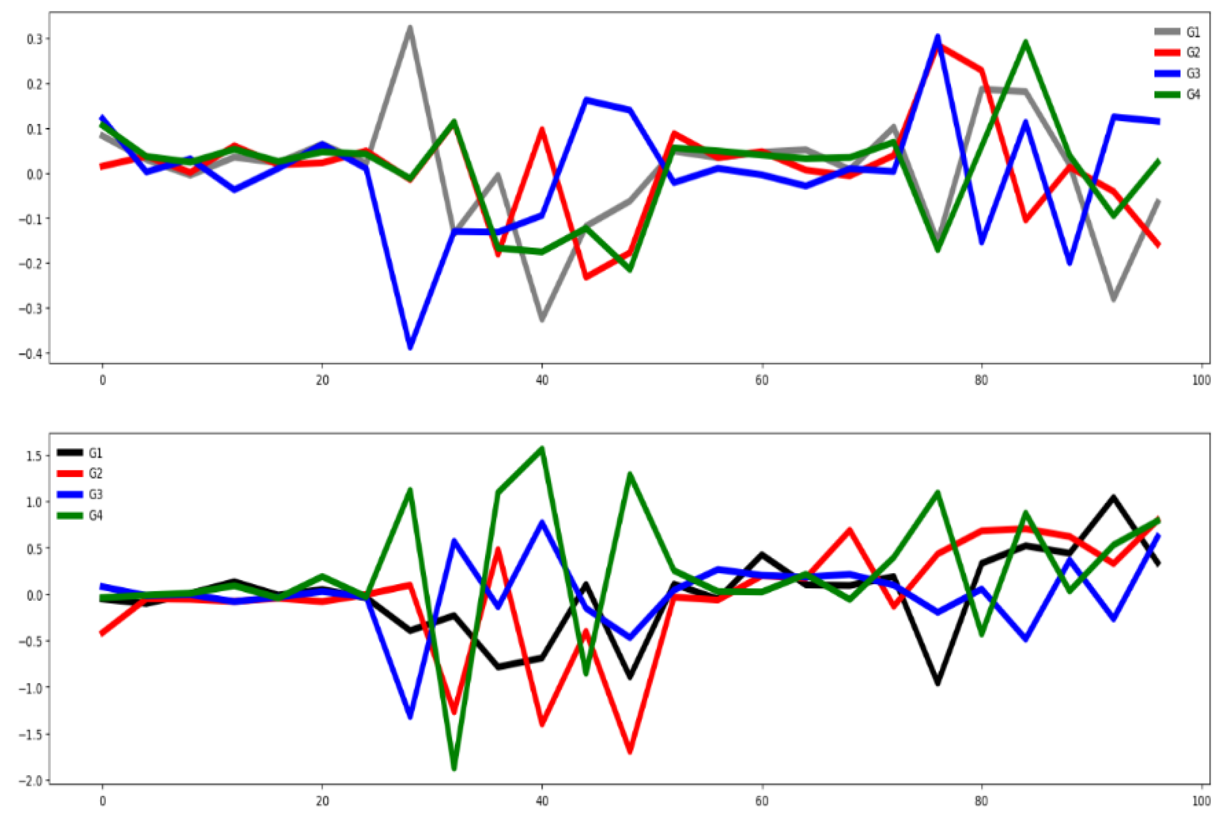
Figure 7.
Averaged time series by channel, segmented by group, for the EPI training dataset.
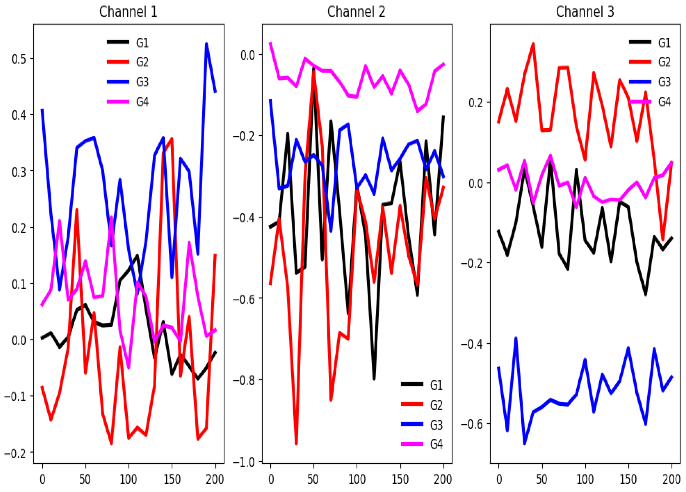
Figure 8.
Averaged time series segmented by group for the EPI training dataset (top) and testing dataset (bottom).
Figure 8.
Averaged time series segmented by group for the EPI training dataset (top) and testing dataset (bottom).

Figure 9.
Mean values of the channels, segmented by group (G1 = black, G2 = red, G3 = blue, G4 = cyan, G5 = magenta, G6 = orange), for the NATOPS training dataset.
Figure 9.
Mean values of the channels, segmented by group (G1 = black, G2 = red, G3 = blue, G4 = cyan, G5 = magenta, G6 = orange), for the NATOPS training dataset.
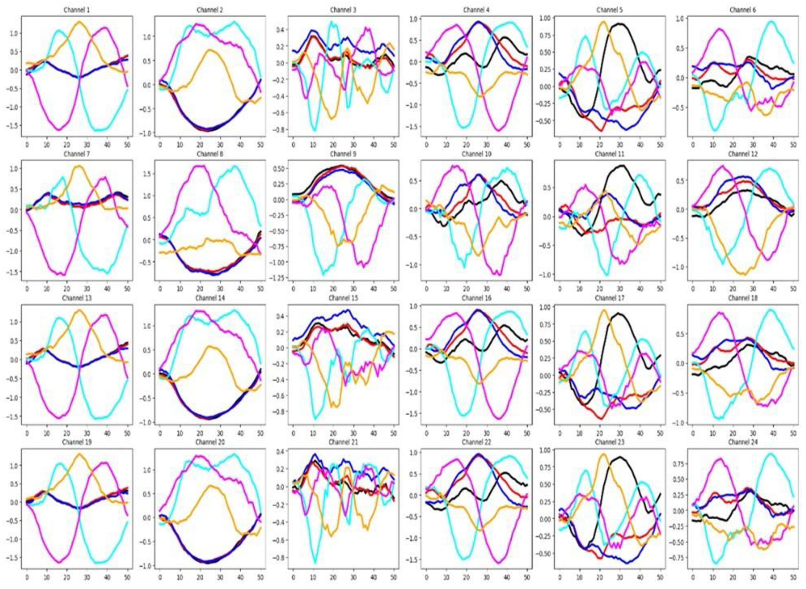
Figure 10.
Averaged time series segmented by group for the NATOPS training dataset (top) and testing dataset (bottom).
Figure 10.
Averaged time series segmented by group for the NATOPS training dataset (top) and testing dataset (bottom).
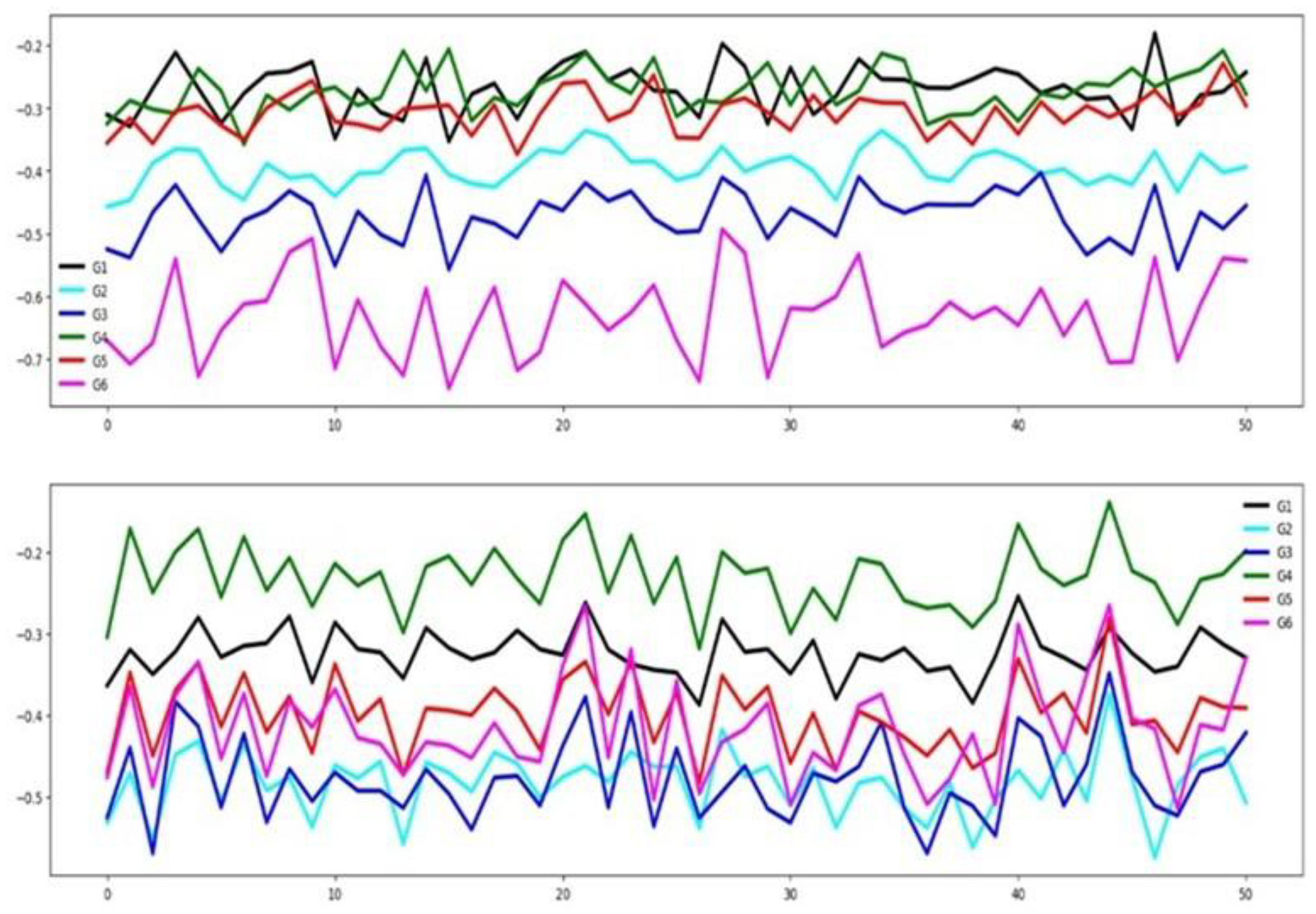
Figure 11.
Mean time series values for the 25 groups in each of the nine channels of the AWR training dataset.
Figure 11.
Mean time series values for the 25 groups in each of the nine channels of the AWR training dataset.
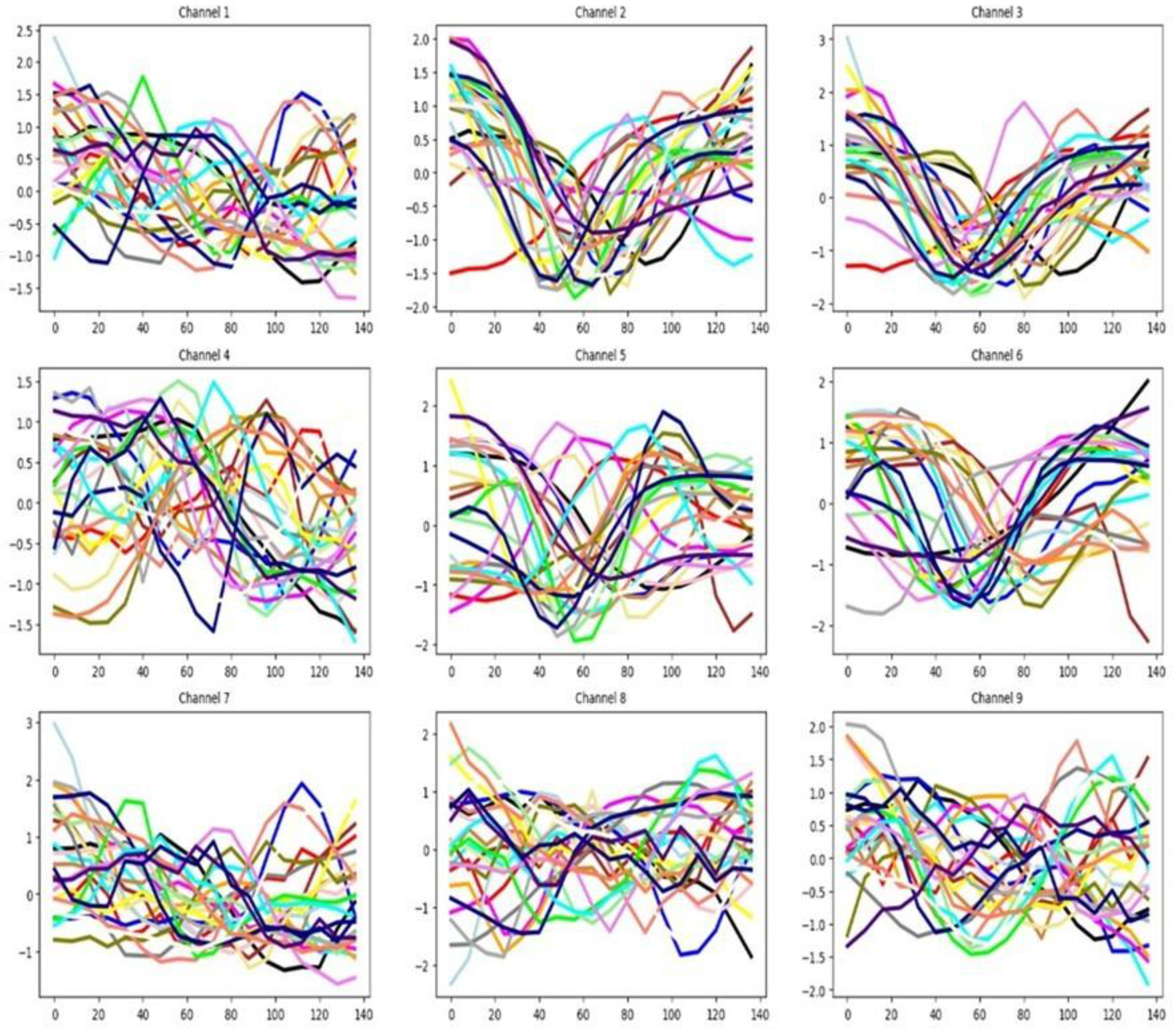
Figure 12.
Averaged time series values by group (G1 = black, G2 = red, G3 = blue, G4 = magenta) across the six channels of the RS training dataset.
Figure 12.
Averaged time series values by group (G1 = black, G2 = red, G3 = blue, G4 = magenta) across the six channels of the RS training dataset.
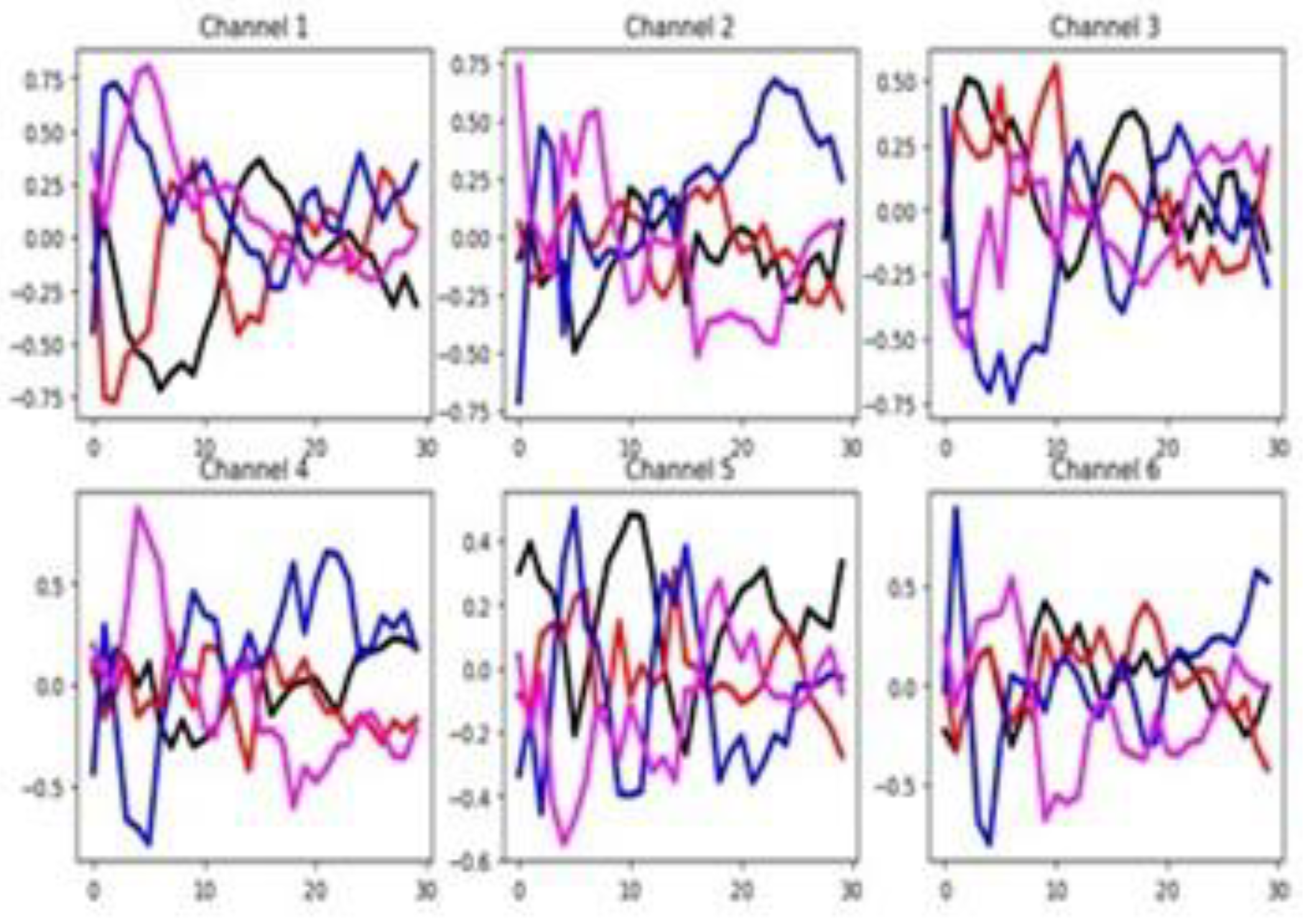
Figure 13.
Averaged time series across all groups for the RS dataset: training set (top) and testing set (bottom).
Figure 13.
Averaged time series across all groups for the RS dataset: training set (top) and testing set (bottom).
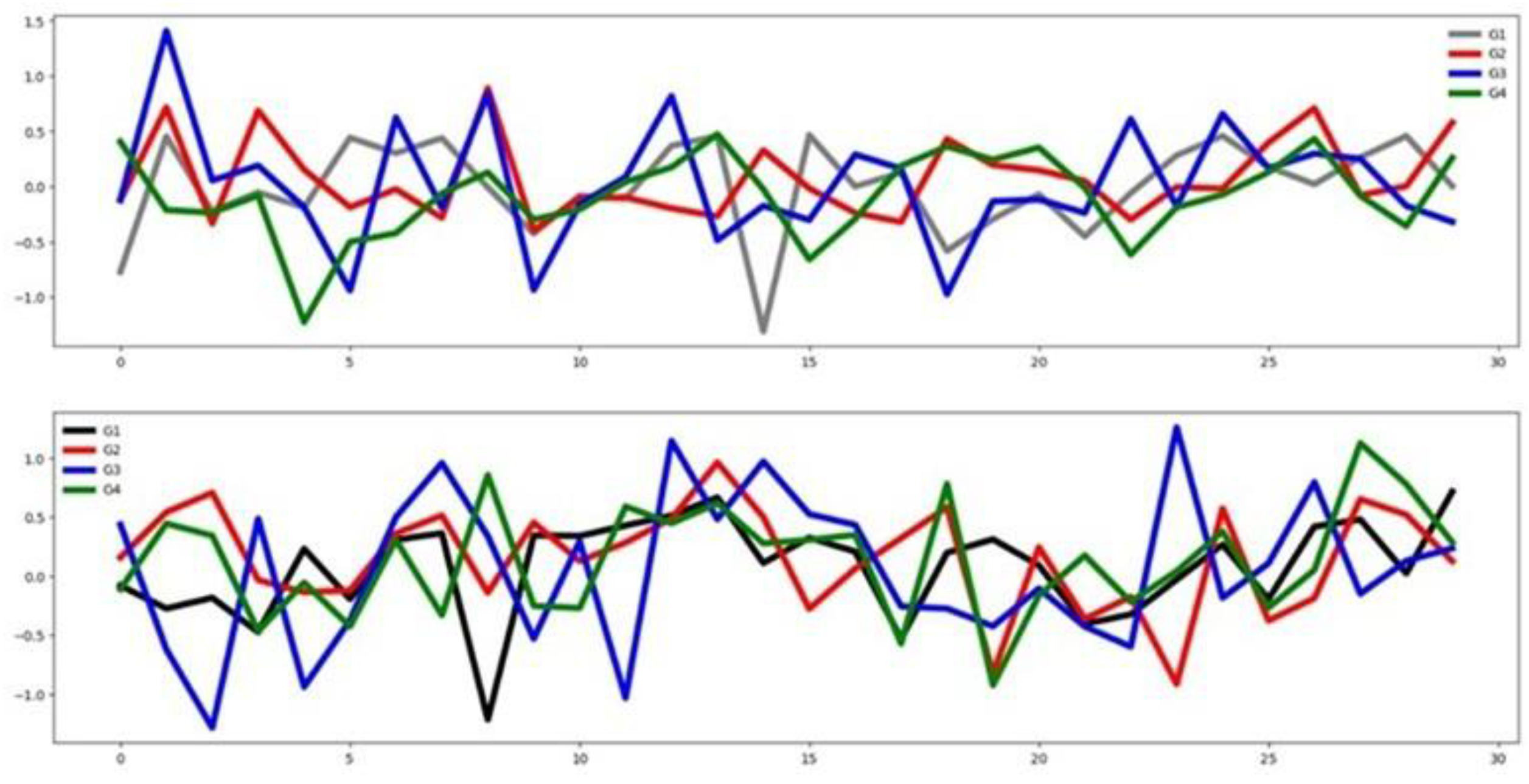
Figure 14.
Averaged time series of the seven groups (G1 = black, G2 = red, G3 = magenta, G4 = green, G5 = brown, G6 = yellow, G7 = blue) across the first 20 channels of the PEMS training dataset.
Figure 14.
Averaged time series of the seven groups (G1 = black, G2 = red, G3 = magenta, G4 = green, G5 = brown, G6 = yellow, G7 = blue) across the first 20 channels of the PEMS training dataset.
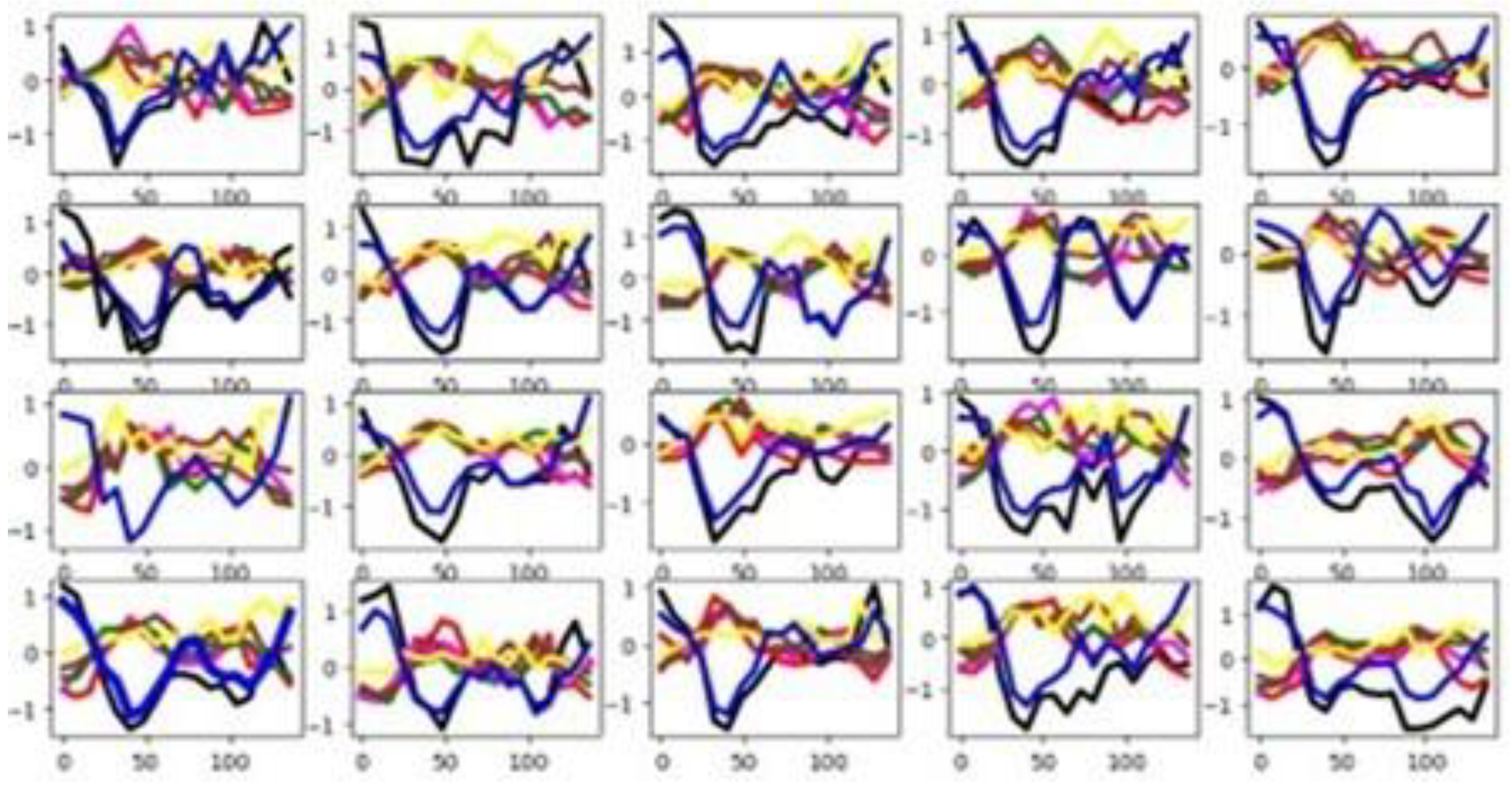
Figure 15.
Averaged time series by group (G1 = black, G2 = red) across the six channels of the SCP1 training dataset.
Figure 15.
Averaged time series by group (G1 = black, G2 = red) across the six channels of the SCP1 training dataset.
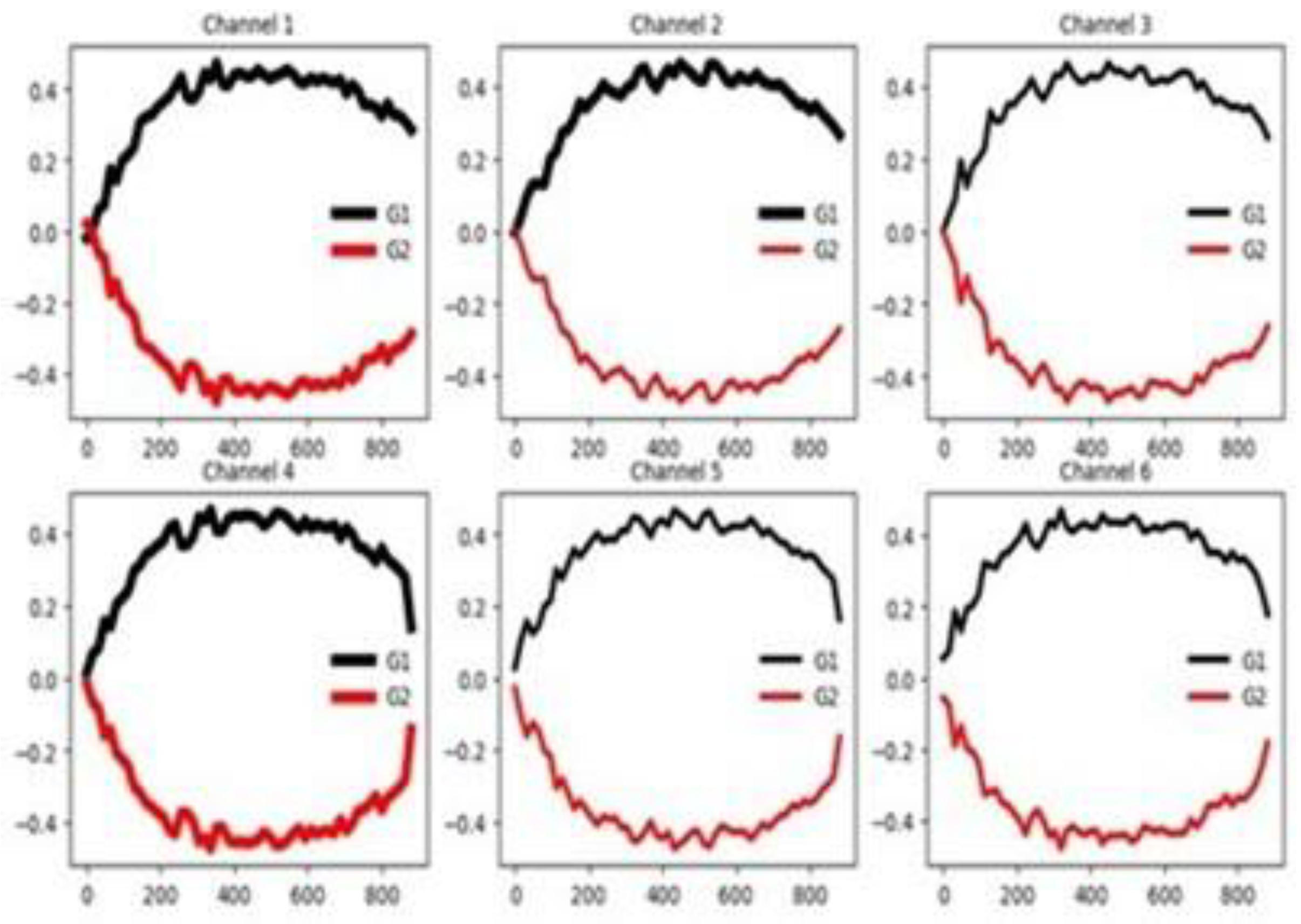
Figure 16.
Averaged time series segmented by group for the SCP1 training dataset (top) and testing dataset (bottom).
Figure 16.
Averaged time series segmented by group for the SCP1 training dataset (top) and testing dataset (bottom).
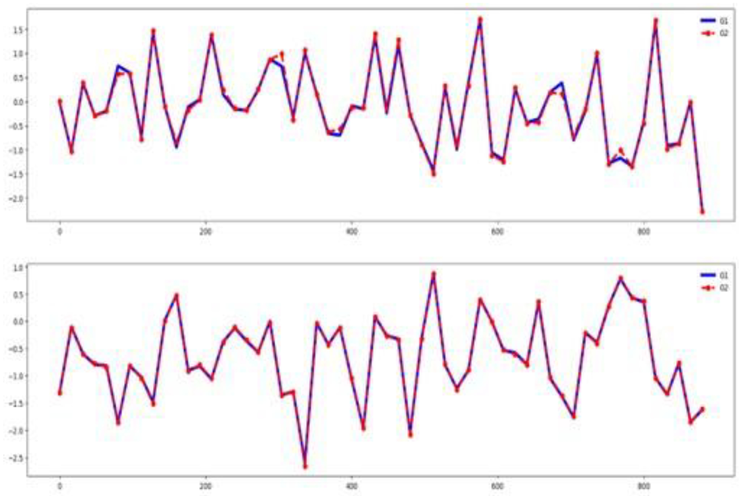
Figure 17.
Averaged time series by channel (Ch1 = black, Ch2 = red) across the fifteen groups of the LIB training dataset.
Figure 17.
Averaged time series by channel (Ch1 = black, Ch2 = red) across the fifteen groups of the LIB training dataset.

Figure 18.
Averaged time series by channel across both groups of the HB training dataset. Relevant channels are displayed in non-black colors.
Figure 18.
Averaged time series by channel across both groups of the HB training dataset. Relevant channels are displayed in non-black colors.
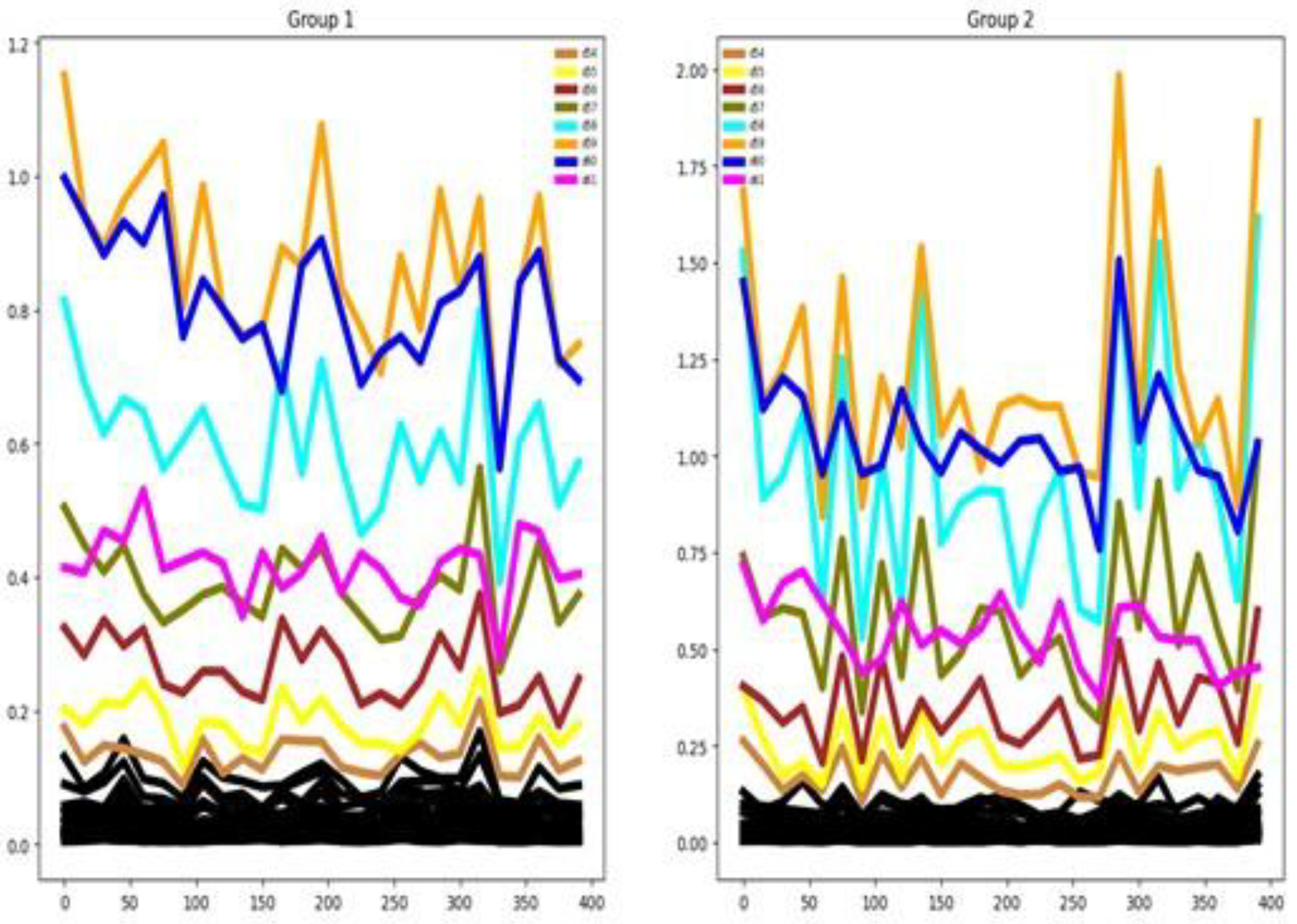
Figure 19.
Averaged time series segmented by group for the HB training dataset (top) and testing dataset (bottom).
Figure 19.
Averaged time series segmented by group for the HB training dataset (top) and testing dataset (bottom).
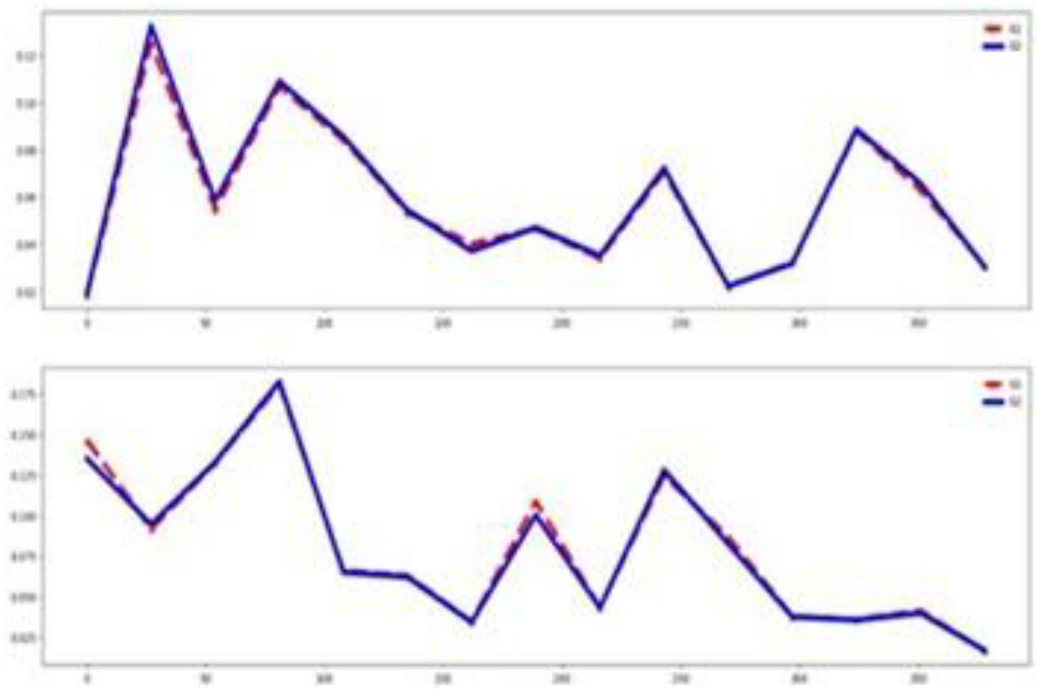
Figure 20.
Mean values of the first 20 channels, segmented by group (G1 = black, G2 = blue), for the FD training dataset.
Figure 20.
Mean values of the first 20 channels, segmented by group (G1 = black, G2 = blue), for the FD training dataset.
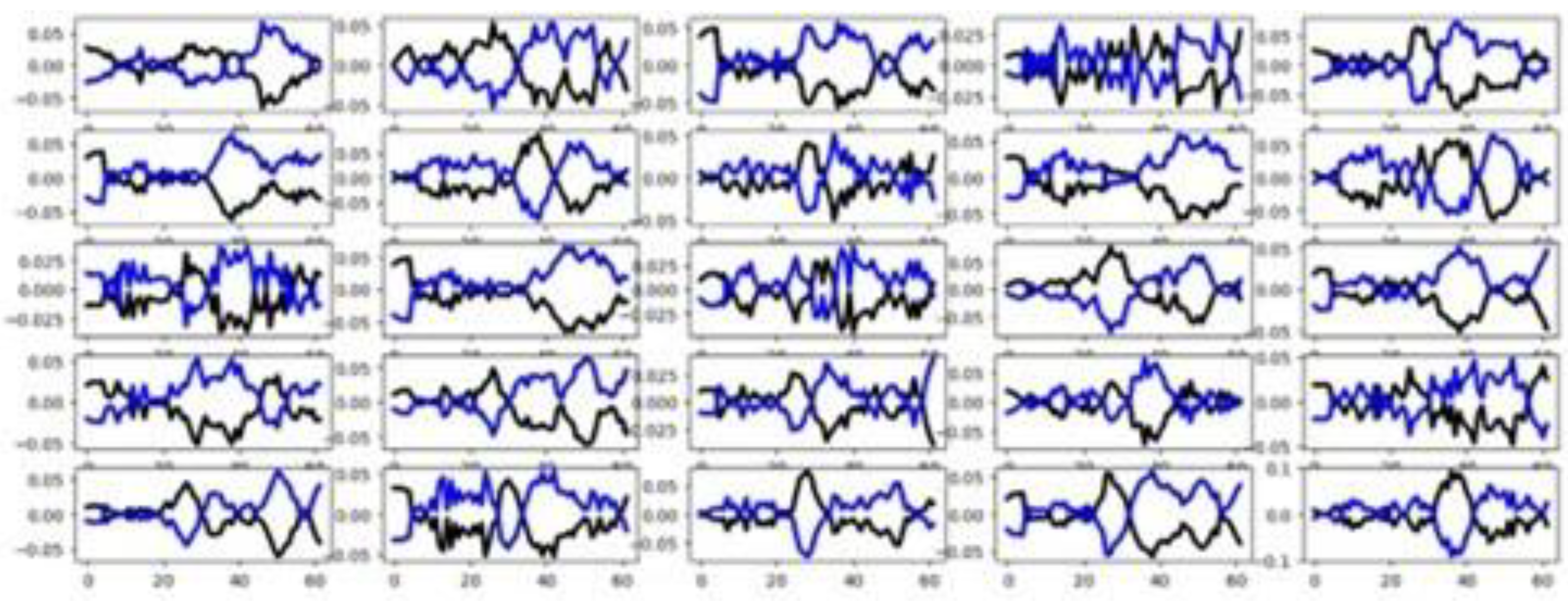
Figure 21.
Mean time series values in the first 20 channels, segmented by group (G1 = black, G2 = blue, G3 = red, G4 = cyan, G5 = magenta), for the normalized DDG training dataset. Very high peaks are observed in Groups 1 and 5.
Figure 21.
Mean time series values in the first 20 channels, segmented by group (G1 = black, G2 = blue, G3 = red, G4 = cyan, G5 = magenta), for the normalized DDG training dataset. Very high peaks are observed in Groups 1 and 5.

Figure 22.
Averaged time series by channel across groups for the SCP2 training dataset.
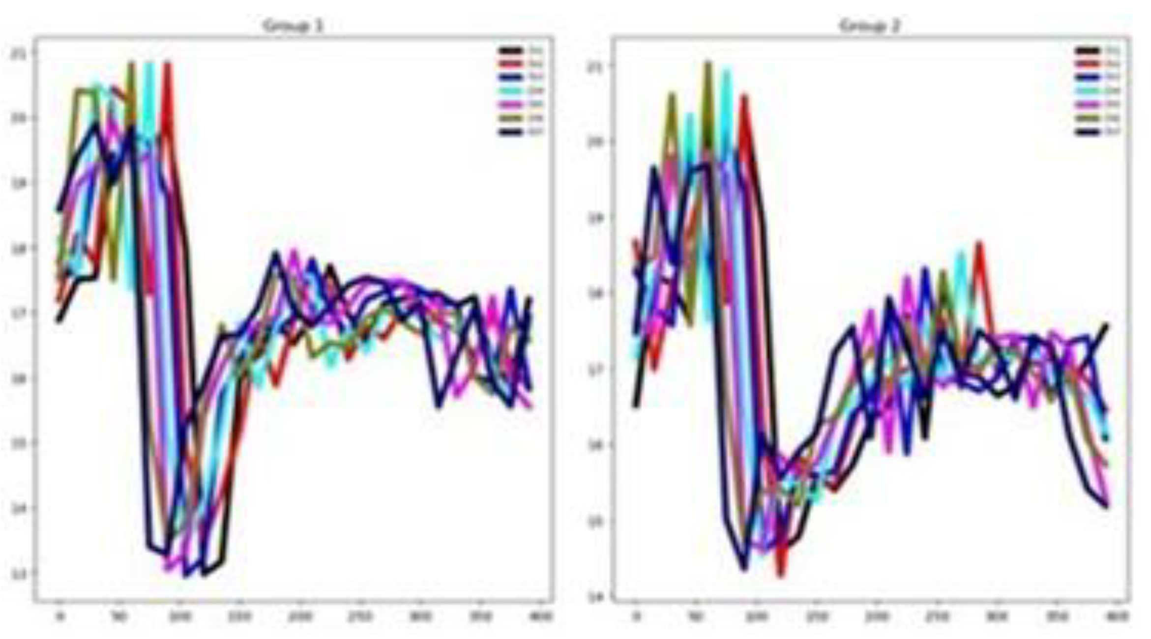
Figure 23.
Mean values by channel, segmented by group (G1 = black, G2 = red), for the FM training dataset.
Figure 23.
Mean values by channel, segmented by group (G1 = black, G2 = red), for the FM training dataset.
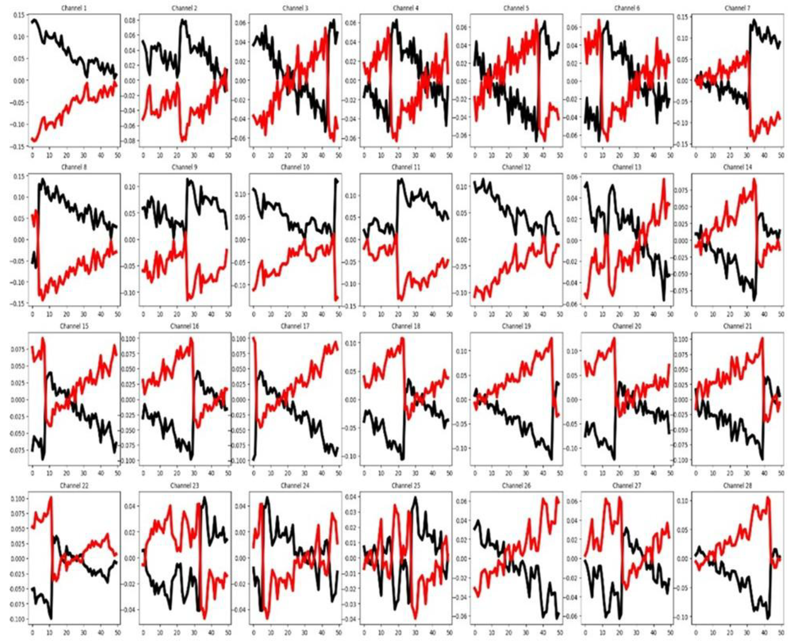
Figure 24.
Mean values by channel, segmented by group (G1 = black, G2 = red, G3 = blue, G4 = olive), for the HMD training dataset.
Figure 24.
Mean values by channel, segmented by group (G1 = black, G2 = red, G3 = blue, G4 = olive), for the HMD training dataset.
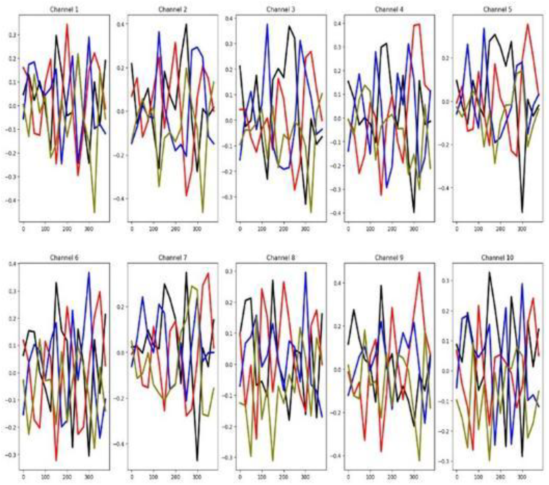
Figure 25.
Mean time series segmented by group for the HMD training dataset (top) and testing dataset (bottom).
Figure 25.
Mean time series segmented by group for the HMD training dataset (top) and testing dataset (bottom).
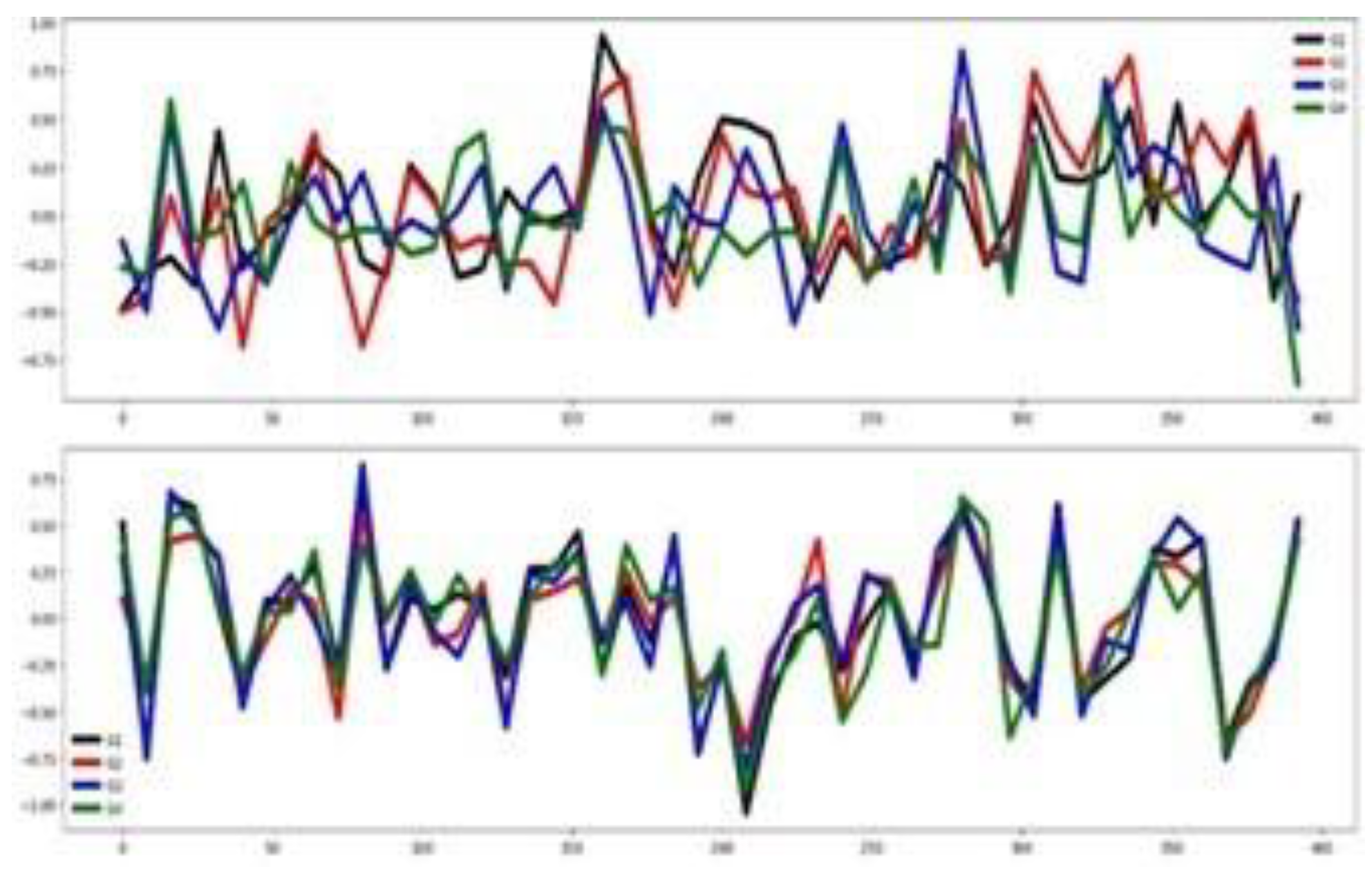
Figure 26.
Mean values by group (G1 = black, G2 = red, G3 = blue, G4 = magenta) across the three channels of the Ethanol Concentration training dataset.
Figure 26.
Mean values by group (G1 = black, G2 = red, G3 = blue, G4 = magenta) across the three channels of the Ethanol Concentration training dataset.
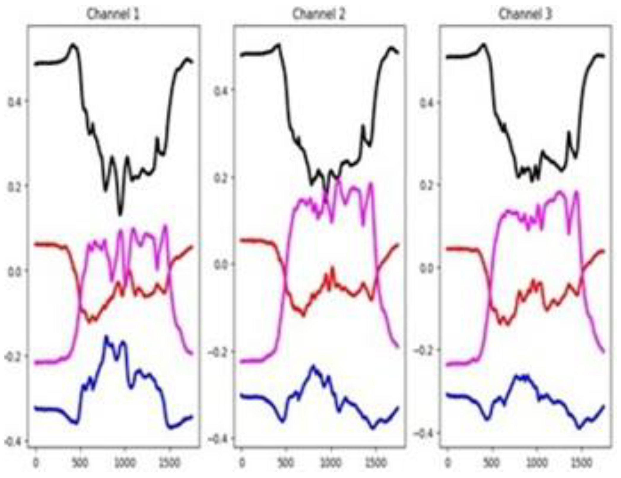
Figure 27.
Mean time series across groups for the EC training dataset (top) and EC testing dataset (bottom).
Figure 27.
Mean time series across groups for the EC training dataset (top) and EC testing dataset (bottom).


Table 1.
Summary of the datasets considered in the experiments.
| Dataset | Train | Test |
Channels (Ch) |
Length | Groups | Train*Ch | Train*Ch/L | Acc. Default % |
| CRI [23] | 108 | 72 | 6 | 1197 | 12 | 648 | 0.54 | 8.33 |
| BM [2] | 40 | 40 | 6 | 100 | 4 | 240 | 2.40 | 25.00 |
| EPI [24] | 137 | 138 | 3 | 206 | 4 | 411 | 1.99 | 26.80 |
| NATOPS [25] | 180 | 180 | 24 | 51 | 6 | 4320 | 84.70 | 26.81 |
| AWR [10] | 275 | 300 | 9 | 144 | 25 | 2475 | 17.18 | 4.00 |
| RS [2] | 151 | 152 | 6 | 30 | 4 | 906 | 30.20 | 28.30 |
| PEMS [26] | 267 | 173 | 963 | 144 | 7 | 257121 | 1786.00 | 17.34 |
| SCP1 [27] | 268 | 293 | 6 | 896 | 2 | 1608 | 1.79 | 50.20 |
| LIB [28] | 180 | 180 | 2 | 45 | 15 | 360 | 8.00 | 6.70 |
| HB [29] | 204 | 205 | 61 | 405 | 2 | 12444 | 30.70 | 72.19 |
| FD [30] | 5890 | 3524 | 144 | 62 | 2 | 848160 | 13680.00 | 50.00 |
| DDG [31] | 50 | 50 | 1345 | 270 | 5 | 67250 | 249.00 | 20.00 |
| SCP2 [27] | 200 | 180 | 7 | 1152 | 2 | 1400 | 1.22 | 50.00 |
| FM [32] | 316 | 100 | 28 | 50 | 2 | 8848 | 177.00 | 51.00 |
| HMD [30] | 160 | 74 | 10 | 400 | 4 | 1600 | 4.00 | 40.54 |
| EC [33] | 261 | 263 | 3 | 1751 | 4 | 783 | 0.44 | 25.09 |
Table 2.
Accuracy of deep learning classifiers evaluated in the testing set.
| Dataset | LSTM | CNN-1D | Transformer | ResNet | Inception Time | Rocket | ||||||
| CRI | 93.20 | ±4.96 | 94.10 | ±2.18 | 69.00 | ±7.15 | 98.84 | ±0.57 | 98.41 | ±0.96 | 100.00 | ±0.00 |
| BM | 97.00 | ±1.82 | 100.00 | ±0.00 | 82.85 | ±6.98 | 97.00 | ±6.70 | 55.20 | ± 2.82 | 100.00 | ±0.00 |
| EPI | 82.53 | ±1.79 | 83.48 | ±1.44 | 76.45 | ±3.33 | 94.05 | ±4.30 | 93.62 | ±5.11 | 99.20 | ±0.79 |
| NATOPS | 83.99 | ±1.69 | 91.67 | ±1.94 | 77.07 | ±5.09 | 92.88 | ±2.68 | 94.27 | ±1.14 | 88.32 | ±0.64 |
| AWR | 87.92 | ±2.09 | 92.93 | ±1.26 | 48.78 | ±3.19 | 93.36 | ±5.70 | 97.56 | ±2.22 | 99.29 | ±0.18 |
| RS | 75.80 | ±1.98 | 82.00 | ±2.89 | 66.00 | ±4.26 | 88.68 | ±2.0 | 88.28 | ±1.35 | 91.17 | ±0.59 |
| PEMS | 89.70 | ±2.22 | 88.55 | ±4.27 | 78.09 | ±2.78 | 73.80 | ±6.95 | 73.86 | ±6.21 | 81.26 | ±1.44 |
| SCP1 | 77.74 | ±1.51 | 85.60 | ±2.11 | 75.63 | ±2.91 | 73.03 | ±6.40 | 76.79 | ±8.80 | 84.88 | ±1.02 |
| LIB | 74.60 | ±6.27 | 79.50 | ±2.27 | 54.50 | ±3.17 | 81.66 | ±10.51 | 87.44 | ±0.63 | 90.55 | ±0.39 |
| HB | 71.70 | ±1.21 | 73.56 | ±1.30 | 73.72 | ±2.13 | 57.56 | ±9.77 | 67.36 | ±9.45 | 74.48 | ±0.94 |
| FD | 63.62 | ±0.79 | 61.14 | ±0.46 | 61.38 | ±1.14 | 55.26 | ±1.14 | 65.92 | ±0.94 | 58.67 | ±0.55 |
| DDG | 51.80 | ±5.62 | 62.00 | ±4.42 | 42.60 | ±6.80 | 59.80 | ±4.46 | 61.20 | ±2.35 | 49.40 | ±3.27 |
| SCP2 | 53.93 | ±2.67 | 53.60 | ±2.01 | 51.94 | ±2.80 | 51.10 | ±1.75 | 52.77 | ±2.79 | 55.16 | ±2.06 |
| FM | 51.79 | ±3.18 | 51.80 | ±2.09 | 50.40 | ±3.02 | 53.60 | ±4.14 | 55.20 | ± 2.82 | 55.10 | ±1.28 |
| HMD | 38.11 | ±8.14 | 52.30 | ±2.40 | 36.10 | ±4.35 | 30.40 | ±3.89 | 40.80 | ±1.89 | 50.89 | ±3.57 |
| EC | 26.92 | ±1.90 | 41.50 | ±10.36 | 27.97 | ±2.35 | 27.63 | ±2.18 | 28.09 | ±2.79 | 40.83 | ±1.88 |
Table 3.
Summary of several measures computed for each dataset.
| Dataset | % of relevant channels | % of relevant Features | Min Eucl. Dist_group | Min DTW Dist_group | Min DTW Dist_group |
Mean DTW Dist Train_test |
|
| F-test | MI | ||||||
| CRI | 100.00 | 2.59 | 7.60 | 1.43 | 1.40 | 1.40 | 7.90 |
| BM | 50.00 | 9.00 | 9.00 | 1.51 | 0.92 | 0.92 | 0.76 |
| EPI | 33.33 | 0.48 | 7.28 | 1.60 | 1.46 | 1.46 | 3.12 |
| NATOPS | 70.83 | 5.88 | 17.64 | 0.37 | 0.36 | 0.36 | 0.37 |
| AWR | 100.00 | 0.69 | 11.81 | 0.66 | 0.52 | 0.52 | 0.57 |
| RS | 66.67 | 3.33 | 46.66 | 0.44 | 0.31 | 0.31 | 0.30 |
| PEMS | 33.02 | 4.86 | 14.58 | 0.05 | 0.05 | 0.05 | 1.45 |
| SCP1 | 50.00 | 0.55 | 1.34 | 2.47 | 2.45 | 2.45 | 22.15 |
| LIB | 100.00 | 20.00 | 37.77 | 1.59 | 1.37 | 1.37 | 3.51 |
| HB | 14.75 | 0.49 | 11.85 | 0.37 | 0.37 | 0.37 | 12.92 |
| FD | 8.33 | 14.52 | 19.35 | 0.02 | 0.01 | 0.01 | 0.05 |
| DDG | 28.77 | 1.11 | 10.00 | 0.20 | 0.20 | 0.20 | 8.76 |
| SCP2 | 71.40 | 0.17 | 0.00 | 2.19 | 2.18 | 2.18 | 18.14 |
| FM | 21.42 | 12.00 | 14.00 | 0.06 | 0.06 | 0.06 | 3.06 |
| HMD | 20.00 | 8.25 | 13.00 | 4.34 | 3.75 | 3.75 | 5.05 |
| EC | 100.00 | 2.85 | 21.01 | 3.60 | 3.58 | 3.58 | 21.91 |
Disclaimer/Publisher’s Note: The statements, opinions and data contained in all publications are solely those of the individual author(s) and contributor(s) and not of MDPI and/or the editor(s). MDPI and/or the editor(s) disclaim responsibility for any injury to people or property resulting from any ideas, methods, instructions or products referred to in the content. |
© 2025 by the authors. Licensee MDPI, Basel, Switzerland. This article is an open access article distributed under the terms and conditions of the Creative Commons Attribution (CC BY) license (http://creativecommons.org/licenses/by/4.0/).
Copyright: This open access article is published under a Creative Commons CC BY 4.0 license, which permit the free download, distribution, and reuse, provided that the author and preprint are cited in any reuse.


