
Submitted:
14 March 2025
Posted:
17 March 2025
You are already at the latest version
Abstract
Raw biomass (low bulk density) is converted to pellets (high bulk density) in several pellet depots. The distribution of these depots across the production area has impact of the total truck operating hours (raw biomass hauling to a depot + pellet hauling from the depot to the biorefinery) required to delivery feedstock for annual operation of the biorefinery. This study examines the distribution of depots across five production areas. The number of depots were 1, 2, and 4 depots per production area for a total of 5, 10, and 20 depots. Increasing from 5 to 10 reduced raw biomass hauling hours by 14% and increasing from 5 to 20 reduced these hours by 30%. Total hours (raw + pellets) were reduced less than 1% from 5 to 10 and about 11% from 5 to 20.
Keywords:
biomass
; logistics
; truck transport
; depot distribution
; switchgrass
1. Introduction
The Southeastern USA has the potential for a significant biorefinery industry. One challenge is the low feedstock density, defined as the Mg of feedstock production potential per square km within a given radius of the proposed biorefinery location. As the radius of the feedstock production area for the biorefinery increases, the per-Mg feedstock delivery cost increases, because the average cycle time for the total loads increases. Thus, truck productivity (Mg/d) decreases, and truck cost (USD/Mg) increases.
A round-bale system is the best option for the Piedmont, a 166-county physiographic region across five Southeastern states. Work has been done to eliminate single-bale handling for loading and unloading, an important operational parameter in the logistics system [1,2,3].
Certain biorefinery designs require high capacity to achieve the necessary economy-of-scale. It is often not economical to meet the feedstock demand by hauling low-bulk-density biomass from the surrounding production area. Consequently, the US DOE introduced a concept where a network of depots producing an intermediate feedstock (i.e., material at higher bulk density and higher energy density) would supply a biorefinery [4,5]. Others have continued the study of the influence of depot distribution on average delivered feedstock cost [6,7,8].
As a specific example applicable to this study, a load of 40 round bales is 16 Mg and a load of pellets is 34 Mg. Cost to operate the truck (USD/h) is approximately the same (small difference in fuel consumption) for both loads. The question then emerges, what impact does the distribution of pellet depots have on the total truck operating hours (raw biomass hauling + pellet hauling) to deliver biomass to a biorefinery for annual operation?
A modular pellet plant design has been developed by The PelletMaster Modular Pellet Plant [9], and this technology provides an opportunity to consider smaller-scale pellet depots. Now it is possible to consider a larger number of widely dispersed depots, as opposed to a smaller number of more centrally located large capacity depots.
An ultimate implementation of the concept might envision that each farmgate contract holder would own their own pellet plant. This would mean that farmgate contracts are limited to those who can get the capitalization required to purchase and install the modular plant. Also, there are the requirements for the required expertise to operate the plant, and the requirement that this system of depots operate to provide a year-round supply of pellets. All three of these issues, capitalization, operational expertise, and continuous year-round supply to biorefinery, argue against a “farm-level” implementation of the concept, and in favor of the “community-level” implementation, proposed for this study.
There or over 200,000 trucking companies in the US, thus, truck cost (USD/h) is well defined for the heavy truck industry. A business plan is needed which will minimize the truck operating hours to deliver feedstock for year-round operation of the biorefinery. The total truck cost includes the cost to deliver the raw biomass to a pellet depot, plus the subsequent cost to deliver pellets to the biorefinery.
A single depot at the center of a 48-km radius production area gives an increased number of truck operating hours for the delivery of raw biomass. Consequently, a wider distribution of depots reduces the raw biomass trucking hours, but it may increase the operating hours to deliver the pellets. This study was done to quantify comparison of the total truck operating hours, raw biomass hauling + pellet hauling, for several depot distributions across five production areas, each having a different feedstock density.
Total truck operating hours were calculated for three depot distributions within a 48-km radius production area: (1) a single depot at the center of the area pelleting 100% of the stored biomass, (2) two depots, each pelleting approximately 50% of the stored biomass, and (3) four depots, each pelleting approximately 25% of the stored biomass.
2. Methodology
2.1. Study Area
As defined for two previous depot studies [10,11], three zones were selected from the South-Central Virginia Piedmont (VA5, VA6, VA7) and two zones were selected from the North-Central North Carolina Piedmont (NC2, NC3). Each of these zones, hereafter referred to as production areas, were assigned the same three depot distributions, defined as Depot-1, Depot-2, and Depot-4. The total depots for the five production areas supplying the biorefinery were then 5 for Depot-1, 10 for Depot-2, and 20 for Depot-4.
2.2. Criteria for Locating Depots and Biorefinery Site
Many constraints have been used in the literature to define the feedstock supply radius, i.e., the distance between the production fields and a biorefinery. Gustafson et al. [12] used a 161-km (100-mi) radius to define the supply of wheat straw and corn stover to a potential biorefinery. Holder et al. [13] assumed an 80-km (50-mi) radius for corn feedstock biorefineries. Lynch and Satrio [14] used a 97-km (60-mi) radius to define the distance between switchgrass fields and a theoretical biorefinery. For this study, a biorefinery location was chosen near South Boston, VA with convenient access to a four-lane highway and an existing rail siding. The radius encompassing the total depots for each of the three distributions was 97 km. Only the 5-depot distribution is shown in Figure 1.
2.3. Potential Raw Biomass Production Available for the Five Depots
Potential switchgrass feedstock production was estimated from current land cover within a 48-km (30-mi) radius, the same production area used for previous studies [10,11], identified as the “Gretna” database. These buffered areas were then clipped to the multi-county production zones, so the production area for each depot did not overlap. All spatial analyses and geoprocessing were performed using ArcGIS 10.6 (Redlands, CA, USA).
The herbaceous feedstock was assumed to be switchgrass (Panicum virgatum L.), which is a perennial warm-season grass that has been shown to have significant potential as feedstock for a biorefinery. The switchgrass feedstock was assumed to be harvested from fields and stored in satellite storage locations ( SSLs) in round bales with an average moisture content of 15%. An average switchgrass yield of 6.7 Mg/ha was assumed over all five production areas [15]. The total annual production for the nth production area is
Qn = the total annual production (Mg) for nth production area
(n = 1 VA5, n = 2 VA6, n = 3 VA7, n = 4 NC2, and n = 5 NC3)
An = the total feedstock production area (ha) within a 48-km radius
yld = the average switchgrass yield across the entire production area (Mg/ha).
The land cover area, ranging from 30,077 to 63,572 ha, was multiplied by the percent expected to be attracted into switchgrass production (40%) and then multiplied by the assumed average switchgrass yield (6.7 Mg/ha) to estimate the annual production for each production area (Table 1). The potential annual production ranged from 80,607 Mg (VA5) to 170,372 Mg (VA6), resulting in a total raw biomass production of 555,393 Mg, which could potentially be delivered annually to supply a biorefinery.
2.4. Procedure for Analysis of Satellite Storage Location (SSL) Databases
The database for each production area was assigned the same SSL distribution analyzed for the Gretna database. The road distance to each SSL, relative to the proposed centrally located depot location (i.e., the center of the 48-km radius), was defined in the Gretna database, and this same matrix was used for all five databases in this study. A feedstock density multiplication factor (Fi) was defined as:
where:
Qn= the total annual production (Mg) for the nth production area (Table 1);
Qb= the total annual production defined for the Gretna database (152,526 Mg).
The only difference among the five production areas was the quantity of biomass harvested and stored in each SSL, as defined by the feedstock density factor [Eq. (2)].
The same load-out methodology described by Resop and Cundiff [10] and Resop et al. [11] was used for each of the five production area databases in this study. As done for the previous studies, a truckload was two 20-bale handling units per truck [1]. Modern balers can produce 5 x 4 round bales (1.5 m dia. x 1.2 m long) of switchgrass that weigh about 0.4 Mg (15% MC), resulting in 16 Mg of raw biomass per 40-bale truckload.
2.5. Databases for Hauling Analyses
There were three analyses done. The Depot-1 analysis was done for a single depot located at the center of the 48-km radius production area. The Depot-2 analysis was done for two depots in the production area. To locate these depots, the production area was divided so that approximately 50% of the total stored biomass was alocated to each depot. [These areas are defined as L1 and L2 (Figure 2).] The two depots were positioned so that the mass-distance parameter, within each subarea, was approximately equal for both.
The Depot-4 analysis was done for four depots in the production area. The area was divided so that approximately 25% of the total stored biomass was alocated to each depot. [These zones are defined as L1, L2, L3, and L4 (Figure 3).] As with the Depot-2 analysis, the depots were positioned so that the mass-distance parameter was approximately equal for all four.
There are a total of 10 depots, two depots for each of the five production areas, that supply the biorefinery for the Depot-2 analysis. . There are a total of 20 depots, four for each of the five production areas, that supply the biorefinery for the Depot-4 analysis.
A matrix was created with the road distance from each SSL to its assigned depot. This matrix defines the haul distance for raw biomass to that depot.
The number of load-out operations for each database were the same as described by Resop and Cundiff [10] and Resop et al. [11] (Table 2). Each loadout moved through the same sequence of SSLs as in the previous studies; the only difference was the truck scheduling. Rather than delivering to a single centrally located depot, the trucks hauled to their new depot assignment (Figure 2 and Figure 3).
The capacity of the pellet depots was calculated using the following parameters: average moisture content of raw biomass = 15% (wb); ratio of raw biomass to pellets = 1.1 dry matter basis; moisture content of shipped pellets = 6% (wb). This gave a conversion factor of 0.822. Depots are expected to operate 7 d/wk for 48 wk/y = 336 d/y. The resulting capacity (Mg pellets/d) is given in Table 3, Table 4 and Table 5 for the Depot-1, Depot-2, and Depot-4 analyses, respectively. The smallest depot was 47.7 Mg/d (VA5-L4) and the largest was 417.9 Mg/d (VA6-Central), giving a 10:1 ratio in depot capacity across the entire study.
The highway distance to haul pellets from each of the 5 depots in the Depot-1 analysis is shown in Figure 4 and the distances are given in Table 6. The highway distance for the 10 depots in the Depot-2 analysis is shown in Figure 5, and the distances are given in Table 7. In like manner, the highway distance for each of the 20 depots in the Depot-4 analysis is given in Figure 6, and the distances are given in Table 8.
2.6. Truck Operating Hours to Haul Raw Biomass
Truck operating hours for hauling raw biomass were determined using the following procedure. Ideal truck cycle time was calculated based on the following assumptions:
- Load time was defined to be Lt =15 min.
- Unload time was defined to be Ut=20 min.
- Travel speed over rural roads averages 70 km/h.
The ideal truck cycle time (i.e., assuming no delays) for hauls from the jth SSL located a distance hdj from the assigned depot was computed as:
A multiplier of 1.4 was used to obtain truck achieved average cycle time (Taj), defined as
This multiplier accounted for delays in loading (e.g., waiting at SSL) and unloading (e.g., waiting at the depot receiving facility), plus delays due to traffic. This is an optomistic achieved cycle time, but it does define a "baseline" truck fleet size.
Number of loads was based on a load of 40 bales equal to 16 Mg. This then defines the number of loads (nlj) hauled from the jth SSL. (No partial loads are considered. Typically there will be some remaining bales, and there is potential for a mobile pelleting unit to travel from SSL to SSL to process these bales into pellets. This option is not explored here.) Total truck operating hours to haul all loads from the jth SSL is now given by
Total truck operating hours for the three analyses was calculated as follows. The operating hours were first summed for all SSLs assigned to a given depot. This calculation is straight forward for the Depot-1 simulation because all SSLs within a given production area (all 199) supply biomass to one centrally located depot. This total is designated Tohn for the nth production area.
To obtain the total for all five production areas
For the Depot-2 simulation, the SSLs assigned to the two depots are not sequential. Remember, the decision was made to use the same load-out procedure (same sequence of SSL load-outs) for all three analyses. Thus, a matrix was created to list the SSL numbers in the needed sequence. Then, the sumation was done for this number of SSLs to obtain TohL1n for the L1 depot and TohL2n for the L2 depot. The total for the Depot -2 distribution is
The same procedure was used for the Depot-4 simulation. The Toh for the SSLs assigned to a given depot in the nth production area were summed to obtain TohL1n, TohL2n, TohL3n, and TohL4n for the L1, L2, L3, and L4 depots, respectively. The total for the Depot-4 distribution is
2.7. Truck Travel to Haul Raw Biomass
Total haul distance to haul all loads of raw biomass from the jth SSL is given by
The same summation procedure was used for Td as described for Toh to obtain haul distance totals for all three analyses.
2.8. Truck Operating Hours to Haul Pellets
The decision was made to not maintain the identification of the depots with the production area. For the Depot-1 analysis, a fleet of trucks haul from five depots, i = 1...5. For the Depot-2 analysis a fleet of trucks hauls from 10 depots, i = 1...10. And, in like manner, the fleet of trucks haul from 20 depots, i = 1...20, for the Depot-4 analysis.
The raw biomass mass delivered to each depot was converted to pellet mass for the pellet shipment calculation. Truck operating hours for hauling pellets were determined using the following procedure. Ideal truck cycle time was calculated based on the following assumptions:
- Load time was defined to be Lt =20 min.
- load time was defined to be Ut=20 min.
- Travel speed over rural roads averages 70 km/h.
The ideal cycle time for hauling pellets from the ith depot, located a distance hdpi from the biorefinery, is
Assuming an aluminum grain trailer is used, a load of pellets is 34 Mg, . This load size defines the number of pellet loads produced at the ith depot (nlpi). Using the same 1.4 factor to obtain
Tai , the required total truck operating required to haul all pellet loads from the ith depot is given by
This truck operating hours per depot is summed over the total depots to obain a total Tohp for all depots. The pellet hauling trucks operate 24 h/d for 6 d/week for 48 weeks, thus the total hours are 8,064/y. This hours per truck total was divided into Tohp to obtain the size of the truck fleet required for the Depot-1, Depot-2, and Depot-4 analyses.
Total haul distance to haul all loads of pellets from the ith depot is given by
This total travel distance divided by the number of trucks in the pellet hauling fleet gives the average travel distance per truck.
3. Results
3.1. Results for Delivery of Raw Biomass to Depots
Total truck operating hours to haul raw biomass to the depots over the 48-week season is given in Table 9. The percentage decrease in truck hours, relative to the Depot-1 analysis, is given in Table 10. This decrease is about 12% for the Depot-2 distibution and 30% for the Depot-4 distribution. Since all five production areas had approximately the same spatial distribution of stored raw biomass, different quantities but similar distrbution, it is not surprising that the percentage decrease in truck operating hours is simliar.
Total haul distance to deliver raw biomass to the depots was calculated for the three depot distributions (Table 11). The decrease in haul distance was about 18% when depots are increased from 5 to 10, and 34 % when the depots are increased from 5 to 20.
The mass-distance parameter for raw biomass hauling with all depot distributions was approximately equal for all production areas because the same spatial distribution of feedstock production was assumed for each production area. The difference was the quantity of raw biomass stored in each SSL. As the number of depots increases, the distance from a given SSL to the nearest depot decreases. Thus, the mass-distance parameter decreases from 41.4 to 34.0 to 22.7 as the number of depots increases from 5 to 10 to 20.
3.2. Results for Delivery of Pellets to Biorefinery
Total truck operating hours, and total haul distance, to haul pellets to the biorefinery over the 48-week season is given in Table 12.
The increase in total truck travel (Table 12) with an increase in the number of depots is partly explained by the fact that the mass-distance parameter does increase from 87.9 km for the Depot-1 distribution to 89.0 km and 90.6 km for the Depot-2 and Depot-4 distributions, respectively. The increase in total truck travel (pellet hauling) is 19 % from Depot-1 to Depot-2 and 21.6% from Depot-1 to Depot-4.
The total truck operating hours to haul both raw biomass and pellets is given in Table 13. As previously mentioned, the hourly cost to operate the truck [ownership, operating (including labor)] is about the same whether the load is 16 Mg of round bales or 34 Mg of pellets. Thus, the total truck operating hours are a key parameter in the comparison of different logistics systems, i.e. different distributions of depots.
Increasing the number of depots reduces the truck cycle time for many of the individual loads, thus the total truck operating hours is expected to decrease, and this was observed. This decrease was about 12% as the number of depots increased from 5 to 10. An increase from 5 to 20 gives a decrease in truck operating hours of about 30%.
A key result is the increase in pellet hauling hours as the number of depots was increased from 5 to 10; this increase is about 19%. When the number of depots is doubled again, 10 to 20, the increase is only about 2%, which suggests that increasing the number of depots has a diminishing impact on the required truck operating hours to haul pellets.
4. Conclusions
The reduction in total truck operating hours is minor, less than 1%, when the number of depots is increased from 5 to 10. The reduction in raw biomass hauling hours is mostly offset by an increase in pellet hauling hours. An increase from 5 to 20 gives a reduction of 10.9%. This is less than might be expected given that a truckload of raw biomass is 16 Mg, and a truckload of pellets is 34 Mg. The number of trips to haul the raw biomass is greater, but the distance hauled for each trip is less. Conversely, fewer trips are required to haul pellets from a given depot, but the haul distance for this depot is often greater.
Acknowledgments
This study was not funded by any external source. Appreciation is expressed to the University of Maryland for access to the GIS resources.
References
- Grisso, R. D.; Cundiff, J. S.; Comer, K. Multi-Bale Handling Unit for Efficient Logistics. AgriEngineering 2020, 2, 336–349. [Google Scholar] [CrossRef]
- Grisso, R.D.; Cundiff, J.S.; Sarin, S.C. Rapid Truck Loading for Efficient Feedstock Logistics. AgriEngineering 2021, 3, 158–167. [Google Scholar] [CrossRef]
- Resop, J. P.; Cundiff, J. S.; Grisso R., D. Central Control for Optimized Herbaceous Feedstock Delivery to a Biorefinery from Satellite Storage Locations. AgriEngineering 2022, 4, 544–565. [Google Scholar] [CrossRef]
- Hess, J.R.; Kenney, K.L.; Ovard, L.P.; Searcy, E.M.; Wright, C.T. Commodity-Scale Production of an Infrastructure-Compatible Bulk Solid from Herbaceous Lignocellulosic Biomass. Idaho National Laboratory, Idaho Falls, ID 2009, 6, 163. [Google Scholar]
- Hess, J.R.; Wright, C.T.; Kenney, K.L.; Searcy, E.M. Uniform-Format Solid Feedstock Supply System: A Commodity-Scale Design to Produce an Infrastructure-Compatible Bulk Solid from Lignocellulosic Biomass -- Executive Summary; Idaho National Lab. (INL), Idaho Falls, ID (United States), 2009.
- Lamers, P.; Roni, M.S.; Tumuluru, J.S.; Jacobson, J.J.; Cafferty, K.G.; Hansen, J.K.; Kenney, K.; Teymouri, F.; Bals, B. Techno-Economic Analysis of Decentralized Biomass Processing Depots. Bioresource Technology 2015, 194, 205–213. [Google Scholar] [CrossRef] [PubMed]
- Kim, S.; Dale, B.E. A Distributed Cellulosic Biorefinery System in the US Midwest Based on Corn Stover. Biofuels, Bioprod and Bioref 2016, 10, 819–832. [Google Scholar] [CrossRef]
- Kim, S.; Dale, B.E.; Basso, B.; Thelen, K.; Maravelias, C.T. Supply Chain System for a Centralized Biorefinery System Based on Switchgrass Grown on Marginal Land in Michigan. Biofuels, Bioprod and Bioref 2023, 17, 1502–1514. [Google Scholar] [CrossRef]
- Reference supplied by Shahab.
- Resop, J.P.; Cundiff, J.S. Optimization of Herbaceous Feedstock Delivery to a Network of Supply Depots for a Biorefinery in the Piedmont, USA. Biofuels Bioprod Bioref ( 2023. [CrossRef]
- Resop, J. P., Cundiff J. S., Sokhansanj S. Delivered cost for switchgrass pellets from depots to a biorefinery in the Piedmont, USA. Biofuels Bioprod Bioref (In Press).
- Gustafson, C.; Maung, T.; Saxowsky, D.; Nowatzki, J.; Miljkovic, T. Economics of Sourcing Cellulosic Feedstock for Energy Production. 2011;
- Holder, C. T.; Cleland, J. C.; LeDuc, S. D.; Andereck, Z.; Martin, K. M. Generating a Geospatial Database of U.S. Regional Feedstock Production for Use in Evaluating the Environmental Footprint of Biofuels. Journal of the Air & Waste Management Association 2016, 66, 356–365. [Google Scholar]
- Lynch, M.N.; Satrio, J.A. Utilization of Grassy Biomass Grown in Heavy-Metal Contaminated Soil as Feedstock for Bioenergy Production - An LCA Study. IOP Conf Ser: Earth Environ Sci. 2022, 1034, 012022. [Google Scholar] [CrossRef]
- Fike, J.H.; Parrish, D.J.; Wolf, D.D.; Balasko, J.A.; Green, J.T.; Raske, M. Long-term Yield Potential of Switchgrass-for-Biofuel Systems. Biomass Bioenergy 2006, 30, 198–206. [Google Scholar] [CrossRef]
- (Following reference is not used).
- Brownell, D.K.; Liu, J. Managing Biomass Feedstocks: Selection of Satellite Storage Locations for Different Harvesting Systems. Agricultural Engineering International: CIGR Journal. 2012, 14, 74–81. [Google Scholar]
Figure 1.
The sites for the theoretical biorefinery and three production areas in Virginia (VA) and two production areas in North Carolina (NC) shown with the potential feedstock density in each production area based on scrubland and grassland land cover, adapted from Resop and Cundiff [10]. [The 3.2-km radius refers to the presumed production fields within this radius of the SSL. The shading gives the expected production (Mg)from these fields.] The depots are green triangles and the biorefinery location is the red dot.
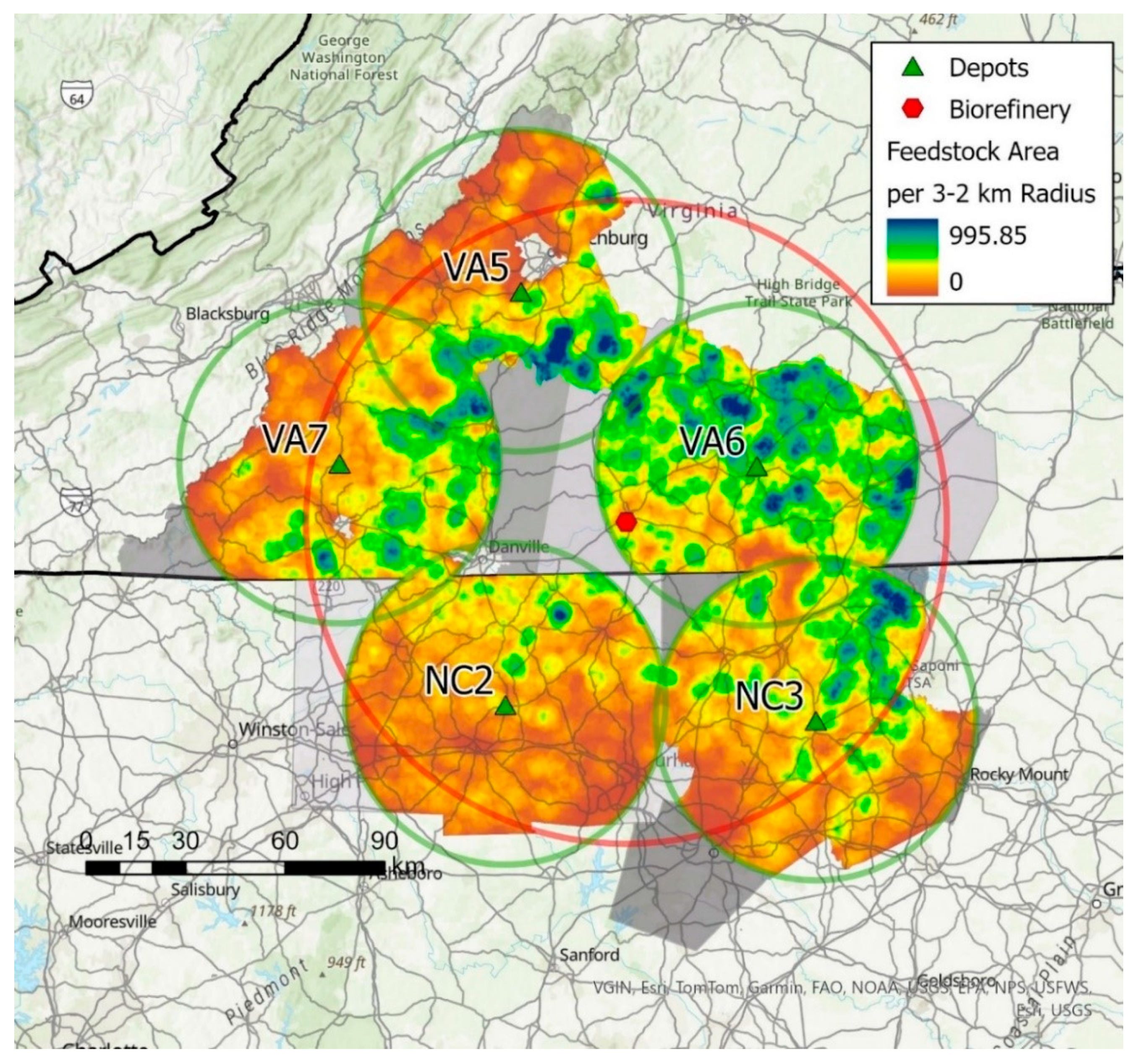
Figure 2.
Map showing location of depots for Depot-2 analysis (Depot L1 coincides with SSL 77 and Depot L2 cincides with SSL 21). Green + are SSLs.
Figure 2.
Map showing location of depots for Depot-2 analysis (Depot L1 coincides with SSL 77 and Depot L2 cincides with SSL 21). Green + are SSLs.
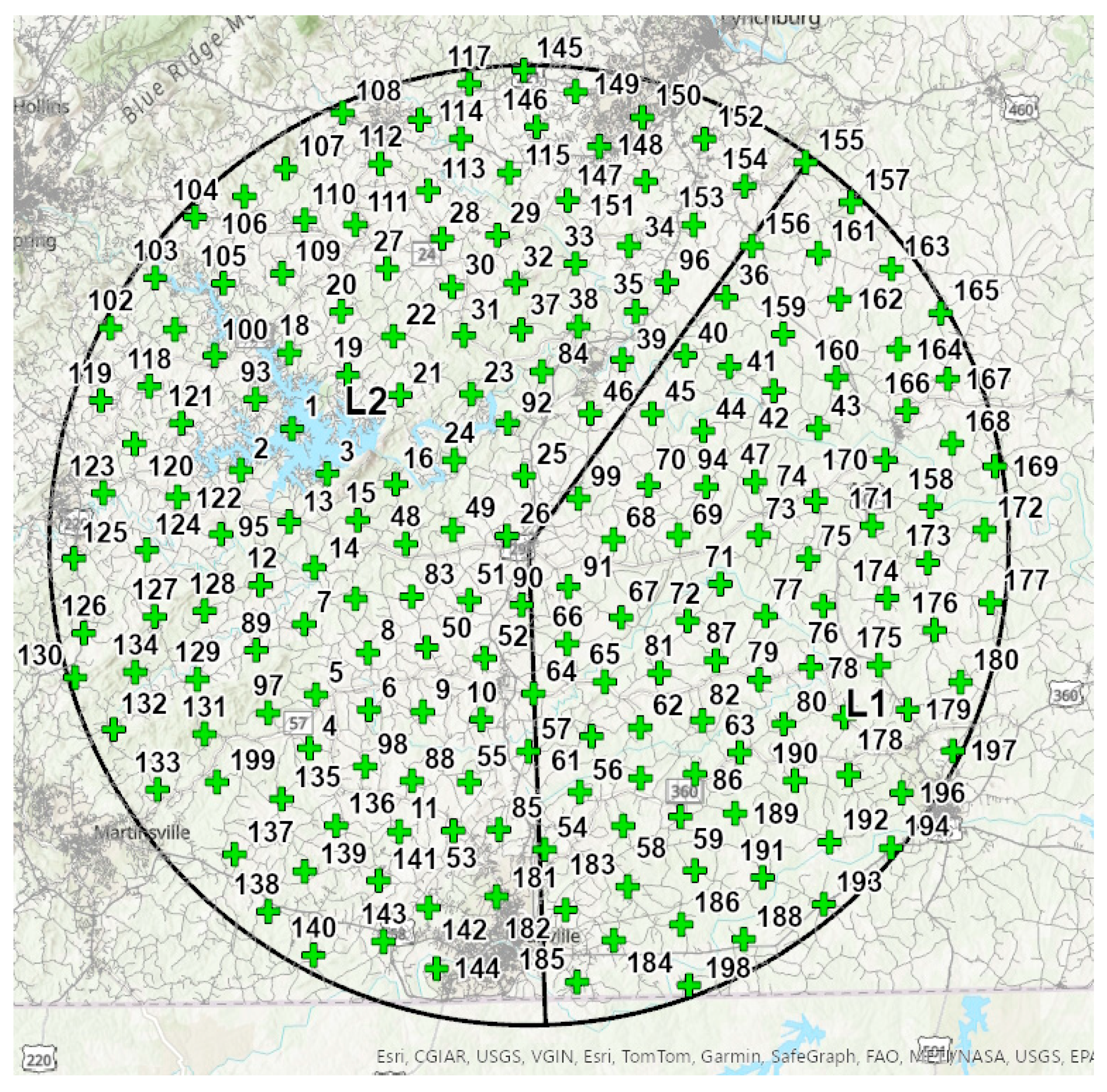
Figure 3.
Map showing location of depots (Red +) for Depot-4 analysis. Green + are SSLs.
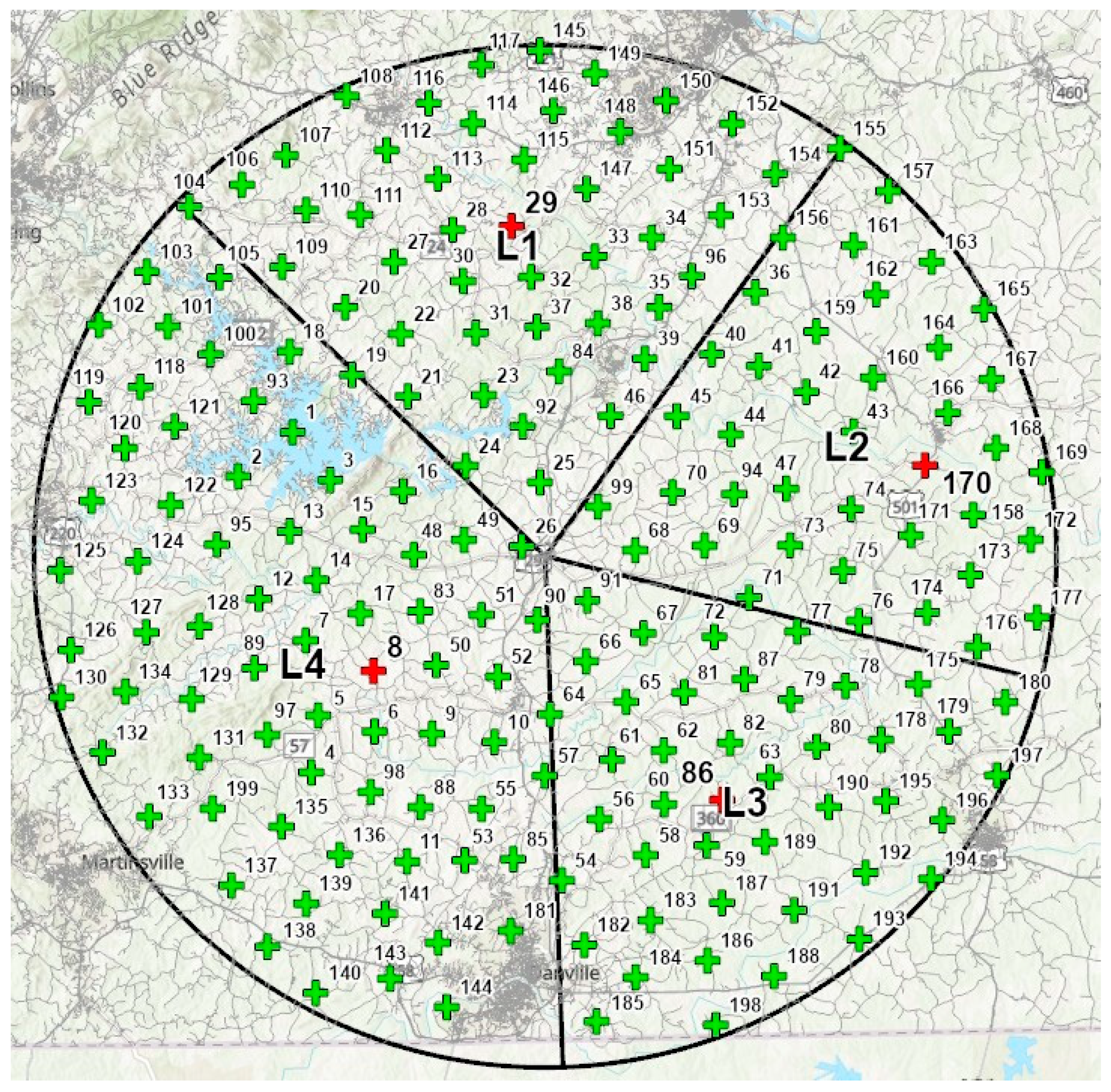
Figure 4.
Map showing highway routes for delivery of pellets from 5 depots in Depot-1 analysis.(Green triangles are the depot locations and the red dot is the biorefinery location.).
Figure 4.
Map showing highway routes for delivery of pellets from 5 depots in Depot-1 analysis.(Green triangles are the depot locations and the red dot is the biorefinery location.).
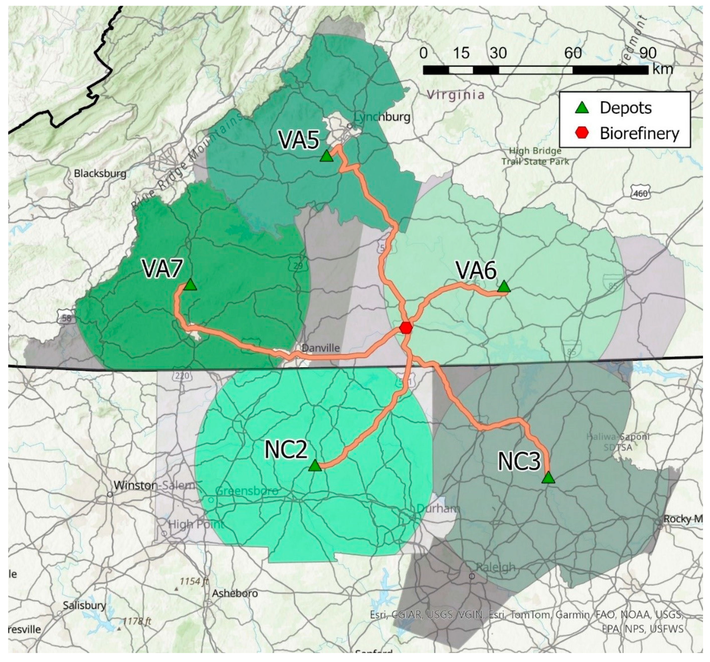
Figure 5.
Map showing highway routes for delivery of pellets from 10 depots in Depot-2 analysis. (Green triangles are the depot locations and the red dot is the biorefinery location.).
Figure 5.
Map showing highway routes for delivery of pellets from 10 depots in Depot-2 analysis. (Green triangles are the depot locations and the red dot is the biorefinery location.).
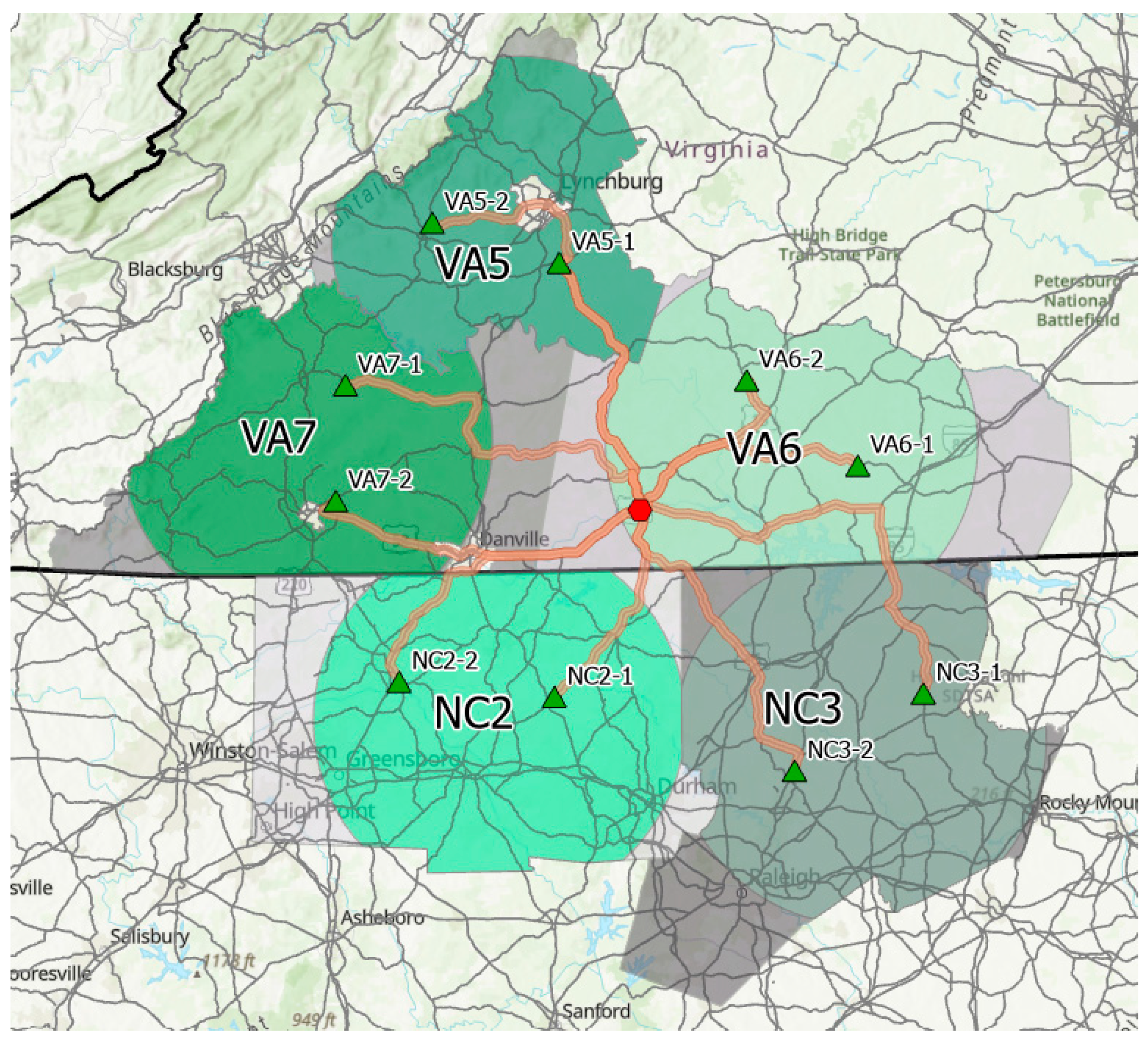
Figure 6.
Map showing highway routes for delivery of pellets from 20 depots in Depot-4 analysis. (Green triangles are the depot locations and the red dot is the biorefinery location.).
Figure 6.
Map showing highway routes for delivery of pellets from 20 depots in Depot-4 analysis. (Green triangles are the depot locations and the red dot is the biorefinery location.).
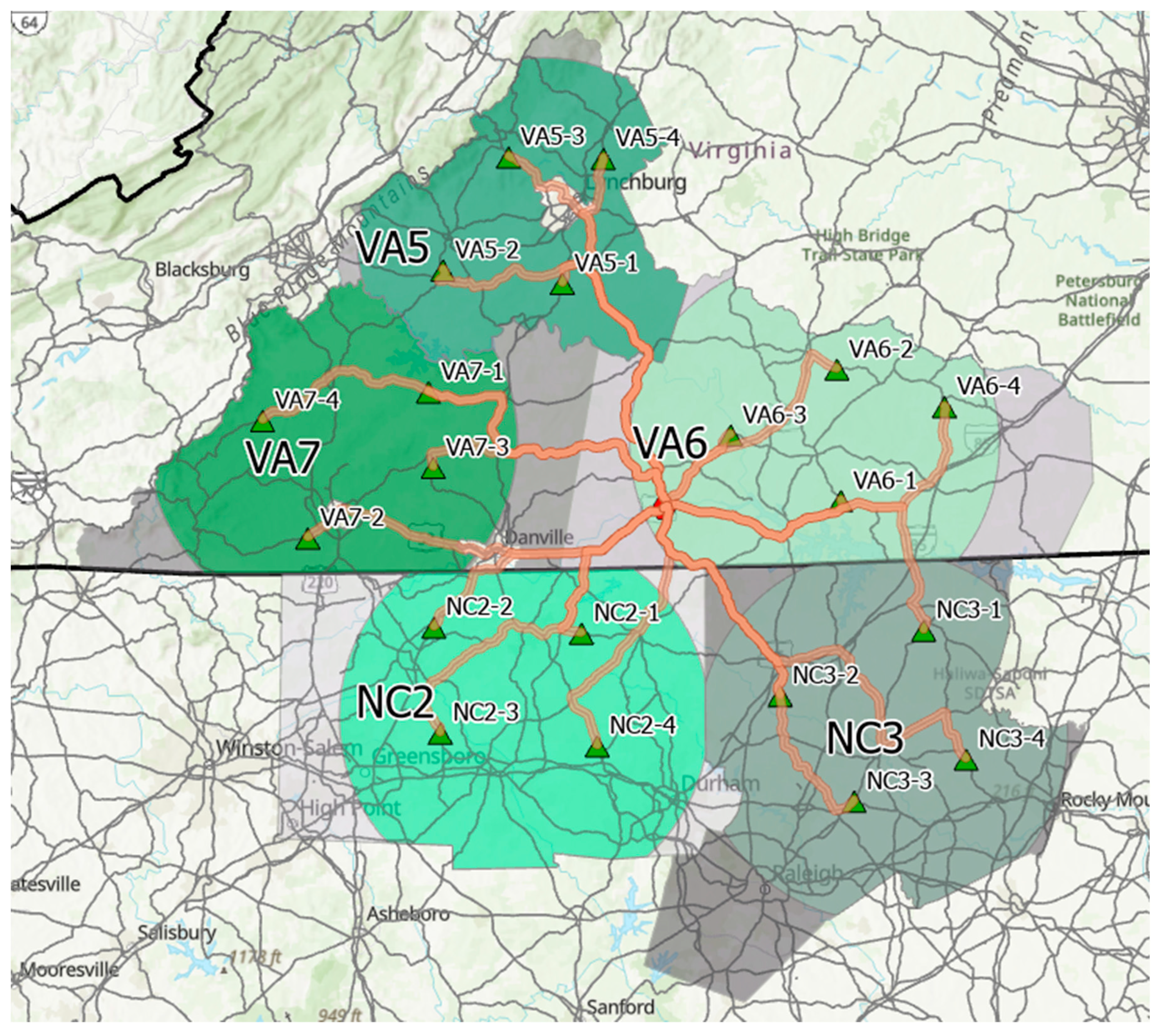

Table 1.
Total feedstock stored in five (n = 1...5) production areas (Mg at 15% MC).
| Production Area | Total Stored Biomass (Mg) |
| VA5 | 80,840 |
| VA6 | 170,830 |
| VA7 | 100,670 |
| NC2 | 80,840 |
| NC3 | 120,070 |
Table 2.
Assigned load-outs for each production area.
| Production Area | Number of Load-outs |
| VA5 | 5 |
| VA6 | 10 |
| VA7 | 7 |
| NC2 | 5 |
| NC3 | 8 |
Table 3.
Depot capacity (Mg pellets/d) for Depot-1 analysis.
| Production Area | Central Depot |
| VA5 | 197.8 |
| VA6 | 417.9 |
| VA7 | 246.3 |
| NC2 | 197.8 |
| NC3 | 298.5 |
Table 4.
Depot capacity (Mg pellets/d) for Depot-2 analysis.
| Production Area | Depot L1 | Depot L2 |
| VA5 | 99.4 | 98.4 |
| VA6 | 208.2 | 209.8 |
| VA7 | 125.7 | 120.6 |
| NC2 | 99.4 | 98.4 |
| NC3 | 151.3 | 147.2 |
Table 5.
Depot capacity (Mg pellets/d) for Depot-4 analysis.
| Production Area | Depot L1 | Depot L2 | Depot L3 | Depot L4 |
| VA5 | 50.1 | 50.3 | 49.8 | 47.7 |
| VA6 | 105.8 | 106.2 | 103.4 | 102.5 |
| VA7 | 62.4 | 63.4 | 63.1 | 57.4 |
| NC2 | 50.1 | 50.3 | 49.8 | 47.7 |
| NC3 | 75.6 | 75.9 | 76.5 | 70.6 |
Table 6.
Highway travel (km) for delivery of pellets from i = 5 depots in Depot-1 analysis.
| Production Area | Central Depot |
| VA5 | 103.7 |
| VA6 | 53.5 |
| VA7 | 120.9 |
| NC2 | 79.7 |
| NC3 | 103.6 |
Table 7.
Highway travel (km) for delivery of pellets from i = 10 depots in Depot-2 analysis.
| Production Area | Depot L1 | Depot L2 |
| VA5 | 81.2 | 134.3 |
| VA6 | 69.0 | 55.8 |
| VA7 | 112.9 | 95.0 |
| NC2 | 62.1 | 90.2 |
| NC3 | 124.2 | 95.1 |
Table 8.
Highway travel (km) for delivery of pellets from i = 20 depots in Depot-4 analysis.
| Production Area | Depot L1 | Depot L2 | Depot L3 | Depot L4 |
| VA5 | 90.5 | 129.5 | 124.3 | 111.6 |
| VA6 | 54.5 | 69.0 | 29.0 | 101.0 |
| VA7 | 96.7 | 105.1 | 84.3 | 149.7 |
| NC2 | 53.7 | 74.5 | 106.5 | 79.5 |
| NC3 | 104.5 | 68.7 | 112.9 | 140.6 |
Table 9.
Total truck operating hours to haul all raw biomass to depots for the three depot distributions.
Table 9.
Total truck operating hours to haul all raw biomass to depots for the three depot distributions.
| Production Area | Depot-1 | Depot-2 | Depot-4 |
| VA5 | 12,060 | 10,620 | 8,410 |
| VA6 | 25,840 | 22,840 | 18,070 |
| VA7 | 15,080 | 13,280 | 10,530 |
| NC2 | 12,060 | 10,620 | 8,410 |
| NC3 | 18,370 | 16,150 | 12,790 |
| Biorefinery | 83,410 | 73,510 | 58,210 |
Table 10.
Percentage decrease in truck operating hours (raw biomass hauling) relative to Depot-1 distribution.
Table 10.
Percentage decrease in truck operating hours (raw biomass hauling) relative to Depot-1 distribution.
| Production Area | Depot-2 | Depot-4 |
| VA5 | 11.9 | 30.3 |
| VA6 | 11.6 | 30.1 |
| VA7 | 11.9 | 30.2 |
| NC2 | 11.9 | 30.3 |
| NC3 | 12.1 | 30.4 |
Table 11.
Total haul distance (km)to haul all raw biomass to depots.
| Production Area | Depot-1 | Depot-2 | Depot-4 |
| VA5 | 403,930 | 331,730 | 267,170 |
| VA6 | 865,010 | 714,760 | 571,440 |
| VA7 | 504,860 | 414,815 | 331,780 |
| NC2 | 403,930 | 331,730 | 267,170 |
| NC3 | 615,030 | 503,990 | 403,090 |
| Biorefinery | 2,792,760 | 2,297,025 | 1,840,650 |
Table 12.
Total truck operating hours and total haul distance to haul pellets to the biorefinery.
| Parameter | Depot-1 | Depot-2 | Depot-4 |
| Total Operating Hours | 50,788 | 60,306 | 61,409 |
| No. Trucks Required | 8 | 9 | 9 |
| Total Truck Travel (km) | 2,006,720 | 2,388,802 | 2,441,763 |
Table 13.
Total truck operating hours, raw biomass hauling + pellet hauling, to supply biorefinery annual operation.
Table 13.
Total truck operating hours, raw biomass hauling + pellet hauling, to supply biorefinery annual operation.
| Depot | Raw Biomass | Pellet | Total |
| Distribution | Hauling | Hauling | |
| Depot-1 | 83,410 | 50,788 | 134,198 |
| Depot-2 | 73,510 | 60,306 | 133,816 |
| Depot-4 | 58,210 | 61,409 | 119,619 |
Disclaimer/Publisher’s Note: The statements, opinions and data contained in all publications are solely those of the individual author(s) and contributor(s) and not of MDPI and/or the editor(s). MDPI and/or the editor(s) disclaim responsibility for any injury to people or property resulting from any ideas, methods, instructions or products referred to in the content. |
© 2025 by the authors. Licensee MDPI, Basel, Switzerland. This article is an open access article distributed under the terms and conditions of the Creative Commons Attribution (CC BY) license (http://creativecommons.org/licenses/by/4.0/).
Copyright: This open access article is published under a Creative Commons CC BY 4.0 license, which permit the free download, distribution, and reuse, provided that the author and preprint are cited in any reuse.


