

Submitted:
12 March 2025
Posted:
13 March 2025
You are already at the latest version
Abstract
We theorize a quantum memory based on the dark-state polariton field, formed by the superposition of atomic and photonic states of a travelling probe laser pulse under the application of a standing wave modes of a dominant control laser pulse using a lambda-level scheme Electromagnetically Induced Transparency in a solid medium. We show how an enhancement in the storage time for the pulse is achieved by eliminating pulse broadening due to diffusion. At last, we propose an experiment that can help realise the storage of a probe pulse in the hyperfine levels 3H4 ↔1D2 of Pr3+: Y2SiO5, cryogenically cooled at 4.5 K. We also discuss multiple applications the storage of the quantum states the pulse probe with a prolonged time interval must have.
Keywords:
electromagnetically induced transparency
; quantum memory
; dark state polariton
; quantum computation
1. Introduction
The promise shown by quantum information as a means for computation is immense. This is primarily because of the characteristic of a quantum system. The size and complexity of the wave function, a mathematical function which represents quantum state can grow exponentially large as the number of particles in the quantum system increases. This exponential size can help us represent complex problems that a classical computer cannot. [1]Feynman was perhaps the first person to realize how much significance information processing in a quantum computer might hold in the future. He theorized how quantum laws can be simulated and understood at a deeper level in a quantum computer. [2]Any quantum algorithms of future would require reliable, robust and long-term storage solutions of quantum states, to represent information in order to process and have any significant impact on the computational landscape. It is however very difficult in practice to maintain stable quantum state over a long period of time due to quantum decoherence, pertaining to the environmental interference with a quantum system. It has been found that quantum states of photons of light are more reliable for storage purposes than any other quantum states, because of their relatively better isolation from environment and ease of manipulation for storage of information [3,4]. In this paper, we put forward a novel approach of storing and retrieving quantum information by using a quesi-particle polariton state, a mixed atomic dipole and photonic state generated by strong atom-light interaction in an electromagnetically induced transparent (EIT) ultra-cold atomic lattice ensemble.
Initial attempts at storing photonic states were very challenging and limited particularly because of the fact that any quantum state suffers from spontaneous decay from its initial state. The decoherence in turn make it challenging to use any such quantum state to encode information. One of the first attempts to use quantum states to store information was done storing states of atoms in a Zeeman ground state by coupling atomic levels with a cavity QED field and subsequent adiabatic transfer of the information of the atomic states to the states of cavity QED photons. [5] However, the cavity damping of the QED field remained a practical issue preventing the realization of a robust quantum memory architecture. The cavity damping and population loss from the atomic levels storing a quantum state was shown to be bypassed by using a three level atomic system and two coherent lasers coupling an intermediate state with lowest lifetime to an initial atomic state, in which the system is initially prepared and a final atomic state, to which the system evolves at the end of the process, storing the quantum state of the population, which was initially prepared, both states having a much longer lifetime than the intermediate state. This process was leading the populations from the initial state to the intermediate state, which then get transferred to the final state by a Stokes pulse, bypassing the spontaneous emission from the intermediate state. [6] The three level scheme to store quantum information as quantum states of an atom in an energy state was further extended to the collective atomic ensemble by the phenomenon of electromagnetically induced transparency (EIT). In this process, a quesi-quantum excitation field, composed of Raman-like atomic spin coherence states and photonic states was generated inside an atomic medium, by coupling a weaker “probe” and a stronger “control” laser between an initial ground state, at which the system is maintained initially and a final stable ground state, to which the system evolves eventually to an excited state for coherent Raman excitation of the populations. The coupling between the stable state and the excited state facilitated by the control laser splits the excited state due to which the probe laser does not get absorbed by the atomic medium, instead the photonic states of the laser get transferred to the collective atomic excitation of the medium, culminating in the stable state creating a ‘dark state’ The dark state is a superposition state of the initial state and the final stable state and therefore remain from the spontaneous emission. When such an atomic ensemble couples to a strong control cavity QED field, and reaches the collective dark state, the quantum state of the probe pulse gets stored in the atomic spin excitation of the final stable ground state, creating a superposition of the photonic and the atomic spin excitation state, known as ‘dark state polariton’. [7] The coherence of the spin atomic excitation was shown enhanced by manipulation of the dispersion of the atomic medium by application of two counter-direction control lasers coupling the final stable state with the excited state. By the effect of these lasers, a standing wave is generated in the atomic medium, which creates a band gap in the band structure of the atomic medium, facilitating trapping of the probe pulse inside the medium as a standing wave probe. [8] The effect of the standing wave probe inside the medium showed a greater coherence time for the quantum state stored inside it and hence provided a window of possibility to have more stable and robust quantum memories [9,10,11]. It was theoretically shown how the counterpropagating control lasers eliminate total dispersion loss of the quantum state, stored as a perfectly standing wave probe field inside an EIT medium. [12]
The trapped standing wave probe field can be a potent quantum memory in the future quantum computers. The retrieval of information as photonic state of the probe, however, requires one of the counter-directional lasers to be shut off for the probe to be retrieved by a photon detector in that particular direction, desired. It can be inferred that the elimination of the dispersion loss will not be present while the retrieval of the stored standing wave pulse as a travelling wave pulse is in progress inside the atomic medium. So, in fact the retrieved information about the quantum state will still not be free from environmental interference and will suffer incoherent losses. Therefore, the retrieval and propagation of the probe pulse inside the atomic medium as a polariton excitation, also demands shielding from the eminent diffusion losses, due to the diffusive motion of the atoms. It has already been shown that counter-directional control laser driven EIT system in the frequency-up conversion regime provide much better transparency windows to travelling probe pulse inside the medium, than travelling wave control laser field. In this paper, we put forward an adiabatic technique to address the issue by extending the shielding effect of the standing wave control field from the dispersion losses in the standing wave probe inside an EIT medium to the travelling probe as well and compare their effects with the travelling wave control field case. We present with an adiabatic Raman population transfer technique of EIT, by incorporating the effects of a standing wave control laser QED field on a travelling wave probe in an ensemble, composed of stationary atoms. We derive the propagation equation for the travelling probe field inside the EIT medium and show how the Fourier modes of the standing wave control laser field eliminate the diffusion loss in the travelling probe as well. We also propose an experiment to show how the storage of travelling probe pulse can be realized in a stationary atomic medium such as a rare-earth doped crystal lattice of Pr3+: Y2SiO5 by creation of an EIT system, using a Dye laser to couple the hyperfine levels 3H4 ↔1D2 of the crystal, having a very long lifetime.
2. Methodology
Our system is implemented using a solid crystalline atomic medium, structured as an ensemble lattice of atoms. We employ a lambda-level Electromagnetically Induced Transparency (EIT) scheme, wherein two hyperfine components of the ground-state energy levels are connected to an excited atomic state. Specifically, two strong counterpropagating coupling lasers, referred to as control lasers, with Rabi frequency , couple the final stable ground-state component to the excited state ∣a⟩. Concurrently, a weak coupling laser, referred to as the probe laser, links the initial ground-state component ∣b⟩ with the same excited state ∣a⟩. Notably, the direct transition between the two ground-state components ∣b⟩ and ∣c⟩ is forbidden. The system leverages quantum interference effects: the destructive interference of transition probability amplitudes for the transitions ∣b⟩→∣a⟩ and ∣c⟩→∣a⟩. This interference enables the probe laser pulse to propagate through the medium without significant absorption. Furthermore, the wave vectors of the probe and control lasers are configured to satisfy the velocity-tuned multiphoton processes, ensuring coherent coupling and efficient EIT dynamics. This configuration is crucial for achieving the desired transparency and enhanced control over light-matter interactions within the medium.
Figure 1.
A Lambda Level EIT System, where counter-propagating control lasers with amplitude and a probe laser with amplitude and are the detunings.
Figure 1.
A Lambda Level EIT System, where counter-propagating control lasers with amplitude and a probe laser with amplitude and are the detunings.
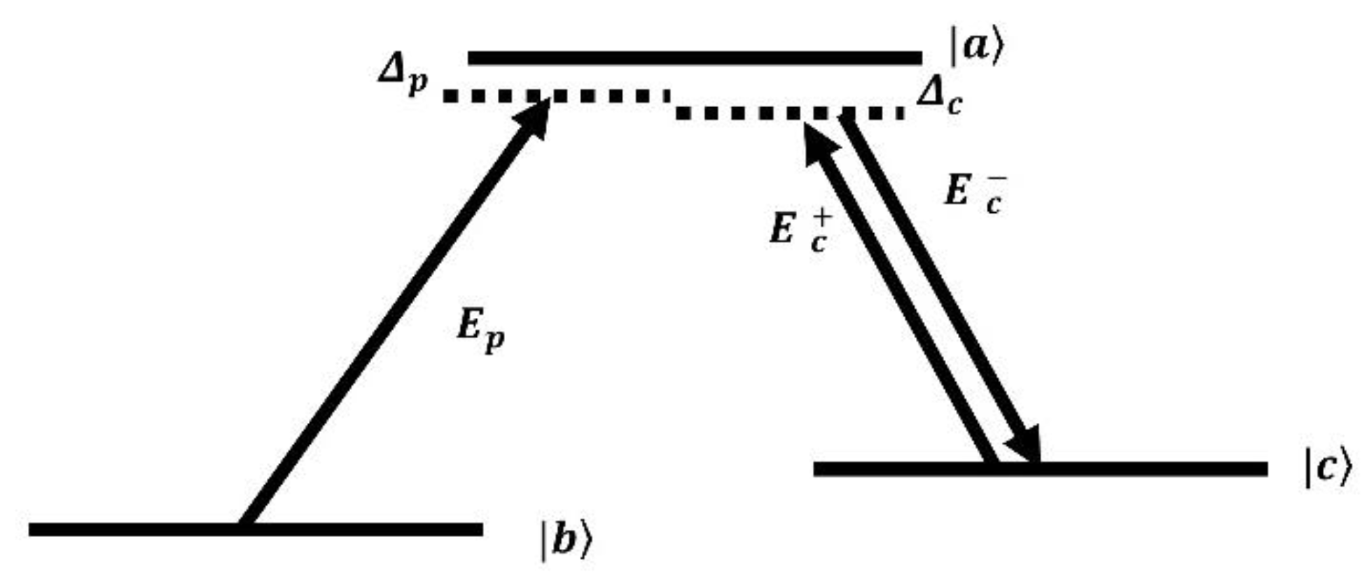
Here, ‘q’ represents the number of photons in the control laser pulse, while v denotes the atomic velocity. The detunings of the probe and control laser pulses are denoted by Δp and Δc, respectively. We consider a system comprising N lambda-level atoms interacting with two distinct laser fields: a standing-wave control laser field with amplitude Ec± and wave vector ±kc, and a traveling-wave probe field with amplitude Ep and wave vector kp. The atomic states are described using density matrix elements , while denotes the dipole operators. For simplicity, we assume the atomic velocity v to be approximately zero, consistent with the ensemble configuration of our atomic lattice system. However, we acknowledge the presence of atomic diffusion in real lattice systems, where v cannot be strictly zero. To further simplify the model, we consider near-resonant conditions for both the probe and control laser fields, such that Δp ≈ 0 and Δc ≈ 0. Under these assumptions, the Hamiltonian describing the interaction of the N-atom lambda-level system is expressed as follows:
This formulation provides a foundation for analysing the coherent dynamics and light-matter interactions within the atomic lattice under the specified EIT scheme. In the presence of laser-atom interaction, we assume that the time evolution of the atomic operators is slow compared to the timescale of the electromagnetic fields. This allows us to define slowly varying atomic elements for the analysis. Specifically, we define , and and are unit vectors along the propagation directions of the control and probe lasers, respectively. Additionally, the slowly varying atomic density matrix elements are denoted as , in contrast to the standard atomic density matrix elements . Substituting the slowly varying atomic elements into Heisenberg’s equation of motion and applying the rotating wave approximation (RWA), which eliminates rapidly varying terms, we derive the Heisenberg-Langevin equations of motion. Here, represents the incoherent decay rates of the electron population in specific states.
Given that the probe pulse is significantly weaker than the standing-wave control laser fields, the equations can be solved using a perturbative approach, as outlined in [13]. In this method, the atomic density matrix elements are expanded in powers of ϵ, defined as the ratio of the amplitudes of the probe and control pulses. Under the initial condition that the majority of atoms are in the ground state ) , the atomic density matrix elements are obtained as follows:
Here, . where Ωc± are the control field components. The equations of motion derived in this framework, such as (3a), (3b), and (3c), evolve very slowly. To account for this, we define the characteristic timescale of laser operation as . The slowly varying atomic operator is expanded in powers of . Expanding up to zeroth order in Equation (3c) and substituting into Equation (3a), we derive the following:
By inserting the value of in Equation 4(a), we get:
Rewriting these equations using the definitions , we find the spin excitation of the probe where is the total Rabi frequency of the control field, and represents a constant phase.
We must also know the wave-equation of the electromagnetic field in an atomic medium. It has been shown that the wave equation can be written as: [13]
Having derived the atomic spin excitation operator for our atomic ensemble, we are now in a position to review in detail, how theses spin excitation helps quantum state to be stored as quantum information. In this study, we consider a system where all atoms are initially prepared in the ground state ∣b,0⟩. Under this condition, the interaction couples the system exclusively to the totally symmetric Dicke-like states. Specifically, if the field is prepared in an initial state containing at most one photon, the relevant eigenstates of the bare system are as follows: The total ground state ∣b,0⟩, which remains unaffected by the interaction. The ground state with a single photon in the field, ∣b,1⟩. The singly excited atomic states ∣a,0⟩ and ∣c,0⟩. These states form the basis of the interaction dynamics, with the system transitioning among them under the influence of the laser fields. The exclusion of other states simplifies the analysis and highlights the key physical processes associated with single-photon and single-atom excitations in the system. [13]
The eigenstates of the Hamiltonian in Equation (1) can be found as
can be identified as the required dark state, which we already discussed in the Introduction. For the ensemble the dark state for a single photonic excitation can be given as: . Here, is defined as the mixing angle. For n such excitations the expression can be given as:[13]
By adiabatic rotation of the mixing angle , from 0 to π/2 leads to reversible transfer of the photonic number states to the collective atomic spin excitations stored at the final stable state [13]
The operation generates a tensor product mix of the photonic states and the collective atomic spin excitations as [13]
The formulation presented above is based on the time-independent version of the Hamiltonian at (1), however to derive the propagation equations of the probe inside the atomic ensemble with the preserved quantum states in the atomic excitation, we need to work with the time dependent dynamics of the above system, featuring a time dependent control field. Consequently, the atomic excitation derived in the Equations 4(a)-4(c) will also have to be time dependent. Please note we need to solve the coupled equations (4(c) ) and (5) to solve the propagation problem. Physically, this means we calculate how the atomic excitation evolves as the electromagnetic field of the probe propagates inside the atomic ensemble. To perform the time dependent calculations effectively we need to arrive at a single equation, which can predict the time dependence of both the atomic operator and the electromagnetic field. To solve the problem, a quesi-particle called ‘dark state polariton’ was introduced in [13]. The quantum field is defined as the linear superposition of the bosonic field (in our case probe laser electromagnetic field and an atomic excitation operator field allowing the above dark state transitions.
These field operators follow bosonic commutation relations.
The dark state transition then can be written as being the vacuum state, i.e.: . Now we are ready to derive the propagation equations for the polariton fields. For including the atomic diffusion into the polariton picture the propagation equation for the dark polariton field need to be of second order in special coordinate. For that we expand 3 (c) up to first order in , and then insert the value of in 4(a), we thus get
By using the definition of the polariton field in (7) we get
The wave equation for the probe field then can be written in terms of the dark polariton field, considering constant mixing angle as:
In a solid-state system, the atomic operators exhibit vibrations corresponding to all possible wave vectors, enabling their representation as a Fourier series. These vibrations correspond to the complete set of standing wave modes of the control field within the cavity. The interaction between the atomic spin excitation field operators and these modes gives rise to polaritons, which encode the quantum state of the probe pulse photons. Therefore, the denominator appearing on the right-hand side of Equation (10) can similarly be expressed as a Fourier series.
Substituting the fourier expansion of the denominator in (10) we get:
The propagation equation for the spin excitation operator is derived, by finding the correct Fourier coefficient, for which the unidirectional polariton component have the corresponding primary Fourier mode of the spin excitation (i.e.:. The Fourier coefficients are given as [12]:
The final propagation wave equation for the travelling probe obtained after evaluating Equation (12) further, considering a very low decoherence rate and using the relation between the second order derivative of space and time coordinates will be as follows
As we have chosen a stationary atomic system, only first order Fourier coefficients are of significance as they are much larger than the higher order Fourier coefficients, so we only need to find the as we are considering the special case of using Equation (13 a) and (13 b): . Substituting the Fourier coefficients in Equation(14), approximating the group velocity and evaluating we get :
The wave equation governing the polariton fields under non-adiabatic conditions is presented, incorporating a second-order derivative term on the right-hand side. This term, identified as the diffusion term, arises from pulse broadening, which leads to the loss of polariton fields stored within the material as quantum memory. The term diminishes due to the standing wave control field Rabi frequencies. The equation is solved using the Fourier transform method, yielding a solution in Fourier space after integrating both sides. Assuming an initial Gaussian probe wave, expressed as , selecting units where for simplicity and choosing the group velocity’s time dependence as , where is the characteristic switching time of the laser, the solution is subsequently transformed back to real space via an inverse Fourier transform. The resulting expression, obtained numerically, provides insight into the behavior of the polariton field under the given conditions:
The total energy density obtained after substituting in terms of field amplitude based on the definition (7) is:
The total energy density derived under the given conditions reveals that, for a perfect standing wave configuration the diffusion term on the right-hand side of the wave equation vanishes entirely.
In this scenario, there is no energy loss attributable to diffusion, although losses arising from decoherence may still persist. This result highlights the significance of the standing wave configuration in minimizing diffusion-related losses in the system. This feature has been previously demonstrated for a standing wave probe pulse trapped inside an EIT cavity. Our results extend this understanding by showing that diffusion losses of a traveling probe pulse inside an EIT cavity can also be minimized by the primary modes of the standing wave control field. The application of the standing wave control field reduces the traveling probe field losses, leading to extended coherence and storage times. However, our formulation assumes that the spontaneous downward transition of atoms in the dark state is negligible compared to the atomic population at that level. In a real atomic system, the spontaneous downward transition is significant and must be considered. This transition follows an exponential decay law, and incorporating the loss due to spontaneous emission allows the energy density derived earlier to be approximately recalculated as:
3. Proposed Experimental Validation
Several experiments have demonstrated the use of standing wave control fields to create an Electromagnetically Induced Transparency (EIT) window for standing wave pulses in atomic systems. However, only a few studies have focused on stationary solid-state atomic systems. Our proposed experiment aims to explore EIT-based quantum memory storage in a cryogenically cooled (4.5 K) rare-earth-doped Pr³⁺:Y₂SiO₅ crystal. Building on the work of G. Heinze et al. (2013) and D. Schraft et al. (2016), who achieved high storage efficiencies (optical depth ~96) and extended storage times (up to one minute) using traveling wave control fields, we propose a new approach utilizing a standing wave control field. Specifically, we will employ two counterpropagating control laser fields through the crystal to create a standing wave pattern [14,15]. The experiment uses the hyperfine levels 3H4 ↔1D2, of Pr3+: Y2SiO5 to form a Λ-level EIT system. A frequency-stabilized laser with a bandwidth below 100 kHz (FWHM) on a 100 ms timescale will generate preparation, control, and probe pulses. Acousto-optic modulators (AOMs) will modulate pulse intensities and frequencies. The preparation sequence involves optical pumping and repumping to prepare the atomic population in the ground state. A preparation pulse with a spectral range of 0<Δν<18 MHz and a duration of 84 ms will create a spectral pit in the absorption medium. Repumping the two hyperfine components of the ground state 3H4 will involve a short pulse of 30 ms duration with a relative frequency of +25.7 MHz. A cleaning pulse of 100 μs will remove residual excited-state population [16,17]. The experimental setup, as shown in Figure 2, uses probe and control pulses derived from a dye laser, passed through single-mode optical fibers. A beam splitter (BS1) separates the pulses into a weak probe beam and a control beam. The control beam is further split using another beam splitter (BS2) to generate a standing wave control field. The probe pulse is directed onto the Pr³⁺:Y₂SiO₅ crystal using reflective mirrors and alignment telescopes, while the counterpropagating control beams focus on the crystal with minimal angular separation. Polarizing beam splitters (PBS) and AOMs polarize and fine-tune the beams’ intensity and frequency. Initially, only the control beams are applied to create a standing wave within the crystal. After a microsecond delay, the probe pulse is introduced, inducing EIT in the medium. This reduces the group velocity of the probe to near zero, forming a dark-state polariton—a coherent superposition of atomic states. The standing wave control field minimizes diffusion losses, enabling efficient quantum memory storage within the adiabatic time limit. The storage duration is governed by the hyperfine level lifetimes, with the stored probe pulse retrievable by turning off the control field, completing the memory cycle.
4. Results
Equation (16) highlights the critical role of the Rabi frequencies of counter-propagating control lasers in shaping the traveling dark-state polariton (DSP) waveform. The counter-propagating laser pulses generate cavity modes that are inherently dependent on these Rabi frequencies, which, in turn, influence the EIT window through which the traveling probe polariton propagates. By varying the control laser fields, the Fourier modes of the control lasers can be adjusted, allowing precise manipulation of the probe pulse’s shape and duration. This tunability facilitates the manipulation of photonic quantum states within the atomic medium as polaritons, making them highly suitable for quantum memory applications that require extended coherence times. Different ratios of result in either enhanced or diminished waveforms of the probe polariton field. Notably, when counter-propagating control fields of equal intensities are applied, the polariton field stored within the crystal experiences no diffusion loss. Under these optimal conditions, the adiabatic storage of the probe pulse is limited solely by the spontaneous emission rates of the ground-level hyperfine states & , ensuring high-fidelity quantum memory storage.
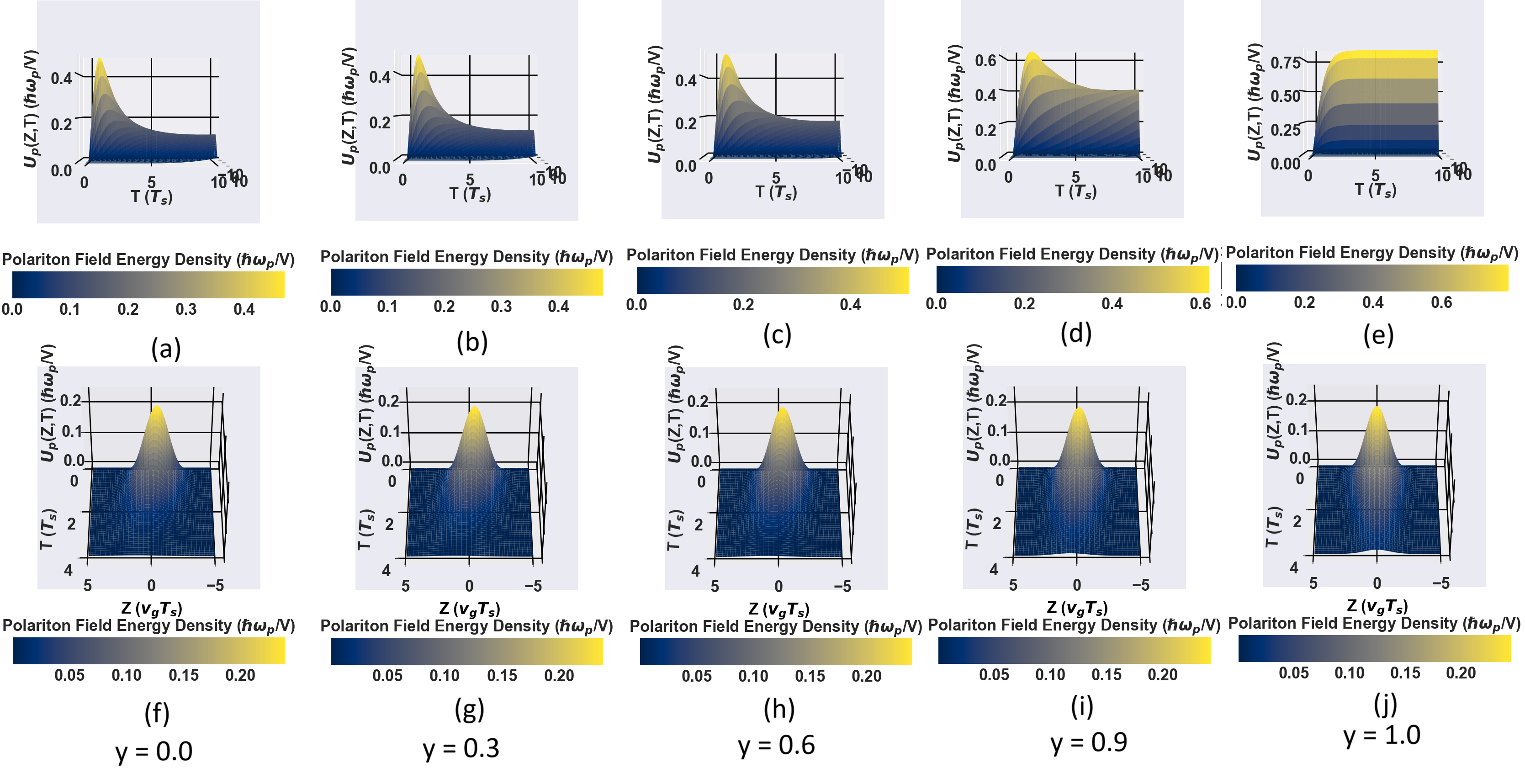
Figure 3 (a)-(e) illustrates the energy decay of the polariton field under various control field configurations. In the case of a traveling wave control field (y=0.0), the polariton energy exhibits exponential decay due to diffusion losses. With counter-propagating control fields (y=0.3-0.9), the diffusion losses are significantly reduced, resulting in a slower decay of the polariton field energy and an extended coherence time for the photonic states mapped into atomic states. For a perfectly standing wave control field (y=1.0), diffusion losses are completely eliminated, and the polariton energy remains constant over time in the absence of spontaneous emission. This configuration ensures that the collective atomic excitations remain undisturbed, theoretically enabling indefinite storage. However, in real atomic systems, the finite spontaneous emission rate imposes a practical limitation on the storage duration. Figure 3 (f)-(j) illustrates the effect of the standing wave control on the pulse broadening of the probe pulse inside the medium. As we approach the perfectly standing probe pulse condition, pulse broadening decreases and gets eliminated completely when perfectly standing wave control field is obtained.
Figure 4 illustrates the variation in pulse broadening of the polariton with the Rabi frequency ratio, . In the traveling wave control field configuration (y=0), the Full Width at Half Maximum (FWHM) of the polariton energy density distribution is the largest, indicating significant pulse broadening caused by diffusion-induced expansion. In contrast, for counter-propagating control fields (y=0.3-0.9), the FWHM decreases as diffusion losses are reduced, resulting in a narrower pulse width. The perfectly standing wave control field case (y=1) demonstrates the smallest FWHM, reflecting minimal pulse broadening due to the complete elimination of diffusion loss.
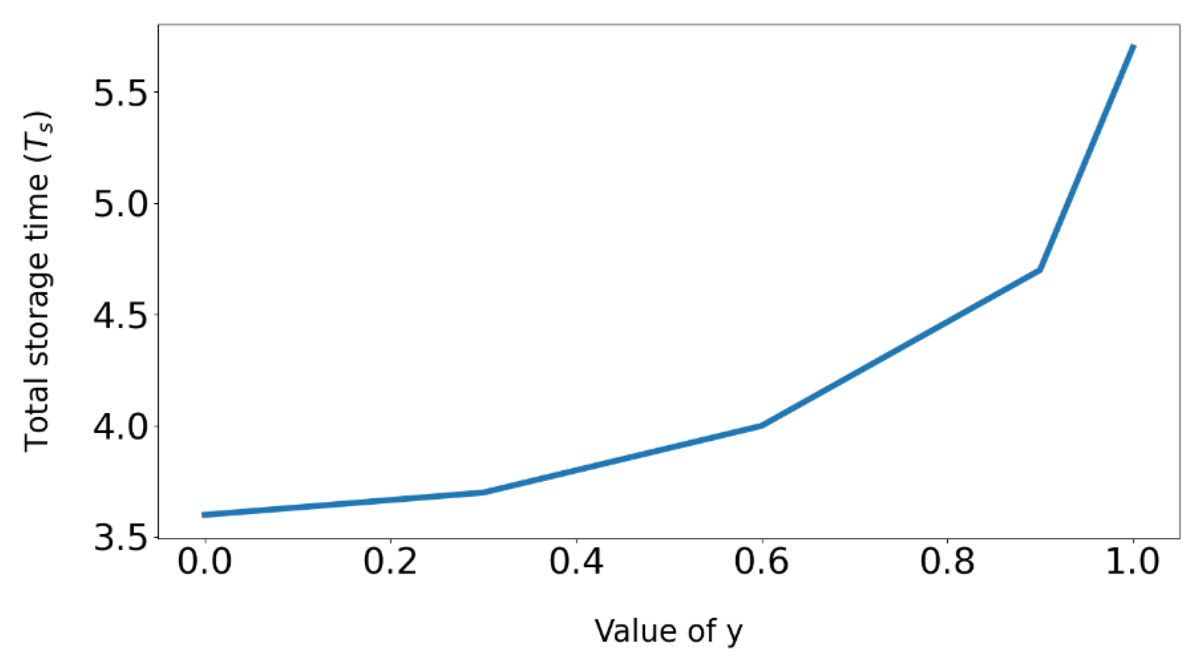
Figure 5 illustrates the perfectly standing wave control field the storage duration of the probe pulse is significantly extended compared to the traveling wave case , based on the time taken for the energy density to fall below 0.01, the storage time increases from approximately T ~ 3.6 Ts for the traveling wave case to T ~ 5.7 Ts for the standing wave case. Here, Ts represents the switching time of the control laser. These results highlight the advantages of the standing wave control field, which significantly prolongs the storage time of the probe field within the crystal, limited only by the lifetime of the ground state 3H4. This makes the standing wave configuration a superior choice for quantum memory applications.
5. Conclusion
Quantum computers are being envisioned—and increasingly applied—in a wide array of fields, from the use of quantum cryptography in cybersecurity to the potential for quantum simulations in quantum chemistry for chemical engineering applications. [18]One of the most intriguing prospects that has recently captured researchers’ attention is the scalability of machine learning models to unprecedented levels, enabled by the significantly faster learning capabilities of quantum computers compared to classical systems [19,20,21]. However, the realization of such advanced quantum algorithms relies critically on the availability of reliable, robust, and long-term quantum state storage solutions, which are essential for quantum computing to make a transformative impact on the computational landscape. The quantum memory storage process by utilization of the transparency window, provided by electromagnetically induced transparency, as described in this paper can prove to be very effective for such purpose. One of the other potential areas of research in the future is processing of exponential amount of classical information by quantum computers. A potent solution to such a problem has already been provided by Giovannetti, in which he proposed a quantum version of volatile short-term memory such as classical RAM can be realized using various procedures involving phase gates, qutrits and entanglement [22,23,24]. Quantum memory using trapped photonic states inside an EIT medium can prove very effective in realizing memory cells in such a Q-RAM scheme, pertaining to the quality of photonic states being much less susceptible to environmental interference and being easy to manipulate. Also, quantum state retrieval using a probe pulse from the address shells in Q-RAM schemes, built upon multiple EIT systems can feature greater fidelity. Our analysis demonstrates that standing wave control laser fields significantly enhance the coherence times of traveling probe laser pulses in solid crystalline atomic systems, enabling extended storage durations for the quantum state of photons. Notably, these storage times are independent of the intrinsic properties of the solid-state atomic medium and are instead governed by controllable parameters, such as the ratio of the Rabi frequencies of the counter-propagating control lasers. While prior studies primarily focused on eliminating diffusion losses and improving coherence times for stationary pulses, our work extends these benefits to traveling probe pulses. The observed increase in coherence time, as evidenced by the temporal profile Up(z,t), results from the broader absorptive range of the control field wave vector in the standing wave configuration compared to the traveling wave ca se. We have also proposed an experimental setup to implement the standing wave control laser field EIT system and investigate the storage of traveling probe pulses in a cryogenically cooled (4.5 K) Pr:YSO crystal. While the storage of stationary pulses has been extensively studied in warm and cold atomic gases, the application of counter-propagating control fields to store traveling pulses in solid-state media remains largely unexplored. Recently, Hain et al. (2022) demonstrated the storage of a traveling photon pulse using a traveling wave control field for up to 100 seconds in the 3H4 ↔1D2 levels of Pr:YSO . [25]Building upon this work, our proposed experiment predicts longer coherence times for stored pulses using standing wave control fields, as supported by our theoretical model. Despite these advancements, storage durations remain fundamentally constrained by spontaneous emission. Future research must explore innovative strategies to mitigate these limitations and extend the storage capabilities of optical memories beyond current theoretical boundaries. Addressing these challenges could significantly enhance the performance of optical memories, making them practical for a wider range of applications in quantum technologies.
References
- I. Krylov, J. Doyle and K.-K. Ni, “Quantum computing and quantum information storage,” Phys. Chem. Chem. Phys., vol. 23, no. 11, pp. 6341-6343, 2021.
- R. P. Feynman, “Simulating physics with computers,” International Journal of Theoretical Physics, vol. 21, pp. 467-488, 1982.
- J. L. O’Brien, G. J. Pryde, A. G. White, T. C. Ralph and D. Branning, “Demonstration of an all-optical quantum controlled-NOT gate,” Nature, vol. 426, pp. 264-267, 2003.
- D. Petrosyan, “Towards deterministic optical quantum computation with coherently driven atomic ensembles,” Journal of Optics B: Quantum and Semiclassical Optics, vol. 7, p. S141, 2005.
- A. S. Parkins, P. Marte, P. Zoller and H. J. Kimble, “Synthesis of arbitrary quantum states via adiabatic transfer of Zeeman coherence,” Phys. Rev. Lett., vol. 71, no. 19, p. 3095–3098. 19 November.
- K. Bergmann, H. Theuer and B. W. Shore, “Coherent population transfer among quantum states of atoms and molecules,” Rev. Mod. Phys., vol. 70, no. 3, p. 1003–1025, July 1998.
- M. Fleischhauer and M. D. Lukin, “Dark-State Polaritons in Electromagnetically Induced Transparency,” Phys. Rev. Lett., vol. 84, no. 22, p. 5094–5097, May 2000.
- A. André and M. D. Lukin, “Manipulating Light Pulses via Dynamically Controlled Photonic Band gap,” Phys. Rev. Lett., vol. 89, no. 14, p. 143602, September 2002.
- M. Bajcsy, A. S. Zibrov and M. D. Lukin, “Stationary pulses of light in an atomic medium,” Nature, vol. 426, p. 638–641, 2003.
- F. E. Zimmer, A. André, M. D. Lukin and M. Fleischhauer, “Coherent control of stationary light pulses,” Optics Communications, vol. 264, pp. 441-453, 2006.
- A. André, M. Bajcsy, A. S. Zibrov and M. D. Lukin, “Nonlinear Optics with Stationary Pulses of Light,” Phys. Rev. Lett., vol. 94, no. 6, p. 063902, February 2005.
- K. R. Hansen and K. Mølmer, “Trapping of light pulses in ensembles of stationary Lambda atoms,” Phys. Rev. A, vol. 75, no. 5, p. 053802, May 2007.
- M. Fleischhauer and M. D. Lukin, “Quantum memory for photons: Dark-state polaritons,” Phys. Rev. A, vol. 65, no. 2, p. 022314, January 2002.
- G. Heinze, C. Hubrich and T. Halfmann, “Stopped Light and Image Storage by Electromagnetically Induced Transparency up to the Regime of One Minute,” Phys. Rev. Lett., vol. 111, no. 3, p. 033601, July 2013.
- D. Schraft, M. Hain, N. Lorenz and T. Halfmann, “Stopped Light at High Storage Efficiency in a Pr³⁺:Y₂SiO₅ Crystal,” Phys. Rev. Lett., vol. 116, no. 7, p. 073602, February 2016.
- F. Beil, J. Klein, G. Nikoghosyan and T. Halfmann, “Electromagnetically induced transparency and retrieval of light pulses in a Λ-type and a V-type level scheme in Pr³⁺:Y₂SiO₅,” Journal of Physics B: Atomic, Molecular and Optical Physics, vol. 41, p. 074001, March 2008.
- M. Nilsson, L. Rippe, S. Kröll, R. Klieber and D. Suter, “Hole-burning techniques for isolation and study of individual hyperfine transitions in inhomogeneously broadened solids demonstrated in Pr³⁺:Y₂SiO₅,” Phys. Rev. B, vol. 70, no. 21, p. 214116, December 2004.
- F. Bova, A. Goldfarb and R. G. Melko, “Commercial applications of quantum computing,” EPJ Quantum Technology, vol. 8, p. 2, 2021.
- S. Aaronson, “Read the fine print,” Nature Physics, vol. 11, pp. 291-293, 2015.
- A. W. Harrow, A. Hassidim and S. Lloyd, “Quantum Algorithm for Linear Systems of Equations,” Physical Review Letters, vol. 103, p. 150502, 2009.
- S. Lloyd, M. Mohseni and P. Rebentrost, “Quantum algorithms for supervised and unsupervised machine learning,” arXiv: Quantum Physics, 2013.
- V. Giovannetti, S. Lloyd and L. Maccone, “Architectures for a quantum random access memory,” Physical Review A, vol. 78, p. 052310, 2008.
- V. Giovannetti, S. Lloyd and L. Maccone, “Quantum Private Queries,” Physical Review Letters, vol. 100, p. 230502, 2008.
- V. Giovannetti, S. Lloyd and L. Maccone, “Quantum Random Access Memory,” Physical Review Letters, vol. 100, p. 160501, 2008.
- M. Hain, M. Stabel and T. Halfmann, “Few-photon storage on a second timescale by electromagnetically induced transparency in a doped solid,” New Journal of Physics, vol. 24, p. 023012, February 2022.
Figure 2.
Proposed experimental setup for standing wave control field EIT-based quantum memory storage.
Figure 2.
Proposed experimental setup for standing wave control field EIT-based quantum memory storage.
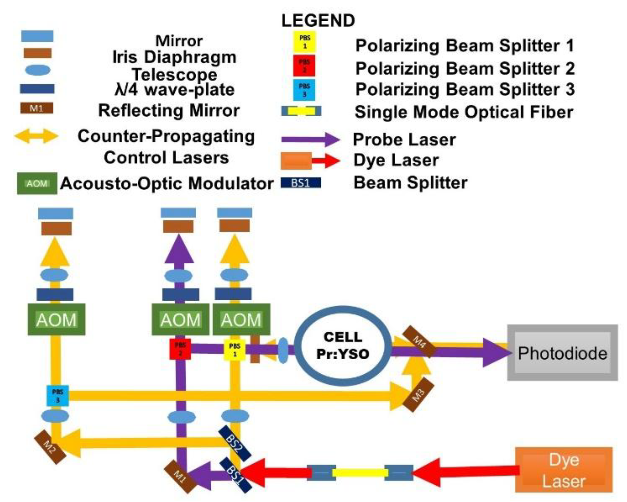
Figure 3.
(a)-(e) Plots of total polariton field energy density of the probe pulse showing the temporal variation in arbitrary units without considering spontaneous emission loss (f)-(j) Plots of total polariton field energy density of the probe pulse showing the pulse broadening in spatial units, considering spontaneous emission loss The plots ranges from y = 0.0 (travelling wave control field case) up to y= 1.0 (perfectly standing wave control field case).Here, .We have chosen the constants: , time T is in units of , energy is in units of , distance z is in units of , energy is in units of .
Figure 3.
(a)-(e) Plots of total polariton field energy density of the probe pulse showing the temporal variation in arbitrary units without considering spontaneous emission loss (f)-(j) Plots of total polariton field energy density of the probe pulse showing the pulse broadening in spatial units, considering spontaneous emission loss The plots ranges from y = 0.0 (travelling wave control field case) up to y= 1.0 (perfectly standing wave control field case).Here, .We have chosen the constants: , time T is in units of , energy is in units of , distance z is in units of , energy is in units of .
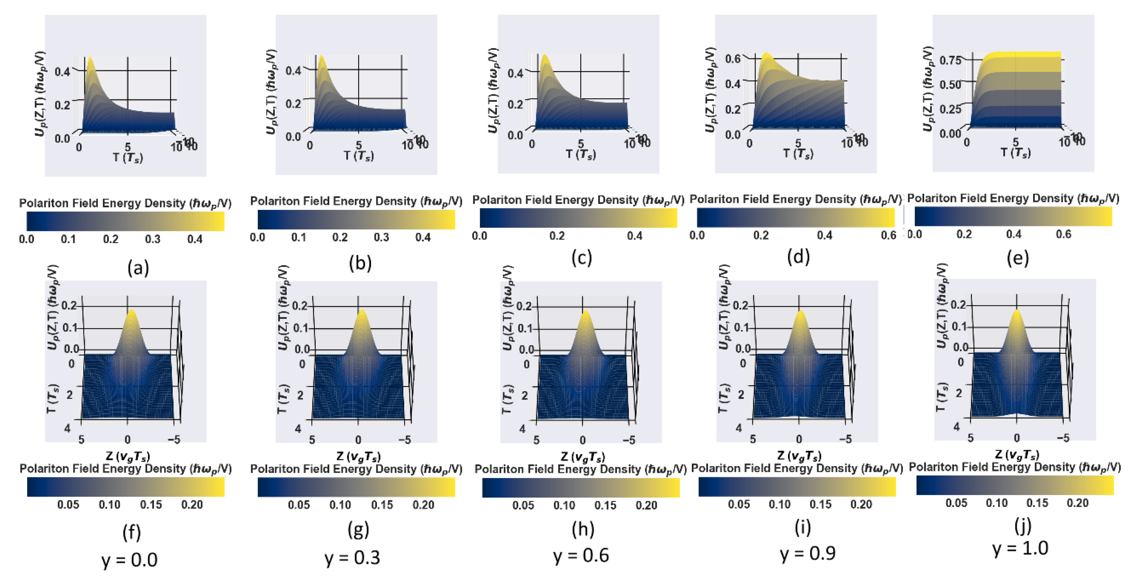
Figure 4.
Plots of FWHM of the pulse broadening against product of the Rabi frequencies of the counter-propagating fields,, showing as we approach perfectly standing wave case, we minimise the pulse broadening, due to the elimination of the atomic diffusion by the cavity modes, generated by the standing wave control laser field.
Figure 4.
Plots of FWHM of the pulse broadening against product of the Rabi frequencies of the counter-propagating fields,, showing as we approach perfectly standing wave case, we minimise the pulse broadening, due to the elimination of the atomic diffusion by the cavity modes, generated by the standing wave control laser field.
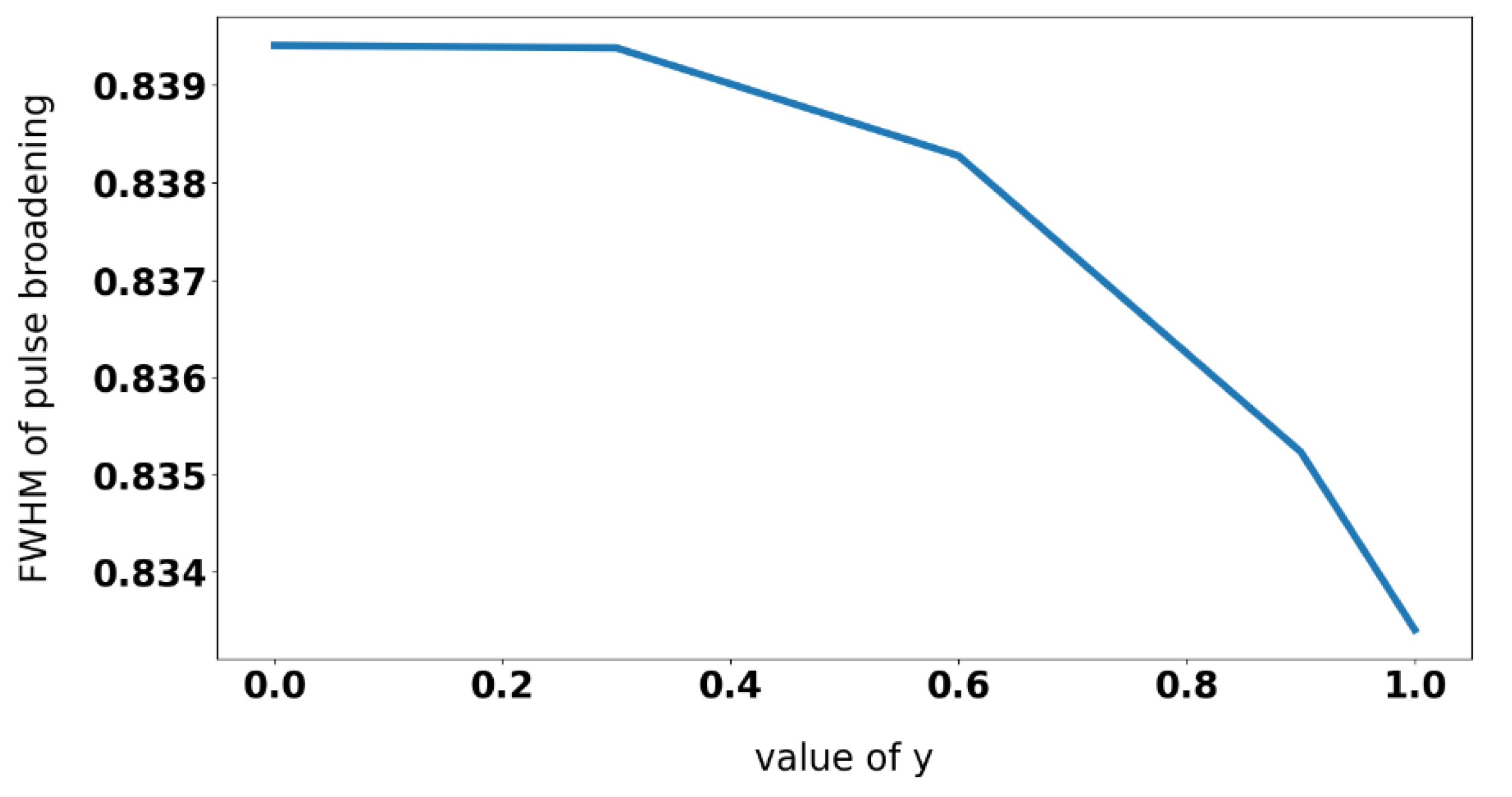
Figure 5.
Plot showing the total storage time of the stored polariton field of the probe pulse for different values of in arbitrary units, based on the time taken for the energy density to fall below 0.01. We have chosen the constants: , time t is in units of , and energy is in units of . Note how standing wave case (y = 1) furnishes us with a prolonged storage time, only limited by the lifetime of the energy levels.
Figure 5.
Plot showing the total storage time of the stored polariton field of the probe pulse for different values of in arbitrary units, based on the time taken for the energy density to fall below 0.01. We have chosen the constants: , time t is in units of , and energy is in units of . Note how standing wave case (y = 1) furnishes us with a prolonged storage time, only limited by the lifetime of the energy levels.
Disclaimer/Publisher’s Note: The statements, opinions and data contained in all publications are solely those of the individual author(s) and contributor(s) and not of MDPI and/or the editor(s). MDPI and/or the editor(s) disclaim responsibility for any injury to people or property resulting from any ideas, methods, instructions or products referred to in the content. |
© 2025 by the authors. Licensee MDPI, Basel, Switzerland. This article is an open access article distributed under the terms and conditions of the Creative Commons Attribution (CC BY) license (http://creativecommons.org/licenses/by/4.0/).
Copyright: This open access article is published under a Creative Commons CC BY 4.0 license, which permit the free download, distribution, and reuse, provided that the author and preprint are cited in any reuse.


