
Submitted:
11 March 2025
Posted:
12 March 2025
You are already at the latest version
Abstract
Attention mechanisms have been widely used to address the common multi-scale challenges in remote sensing imagery for tasks such as object detection and instance segmentation. However, they often require the design of task-specific network architectures tailored to different data targets. To better accommodate objects of varying scales and downstream task requirements, we propose a dynamic search framework based on a Mixture-of-Experts model. In this framework, each module is treated as an expert, and their combinations are flexibly adjusted to ensure that the pyramid structure adapts to the needs of different-scale tasks. Specifically, we design a Scalable Bi-Directional Feature Pyramid Network (SBFPN), which incorporates various hybrid attention mechanisms to dynamically enhance feature fusion across different layers. This approach not only captures long-range dependencies within the image but also suppresses noise and interference from complex backgrounds. The scalable feature pyramid structure we construct utilizes sparse feature fusion within the same layers, while also computing self-attention weights between nodes and retaining or trimming skip connections across layers. We conduct experiments on object detection, instance segmentation, and panoptic segmentation tasks. This structure can be transferred to YOLO-based and R-CNN-based networks, achieving superior detection and segmentation performance. On the Airbus Ship dataset, the mAP for detection and segmentation increased from 71.3% and 62.4% to 82.7% and 71.1%, respectively, demonstrating the effectiveness of our proposed method. Code is available at https://github.com/chaibosong/SAFPN.
Keywords:
remote sensing image
; ship detection and segmentation
; scalable attention feature pyramid
1. Introduction
In recent years, with the rapid development of remote sensing, the shooting cost has gradually decreased, and the resolution has been continuously improved, making it easier to obtain a large number of high-resolution remote sensing images [1]. Instance segmentation is one of the fundamental tasks in the field of intelligent image understanding. It is not only necessary to achieve precise positioning of the spatial location of instances, but also to classify each instance at the pixel level to distinguish different instances.
In order to strengthen the discriminative ability and adapt the network to different scale targets, especially in remote sensing object detection tasks, there are many works that will be improved based on the Feature Pyramid Network (FPN) structure, adding skip connections between different feature layers [2,3,4]. How to design the structure of FPN, how to introduce feature fusion methods to obtain the discriminative high-resolution feature are very worth exploring.
As a widely used technique in deep learning, the attention mechanism plays a crucial role in improving model performance. It adaptively adjusts the model’s focus on different information, effectively allocating computational resources to prioritize more important tasks, thereby enabling efficient processing even with limited resources. In particular, attention mechanisms can effectively alleviate background interference and enhance precise localization of targets in instance segmentation and object detection tasks. Currently, many works [5,6] incorporate various attention modules into structures such as Backbone and FPN. Most attention modules connect basic units in parallel or sequentially, leading to the development of various hybrid attention mechanisms [6,7]. Most tasks require the design of specific network structures based on data scale features, making it a significant challenge to dynamically design the network according to the data scale. Currently, Neural Architecture Search (NAS) algorithms [8] require substantial computational resources. The sparse response characteristic of the Mixture of Experts (MoE) model motivates us to treat different modules as "experts" and use the mixture of experts layers to dynamically design the network structure, thereby improving the model’s adaptability across multiple tasks.
For ship targets of different scales, Guo et al. [9] propose a multi-attention cascaded convolutional neural network (MAC-CNNS), which was an improved YOLOv3 algorithm. Aiming at the problems of missed detection, false detection and low accuracy in small-scale ship target detection, Yu et al. [10] propose an improved YOLOv3 ship target detection algorithm, which fuses features of different scales and outputs enhanced features. In addition, adding the aspect ratio to the loss function makes the loss function more suitable for ship detection. Among these methods, channel and spatial attention modules are introduced to fuse mid-level and high-level semantic features. Although context fusion helps to capture the information of objects at different scales, it cannot represent the relationship between objects in a global view, which is also essential to instance segmentation tasks. And recent methods of ship instance segmentation have to go through a complex data preprocessing stage. Its detection and segmentation accuracy largely depends on the results of the preprocessing stage.
We introduce a self-attention mechanism in the channel and spatial attention modules. For the spatial attention module, we introduce a self-attention mechanism to capture the spatial dependencies between arbitrary locations in the feature map. For the feature at a certain position, it is updated via aggregating features at all positions with weighted summation, where the weight is determined by the feature similarity at the corresponding location. For the channel attention module, we use a similar self-attention mechanism to capture the channel dependencies between any two channel maps, and use the weighted sum of all channel maps to update each channel map. Finally, for the output of the attention module, we adopt a variety of fusion methods to further enhance the feature representation.
We propose an end-to-end method for ship instance segmentation and transfer this method to other tasks. A Scalable Attention Bi-Directional Feature Pyramid structure is proposed, and an attention mechanism is introduced to capture feature dependencies in spatial and channel dimensions, respectively. We design an Attention in experts method based on MoE layers to adaptively build the model structure. Specifically, based on the sparse response results of the MoE gating network, the attention mechanism is either activated or silenced to dynamically design the network structure, and feature fusion methods are incorporated to adapt to tasks with different scales.
It should be noted that in more complex and diverse tasks, our method is more effective and flexible than previous method [9,10,11,12]. Scalable Bi-Directional Feature Pyramid structure based on attention mechanism we propose can express features at different scales with the same semantics, and aims to adaptively integrate multi-scale feature information from a global perspective. Configuring the corresponding hyperparameters such as the number of scalable layers for different downstream tasks to adapt to more tasks.
Our main contributions can be summarized as follows:
- We propose Scalable Bi-Directional Feature Pyramid (SBFPN) with attention mechanism to enhance the discriminant ability of feature representations for instance segmentation. The scalable layers and other hyperparameters are applied for different scale objects, so that the model can be adapted to more downstream tasks.
- We dynamically adjust the network structure through a Mixture of Experts (MoE) model, aiming to enable the model to adaptively select the appropriate structure and accommodate multi-scale tasks.
2. Related Work
2.1. Instance Segmentation
The mainstream implementation schemes for instance segmentation can be divided into two paradigms: detection-based top-down and semantic segmentation-based bottom-up. The detection-based instance segmentation first finds the region where the object is located in the remote sensing image by the method of object detection, performs semantic segmentation from inside of the region, and each segmentation result is output as a different instance. Studies based on such methodologies include an improved Mask R-CNN algorithm [16] propose by Su et al. , which generates bounding boxes and masks for each object instance in remote sensing images while pre-determining the sample points in its Region of Interest(ROIs), thus avoiding accuracy loss. Ran et al. [17] propose an Adaptive Fusion Mask Refinement (AFMR) of instance segmentation network for remote sensing images, AFMR contains two modules, one of which is an adaptive module for unsupervised learning of multi-scale complementary spatial features and the other is a content-aware module for refinement of segmentation masks.
For instance segmentation techniques based on semantic segmentation, the images are first semantically segmented at the pixel level, and then different instances are distinguished by means of clustering and metric learning. Studies based on such methodologies include that Zhang et al. [18] propose an end-to-end multi-instance segmentation network model, which mainly consists of an SEA module and a SCMB branch, where the SEA module contains a fully convolved semantic segmentation branch with additional supervision to reduce the impact of background noise to the segmentation effect, and for the SCMB branch, it extends the original single-mask branch to three and introduces complementary masks of different scales as supervision to make full use of the multi-scale information. Liu et al. [19] brought the self-attention mechanism into the Anchor-free segmentation architecture and propose a Global Contextual Parallel Attention Module (GC-PAM), consisting of a channel self-attention module and a spatial self-attention module, to improve the segmentation accuracy by reassigning weights to the remote sensing image space and channels. Semantic segmentation networks based on deep learning mainly include FCN [20], DeconvNet [21], UNet [22], DeepLab series [23,24,25,26] and other networks. Compared with the method based on semantic segmentation, the method based on detection has higher accuracy. It is only driven by data and does not need to model masks according to different purposes, which reduces human intervention and have stronger generalization ability.
Therefore, this paper is a detection-based instance segmentation method.
2.2. Ship Detection and Segmentation
In the field of ship object segmentation, Feng et al. [27] propose a new framework of SLCMASK-Net, which introduces Sequence Local Context (SLC) to avoid confusion between objects of the same class. Huang et al. propose the OSM-Net network structure [28], using multi-scale features and instance-level masks to achieve anchor-free instance segmentation. Regression was performed simultaneously for each position and angle classified as the target predefined frame. The Adapted RoI-Align method is then used to extract the features of each propose box. Huang et al. propose the SSS-Net network model [29] which is based on PolarMask [30] and has a simple structure and fast prediction speed. It is an end-to-end network model consisting of a backbone network, a feature pyramid, and a dual-task prediction head. One of the tasks is to predict the instance class, center position, and main orientation angle, and the other is to predict the mask. Sun et al. propose a method based on channel-wise attention module [31] for the segmentation of ship instances in cloudy weather: CondInstAtt, which can weaken the interference of fog on the segmentation of ship instances. In addition, in order to solve the problem of lack of data in foggy scenes, which uses an atmospheric scattering model to simulate blurred images in marine scenes. Gao et al. propose an anchor-free instance segmentation method based on centroid distance loss [32], which firstly adopted a lightweight feature extractor and an anchor-free convolutional network to effectively reduce the amount of computation and model complexity.
Second, a dynamic encoder was designed to fully propagate the features and a centroid-based loss function was designed to fully utilize the shape and position relationship between ship objects. Aiming at the problems of insufficient SAR radar remote sensing image data and difficult labeling [33], Zhu et al. propose a SAR ship instance segmentation method based on cross-domain transfer learning. First, the optical image is simulated as a SAR image by the sample transfer module, then the parameters are processed by the knowledge transfer module, to obtain the pre-train model of the instance segmentation task. In addition, the backbone network of this method does not directly use the common deep convolutional neural network, but redesigned ResNet [34] for SAR image characteristics, and propose the Res-Pyramid network, which can extract SAR image features more effectively.
3. Methodology: A Roadmap
In this section, we draw a roadmap from the MaskR-CNN Baseline to our improved model as shown in Figure 1. In order to improve the detection and segmentation effect of small objects, a Bi-Directional Feature Pyramid structure is proposed by making full use of the shallow feature information. We propose a MoE-based approach to model pruning.
3.1. Bi-Directional Feature Pyramid
3.1.1. Bottom-up Path Argumentation
Low-level features carry more location information, which is particularly useful for detection and segmentation tasks. What FPN does is to retroactively transmit high-level information to maximize the use of the semantic information of the feature map. In PANet [35], Liu et al. introduced a bottom-up path on this basis, which makes it easier to transfer low-level information to the top of high-level and improves the utilization of low-level information.
The bottom-up path constitutes a Bi-directional feature fusion with the top-down path in the original feature pyramid. We use ResNet and FPN structures to obtain four feature maps with different resolutions: {C2, C3, C4, C5}, and the output feature maps through the original feature pyramid are:{P2, P3, P4, P5}. As shown in the Figure 2, the Bi-Directional Feature Pyramid outputs feature map{N2, N3, N4, N5}, which is obtained by the following steps: top-down expansion path from N2 to N5, where N2 is of the same size as P2. After downsampling the feature map, the result is summed with Pi+1. And then the superimposed shadow of fusion is eliminated by a convolutional layer with a convolutional kernel size of 3 × 3 to generate a new feature map {N2, N3, N4, N5}.
3.1.2. Sparse Feature Fusion (Skip Connection)
In this paper, it is found that the detection and segmentation accuracy of large objects decreases after only adding the bottom-up path. To solve this problem, this paper proposes a feature fusion approach: when the input and output feature maps of the Feature Pyramid are at the same level of resolution, we add a Skip Connection from the input to the output to fuse more features. The red solid line in Figure 3 shows the added Skip Connections. With the addition of skip connections to the Bi-Directional Feature Pyramid, only the feature fusion process of the bottom-up path has changed.
As shown in the Figure 4, the Skip Connection feature fusion process is implemented by the following steps: high-resolution feature map and low-resolution feature map and input feature map to generate a new feature map .
Specifically, the number of channels becomes 256, after passes through a convolutional layer with a convolutional kernel size of . is reduced to half of the original width and height of the feature map through a downsampling operation, and is added element by element with . The result of the fusion is then passed through a convolutional layer with a kernel size of to obtain the output of the feature pyramid: . The process is shown:
It should be noted that the input feature maps and of the same resolution size are added element by element. The fusion result is passed through a convolutional layer with a convolutional kernel size of , and the output result is .
3.2. Attention Mechanism
3.2.1. Basic Attention Unit
-
Spatial Attention (SA)The spatial attention mechanism treats spatial convolution features differently, assigning more weights to target feature regions and devoting more “attention” to target regions. It assigns small weights to background and noise regions in order to achieve “suppression” of background and noise distractors. The spatial attention module is designed as follows in Figure 5(a). Given an input feature map , we use a convolution to fuse and compress the feature map F into a feature map with one channel, and then activate it by a Sigmoid function to generate a spatial attention mask.
-
Channel-wise Attention (CA)In convolutional neural network, the features of different channels will respond to different semantic information. As shown in Figure 5(b), using the channel attention mechanism, channels with higher target response are assigned larger weights, and channels with lower target response are assigned smaller weights, so that the network pays more attention to those channels with higher response. Our designed channel-wise attention module is implemented as follows.Given the input feature map , we perform global average pooling and maximum pooling operations for each feature channel of the feature map F to generate the fused feature maps . The output results are summed up using a convolution kernel of size to perform convolution operations on the feature maps , respectively. We multiply the feature map F with the channel attention map element by element and add the result with the feature map F. The final output result of the channel-wise attention module is obtained, and the weight assignment for each channel is achieved.
-
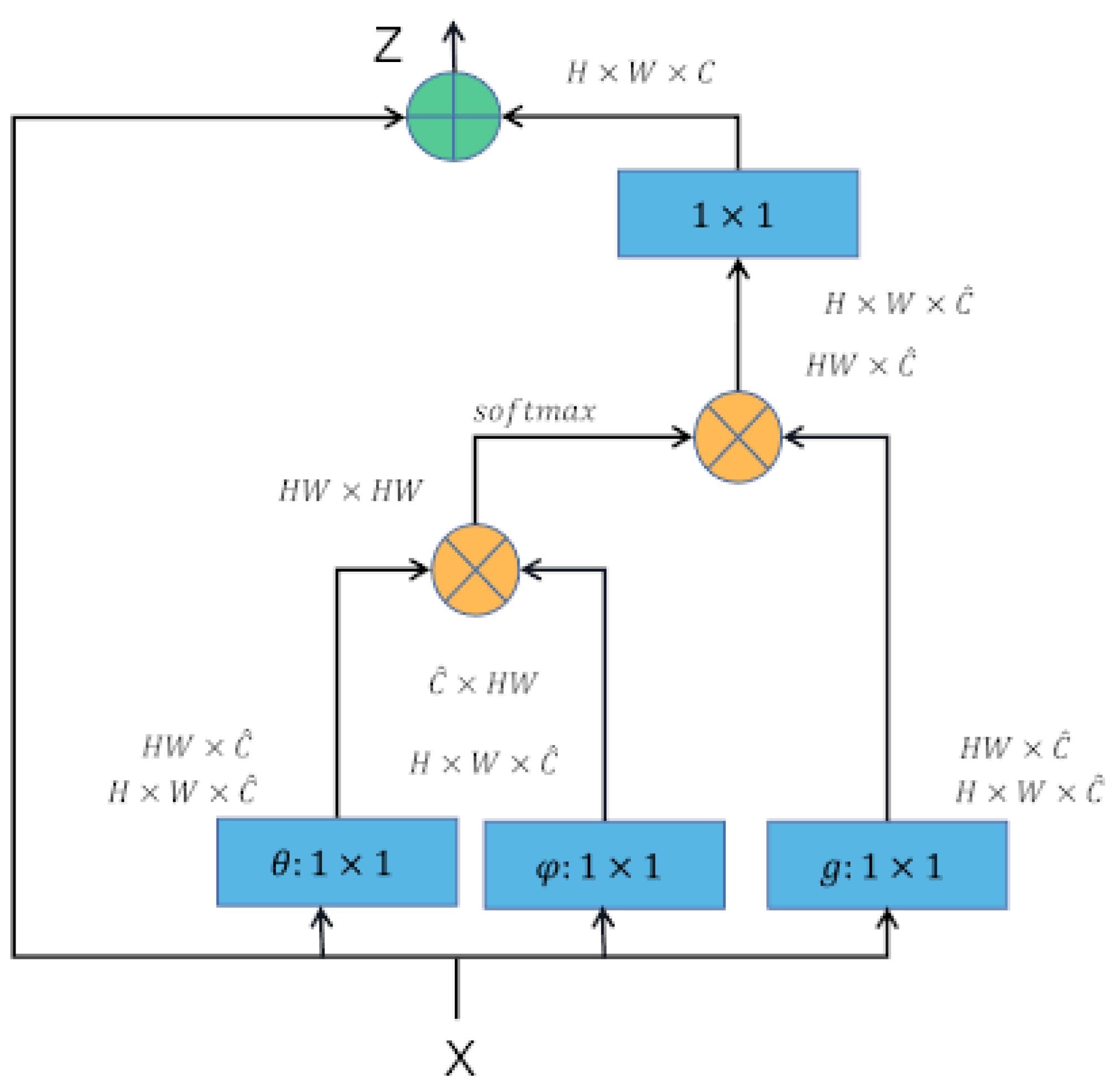
Non-local Attention (NA)The self-attention mechanism was first applied in the field of natural language processing, and later in the novel Non-local network proposed by Wang et al. which applied the self-attention mechanism to computer vision tasks [36]. Non-local can be used as a component to combine with other network structures. The whole process is divided into four steps:
- Convolution operation is performed on the output feature map X using three convolution kernels of size to achieve a linear mapping to compress the number of channels and obtain features.
- Do matrix multiplication operation on and , that is, calculate the autocorrelation in the features.
- Do softmax operation on the autocorrelation features to get the weights from 0 to 1, that is, the self-attentive coefficients.
- Perform matrix multiplication operation on the self-attentive coefficients and g, and later do residual operation with the feature map X to get the output of Non-local block. The formula of Non-Local is defined as follows:
Figure 5.
Illustration of Channel Attention (CA) and Spatial Attention (SA).
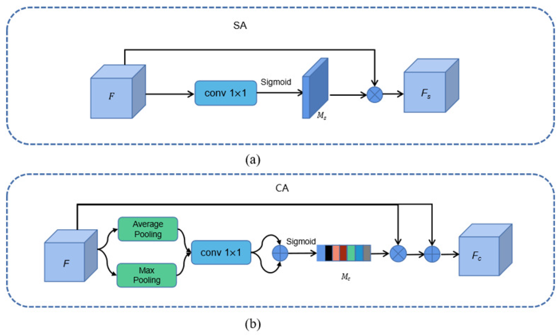
Figure 6.
Schematic diagram of model pruning method based on self-attention.
3.2.2. Mixture-of-Experts (MoE) Attention Layer
Each expert module has an associated gating weight , which is computed by the router gate. Suppose there are n expert modules, and the input data x passes through the router gate to compute the activation weights for each expert. The output of the router gate can be expressed as:
where represents the activation probability of the expert . This value is calculated by the router gate network based on the input x, indicating the activation degree of that expert module. Each expert computes its output based on its corresponding weight . Suppose the output of each expert is , then the final output y is the weighted sum of all the experts’ outputs.
Here, represents the output of expert for the input x, and is the weight of the expert, determining the contribution of that expert to the final output. To ensure the efficiency of the model, we set a threshold to prune out low-weight expert modules. If is less than the threshold , the corresponding expert module will be pruned. This means that if the gating weight of an expert is below the threshold , that expert module will not contribute to the final output computation, thus achieving pruning.
In object detection and semantic segmentation tasks, we utilize the principles of the MoE model, combining attention mechanisms with expert models to improve model performance and achieve adaptive network design. Specifically, each attention module can be regarded as an expert, and through the router gate, we dynamically select and combine different experts to optimize the model’s structure and performance. As shown in Figure 7, if there are n basic attention units as expert modules waiting for us to use, we can dynamically select these experts using the router gate mechanism. During training, the router gate computes the corresponding attention weight for each module based on its input data and determines which experts should be activated. Specifically, the router gate calculates the weight for each expert and decides whether to activate the expert module based on these weights. If the weight of an expert module exceeds a set threshold, the expert is activated; if it is below the threshold, the expert module is pruned, thus optimizing computation and reducing redundancy.
We adopt a dynamic connection method, where attention expert modules are connected both in series and in parallel, and the router gate mechanism determines whether each module should be activated. As shown in Figure 8, residual connections between modules are combined with the self-attention mechanism, ensuring that the network can dynamically weigh different paths. The router gate mechanism assigns a weight to each path based on the current input data, enabling the model to flexibly select and combine expert modules according to the specific task and data requirements. Subsequently, the network prunes paths with low weights, thereby improving efficiency.
3.2.3. Hybrid Attention Module
This section will introduce the implementation details of three hybrid attention modules with the highest detection and segmentation performance based on Mixture-of-Experts Attention Layer to .
This section will delve into the implementation details of three hybrid attention modules, which achieve the highest performance in detection and segmentation tasks, based on the MoE Attention Layer.
-
Channel-wise and Non-local and Spatial Attention Module (CA-NA-SA)The structure of the Channel-wise and Non-local and Spatial Attention module (CA-NA-SA) is demonstrated. The feature map F is first passed through the channel-wise attention module to obtain the channel-level attentional features , and then input to the Non-local Attention module. It should be noted that Non-local Attention computes the relational vector with the same size of output and output feature maps, while there is an identity mapping from input to output. Therefore, the Non-local Attention module can be embedded as a generic module in other modules. Feeding into the spatial attention module to obtain the Channel Attention - Non-local Attention - Spatial Attention Module .
-
Channel-wise and Spatial Attention Module (CA-SA)As shown in Figure 9(a), the structure of the Channel-wise and Spatial Attention (CA-SA) Module is demonstrated. The feature map F is first passed through the channel attention module to obtain the channel-level attentional features , and then is input to the spatial attention module to obtain the final channel-spatial attentional feature , which is calculated as follows.Where S denotes the spatial attention module computation process and C denotes the channel attention module computation process.
-
Parallel [Channel-wise and Spatial] Attention Module ([CA-SA])As shown in Figure 9(b), the structure of the parallel [channel-wise and spatial] attention module is demonstrated, and its implementation process is more different from the first three types of attention modules in series connection. First, a three-dimensional attentional map is inferred from the input feature map . And then is multiplied element by element with the feature map F. The output result is summed up with the original input feature map F, that is, the output of the Parallel [Channel-wise and Spatial] Attention Module is obtained, and its calculation procedure is as in Eq. (4), where ⊙ denotes element-by-element multiplication.The input feature map is processed through the spatial attention branch and the channel attention branch to obtain the spatial attention map and the channel attention map , respectively, where the spatial attention and channel attention branches follow the process implemented in the Spatial Attention Module and the Channel Attention Module in this paper. After extending the two attention maps to , they are fused by adding each other element by element, and the fusion result is processed by a Sigmoid activation function to obtain an with output values between [0,1], which is calculated as in formula 6. In which, denotes the Sigmoid Function calculated by.
3.3. FPN and Bottom-up Structures with Attention Module
In this section, we attempt to add the attention in attention module to the FPN and bottom-up structures, respectively, so as to make best and different combinations of the attention modules, in order to improve the network’s feature extraction.
Figure 10.
(a) FPN with attention module. (b) Bottom-up structure with attention module. 17 different types of Attention Modules (AM): Including attention module and hybrid attention module.
Figure 10.
(a) FPN with attention module. (b) Bottom-up structure with attention module. 17 different types of Attention Modules (AM): Including attention module and hybrid attention module.
3.3.1. FPN with Attention Module (FPN-AM)
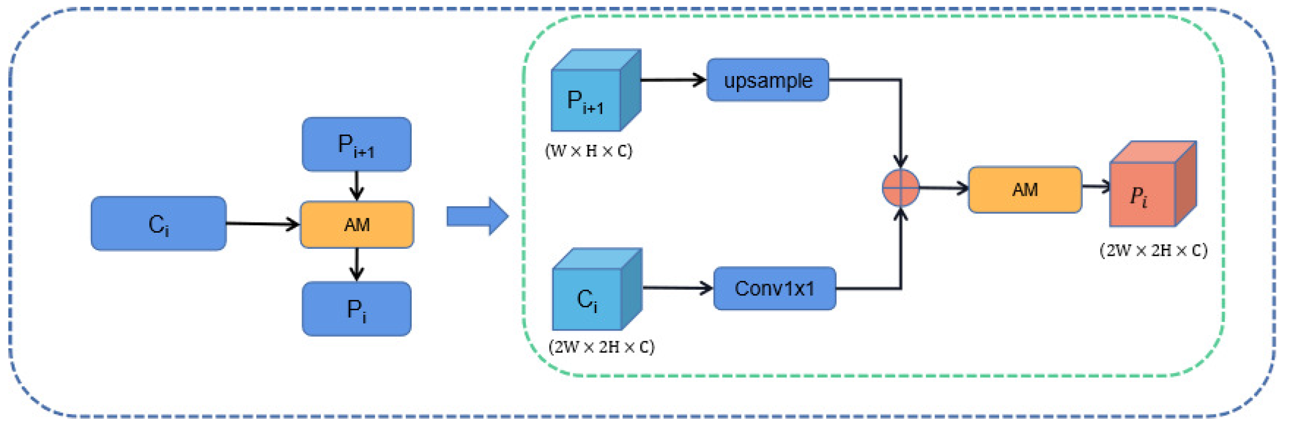
We first tried to introduce an attention mechanism in the FPN structure, called FPN-AM, which is shown in Figure 11. We used ResNet to obtain four feature maps with different resolutions: . In the horizontal connection of the original FPN structure, the feature layer is upsampled and then subjected to an element-by-element summation operation with of channel number 256. The FPN structure with the attention mechanism is to replace the horizontal connections in the original FPN structure using the attention module designed in the previous section, which is implemented as shown in Fig.
The output feature maps of the FPN-AM structure are obtained by combining the FPN with the attention module. It’s calculated as follows. The feature map is obtained by convolutional layers with a channel number of 256 and a convolutional kernel size of size . Upsampling operations with multiplicity 2 are performed for , respectively, and the results are summed element by element with the corresponding feature maps () for feature fusion to generate feature maps . The feature map is fed into the selected attention module (one of the 17 attention modules designed in the previous section) to obtain . Then the FPN-AM structure obtains the attentional feature pyramid which is fed into the Mask-R-CNN follow-up network.
3.3.2. Bottom-up with Attention Module (Bottom-up-AM)
Then, we tried to introduce an attention mechanism in the bottom-up path, called Bottom-up-AM, The structure shown in the Figure 10(b) and Figure 12, which is similar to the FPN-AM structure. We denote the input feature layer as N2 in, N3 in, N4 in, N5 in, and the feature map obtained from the bottom-up path as .
As the Figure 12 shows the specific implementation details, the output feature maps , , , are obtained by the following steps: a downsampling operation is performed on the high-resolution feature map to obtain the feature map , whose height and width are half of the original. The feature map is added element by element with the feature maps and , and the fused result is subjected to a convolution operation with a convolution kernel size of to obtain the fused feature map . Then the fused feature map is later sent to the selected attention module (one of the 17 attention modules designed in the previous section) to obtain the attention feature map . The output of the feature fusion layer , is also the input of the next feature fusion layer.
We also tried to introduce the attention mechanism into the FPN structure and the Bottom-up structure at the same time, and the implementation steps are similar to those in the previous section. There’s no need to elaborate.
3.4. Scalable Bi-Directional Attention Feature Pyramid
In order to make the extracted features more highly semantic information and enhance the feature extraction, we stack this Two-Way Attention Feature Pyramid structure as a basic feature fusion layer, so that the model can meet various resource condition constraints and achieve a more advanced feature fusion method. The output of the feature fusion layer , which is also the input of the next feature fusion layer, connects multiple Bi-Directional Attention Feature Pyramid structures in series to achieve its scalability. An improved Mask R-CNN model structure based on a Scalable Bi-Directional Attention Feature Pyramid structure is illustrated in Figure 13. Using for the stacking of feature fusion layers, the fusion of up-sampled and down-sampled features can be continuously performed. After stacking the enhanced feature extraction network, effective feature layers with high semantic information are obtained, and these features are integrated and utilized to obtain prediction results.
We can also search for the best Bi-Directional FPN structure for this task based on self-attention between FPN node connections. However, under limited computing resources, we only verified the addition of skip connections and scalable structures, and calculated the self-attention value of its nodes. The experimental results show that the self-attention results between the expansion layer nodes are higher than the threshold we set, and should be kept and will not be pruned. This shows that the skip connection method and scalable structure we designed is an effective feature fusion method.
3.5. Other Tricks
In order to explore the limit that the model can achieve, further improve the performance of the model, and make the model have better accuracy and generalization ability, we have made a series of attempts.
3.5.1. Adjustment for Backbone
-
Group ConvolutionIn ResNeXt [37], Saining Xie et al. introduced Group Convolution to the residual network to improve the accuracy of the model and enhance the feature representation of the model without significantly increasing the number of parameters. Inspired by ResNeXt, we adopted a similar approach by replacing the convolutional structure of size in each Stage of the original ResNet-101 network with a grouped convolutional structure and setting groups of all grouped convolutions to 32.
-
Activation FunctionThe performance of the ReLU activation function decreases as network layers deepen. The Swish function has lower bound, smooth, and non-monotonic properties. The Swish activation function inherits advantages of the ReLU activation function and does not have the gradient disappearance problem, and performs better in deep networks. We try to replace the ReLU activation function in the residual network with the Swish activation function.The Swish activation function is formulated as follows.where is a constant or trainable parameter, and the value of is set to 1 in the paper.
3.5.2. Training Techniques
In addition to the network structure design, the training strategy also has a significant impact on the model performance. In this paper, a training strategy similar to DeiT [38] and Swin Transformer [39] is used. The maximum number of iterations was increased from the initial 350,000 to 500,000. We use the AdamW [40] optimizer, using data augmentation techniques such as Mixup [41] and regularization methods such as Label Smoothing [42]. It has been shown [42] that the two-stage algorithm can be used for data augmentation without random geometric transformations in the training phase. We use Synchronized Batch Normalization [43] to solve the multiple GPU cross-card synchronization problem. For the learning rate setting, we borrowed the training strategy of YOLO-v3 [44], and in the first 2000 iterations, we use warm-up [45] to gradually increase the learning rate from 0 to the preset base learning rate, and subsequent iterations with the cosine [45] strategy, which is conducive to the stability of the training process. We use Apex-based hybrid precision [46] training to accelerate the training with as little loss of precision as possible.
3.5.3. Loss Function
In this section, we introduce the DIoU Loss loss function for the problem of ignoring the interrelationship between coordinate points using the Smooth loss function in Mask R-CNN networks.
1) Whether it is feasible to minimize the normalized distance between the prediction frame and the target frame to achieve faster convergence.
2) How to make the regression more accurate and faster when there is overlap or even inclusion with the target box.
Based on these two problems, Zhaohui Zheng et al. [47] proposed DIoU Loss, which converges faster relative to GIoU Loss and takes into account the overlap area and the distance of the centroid. The DIoU takes values in the range . The DIoU Loss function is defined as:
4. Experimental Results on Airbus Ship Dataset
This section depicts the experimental process of step-by-step model tuning for our roadmap. The Airbus Ship dataset is used in a large number of experiments.
We focus on the common objects and use the improvement of average detection and segmentation accuracy as the judging metric. In our roadmap, the accuracy of large, medium, and small targets has been improved to varying degrees.
4.1. Airbus Ship Dataset
In this paper, we use the dataset of Kaggle remote sensing image detection segmentation competition (Airbus Ship), which contains remote sensing images of ships in different regions and various scenes, and the pixel size of the images are all . There are about 150,000 images in this dataset, but most of the images do not contain ships. In the experiment, the images containing ships are screened and some images with poor image quality are removed. Finally, 48,000 images are left. From them, 3,500 images are randomly selected as the test set, and the remaining images are used as the training set. The dataset is encoded in RLE format for the semantic segmentation task in an annotation manner. In order to be applicable to the object detection and instance segmentation tasks in this paper, we transformed it into the COCO annotation format [48].
4.2. Implementation Details and Results
This section measures and evaluates the performance of the model using the AP-related metrics of the COCO evaluation criteria, which incorporate multiple IoU thresholds (AP, AP50, AP75) and multiple object scales (APs, APm, APL). In the RPN structure of Mask R-CNN, an area-scale Anchor is assigned to each level feature, corresponding to five levels with five scales assigned , and the aspect ratio of each level Anchor is .
The PyTorch version 1.1.0 was used in our experiments and the basic code used was Facebook Research’s Mask R-CNN Benchmark [43]. In our experiments, we use the pre-trained ResNet-101 model for initialization. The GPUs used in our experiment were two Nvidia GeForce GTX 4090 with 24 GB memory.
The proposed method is an improved model based on the Mask R-CNN network, so the experimental results of the Mask R-CNN network are selected as the baseline data. In order to enhance the persuasive power of the experimental data, all experimental parameter settings keep unchanged.
4.2.1. Experimental Analysis of Scalable Bi-Directional Feature Pyramid Structure
Table 1 shows that by adding only the bottom-up path, the accuracy AP of ship detection and segmentation reaches 73.9% and 63.9%, which are improved by 2.6% and 2.5%, respectively, where the detection and segmentation accuracy APs of small target ships improves from 63.2% and 50.8% to 64.8% and 52.9%, which are improved by 1.6% and 2.1%, respectively. After adding the skip connection from input to output, the accuracy AP of ship detection and segmentation reaches 74.6% and 65.7%, respectively. They have improved by 0.7 percent and 0.8 percent, respectively, when compared to before the addition. The large target ship detection and segmentation accuracy APL improves significantly from 87.0% and 84.3% to 88.8% and 85.9%, which are improved by 1.8% and 1.6%, respectively, thus verifying the feasibility of our proposed feature fusion approach.
In the paper, the proposed bidirectional feature pyramid structure is stacked as one feature fusion layer to achieve its scalability. Table 1 demonstrates the effects of different feature fusion layer stacking times a on detection and segmentation accuracy. In this paper, experiments are conducted for a taking values 1, 2, 3, and 4, respectively. When , the model detection and segmentation accuracy AP reaches 76.4% and 66.4%, respectively, and has a fast fitting speed. Repeated stacking of feature fusion layers enables more advanced feature fusion, which improves the performance of the model. It is an effective way of model expansion.
4.2.2. Experimental Analysis of the Attention Module
In this section, based on the previous Scalable Bi-Directional Feature Pyramid Structure, the 17 attention modules designed in the previous section are added to the FPN and bottom-up structures, respectively, and the number of feature fusion layer stacking a is set to 2. Table 2 and Tables 7 and 8 in Appendix show the experimental results of introducing the attention mechanism in the FPN and bottom-up structures, respectively. The symbolic representation of the attention module is shown in Tables 16 and 17.
The experimental results show that the order of the attention modules in series does not have a significant effect on the model detection and segmentation accuracy AP, within 0.8%. We introduce four attention modules (CA-SA, CA-NA-SA, NA, SA-NA) with the best performance in the FPN structure above for further experiments.
4.2.3. Other Experimental Analysis
This section adjusts the network backbone structure, introduces the DIoU loss function, and optimizes the training strategy to further improve the model detection and segmentation accuracy.
Table 3, Group Convolution and Swish activation function are introduced in the backbone part. The introduction of grouped convolution and Swish activation function improves the detection and segmentation accuracy of the model from 79% and 68.2% to 81.7% and 70.5%, which enhances the feature representation capability of the model. Recent studies have shown that the DIoU loss function converges faster and has higher accuracy in target detection and instance segmentation tasks. The introduction of DIoU loss function does deal with the problems of that Smooth, IoU Loss and (L1) GIoU Loss cannot optimize the situation and degradation to some extent, but it does not improve for segmentation and detection accuracy in the experiment. We believe that DIoU Loss is insensitive to the Multi-Stage R-CNN networks (such as this paper based on Mask R-CNN). We tried to increase the weight of DIoU Loss in the loss calculation, but did not achieve good results.
We use the training strategy from the previous section. There is a further improvement in detection and segmentation accuracy, from 81.7% and 70.5% to 82.7% and 71.1%. This means that a good training strategy can squeeze the extreme accuracy of the model.
4.3. Comparison with Other Methods
In this section, the method in the paper is compared with Mask R-CNN baseline model, PANet [35], Mask Scoring R-CNN, Cascade Mask R-CNN, and Mask R-CNN(using SoftNMS) [49] methodologies on Airbus Ship dataset for detection segmentation effect respectively. To make the experimental results more convincing, we used the same number of iterations and learning rate strategies.
Reference [49], Mask R-CNN+ S-NMS replaces the NMS in Mask R-CNN with Soft-NMS and achieves better results in ship detection and segmentation tasks. Mask Scoring R-CNN [11] is an improved version of Mask R-CNN. Mask Scoring R-CNN proposes a method to score the "instance segmentation hypothesis" of the algorithm. It outperforms Mask R-CNN on the image instance segmentation task for the COCO dataset. The bottom-up path structure in our proposed Bi-Directional Feature Pyramid Structure is inspired by PANet, which is also a modified version of Mask R-CNN. In the experiments of this paper, PANet improves the ship detection and segmentation accuracy by 1.3% and 0.8%. Cascade Mask R-CNN [50] uses different IoU thresholds to improve the proposal quality by multiple regressions, thus improving the detection quality. Cascade Mask R-CNN has a high accuracy of 96.1% and 88.6% and 95.0% and 86.8% for detection and segmentation of large and medium ship targets.

Table 4.
Detection/ Segmentation Accuracy of Different Methods.
| Method | AP | |||||
| Mask R-CNN | 71.3/ 62.4 | 94.6/90.8 | 81.7/71.8 | 63.2/ 50.8 | 86.6/ 79.1 | 87.2/ 84.1 |
| PANet [35] | 72.6/ 63.2 | 95.1/82.3 | 80.4/ 68.5 | 63.0/ 49.4 | 89.4/ 79.5 | 91.4/ 84.9 |
| Mask Scoring R-CNN [11] | 65.8/ 56.2 | 93.5/ 89.7 | 72.5/ 60.2 | 54.4/ 42.0 | 85.3/ 78.2 | 88.7/ 85.2 |
| Mask R-CNN+ S-NMS [49] | 66.5/ 56.2 | 88.6/89.7 | 75.3/ 67.6 | 55.4/ 46.5 | 85.7/ 79.4 | 88.3/ 85.2 |
| Cascade Mask R-CNN [50] | 72.9/ 65.2 | 86.1/84.9 | 77.3/ 73.4 | 61.0/ 53.0 | 95.0/ 86.8 | 96.1/ 88.6 |
| (ours) | 82.7/ 71.1 | 97.4/95.3 | 90.2/80.3 | 76.9/ 61.8 | 93.9/86.9 | 93.4/ 89.3 |
Table 5.
Detection/ Segmentation Accuracy of Different Models on Is AID Dataset.
| Method | AP | |||||
| Mask R-CNN | 37.7/ 36.5 | 63.7/ 59.1 | 46.0/ 37.5 | 26.9/20.9 | 48.7/42.5 | 55.1/ 50.5 |
| PANet [35] | 42.6/ 34.2 | 64.2/ 59.1 | 46.4/ 37.9 | 27.2/20.9 | 48.8/42.4 | 55.1/ 51.4 |
| PANet+ [14] | 46.3/38.5 | 64.3/ 59.5 | 45.9/ 38.4 | 26.5/21.2 | 50.7/42.7 | 56.8/ 52.5 |
| Mask Scoring R-CNN [11] | 41.7/35.5 | 63.5/ 58.8 | 46.1/ 37.7 | 26.9/20.9 | 48.3/42.4 | 54.8/ 51.4 |
| Cascade Mask R-CNN [50] | 43.2/ 37.1 | 63.5/ 59.6 | 45.7/ 37.2 | 26.8/ 20.6 | 50.0/43.6 | 55.9/ 52.4 |
| (ours) | 47.3/40.7 | 64.2/ 60.2 | 48.3/ 39.2 | 28.7/21.1 | 51.2/44.3 | 57.5/ 51.9 |
Figure 14[a]-[h] show the detection and segmentation performance of different models under different noise interference scenes (normal scene, near-shore scene, and cloud scene), respectively. Compared with other models, the detection and segmentation performance APs of the method in this paper is significantly improved for ships of various sizes (small, medium, and large), especially small ships (from 63.2% and 50.8% to 76.9% and 61.8% compared to the baseline segmentation accuracy), and the best performance is achieved for ship detection and segmentation in different scenarios. Intuitively, the method in this paper has a smaller proportion of missed detection in different scenes and has better category object segmentation and detection accuracy. Compared with the baseline network Mask R-CNN detection and segmentation accuracy is improved by 11.4% and 8.7%, which verifies the effectiveness of the roadmap in this paper.
Table 6.
The Segmentation Results on Cityscape Dataset Test Set and Validation Set.
| Method | Extra Data | Extra Data | ||
| Mask R-CNN | × | 31.5 | × | 26.2 |
| PANet [35] | × | 36.5 | × | 31.8 |
| PANet | - | - | ✓ | 36.4 |
| Panoptic-DeepLab [51] | ✓ | 38.8 | ✓ | 39.0 |
| Panoptic-DeepLab | × | 35.3 | × | 34.6 |
| Panoptic-FPN [52] | × | 33.0 | - | - |
| GAIS-Net [53] | ✓ | 37.1 | × | 32.5 |
| AUNet [54] | × | 34.4 | - | - |
| AdaptIS [55] | × | 36.3 | × | 32.5 |
| UPSNet [56] | 37.8 | ✓ | 33.0 | |
| UPSNet | × | 33.3 | - | - |
| (ours) | × | 38.6 | × | 36.7 |
4.4. Ablation Studies
The experimental results are shown in Tables 12–15 in the Appendix. Our roadmap is a process of continuous ablation experiments, so some ablation experiments are added to this to analyze the contribution of each method in the roadmap to the accuracy improvement.
The effectiveness of the attention modules is analyzed in Table 12. The best performing attention modules (CA-SA, CA-NA-SA, NA, SA-NA) are introduced in the FPN structure of the Mask R-CNN base network. There is a 3.0% and 2.0% improvement in detection and segmentation accuracy compared to the highest (CA-SA) of the Mask R-CNN network.
Referring to Table 1, Table 2, 14 and 15, comparing (Mask R-CNN+ B) and (Mask R-CNN+B+=[1,2,3,4]), the highest detection and segmentation accuracy (= 2) is improved by 1.2% and 2.1%. Comparing the (Mask R-CNN+B-AM+=[1,2,3,4]), (Mask R-CNN+B+SC+=[1,2,3,4]) and (Mask R-CNN+B-AM+SC+=[1,2,3,4]) three sets of experiments, the stacking of (Mask R-CNN+B-AM) compared to (Mask R-CNN+B+SC) feature fusion layers is more significant for accuracy improvement when CA-SA attention units are selected for the attention module AM. This shows that the stacking of feature fusion layers with different modules added to them, the contribution of different modules to the accuracy improvement during the stacking process is different. When = 3 or 4, the detection and segmentation accuracy of this task does not improve further and introduces additional number of parameters. Many experiments also confirm the superiority of the method chosen for our roadmap.
5. Experimental Results on Other Tasks
5.1. Cityscape Dataset
The Cityscape dataset is currently recognized as one of the most authoritative and professional datasets in the field of image segmentation. The dataset can be used in tasks such as semantic segmentation, instance segmentation, and panoramic segmentation. The dataset contains pixel-level annotations for 19 categories, of which 8 are instance categories (bicycle, bus, person, train, truck, motorcycle, car, and rider) and 11 are stuff categories. The dataset consists of 5000 finely labeled images and 20000 coarsely labeled images. There are fine and coarse evaluation criteria, and only fine labeling is used in this experiment. The resolution size of these images is . 2975 of the finely labeled images are used as the training set, 1525 as the test set, and 500 as the validation set.
5.2. Results on Cityscape Dataset
5.3. iSAID Dataset
The iSAID dataset is a large-scale densely annotated air-borne remote sensing dataset based on the re-annotation of the DOTA 1.0 dataset. This dataset can be used for object detection, semantic segmentation, and instance segmentation tasks, and contains 2806 high-resolution images with a total of 655,451 instance objects in 15 categories. 1/6 of the images were used as the validation set, 1/3 as the test set, and 1/2 as the training set. The 15 categories are: Plane, baseball-diamond, bridge, ground-track-field, Small-vehicle, Large-vehicle, ship, Tennis-court, Basketball-court, Storage-tank, Soccer-ball-field, roundabout, harbor, Swimming-pool, helicopter. The image resolution size ranges from 800 to 13000 pixels. In this paper, we use the preprocessing benchmark officially provided by the iSAID dataset to crop the image to pixels size for training and prediction.
As shown in Figure 15, the experimental environment in this section is the same as the previous section, the maximum number of iterations in training is set to 150,000, and the performance of instance segmentation model is evaluated by the evaluation criterion Mask AP. This experiment uses (Mask R-CNN+B-AM+SC+). The finely labeled images are used for training and no additional data is introduced. Good results are obtained on the test and validation sets. In Table 6, on the validation set, again without using additional training data, our results are 5% higher than UPSNet [56] and 3% higher than Panoptic-DeepLab [51]. On the test set, without using additional training data, our results are 2.1% higher than Panoptic-DeepLab and 4.2% higher than AdaptIS [55].
5.4. Results on iSAID Dataset
The experimental environment in this section is the same as the previous section, and the maximum number of model training iterations is set to 350,000. We process the data according to the requirements of the official website, and crop the training and test images to a size of 800×800. We use the AP-related metrics in the COCO evaluation criteria to measure and evaluate the performance of the model against Mask R-CNN, PANet, PANet+, Mask Scoring R-CNN, and Cascade Mask R-CNN, respectively. The experimental results are shown in Tables 5, 9, and 10. Our AP metrics for detection and segmentation accuracy are 2.0% and 1.7% higher than PANet, and 3.2% and 2.5% higher than Mask R-CNN, respectively. The proportion of missed detection in this study is reduced, and category object segmentation and detection accuracy are better, as demonstrated in the detection and segmentation results of ships, small-vehicles, and large-vehicles in Figure 16.
6. Conclusion
In this paper, we propose an end-to-end method for remote sensing image detection and segmentation, and design a Scalable Bi-Directional Feature Pyramid (SBFPN) Structure based on attention units to improve the model’s ability to learn global contextual information. It efficiently fuses low-level features in shallow networks and high-level features in deep networks, and enhances the network feature extraction capability. By combining attention modules, we explore methods to suppress noise in remote sensing images and improve the detection and segmentation of large and small objects. Compared with the baseline model, it significantly improves the detection and segmentation accuracy, and achieves higher accuracy on the publicly available datasets Cityscape and iSAID datasets to further validate the generalization ability of the model.
The whole set of methods we propose can be transferred to common object detection, semantic segmentation, panorama segmentation tasks, that is, adjusting the FPN structure of the original network, adding our proposed Scalable Attention Bi-Directional Feature Pyramid to the basic network, such as the YOLO series of networks, R-CNN series network, SSD series network, make the network have stronger feature extraction ability. By adjusting the number of scalable layers, training strategies, etc., the model can be adapted to the needs of different scenarios, and corresponding hyperparameters can be formulated for specific downstream tasks. The method in this paper is based on the fact that the attention mechanism is unsupervised, and we try to supervise the attention mechanism based on the annotation information in future work to further improve the feature extraction capability of the network. We will also try to compress the model by knowledge distillation, pruning, and other methods to improve the detection speed.
Acknowledgments
This work was funded by the Scientific Research Fund of Chengdu University of Information Technology (Grant No. KYTZ2023044), National Science and Technology Major Project (Y2022-V-0002-0028) and National Science and Technology Major Project (J2019-V-0003-0094).
References
- Li, K.; Wan, G.; Cheng, G.; Meng, L.; Han, J. Object detection in optical remote sensing images: A survey and a new benchmark. ISPRS journal of photogrammetry and remote sensing 2020, 159, 296–307. [Google Scholar]
- Pi, Z.; Shao, Y.; Gao, C.; Sang, N. Instance-based feature pyramid for visual object tracking. IEEE Transactions on Circuits and Systems for Video Technology 2021, 32, 3774–3787. [Google Scholar]
- Pi, Z.; Shao, Y.; Gao, C.; Sang, N. Instance-based feature pyramid for visual object tracking. IEEE Transactions on Circuits and Systems for Video Technology 2021, 32, 3774–3787. [Google Scholar]
- Sun, Y.; Su, L.; Luo, Y.; Meng, H.; Zhang, Z.; Zhang, W.; Yuan, S. IRDCLNet: Instance segmentation of ship images based on interference reduction and dynamic contour learning in foggy scenes. IEEE Transactions on Circuits and Systems for Video Technology 2022, 32, 6029–6043. [Google Scholar]
- Woo, S.; Park, J.; Lee, J.Y.; Kweon, I.S. Cbam: Convolutional block attention module. In Proceedings of the Proceedings of the European conference on computer vision (ECCV), 2018, pp. 3–19.
- Li, G.; Fang, Q.; Zha, L.; Gao, X.; Zheng, N. HAM: Hybrid attention module in deep convolutional neural networks for image classification. Pattern Recognition 2022, 129, 108785. [Google Scholar]
- Guo, N.; Gu, K.; Qiao, J.; Bi, J. Improved deep CNNs based on Nonlinear Hybrid Attention Module for image classification. Neural Networks 2021, 140, 158–166. [Google Scholar] [PubMed]
- Wang, D.; Li, M.; Gong, C.; Chandra, V. Attentivenas: Improving neural architecture search via attentive sampling. In Proceedings of the Proceedings of the IEEE/CVF conference on computer vision and pattern recognition, 2021, pp. 6418–6427.
- Jianxin, G.; Zhen, W.; Shanwen, Z. Multi-scale ship detection in SAR images based on multiple attention cascade convolutional neural networks. In Proceedings of the 2020 international conference on virtual reality and intelligent systems (ICVRIS). IEEE, 2020, pp. 438–441.
- Zheng, L.; Zeng, L. An Improved YOLOv7x Small-Scale Ship Target Detection Algorithm. In Proceedings of the 2023 11th International Conference on Information Systems and Computing Technology (ISCTech). IEEE, 2023, pp. 130–135.
- Huang, Z.; Huang, L.; Gong, Y.; Huang, C.; Wang, X. Mask scoring r-cnn. In Proceedings of the Proceedings of the IEEE/CVF conference on computer vision and pattern recognition, 2019, pp. 6409–6418.
- Bodla, N.; Singh, B.; Chellappa, R.; Davis, L.S. Soft-NMS–improving object detection with one line of code. In Proceedings of the Proceedings of the IEEE international conference on computer vision, 2017, pp. 5561–5569.
- Al-Saad, M.; Aburaed, N.; Panthakkan, A.; Al Mansoori, S.; Al Ahmad, H.; Marshall, S. Airbus ship detection from satellite imagery using frequency domain learning. In Proceedings of the Image and Signal Processing for Remote Sensing XXVII. SPIE, 2021, Vol. 11862, pp. 279–285.
- Waqas Zamir, S.; Arora, A.; Gupta, A.; Khan, S.; Sun, G.; Shahbaz Khan, F.; Zhu, F.; Shao, L.; Xia, G.S.; Bai, X. isaid: A large-scale dataset for instance segmentation in aerial images. In Proceedings of the Proceedings of the IEEE/CVF Conference on Computer Vision and Pattern Recognition Workshops, 2019, pp. 28–37.
- Cordts, M.; Omran, M.; Ramos, S.; Rehfeld, T.; Enzweiler, M.; Benenson, R.; Franke, U.; Roth, S.; Schiele, B. The cityscapes dataset for semantic urban scene understanding. In Proceedings of the Proceedings of the IEEE conference on computer vision and pattern recognition, 2016, pp. 3213–3223.
- Su, H.; Wei, S.; Yan, M.; Wang, C.; Shi, J.; Zhang, X. Object detection and instance segmentation in remote sensing imagery based on precise mask R-CNN. In Proceedings of the IGARSS 2019-2019 IEEE International Geoscience and Remote Sensing Symposium. IEEE, 2019, pp. 1454–1457.
- Ran, J.; Yang, F.; Gao, C.; Zhao, Y.; Qin, A. Adaptive fusion and mask refinement instance segmentation network for high resolution remote sensing images. In Proceedings of the IGARSS 2020-2020 IEEE International Geoscience and Remote Sensing Symposium. IEEE, 2020, pp. 2843–2846.
- Zhang, T.; Zhang, X.; Zhu, P.; Tang, X.; Li, C.; Jiao, L.; Zhou, H. Semantic attention and scale complementary network for instance segmentation in remote sensing images. IEEE Transactions on Cybernetics 2021, 52, 10999–11013. [Google Scholar] [CrossRef] [PubMed]
- Liu, X.; Di, X. Global context parallel attention for anchor-free instance segmentation in remote sensing images. IEEE Geoscience and Remote Sensing Letters 2020, 19, 1–5. [Google Scholar] [CrossRef]
- Long, J.; Shelhamer, E.; Darrell, T. Fully convolutional networks for semantic segmentation. In Proceedings of the Proceedings of the IEEE conference on computer vision and pattern recognition, 2015, pp. 3431–3440.
- Noh, H.; Hong, S.; Han, B. Learning deconvolution network for semantic segmentation. In Proceedings of the Proceedings of the IEEE international conference on computer vision, 2015, pp. 1520–1528.
- Ronneberger, O.; Fischer, P.; Brox, T. U-net: Convolutional networks for biomedical image segmentation. In Proceedings of the Medical image computing and computer-assisted intervention–MICCAI 2015: 18th international conference, Munich, Germany, October 5-9, 2015, proceedings, part III 18. Springer, 2015, pp. 234–241.
- Chen, L.C.; Papandreou, G.; Kokkinos, I.; Murphy, K.; Yuille, A.L. Deeplab: Semantic image segmentation with deep convolutional nets, atrous convolution, and fully connected crfs. IEEE transactions on pattern analysis and machine intelligence 2017, 40, 834–848. [Google Scholar] [CrossRef]
- Liang-Chieh, C.; Papandreou, G.; Kokkinos, I.; Murphy, K.; Yuille, A. Semantic image segmentation with deep convolutional nets and fully connected crfs. In Proceedings of the International conference on learning representations, 2015.
- Chen, L.C. Rethinking atrous convolution for semantic image segmentation. arXiv, arXiv:1706.05587 2017.
- Chen, L.C.; Zhu, Y.; Papandreou, G.; Schroff, F.; Adam, H. Encoder-decoder with atrous separable convolution for semantic image segmentation. In roceedings of the Proceedings of the European conference on computer vision (ECCV), 2018, pp. 801–818.
- Feng, Y.; Diao, W.; Zhang, Y.; Li, H.; Chang, Z.; Yan, M.; Sun, X.; Gao, X. Ship instance segmentation from remote sensing images using sequence local context module. In Proceedings of the IGARSS 2019-2019 IEEE International Geoscience and Remote Sensing Symposium. IEEE, 2019, pp. 1025–1028.
- Huang, Z.; Li, R. Orientated silhouette matching for single-shot ship instance segmentation. IEEE Journal of Selected Topics in Applied Earth Observations and Remote Sensing 2021, 15, 463–477. [Google Scholar]
- Huang, Z.; Sun, S.; Li, R. Fast single-shot ship instance segmentation based on polar template mask in remote sensing images. In Proceedings of the IGARSS 2020-2020 IEEE International Geoscience and Remote Sensing Symposium. IEEE; 2020; pp. 1236–1239. [Google Scholar]
- Xie, E.; Sun, P.; Song, X.; Wang, W.; Liu, X.; Liang, D.; Shen, C.; Luo, P. Polarmask: Single shot instance segmentation with polar representation. In Proceedings of the Proceedings of the IEEE/CVF conference on computer vision and pattern recognition, 2020, pp. 12193–12202.
- Sun, Y.; Su, L.; Cui, H.; Chen, Y.; Yuan, S. Ship instance segmentation in foggy scene. In Proceedings of the 2021 40th Chinese Control Conference (CCC). IEEE, 2021, pp. 8340–8345.
- Gao, F.; Huo, Y.; Wang, J.; Hussain, A.; Zhou, H. Anchor-free SAR ship instance segmentation with centroid-distance based loss. IEEE Journal of Selected Topics in Applied Earth Observations and Remote Sensing 2021, 14, 11352–11371. [Google Scholar] [CrossRef]
- Zhu, C.; Zhao, D.; Qi, J.; Qi, X.; Shi, Z. Cross-domain transfer for ship instance segmentation in SAR images. In Proceedings of the 2021 IEEE International Geoscience and Remote Sensing Symposium IGARSS. IEEE; 2021; pp. 2206–2209. [Google Scholar]
- Shafiq, M.; Gu, Z. Deep residual learning for image recognition: A survey. Applied Sciences 2022, 12, 8972. [Google Scholar] [CrossRef]
- Liu, S.; Qi, L.; Qin, H.; Shi, J.; Jia, J. Path aggregation network for instance segmentation. In Proceedings of the Proceedings of the IEEE conference on computer vision and pattern recognition, 2018, pp. 8759–8768.
- Wang, X.; Girshick, R.; Gupta, A.; He, K. Non-local neural networks. In Proceedings of the Proceedings of the IEEE conference on computer vision and pattern recognition, 2018, pp. 7794–7803.
- Xie, S.; Girshick, R.; Dollár, P.; Tu, Z.; He, K. Aggregated residual transformations for deep neural networks. In Proceedings of the Proceedings of the IEEE conference on computer vision and pattern recognition, 2017, pp. 1492–1500.
- Touvron, H.; Cord, M.; Douze, M.; Massa, F.; Sablayrolles, A.; Jégou, H. Training data-efficient image transformers & distillation through attention. In Proceedings of the International conference on machine learning. PMLR, 2021, pp. 10347–10357.
- Liu, Z.; Lin, Y.; Cao, Y.; Hu, H.; Wei, Y.; Zhang, Z.; Lin, S.; Guo, B. Swin transformer: Hierarchical vision transformer using shifted windows. In Proceedings of the Proceedings of the IEEE/CVF international conference on computer vision, 2021, pp. 10012–10022.
- Loshchilov, I. Decoupled weight decay regularization. arXiv, arXiv:1711.05101 2017.
- Zhang, H. mixup: Beyond empirical risk minimization. arXiv, arXiv:1710.09412 2017.
- Szegedy, C.; Vanhoucke, V.; Ioffe, S.; Shlens, J.; Wojna, Z. Rethinking the inception architecture for computer vision. In Proceedings of the Proceedings of the IEEE conference on computer vision and pattern recognition, 2016, pp. 2818–2826.
- Peng, C.; Xiao, T.; Li, Z.; Jiang, Y.; Zhang, X.; Jia, K.; Yu, G.; Sun, J. Megdet: A large mini-batch object detector. In Proceedings of the Proceedings of the IEEE conference on Computer Vision and Pattern Recognition, 2018, pp. 6181–6189.
- Redmon, J. Yolov3: An incremental improvement. arXiv, arXiv:1804.02767 2018.
- Loshchilov, I.; Hutter, F. Sgdr: Stochastic gradient descent with warm restarts. arXiv, arXiv:1608.03983 2016.
- Micikevicius, P.; Narang, S.; Alben, J.; Diamos, G.; Elsen, E.; Garcia, D.; Ginsburg, B.; Houston, M.; Kuchaiev, O.; Venkatesh, G.; et al. Mixed precision training. arXiv, arXiv:1710.03740 2017.
- Zheng, Z.; Wang, P.; Liu, W.; Li, J.; Ye, R.; Ren, D. Distance-IoU loss: Faster and better learning for bounding box regression. In Proceedings of the Proceedings of the AAAI conference on artificial intelligence, 2020, Vol. 34, pp. 12993–13000.
- Lin, T.Y.; Maire, M.; Belongie, S.; Hays, J.; Perona, P.; Ramanan, D.; Dollár, P.; Zitnick, C.L. Microsoft coco: Common objects in context. In Proceedings of the Computer Vision–ECCV 2014: 13th European Conference, Zurich, Switzerland, September 6-12, 2014, Proceedings, Part V 13. Springer, 2014, pp. 740–755.
- Bodla, N.; Singh, B.; Chellappa, R.; Davis, L.S. Soft-NMS–improving object detection with one line of code. In Proceedings of the Proceedings of the IEEE international conference on computer vision, 2017, pp. 5561–5569.
- Cai, Z.; Vasconcelos, N. Cascade r-cnn: Delving into high quality object detection. In Proceedings of the Proceedings of the IEEE conference on computer vision and pattern recognition, 2018, pp. 6154–6162.
- Cheng, B.; Collins, M.D.; Zhu, Y.; Liu, T.; Huang, T.S.; Adam, H.; Chen, L.C. Panoptic-deeplab: A simple, strong, and fast baseline for bottom-up panoptic segmentation. In Proceedings of the Proceedings of the IEEE/CVF conference on computer vision and pattern recognition, 2020, pp. 12475–12485.
- Kirillov, A.; Girshick, R.; He, K.; Dollár, P. Panoptic feature pyramid networks. In Proceedings of the Proceedings of the IEEE/CVF conference on computer vision and pattern recognition, 2019, pp. 6399–6408.
- Wu, C.Y.; Hu, X.; Happold, M.; Xu, Q.; Neumann, U. Geometry-aware instance segmentation with disparity maps. arXiv, arXiv:2006.07802 2020.
- Li, Y.; Chen, X.; Zhu, Z.; Xie, L.; Huang, G.; Du, D.; Wang, X. Attention-guided unified network for panoptic segmentation. In Proceedings of the Proceedings of the IEEE/CVF conference on computer vision and pattern recognition, 2019, pp. 7026–7035.
- Sofiiuk, K.; Barinova, O.; Konushin, A. Adaptis: Adaptive instance selection network. In Proceedings of the Proceedings of the IEEE/CVF international conference on computer vision, 2019, pp. 7355–7363.
- Xiong, Y.; Liao, R.; Zhao, H.; Hu, R.; Bai, M.; Yumer, E.; Urtasun, R. Upsnet: A unified panoptic segmentation network. In Proceedings of the Proceedings of the IEEE/CVF conference on computer vision and pattern recognition, 2019, pp. 8818–8826.
Figure 1.
We draw a roadmap for network enhancement, showing the design ideas in detail, with a series of attempts on the Airbus dataset. The blue bar on the left side indicates the detection accuracy, and the gray bar on the right side indicates the corresponding segmentation accuracy.
Figure 1.
We draw a roadmap for network enhancement, showing the design ideas in detail, with a series of attempts on the Airbus dataset. The blue bar on the left side indicates the detection accuracy, and the gray bar on the right side indicates the corresponding segmentation accuracy.
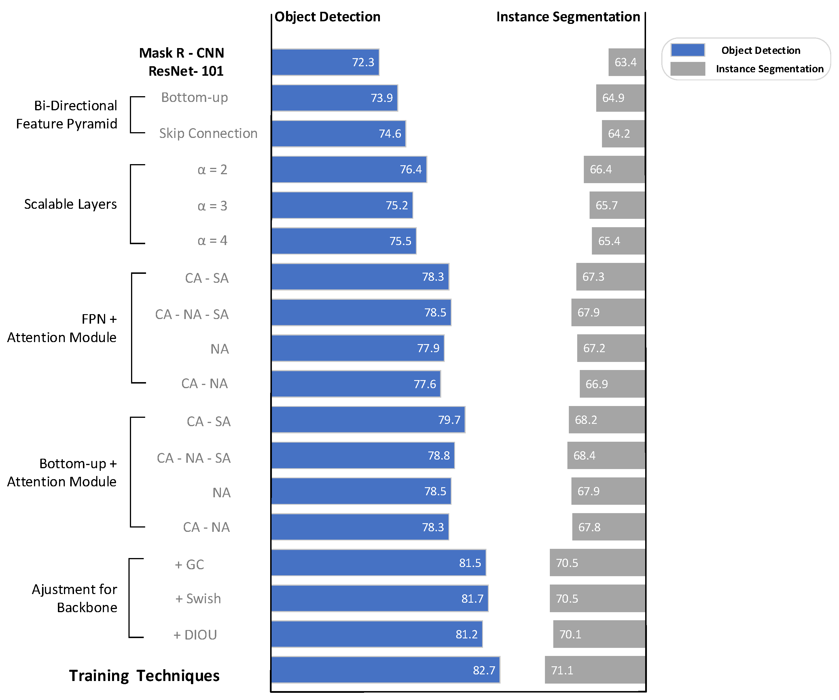
Figure 2.
Schematic diagram of bottom-up path feature fusion
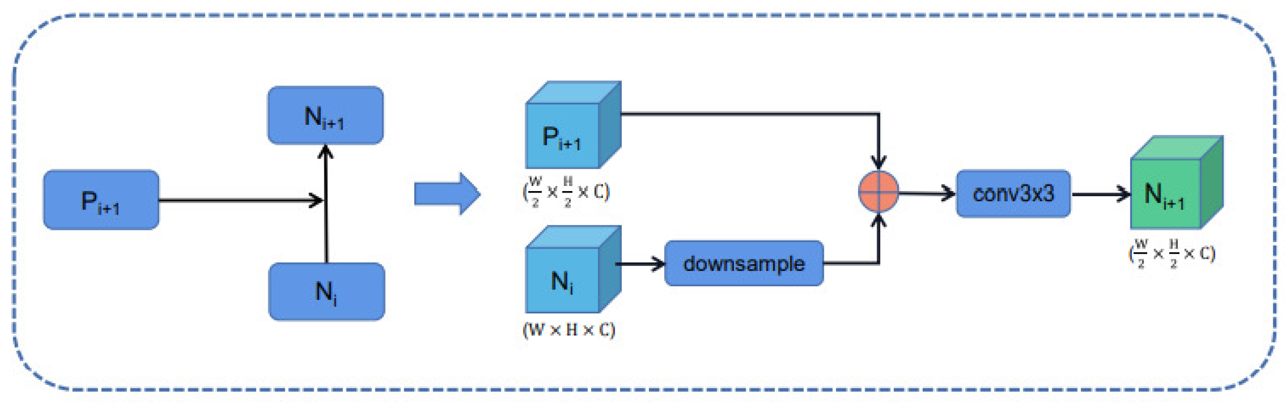
Figure 3.
Schematic diagram of the Bi-Directional Feature Pyramid.
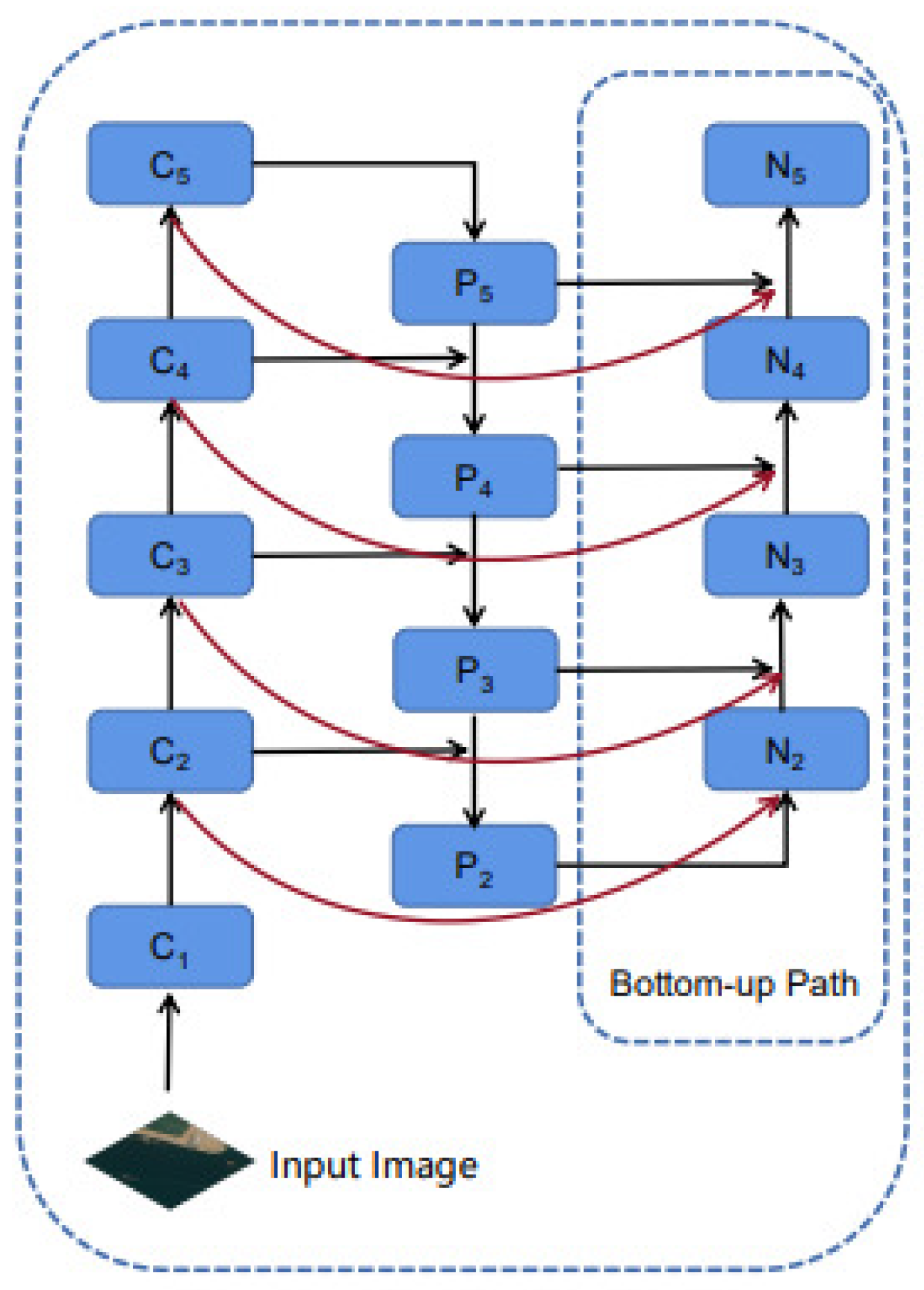
Figure 4.
Schematic diagram of feature fusion with Bottom-Up and Skip Connection.
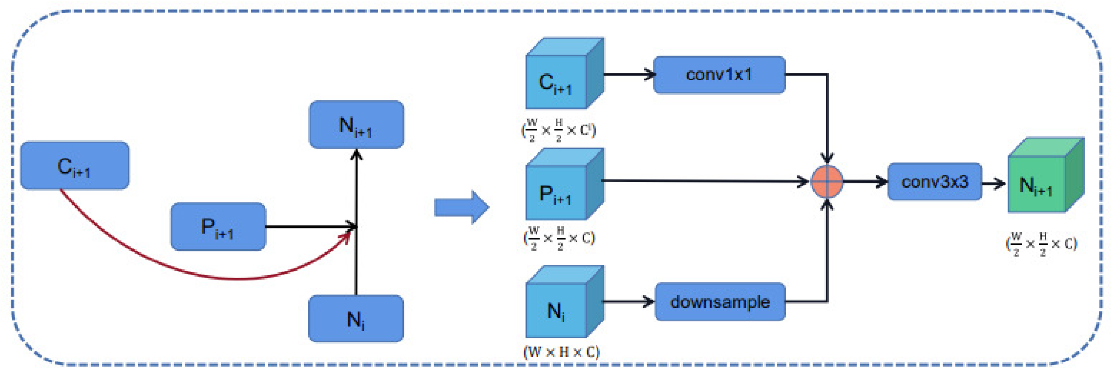
Figure 7.
Schematic diagram of Mixture-of-Experts (MoE) Attention Layer.
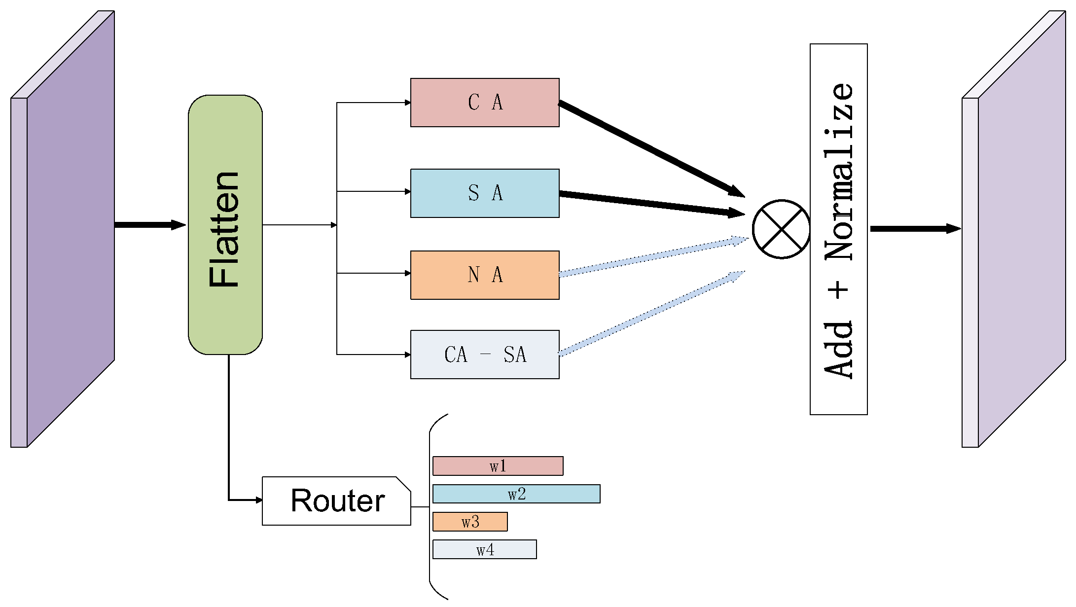
Figure 8.
Schematic diagram of self-attention node calculation.
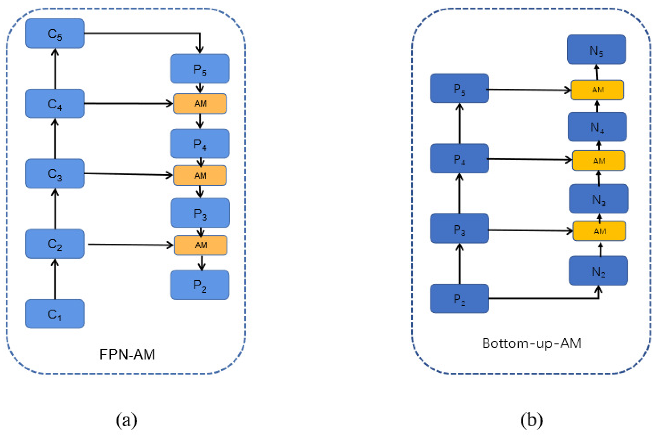
Figure 9.
(a) Schematic diagram of the channel-spatial attention module (CA_SA). (b) Schematic diagram of the parallel [channel-spatial] attention module.
Figure 9.
(a) Schematic diagram of the channel-spatial attention module (CA_SA). (b) Schematic diagram of the parallel [channel-spatial] attention module.
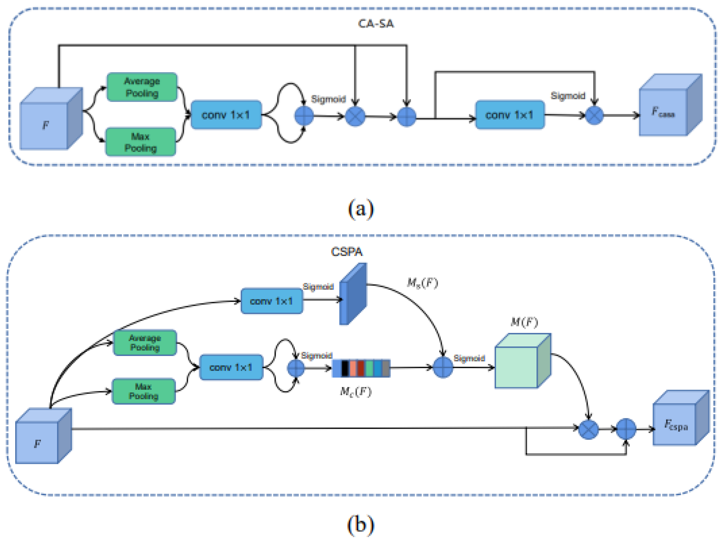
Figure 11.
Illustration of the building blocks of FPN-AM.
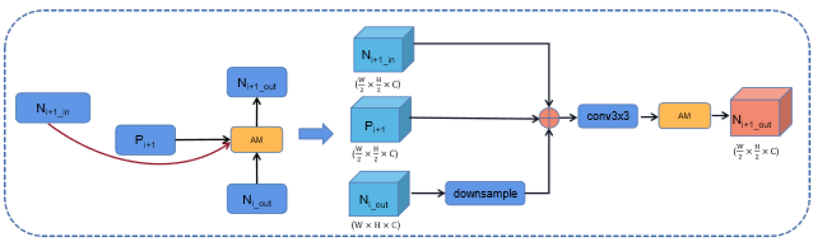
Figure 12.
Illustration of the building blocks of B-AM.
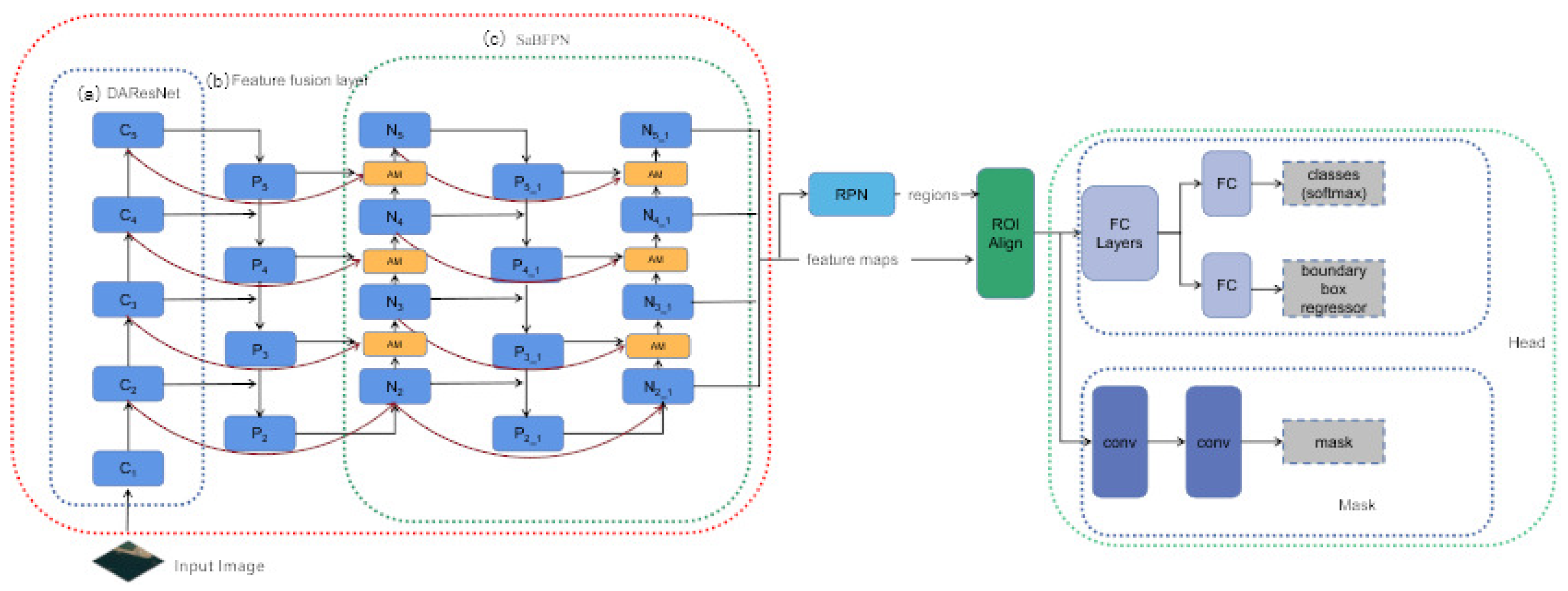
Figure 13.
Schematic diagram of improved Mask R-CNN with Attention Bi-Directional Feature Pyramid Structure.
Figure 13.
Schematic diagram of improved Mask R-CNN with Attention Bi-Directional Feature Pyramid Structure.
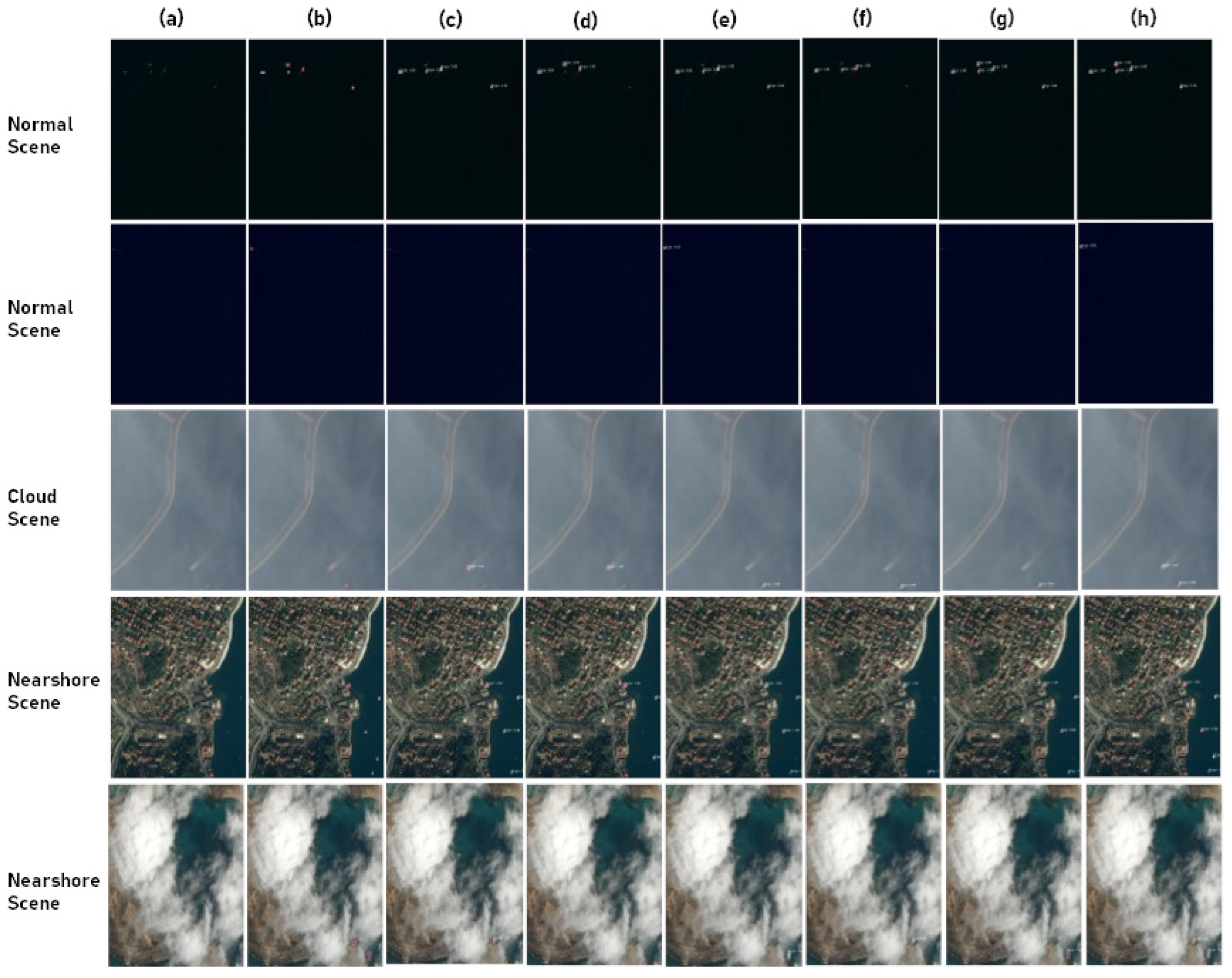
Figure 14.
Samples of ships detection and segmentation: (a) original images, (b) ground truths, (c) results from Mask R-CNN baseline model, (d) results from PANet, (e) results from Mask Scoring R-CNN model, (f) results from Mask R-CNN + NMS model, (g) results from Cascade Mask R-CNN model, (h) results from Ours. The detection and segmentation results under different noise scenes are shown respectively: Normal Scene, Cloud Scene, Nearshore Scene.
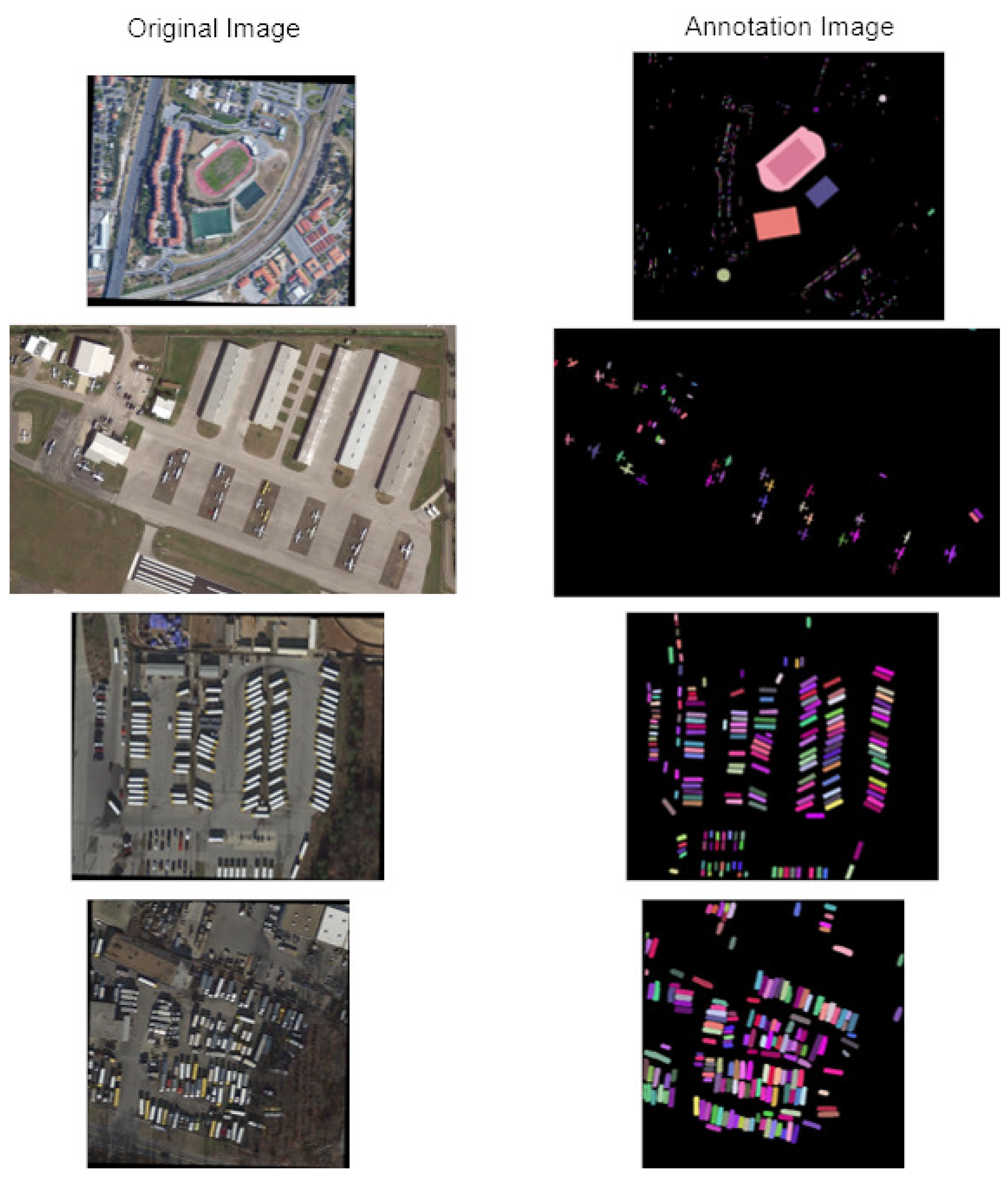
Figure 15.
Original Images, Annotation Images and Forecast Images of our method on Cityscape.
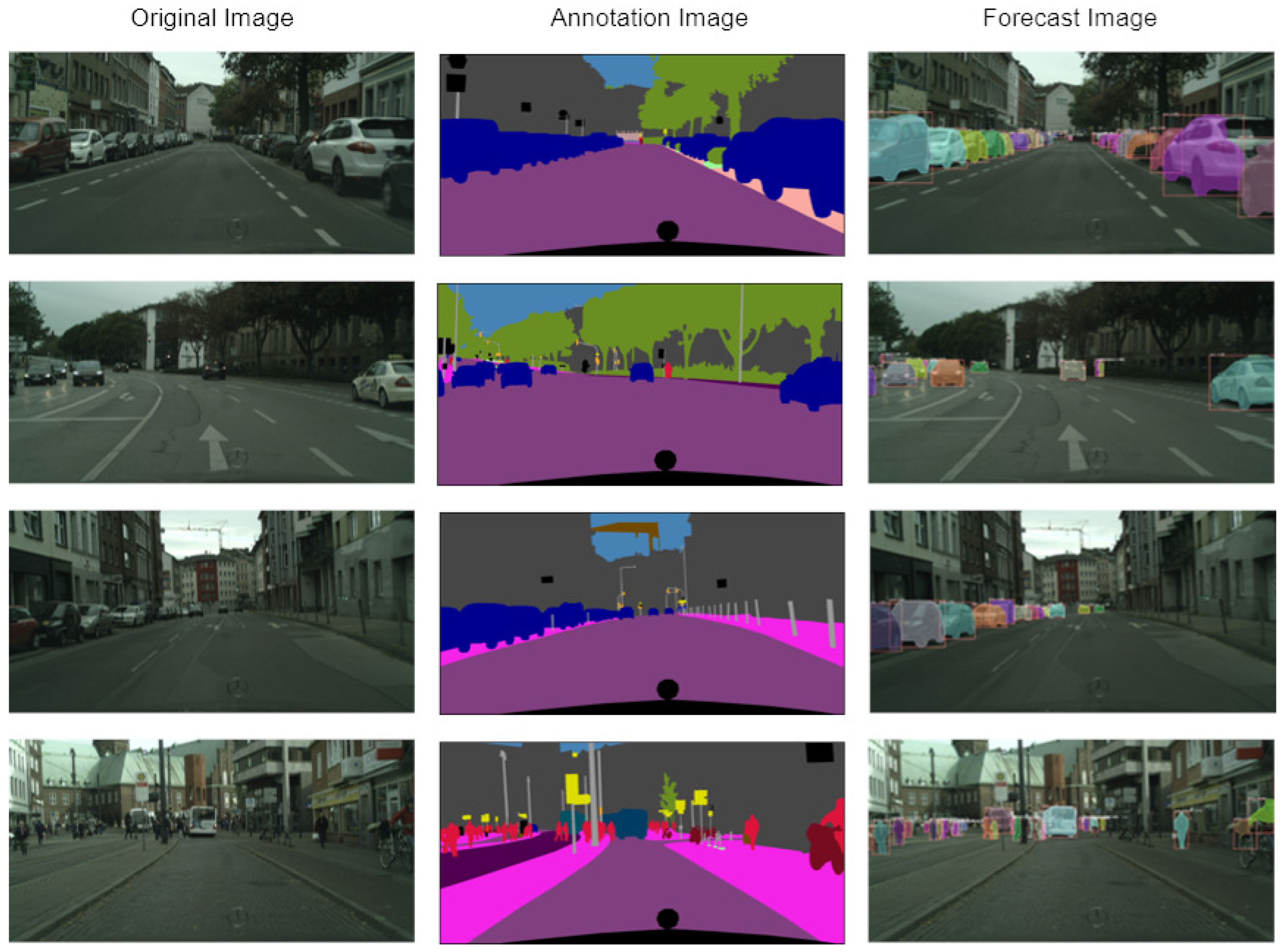
Figure 16.
Detection and segmentation results of different classes: (a) ship (b) Large-vehicle (c) ship (d) Small-vehicle.
Figure 16.
Detection and segmentation results of different classes: (a) ship (b) Large-vehicle (c) ship (d) Small-vehicle.
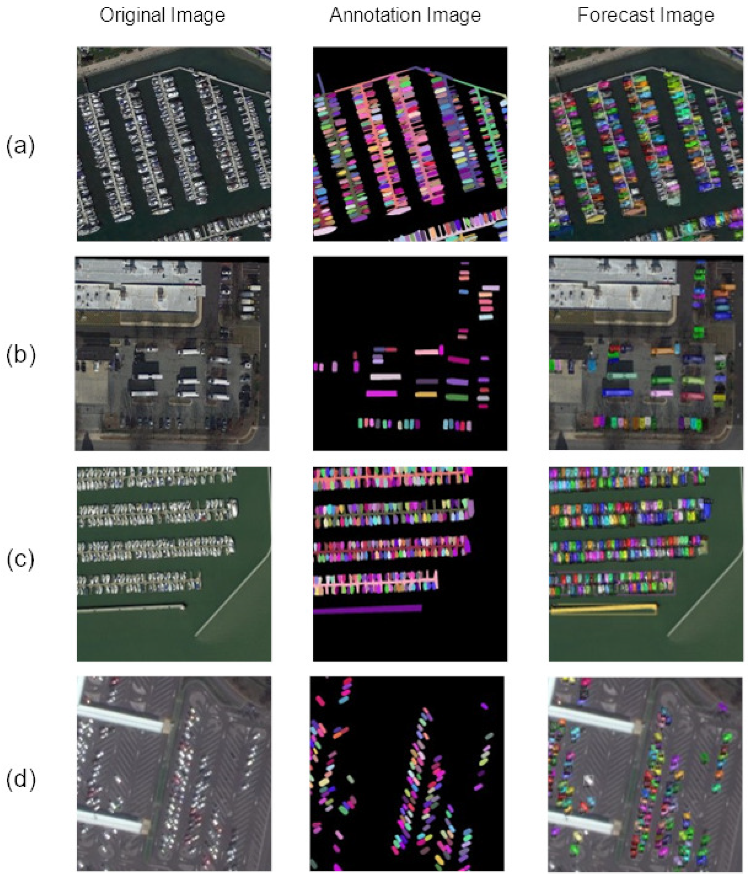
Table 1.
Detection/Segmentation Accuracy in the Ablation Study of Scalable Bi-directional Feature Pyramid Structure.
Table 1.
Detection/Segmentation Accuracy in the Ablation Study of Scalable Bi-directional Feature Pyramid Structure.
| Method | AP | |||||
| Mask R-CNN(baseline) | 71.3/61.4 | 94.6/90.8 | 81.7/71.8 | 63.2/50.8 | 86.6/79.1 | 87.2/84.1 |
| + B(Bottom up Path) | 73.9/63.9 | 94.9/91.3 | 82.2/72.7 | 64.8/52.9 | 87.4/81.2 | 86.0/83.8 |
| + B + SC(Skip Connection) | 74.6/65.7 | 95.0/91.6 | 84.5/73.2 | 64.4/54.7 | 87.9/81.9 | 88.8/85.9 |
| Number of feature fusion layer stacks | ||||||
| + B + SC + =2 | 76.4/66.4 | 95.6/92.3 | 85.6/74.3 | 68.2/55.3 | 89.8/83.7 | 89.4/87.0 |
| + B + SC + =3 | 75.2/65.7 | 95.2/92.6 | 84.7/74.8 | 67.8/54.8 | 88.3/83.2 | 90.8/86.3 |
| + B + SC + =4 | 75.5/65.4 | 95.3/92.0 | 84.9/73.7 | 67.2/54.6 | 89.2/82.9 | 90.3/86.7 |
Table 2.
Detection/Segmentation Accuracy in the Ablation Study of B-AM.
| Method | AP | |||||
| Mask R-CNN(baseline) | 71.3/ 62.4 | 94.6/ 90.8 | 81.7/71.8 | 63.2/ 50.8 | 86.6/ 79.1 | 87.2/ 84.1 |
| +B+SC+ | 76.4/ 66.4 | 95.6/ 92.3 | 85.6/74.3 | 68.2/ 55.3 | 89.8/ 83.7 | 89.4/ 87.0 |
| Bottom-up-AM(+B+SC+) | ||||||
| +CA | 77.3/ 67.1 | 96.1/ 93.8 | 86.9/76.9 | 72.2/ 57.3 | 90.5/84.9 | 90.8/ 87.2 |
| +SA | 77.7/ 66.9 | 95.7/ 94.3 | 87.2/ 77.2 | 72.7/ 56.9 | 90.3/ 84.2 | 90.5/ 87.5 |
| + NA | 78.5/ 67.9 | 96.8/ 94.6 | 87.7/ 77.9 | 72.3/ 57.0 | 90.9/ 85.1 | 91.5/ 86.9 |
| + CA-SA | 79.7/ 68.2 | 97.1/ 94.7 | 88.3/ 78.7 | 73.4/ 58.1 | 91.8/ 85.0 | 92.6/ 88.3 |
| + SA-CA | 79.0/ 68.0 | 96.6/ 94.5 | 87.9/ 78.1 | 73.2/ 58.4 | 91.1 / 85.2 | 91.7 91.7/ 88.7 |
| + CA-NA | 78.3/ 67.8 | 95.9/ 94.2 | 87.8/ 77.9 | 73.9/ 57.8 | 91.0 91.0/ 84.8 | 91.0 / 97.5 |
| + NA-CA | 77.8/ 67.4 | 96.3/ 93.9 | 87.3/ 77.8 | 73.5/ 57.4 | 90.6 /85.0 | 91.8/ /87.9 |
| + SA-NA | 78.7/ 67.7 | 96.0/ 94.2 | 88.0/ 78.3 | 72.5/ 58.0 | 91.5/ 85.0 | 92.3/ 88.6 |
| + NA-SA | 78.2/ 68.0 | 96.5/ 94.3 | 87.5/ 78.0 | 72.3/ 57.8 | 90.8/ 84.7 | 92.0/ 87.9 |
| +[CA-SA] | 77.2/66.8 | 95.3/ 94.0 | 86.7/76.9 | 71.2/ 56.3 | 90.6/ 83.9 | 90.2/87.0 |
Table 3.
Detection/ Segmentation Accuracy in the Ablation Study of Other Tricks, Including Introduction of Group Convolution, Introduction of Swish Activation Function, Replacement of Diou Loss Function, and Change of Training Strategy.
Table 3.
Detection/ Segmentation Accuracy in the Ablation Study of Other Tricks, Including Introduction of Group Convolution, Introduction of Swish Activation Function, Replacement of Diou Loss Function, and Change of Training Strategy.
| Method | AP | |||||
| Mask R-CNN(baseline) | 71.3/ 62.4 | 94.6/90.8 | 81.7/71.8 | 63.2/50.8 | 86.6/ 79.1 | 87.2/ 84.1 |
| +B+SC++B-AM(CA-SA) | 79.7/ 68.2 | 97.1/94.7 | 88.3/ 78.7 | 73.4/58.1 | 91.8/85.0 | 92.6/88.3 |
| +B +SC + = 2 + B - AM ( CA-SA ) | ||||||
| +GC(Group Convolution) | 81.5/70.5 | 97.1/94.9 | 89.7/ 79.8 | 74.8/ 60.2 | 93.0/86.2 | 92.6/ 88.6 |
| +Swich | 80.2/ 69.2 | 96.7/ 94.7 | 88.8/ 78.8 | 74.2/ 59.7 | 92.7/ 85.8 | 92.3/ 88.3 |
| +GC+Swich | 81.7/70.5 | 97.4/95.3 | 90.1/80.0 | 75.4/ 60.8 | 93.3/86.2 | 92.4/ 89.5 |
| +GC+Swich+DIoU | 81.2/70.1 | 97.0/ 94.9 | 89.7/ 79.0 | 73.9/ 59.3 | 92.9/85.9 | 92.1/ 89.1 |
| Training Techniques | 82.7/71.1 | 97.4/95.3 | 90.2/80.3 | 76.9/ 61.8 | 93.9/86.9 | 93.4/ 89.3 |
Disclaimer/Publisher’s Note: The statements, opinions and data contained in all publications are solely those of the individual author(s) and contributor(s) and not of MDPI and/or the editor(s). MDPI and/or the editor(s) disclaim responsibility for any injury to people or property resulting from any ideas, methods, instructions or products referred to in the content. |
© 2025 by the authors. Licensee MDPI, Basel, Switzerland. This article is an open access article distributed under the terms and conditions of the Creative Commons Attribution (CC BY) license (http://creativecommons.org/licenses/by/4.0/).
Copyright: This open access article is published under a Creative Commons CC BY 4.0 license, which permit the free download, distribution, and reuse, provided that the author and preprint are cited in any reuse.


