
Submitted:
06 March 2025
Posted:
07 March 2025
You are already at the latest version
Abstract
Edge-computing applications require of ultra-low power architectures for both the feature extraction and the classifier stages. In this manuscript a complete architecture for these applications is proposed making use of an analog-based feature extraction stage composed of a bank of band-pass filters, and a 4-bit weight, 8-bit activation function learned step size (LSQ) quantized gated recurrent unit (GRU)-based classifier stage for keyword spotting (KWS) systems. The proposed KWS architecture achieves 91.35% of accuracy for 12 classes including 10 keywords from the Google Speech Command Dataset v2 (GSCDv2), with less than 1% accuracy loss compared to full precision classification, with an estimated memory footprint of 34.8 kB and 62 400 multiply–accumulate (MAC) operations per inference in real-time mode.
Keywords:
keyword spotting (KWS)
; quantization-aware training (QAT)
; analog feature extraction
; recurrent neural network (RNN)
; edge computing
1. Introduction
With the advancement of portable devices and artificial intelligence (AI) techniques, the demand for energy efficient processing sensor data on the edge has been rapidly increased. Edge computing offers significant benefits over remote cloud-based processing that includes reduced data transmission bandwidth, lower latency, and enhanced sensitive data privacy at the expense of extremely restricted power requirements [1]. Energy efficiency is critical for edge computing due to the constraints of limited battery capacity or reliance on energy harvesting circuits. This usually leads to simpler classification and regression circuit architectures with weaker pattern recognition capabilities than complex algorithms executed in CPU/GPUs. Ultra-low power structures are then required to enlarge the number of processing elements and achieving sufficiently high accuracy and resolution performance [2].
A foundational edge-AI application is Keyword Spotting (KWS), widely utilized in human-machine interaction scenarios such as virtual reality or automatic speech recognition (ASR). Acting as a power-gating mechanism, KWS triggers downstream function blocks only when a command word is detected, enabling voice-activated devices. In the same context, Voice Activity Detection (VAD) systems are simplified versions of KWS architectures designed only to distinguish between whether a sound corresponds to human voice or not [3,4]. The always-on and smart nature of either VAD or KWS systems requires a trade-off between classification simplicity and performance, and power efficiency.
Figure 1 depicts the conventional architecture of a KWS system. It is composed of an analog front-end (AFE) that makes filtering, amplification and digitization operations, and a digital back-end that performs intensive machine learning computation to extract data features and classify them [5,6]. While this approach often leads to excellent classification performance, it may not be suitable to the requirements of edge-computing due to the strong power-hungry nature of the solution. In an attempt to reduce such power consumption, many works have focused on carrying typically digital-based operations to the analog domain, where they might occupy more silicon area, but show much higher energy efficiency [7,8]. Splitting up the smart computing steps into the feature extraction and the classification steps, some works where analog-based feature extraction stages are proposed are [9,10], and also those where both stages work in the analog domain are [3,11]. The analog nature of the solutions enable architectures with a power consumption of less than 100 W. Finally a recent trend is towards neuromorphic based systems for ultra-low power devices both in the analog [12] and in the digital domain [13].
The current manuscript is framed within the context described above, looking for energy efficient solutions for edge-located KWS environments. To address the previous challenges, a highly energy efficient gated recurrent unit (GRU)-based KWS with analog-based feature extraction is proposed. Excellent state-of-the-art classification accuracy is achieved with reduced model complexity and hardware-aware optimizations. This work introduces several key innovations that distinguish our approach from prior state-of-the-art. The main contributions are listed below:
- 1.
- Outstanding trade-off between classification accuracy and complexity. The proposed KWS system employs the same analog feature extraction configuration as in [9], and achieves a higher accuracy of 92.33% with the full precision model and 91.35% with the quantized model, compared to 91.00% of [9]. Pattern classification is made by a simple GRU-based structure, utilizing only 80 neurons per layer, compared to 128 neurons needed in [9].
- 2.
- Use of Learn Step Size (LSQ) and Look-Up Table (LUT)-Aware Quantization for high efficient computation, unlike previous works that use post-training quantization or fixed-point quantization. This approach enables adaptive quantization during training, reducing power and memory consumption while maintaining high recognition accuracy. The proposed model operates with 4-bit weights and 8-bit activation functions, significantly reducing computational complexity compared to prior works that rely on 8-bit weights and 12- or higher bit activation functions [11,14].
The document has the structure outlined below. Section 2 shows the foundations of the KWS system, focusing on the analog-based feature extraction stage and the digital GRU-based classifier. Section 3 describes the LSQ methodology used to train the classifier stage. Section 4 presents the dataset for training and inference, and discuss the obtained results. Finally, Section 5 concludes the manuscript.
2. Description of the Proposed KWS Architecture
A schematic diagram of the KWS is shown in Figure 2. The system consists of a microphone as the sensing stage, a 16-channel log-spaced analog filter bank, an analog frame and energy extractor, and a sampling block, followed by a GRU-based digital classifier. The classifier comprises two GRU-based layers, each with 80 units, concluding with a fully connected (FC) classification layer with 12 output neurons, corresponding to the 12 classes.
2.1. Analog Filter Bank Feature Extractor
A conventional approach to extract the audio features in the analog domain is illustrated in Figure 3. The process begins with a set of analog band-pass filters, each tuned to a different center frequency, which are connected to the raw audio input signal. Next, wave rectifiers convert the filtered signals into their envelope representations. Finally, the energy within each frame is estimated by integrating the rectified signal over the frame’s time step.
The transfer function of the band-pass filters can be expressed as follows:
where represents the center frequency of the filter, and Q is the quality factor. The same filter bank configuration as in [9] is used, implementing 16 log-spaced band-pass filters with the center frequencies ranging from 125 Hz to 5 kHz and a quality factor of 4.5. Figure 4 shows the frequency response of the 16 band-pass filters. To ensure consistent amplitude scaling, a gain control mechanism is applied, normalizing each filter to unit gain at its center frequency.
To mimic the analog-domain rectification and integration over a frame duration in the feature extraction process applied to the filtered signal, the energy of each frame in our software model is computed using the following equation:
where represents the energy of the n-th frame, which consists of N sampled points withing this frame.
As an example, Figure 5a illustrates the time-domain waveform and the corresponding filter bank representation of the keyword "yes", using a 10 ms frame window with a 10 ms frame shift. The top plot shows the raw waveform, where the temporal structure of the word can be observed. The phonemes in the keyword "yes" are annotated, highlighting the transition from the initial "Ye" sound to the final "s" sound. The bottom heatmap represents the filtered energy distribution over time across the 16 log-spaced frequency channels. The x-axis corresponds to the time frames and the y-axis represents the filter bank channels sorted from the lowest to the highest frequency. It can be appreciated that the "Ye" sound exhibits stronger low-frequency energy, and the "s" sound higher frequency components. Figure 5b provides a more detailed visualization of the band-pass filtering process, where the original waveform (blue) and the filtered waveforms (orange) are shown for multiple band-pass filters with different center frequencies. As expected, low-frequency filters (e.g., 125 Hz, 204 Hz, 334 Hz) capture the low-frequency components of the speech signal, while higher-frequency filters (e.g., 1462 Hz, 2390 Hz, 3909 Hz) emphasize the higher frequency phoneme information. This analysis confirms that our log-spaced analog filter bank effectively decomposes the speech signal into frequency bands, allowing the downstream classifier to capture the required temporal and spectral patterns for keyword spotting.
2.2. GRU-Based Classifier
In [15], various neural network architectures were trained and compared for KWS targeted on hardware resource-constrained microcontrollers. It was demonstrated that Recursive Neural Network (RNN) models, including the Long-Short Term Memory (LSTM) or GRU models, outperformed their counterparts like Convolutional Neural Networks (CNNs) or standard feed-forward models in classification accuracy, memory footprint, and number of operations per inference. Although convolutional RNN (CRNN) or depth-wise separable CNN (DS-CNN) showed even better performance than RNNs, they require access to the full receptive field of the input such as a large amount of the input audio frames, which will increase the latency due to the input window buffering. In contrast, RNN models can process one input frame at a time, maintaining an internal state across frames. This allows RNNs to process audio data as it streams, making them inherently suited for sensor applications where the sensor frequency is limited [16].
The two most popular RNN variants are LSTM and GRU. They capture the temporal dependencies of the speech signals and model the time-varying nature of them with their internal gate mechanism, and mitigate the vanishing gradient problem that emerges in the vanilla RNN model when the sequence becomes longer. GRU models are simpler than LSTM ones because they have one fewer gate reducing the computing complexity, and thus are preferred in the integrated circuit community [9,11]. Additionally, there are other edge devices optimized RNN variants applied in KWS application, such as skip RNN [14,17] and -GRU [13,18]. These variants are more power efficient combined with specific AFEs and digital feature extraction circuits. Given the current approach of this work for edge-computing environments a standard GRU architecture is adopted. Yet, the more advanced architecture like Fast-RNN [19] or Mamba [20] are also potential suitable candidates and will be considered in future works.
Increasing the number of units per layer and the number of layers in a GRU generally enhances the capability to capture complex patterns from input data and process them within multiple levels of abstraction. This improvement is particularly beneficial for KWS tasks involving classifying and detecting a large amount of words, phonetically similar keywords, or dealing with noisy conditions. Nevertheless, it comes at the cost of increased complexity and computational demand, posing significant challenges for their deployment on edge devices.
Figure 6 illustrates how the accuracy performance of GRU-based classifiers depends on the number of units per layer (Figure 6a) and on the number of hidden layers (Figure 6b), demonstrating that, while not incurring overfitting, the performance improves with deeper GRU models. For this particular case, overfitting is observed with too complex models, as seen in Figure 6a for a number of units per layer higher than 110. Note that all other hyperparameters remain constant during training and may not be fully optimized, as will be discussed in Section 4.2. As we aim to train a model with an overall accuracy above 90% while keeping the size as small as possible, 80 units are selected per each hidden layer and a depth of 2 hidden layers are selected in this work. A fully-connected layer is finally added to perform the classification task.
3. Learned Step Size Quantized GRU Classifier
3.1. Background
In [21] a comprehensive survey on the efficient compression and execution of deep neural networks from both algorithms and hardware perspectives is provided. According to the authors, quantizing RNNs is more challenging than quantizing CNNs due to the recurrent nature and internal state dependence of RNNs. Quantization errors can propagate and accumulate across multiple time steps and significantly impact performance. Complex RNN structures, such as GRU and LSTM units, rely on gating mechanisms and sophisticated non-linear operations like sigmoid and tanh functions, which are particularly sensitive to limited precision.
An integer-only quantization method was proposed for CNNs in [22]. This method was later adapted to RNNs, as shown in [16,23,24], but was limited to the post-training quantization stage (PTQ). In their approach, a real number r is quantized using the following equation:
where is the quantized value of the real number r, and denote the quantization range respectively, and S and Z are the scale and the zero points, defined by:
where is weight or activation tensor with any shape and is the total bit-width.
Another quantization method applied to RNNs is fixed-point quantization [11,13], represented in Qi.f format, where i and f denote the number of bits before and after the decimal point, respectively. A real number r can be then quantized using the following equations:
where ≪ and ≫ represent bit shifting operations, and and are the quantized and de-quantized values of a real number r, respectively. The challenge of fixed-point quantization lies in defining the word and the integer lengths, i.e., selecting the position of the binary point for a given bit-width. This requires an in-depth analysis of the dynamic range of the weights and activation functions in an already trained full-precision model. Based on this analysis, the appropriate word length and integer length are chosen to quantize the model effectively.
Instead of statically setting the scaling factor S and the zero point Z as shown in Equations (4) and (), the LSQ quantization method [25,26] learns these parameters during training. This approach optimizes the model weights, scaling factors, and zero points simultaneously to reduce quantization error, leading to improved performance compared to static quantization. While most existing studies focus on applying LSQ to CNNs, research works on LSQ for RNNs is limited. To the best of our knowledge, this work is the first to apply LSQ on a GRU-based classifier for KWS applications. The proposed method will be described in detail in the following subsection.
3.2. Methodology
The terminology of Pytorch [27] is followed for the GRU implementation:
where is the input data at time t, is the hidden state at time t, is the hidden state at time or the initial hidden state at time 0, and are the reset, update, and new gate, respectively, denotes the sigmoid function, and ⊙ represents the Hadamard (element-wise) product. The learnable weights and biases are divided into input-to-hidden and hidden-to-hidden parts.
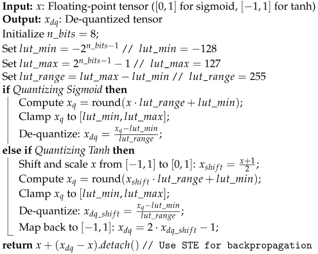
Figure 7 shows the data flow of a GRU unit with fake quantization nodes (FQNs) inserted for both activation functions and weights in the quantization-aware training (QAT), bias terms are omitted for the sake of simplicity. FQNs with LUT-based approximation are placed in the reset, update, and new gate outputs. Using a shared LUT across multiple GRU layers for both sigmoid and hyperbolic tangent (tanh) activations in future hardware deployment is expected. Since tanh function can be derived from the sigmoid value using the relation , this approach improves hardware efficiency. The behavior of these nodes is described in Algorithm 1, with an 8-bit LUT covering the range [-128, 127]. During forward propagation in QAT, the de-quantized sigmoid or tanh tensors are passed, while in backpropagation, gradients are computed using the Straight-Through Estimator (STE) [28].
FQNs with learnable parameters are inserted for weight tensors, the hidden state () output, the feature input tensor in the first GRU layer, and the final fully connected classification layer output, as depicted in Figure 8. Their behavior is described in Algorithm 2.
| Algorithm 1: Quantization for Sigmoid and Tanh with LUT Approximation |
 |
| Algorithm 2: Learned Step Size Quantization (LSQ) with Gradient Scaling |
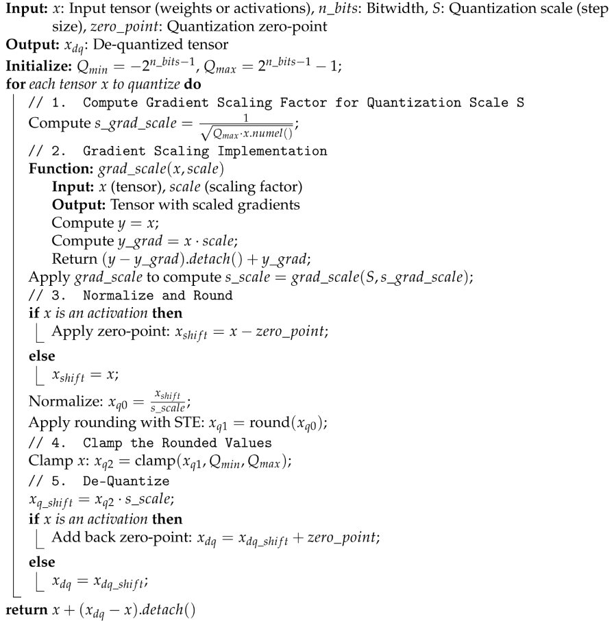 |
During training, in forward pass, these learnable FQNs take the floating point input tensor and return the de-quantized tensors using the following equations
To balance computational efficiency and model performance, the quantization zero point Z is omitted for weight tensors () but retained for activations. This choice is based on an analysis of the pre-trained full-precision model, which reveals that weight distributions are predominantly symmetric, whereas activations exhibit greater asymmetry.
According to [25], the scaled gradient for the learnable quantization step size S is calculated as , with representing the total number of elements in the tensor . This formula ensures that, for different step sizes across various tensors and layers, the ratio of update magnitude to parameter magnitude remains consistent. This consistency is crucial for stable training and good convergence. The function in Algorithm 2 returns the step size to quantize the tensor S during forward pass, while providing the properly scaled gradient during backward pass to update S itself. In contrast, the quantization zero point Z in our work is updated directly using the learning rate. However, this can be further improved by adopting an optimized updating mechanism similar to S, as proposed in [26].
4. Training, Performance Results and Comparison
4.1. Data Preparation
We use Google Speech Command Dataset v2 (GSCSv2) to train and evaluate the proposed neural network [29]. The dataset includes 35 words and consists of 105 829 one-second (or less) audio clips recorded by 2618 speakers. The downloaded dataset 1 comes with already partitioned training, validation, and test sets 2, such that the keywords spoken by a given speaker always remain in the same set. Besides, the dataset includes several minute-long background noise files. The KWS model is trained for a 12-class classification task. Ten words are selected as the desired keywords and the rest 25 words are grouped into the "Unknown" class. The additional "Silence" class includes multiple 1-second clips randomly sampled from the background noise files. The training set consists of 38 863 samples, including those from the 10 target keyword classes, 4044 "Silence" samples, and 4050 "Unknown" samples. The "Silence" samples are randomly generated from background noise tracks, with volume levels uniformly distributed between -30 dB and 0 dB. The "Unknown" samples are selected from non-target words, ensuring equal representation of each word. The validation set, based on the official partition, contains 4503 samples, with an additional 400 samples each for the "Silence" and "Unknown" classes. The standard test set is used without modification, containing 4890 samples, with approximately 400 samples per class across the 12 classification categories. This results in a training, validation, and test set ratio of roughly 8:1:1, with balanced occurrence of each class within each set.
4.2. Training
First, a full-precision model is built using the Pytorch 2.4 framework and trained with Optuna [30] for hyperparameter optimization. The Tree-structured Parzen Estimator (TPE) sampler and median pruner are employed in Optuna, with overall validation accuracy as the optimization metric. The model is trained with the AdamW optimizer [31], cross-entropy loss function, and the ReduceLRonPlateau learning rate scheduler.
The hyperparameters search space includes:
- Number of epochs: 20 to 150;
- Batch size: 16 to 256;
- Learning rate: 1e-5 to 0.1;
- Weight decay: 1e-6 to 0.01;
- GRU dropout: 0.0 to 0.5;
- Learning rate scheduler decay factor: 0.1 to 0.9.
100 Optuna search trials with 30 trials patience are set for early stopping. The final trained full-precision model achieves an overall accuracy of 92.33%.
To mitigate performance degradation during model quantization, a two-step quantization strategy is adopted, where activation functions and weights are quantized separately. First, the activation functions are quantized while keeping weights in full precision, as activation quantization has a more immediate impact on inference accuracy than weight quantization. This activation-only quantized model is initialized using the parameters of the full-precision model. Next, this activation-quantized model is used to initialize the fully quantized model, where both activations and weights are quantized. This progressive quantization approach enhances training stability, allowing the quantized model to converge faster and reducing the required training epochs.
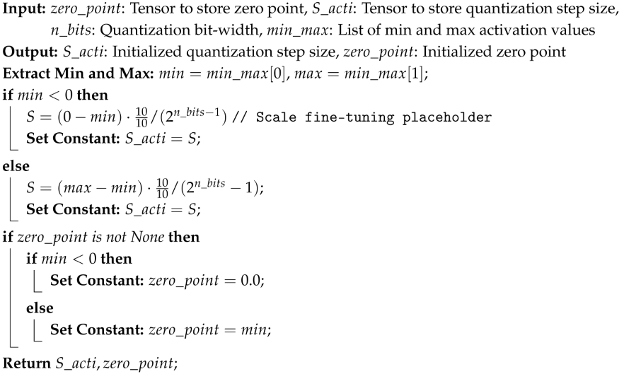
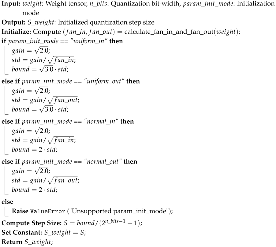
After initializing the quantized model with pretrained weights and biases, a forward pass over the entire training dataset is performed to estimate the activation range using a moving average window. The activation quantization parameters are initialized using Algorithm 3, following a static determination method, as defined in Equations 4 and . The weight quantization step size S is initialized using the Kaiming He method [32], ensuring that weight values are well distributed within their bit-width constraints, as described in Algorithm 4. For weight tensor quantization, the zero point is set to 0 to maintain symmetry, based on observations of trained full precision model weight distributions.
For both the activation-quantized and fully quantized models, the Optuna search space is minimized by tuning only the learning rate and weight decay, while keeping other hyperparameters constant. This decision is based on some observations from Optuna hyperparameter tuning during full-precision training, where these parameters have had the most significant impact on performance.
Through experiments exploring various weight and activation bit-widths in QAT, the final quantized model adopts 4-bit weights and 8-bit activations for GRU layers, while the final classification layer utilizes 8-bit weights and 8-bit activations. This choice aligns with findings in [25], which suggest that maintaining higher precision in the final layer enhances overall model performance. The selected quantization scheme effectively reduces model size while preserving accuracy.
| Algorithm 3: Initialization of Activation Quantization Step Size and Zero Point |
 |
| Algorithm 4: Initialization of Weight Quantization Step Size |
 |
4.3. Results and Discussion
The final quantized KWS model achieves an overall accuracy of 91.35% on the 12-class GSCDv2 dataset (10 keywords + "Unknown" and "Silence"), with an accuracy loss of less than 1% compared to the 92.33% achieved by the full-precision model. This result demonstrates that the quantization strategy, based on LSQ and fine-tuning techniques, effectively preserves model performance while significantly reducing computational complexity. Figure 9 shows the true positive rate (TPR) confusion matrix for the 12-class classification task. The quantized model performs well across most classes, with TPRs exceeding 90% for most keywords, highlighting the effectiveness of our KWS system. However, despite achieving 100% TPR for the "Silence" class and performing strongly on words such as "yes" and "right", which have longer durations and distinct spectral peaks, the model struggles with short-duration words or those with diffuse energy distributions, such as "no" and "up". The most challenging class is "Unknown", which includes 25 non-target words, introducing high variability. This variability poses a significant challenge for the simple both analog filter-bank feature extractor (FEx) and GRU classifier.
The authors would like to advance that the model performance could be even further improved at the expense of increased power and area consumption as is the case of other works such as [15,33,34]. Potential enhancements include a more advanced feature extraction stage, integrating logarithmic energy scaling or energy derivatives to better capture speech dynamics, and a larger GRU model, capable of learning more complex temporal relationships in the extracted features.
The memory size of the proposed model is estimated by multiplying the number of weights and biases by their respective widths. With a parameter size of 63 372 (excluding quantization parameters), the estimated memory requirement is only 34.8 kB, considering 4-bit weights and 32-bit biases. The number of multiply-and-accumulate (MAC) operations per inference is given by , where B and T denote the batch size and number of time steps in the input sequence, respectively. In real-time mode, the model processes one frame per time step, requiring 62 400 MAC operations inference. In [15] three sets of computational constraints were defined for small, medium, and large microcontroller systems running KWS applications. Based on their analysis, the KWS system of this work easily meets the requirements for small hardware systems, offering a tiny memory footprint and a light computation burden per inference, making it well-suited for low-power edge deployment.
Table 1 compares this work with other state-of-the-art KWS systems implemented on silicon. All these systems employ RNN variants as classifiers and use the GSCD dataset (v1 and v2 versions). Compared to prior works, the proposed KWS system achieves the highest accuracy on the 12-class, 10-keyword dataset, making use of an analog feature extraction stage to save power and a lightweight classifier with only 80 units per recurrent layer. The introduced Learn Step Size (LSQ) and LUT-aware quantization method enables to propose the lowest bit-width computation for weights and activation functions. The larger required memory in comparison to other works is due to the higher number of units.
5. Conclusions
In this paper, we introduce a potentially power-efficient KWS system composed of an analog filter-bank-based feature extraction stage and a GRU-based classifier. The applied Learn Step Size (LSQ) and LUT-aware quantization method ensures low bit-width computation, reducing weights to 4 bits and activation functions to 8 bits in the classifier. The proposed system achieves an overall accuracy of 91.35% on the GSCDv2 dataset for 12 classes with 10 keywords, which means a higher accuracy in comparison to other quantized KWS systems of the literature. Based on our estimation, the model requires only 34.8 kB of weight memory and 62 400 MAC operations per inference in real-time operation mode. The analog nature of the feature extraction, high classification accuracy, tiny memory footprint, and lightweight computational requirements make the proposed KWS system extremely suitable for deployment on low power edge devices.
Author Contributions
Conceptualization, Y.S. and E.G.; methodology, Y.S., B.W., and E.G.; software, Y.S. and B.W.; validation, Y.S.; formal analysis, Y.S. and E.G.; investigation, Y.S. and B.W.; resources, E.G.; data curation, Y.S.; writing—original draft preparation, Y.S. and E.G.; writing—review and editing, Y.S. and E.G.; visualization, Y.S.; supervision, E.G. and D.S.; project administration, E.G.; funding acquisition, E.G. All authors have read and agreed to the published version of the manuscript.
Funding
This research was funded by program H2020-MSCA-ITN-2020, grant No. 956601, and by Agencia Estatal de Investigacion (AEI), Spain, under Grant PID2020-118804RB-I00VCO.
Institutional Review Board Statement
Not applicable.
Informed Consent Statement
Not applicable.
Data Availability Statement
Data are available upon request.
Conflicts of Interest
The authors declare no conflicts of interest.
Abbreviations
The following abbreviations are used in this manuscript:
| LSQ | Learned step size |
| GRU | Gated recurrent unit |
| KWS | Keyword spotting |
| GSCDv2 | Google speech command dataset v2 |
| MAC | Multiply-accumulate |
| AI | Artificial intelligence |
| ASR | Automatic speech recognition |
| VAD | Voice activity detection |
| AFE | Analog front-end |
| LUT | Loop-up table |
| FC | fully connected |
| RNN | Recurrent neural network |
| LSTM | Long-short term memory |
| CNN | Convolutional neural network |
| CRNN | Convolutional recurrent neural network |
| DS-CNN | Depth-wise separable convolutional neural network |
| PTQ | Post-training quantization |
| QAT | Quantization-aware training |
| FQN | Fake quantization node |
| STE | Straight-through estimator |
| TPE | Tree-structured parzen estimator |
| TPR | True positive rate |
| FEx | Feature extractor |
References
- Shi, W.; Cao, J.; Zhang, Q.; Li, Y.; Xu, L. Edge Computing: Vision and Challenges. IEEE Internet of Things Journal 2016, 3, 637–646. [Google Scholar] [CrossRef]
- Yu, C.H.; Kim, H.E.; Shin, S.; Bong, K.; Kim, H.; Boo, Y.; Bae, J.; Kwon, M.; Charfi, K.; Kim, J.; et al. 2.4 ATOMUS: A 5nm 32TFLOPS/128TOPS ML System-on-Chip for Latency Critical Applications. In Proceedings of the 2024 IEEE International Solid-State Circuits Conference (ISSCC), 2024, Vol. 67, pp. 42–44. [CrossRef]
- Yang, M.; Yeh, C.H.; Zhou, Y.; Cerqueira, J.P.; Lazar, A.A.; Seok, M. Design of an Always-On Deep Neural Network-Based 1- μ W Voice Activity Detector Aided With a Customized Software Model for Analog Feature Extraction. IEEE Journal of Solid-State Circuits 2019, 54, 1764–1777. [Google Scholar] [CrossRef]
- Shen, Y.; Straeussnigg, D.; Gutierrez, E. Towards Ultra-Low Power Consumption VAD Architectures with Mixed Signal Circuits. In Proceedings of the 2023 IEEE International Symposium on Circuits and Systems (ISCAS); 2023; pp. 1–5. [Google Scholar] [CrossRef]
- Shan, W.; Yang, M.; Wang, T.; Lu, Y.; Cai, H.; Zhu, L.; Xu, J.; Wu, C.; Shi, L.; Yang, J. A 510-nW Wake-Up Keyword-Spotting Chip Using Serial-FFT-Based MFCC and Binarized Depthwise Separable CNN in 28-nm CMOS. IEEE Journal of Solid-State Circuits 2021, 56, 151–164. [Google Scholar] [CrossRef]
- Kawada, A.; Kobayashi, K.; Shin, J.; Sumikawa, R.; Hamada, M.; Kosuge, A. A 250.3μW Versatile Sound Feature Extractor Using 1024-point FFT 64-ch LogMel Filter in 40nm CMOS. In Proceedings of the 2024 IEEE Asia Pacific Conference on Circuits and Systems (APCCAS), Nov 2024, pp. 183–187. [CrossRef]
- Gutierrez, E.; Perez, C.; Hernandez, F.; Hernandez, L. Time-Encoding-Based Ultra-Low Power Features Extraction Circuit for Speech Recognition Tasks. Electronics 2020, 9. [Google Scholar] [CrossRef]
- Shen, Y.; Perez, C.; Straeussnigg, D.; Gutierrez, E. Time-Encoded Mostly Digital Feature Extraction for Voice Activity Detection Tasks. In Proceedings of the 2024 IEEE International Symposium on Circuits and Systems (ISCAS); 2024; pp. 1–5. [Google Scholar] [CrossRef]
- Mostafa, A.; Hardy, E.; Badets, F. 17.8 0.4V 988nW Time-Domain Audio Feature Extraction for Keyword Spotting Using Injection-Locked Oscillators. In Proceedings of the 2024 IEEE International Solid-State Circuits Conference (ISSCC), 2024, Vol. 67, pp. 328–330. [CrossRef]
- Croce, M.; Friend, B.; Nesta, F.; Crespi, L.; Malcovati, P.; Baschirotto, A. A 760-nW, 180-nm CMOS Fully Analog Voice Activity Detection System for Domestic Environment. IEEE Journal of Solid-State Circuits 2021, 56, 778–787. [Google Scholar] [CrossRef]
- Kim, K.; Gao, C.; Graça, R.; Kiselev, I.; Yoo, H.J.; Delbruck, T.; Liu, S.C. A 23-μW Keyword Spotting IC With Ring-Oscillator-Based Time-Domain Feature Extraction. IEEE Journal of Solid-State Circuits 2022, 57, 3298–3311. [Google Scholar] [CrossRef]
- Narayanan, S.; Cartiglia, M.; Rubino, A.; Lego, C.; Frenkel, C.; Indiveri, G. SPAIC: A sub-μW/Channel, 16-Channel General-Purpose Event-Based Analog Front-End with Dual-Mode Encoders. In Proceedings of the 2023 IEEE Biomedical Circuits and Systems Conference (BioCAS), Oct 2023; pp. 1–5. [Google Scholar] [CrossRef]
- Chen, Q.; Kim, K.; Gao, C.; Zhou, S.; Jang, T.; Delbruck, T.; Liu, S.C. DeltaKWS: A 65nm 36nJ/Decision Bio-inspired Temporal-Sparsity-Aware Digital Keyword Spotting IC with 0.6V Near-Threshold SRAM. IEEE Transactions on Circuits and Systems for Artificial Intelligence 2024, pp. 1–9. [CrossRef]
- Yang, H.; Seol, J.H.; Rothe, R.; Fan, Z.; Zhang, Q.; Kim, H.S.; Blaauw, D.; Sylvester, D. A 1.5-μW Fully-Integrated Keyword Spotting SoC in 28-nm CMOS With Skip-RNN and Fast-Settling Analog Frontend for Adaptive Frame Skipping. IEEE Journal of Solid-State Circuits 2023, 59, 29–39. [Google Scholar] [CrossRef]
- Zhang, Y.; Suda, N.; Lai, L.; Chandra, V. Hello Edge: Keyword Spotting on Microcontrollers, 2018. arXiv:cs.SD/1711.07128.
- Bartels, J.; Hagihara, A.; Minati, L.; Tokgoz, K.K.; Ito, H. An Integer-Only Resource-Minimized RNN on FPGA for Low-Frequency Sensors in Edge-AI. IEEE Sensors Journal 2023, 23, 17784–17793. [Google Scholar] [CrossRef]
- Campos, V.; Jou, B.; i Nieto, X.G.; Torres, J.; Chang, S.F. Skip RNN: Learning to Skip State Updates in Recurrent Neural Networks, 2018. arXiv:cs.AI/1708.06834.
- Gao, C.; Neil, D.; Ceolini, E.; Liu, S.C.; Delbruck, T. DeltaRNN: A Power-efficient Recurrent Neural Network Accelerator. In Proceedings of the Proceedings of the 2018 ACM/SIGDA International Symposium on Field-Programmable Gate Arrays, New York, NY, USA, 2018; FPGA ’18, p. 21–30. [CrossRef]
- Kusupati, A.; Singh, M.; Bhatia, K.; Kumar, A.; Jain, P.; Varma, M. FastGRNN: A Fast, Accurate, Stable and Tiny Kilobyte Sized Gated Recurrent Neural Network, 2019. arXiv:cs.LG/1901.02358.
- Gu, A.; Dao, T. Mamba: Linear-Time Sequence Modeling with Selective State Spaces, 2024. arXiv:cs.LG/2312.00752.
- Deng, L.; Li, G.; Han, S.; Shi, L.; Xie, Y. Model Compression and Hardware Acceleration for Neural Networks: A Comprehensive Survey. Proceedings of the IEEE 2020, 108, 485–532. [Google Scholar] [CrossRef]
- Jacob, B.; Kligys, S.; Chen, B.; Zhu, M.; Tang, M.; Howard, A.; Adam, H.; Kalenichenko, D. Quantization and Training of Neural Networks for Efficient Integer-Arithmetic-Only Inference, 2017. arXiv:cs.LG/1712.05877].
- Bartels, J.; Tokgoz, K.K.; A, S.; Fukawa, M.; Otsubo, S.; Li, C.; Rachi, I.; Takeda, K.I.; Minati, L.; Ito, H. TinyCowNet: Memory- and Power-Minimized RNNs Implementable on Tiny Edge Devices for Lifelong Cow Behavior Distribution Estimation. IEEE Access 2022, 10, 32706–32727. [Google Scholar] [CrossRef]
- Sari, E.; Courville, V.; Nia, V.P. iRNN: Integer-only Recurrent Neural Network, 2022. arXiv:cs.LG/2109.09828].
- Esser, S.K.; McKinstry, J.L.; Bablani, D.; Appuswamy, R.; Modha, D.S. Learned Step Size Quantization, 2020. arXiv:cs.LG/1902.08153].
- Bhalgat, Y.; Lee, J.; Nagel, M.; Blankevoort, T.; Kwak, N. LSQ+: Improving low-bit quantization through learnable offsets and better initialization, 2020. arXiv:cs.CV/2004.09576.
- PyTorch. GRU — PyTorch 2.6.0 Documentation. Available online: https://pytorch.org/docs/stable/generated/torch.nn.GRU.html (accessed on 12 February 2025).
- Bengio, Y.; Léonard, N.; Courville, A. Estimating or Propagating Gradients Through Stochastic Neurons for Conditional Computation, 2013. arXiv:cs.LG/1308.3432].
- Warden, P. Speech Commands: A Dataset for Limited-Vocabulary Speech Recognition, 2018. arXiv:cs.CL/1804.03209.
- Akiba, T.; Sano, S.; Yanase, T.; Ohta, T.; Koyama, M. Optuna: A Next-generation Hyperparameter Optimization Framework. In Proceedings of the Proceedings of the 25th ACM SIGKDD International Conference on Knowledge Discovery and Data Mining; 2019. [Google Scholar]
- Loshchilov, I.; Hutter, F. Decoupled Weight Decay Regularization, 2019. arXiv:cs.LG/1711.05101.
- He, K.; Zhang, X.; Ren, S.; Sun, J. Delving Deep into Rectifiers: Surpassing Human-Level Performance on ImageNet Classification, 2015. arXiv:cs.CV/1502.01852.
- Rybakov, O.; Kononenko, N.; Subrahmanya, N.; Visontai, M.; Laurenzo, S. Streaming Keyword Spotting on Mobile Devices. In Proceedings of the Interspeech 2020. ISCA, 2020. [CrossRef]
- Villamizar, D.A.; Muratore, D.G.; Wieser, J.B.; Murmann, B. An 800 nW Switched-Capacitor Feature Extraction Filterbank for Sound Classification. IEEE Transactions on Circuits and Systems I: Regular Papers 2021, 68, 1578–1588. [Google Scholar] [CrossRef]
| 1 | |
| 2 |
Figure 1.
Conventional scheme of a KWS/VAD system.
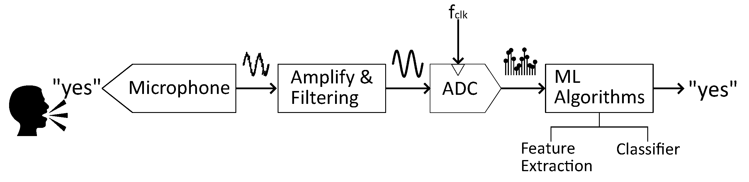
Figure 2.
General architecture of the Proposed KWS system.
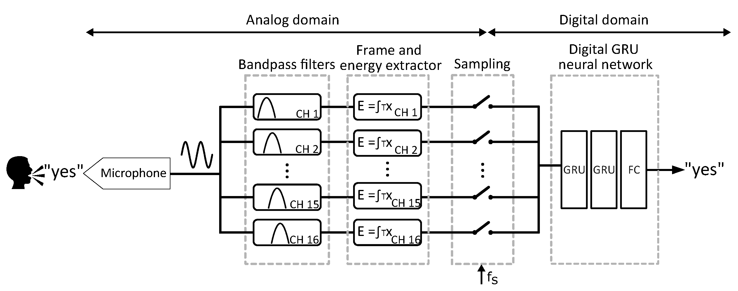
Figure 3.
General scheme of the analog feature extraction stage.
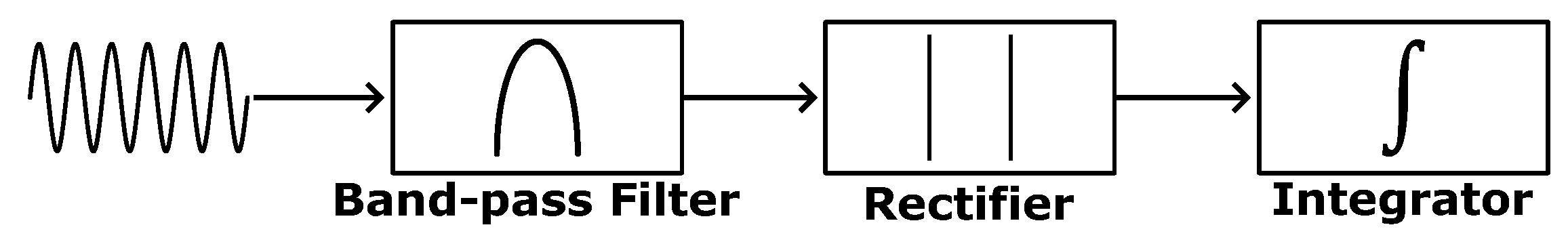
Figure 4.
Frequency response of the analog band-pass filter bank in logarithmic (top) and linear scales (bottom).
Figure 4.
Frequency response of the analog band-pass filter bank in logarithmic (top) and linear scales (bottom).
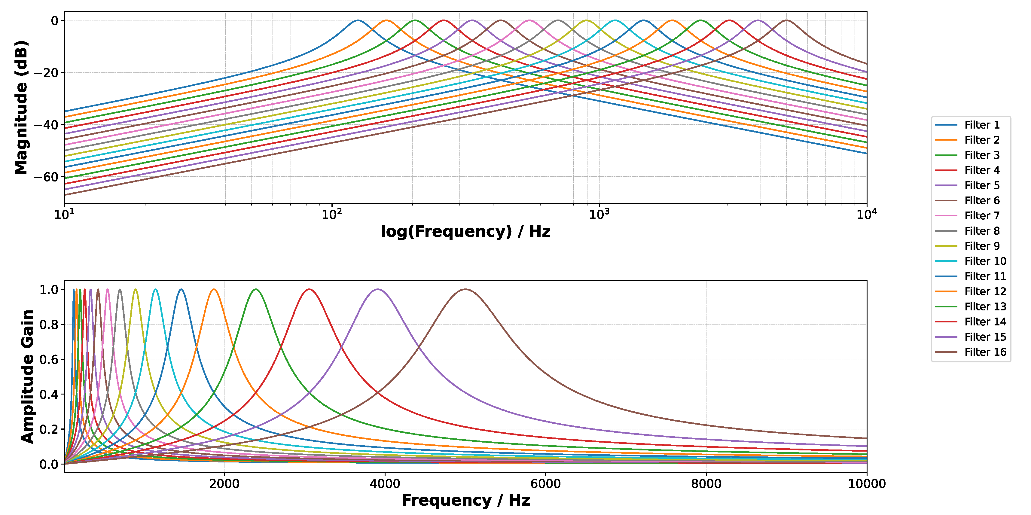
Figure 5.
Feature extraction using the keyword "yes" as an example. (a) Heatmap of the extracted features, representing the averaged rectified amplitude per frame. (b) Comparison between original audio wave and filtered wave for some selected filter channels.
Figure 5.
Feature extraction using the keyword "yes" as an example. (a) Heatmap of the extracted features, representing the averaged rectified amplitude per frame. (b) Comparison between original audio wave and filtered wave for some selected filter channels.
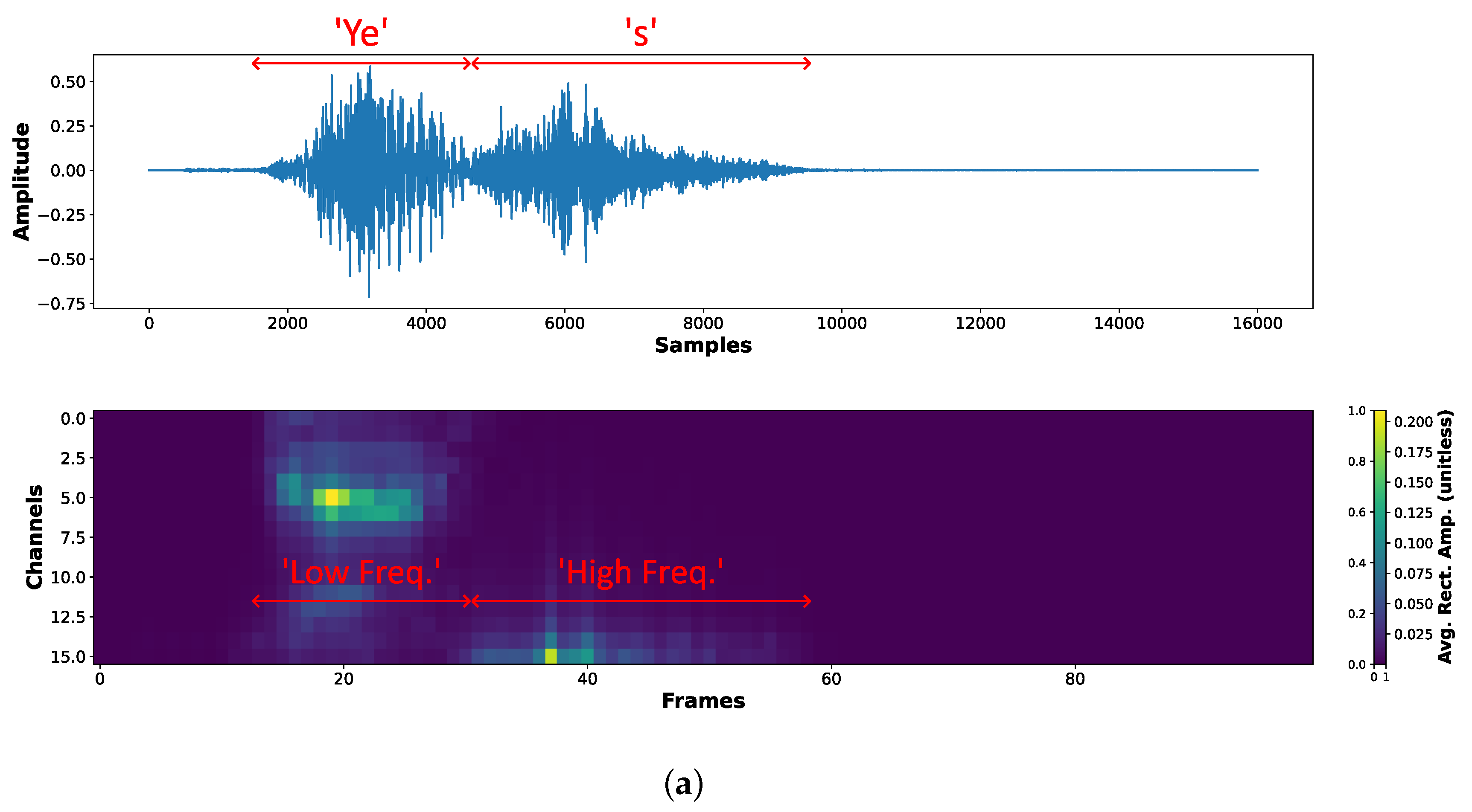
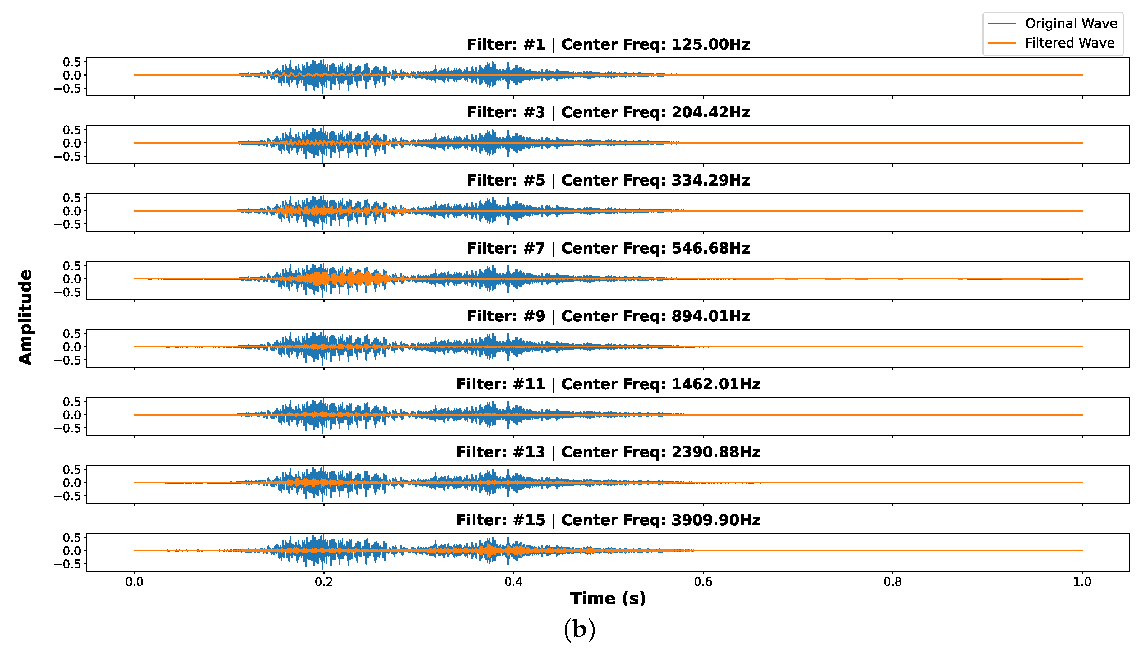
Figure 6.
Accuracy on GSCDv2 test set for different number units per GRU layer, and number of GRU hidden layers. Other hyperparameters are kept the same during training. () Different number of units per GRU layer, number of layers are set to 2. () Different GRU layers, number of units is fixed to 80.
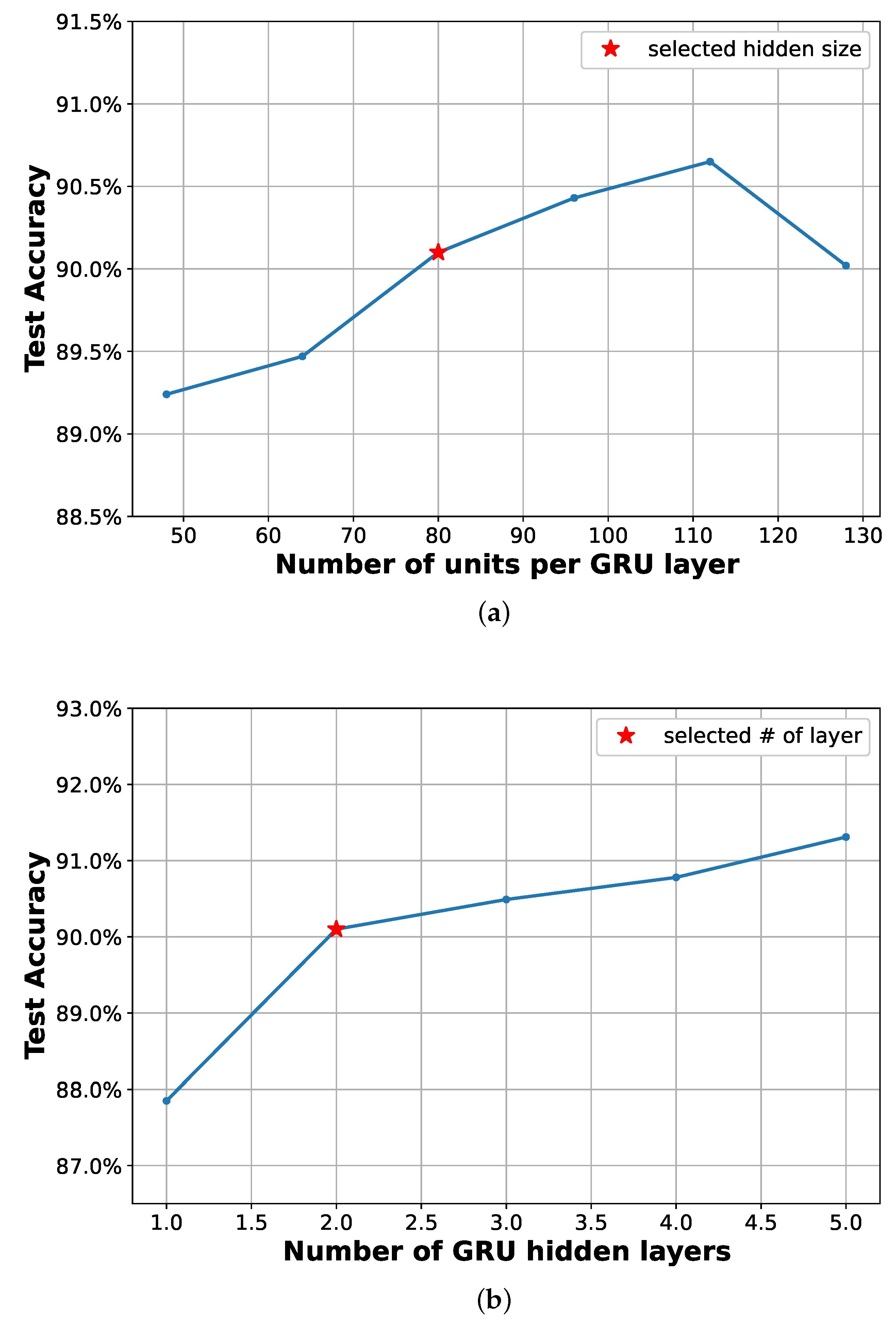
Figure 7.
LSQ-based QAT data flow in our GRU unit.
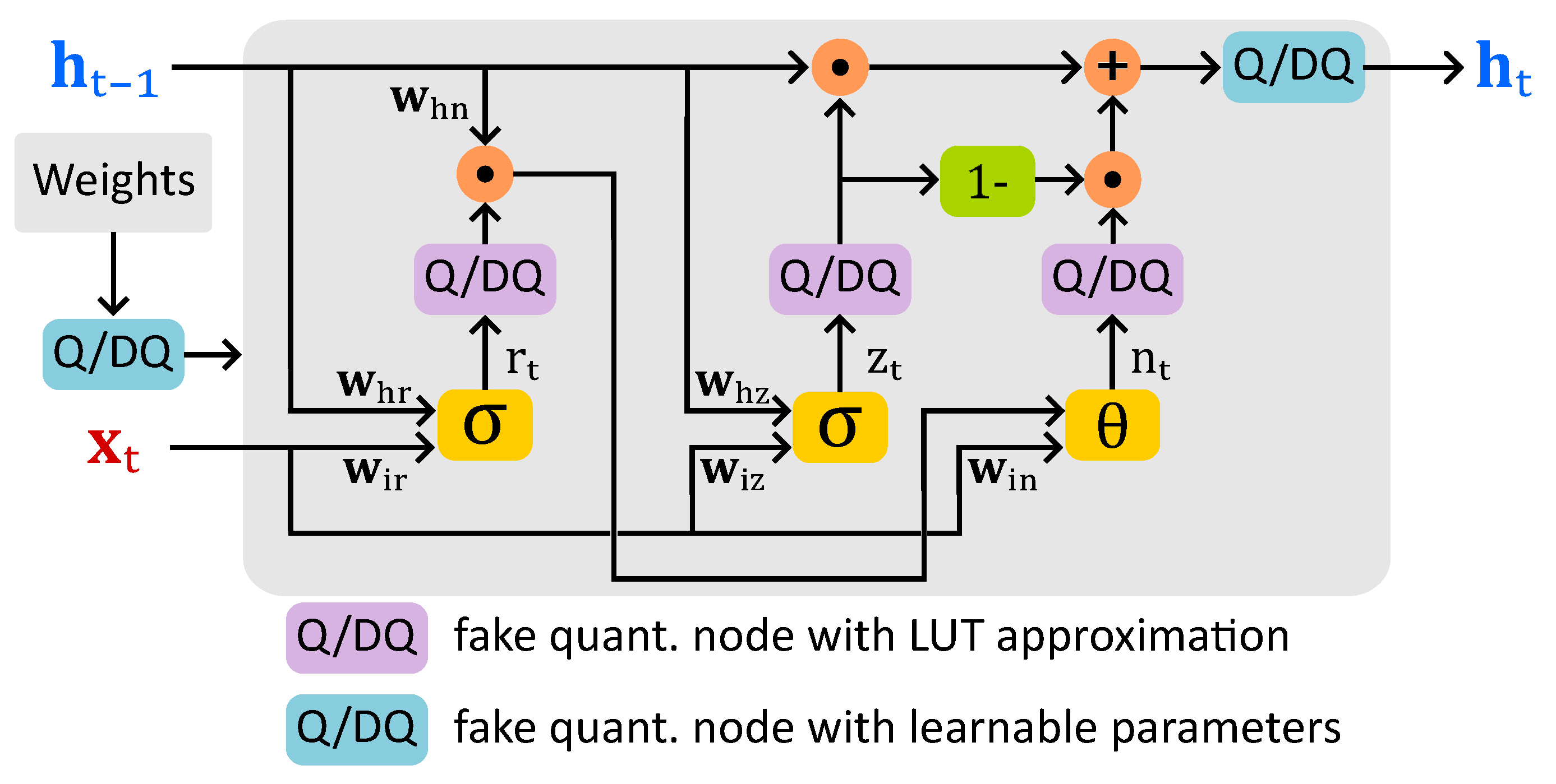
Figure 8.
QAT Data flow in our classifier with 2 GRU layers and 1 final fully connected (FC) layer.
Figure 9.
True positive rate (TPR) confusion matrix of our model on the 12-classes.

Table 1.
State-of-the-Art comparison.
| Villamizar TCASI’21[34] |
Kim JSSC’22[11] |
Yang JSSC’23[14] |
Mostafa ISSCC’24[9] |
Chen TCASAI’24[13] |
This work |
|
|---|---|---|---|---|---|---|
| Feature Ex. | Analog | Analog | Digital | Analog | Digital | Analog1 |
| # Channels | 32 | 16 | 26 | 16 | 10 | 16 |
| Classifier | Li-GRU2 | GRU | Skip RNN | GRU2 | Delta RNN | GRU3 |
| # RNN layers | - | 2 | 1 | 2 | 1 | 2 |
| Units / layer | - | 48 | 64 | 128 | 64 | 80 |
| NN Quant. | - | 8b w, 14b acti. | 8b w, 12b acti. | - | 8b w, - acti. | 4b w, 8b acti. |
| NN Memory (kB) | - | 24 | 18 | - | 24 | 34.84 |
| Dataset | GSCDv2 | GSCDv2 | GSCDv1 | GSCDv2 | GSCDv2 | GSCDv2 |
| # Classes (# KWs) | 12 (10) | 12 (10) | 7 (5) | 10 (10) | 12 (10) | 12 (10) |
| Accuracy (%) | 92.10% | 86.03% | 92.80% | 91.00% | 89.50% | 91.35% |
1 Transfer function-based software model, others are silicon-based measurements. 2 Off-chip software model w/o quantization. 3 Software model w/ LSQ and LUT-aware quantization. 4 Estimated memory size.
Disclaimer/Publisher’s Note: The statements, opinions and data contained in all publications are solely those of the individual author(s) and contributor(s) and not of MDPI and/or the editor(s). MDPI and/or the editor(s) disclaim responsibility for any injury to people or property resulting from any ideas, methods, instructions or products referred to in the content. |
© 2025 by the authors. Licensee MDPI, Basel, Switzerland. This article is an open access article distributed under the terms and conditions of the Creative Commons Attribution (CC BY) license (http://creativecommons.org/licenses/by/4.0/).
Copyright: This open access article is published under a Creative Commons CC BY 4.0 license, which permit the free download, distribution, and reuse, provided that the author and preprint are cited in any reuse.


