Submitted:
06 March 2025
Posted:
06 March 2025
Read the latest preprint version here
Abstract
As the most potential new reflective display technology, electrowetting display (EWD) has the advantages of simple structure, fast response, high contrast and rich colors. However, due to the hysteresis effect, gray-scales of EWD cannot be accurately controlled, which seriously restricts the industrialization process of this technology. In this paper, the oil movement process in an EWD pixel cell was simulated, and the influence of oil viscosity on hysteresis effect was studied based on the proposed simulation model. Firstly, the cause of hysteresis effect was analyzed through hysteresis curve of EWD. Then, based on COMSOL Multiphysics simulation environment, the oil movement process in an EWD pixel cell was simulated by coupling the phase field of laminar two-phase flow and electrostatic field. Finally, based on the simulation model, the influence of oil viscosity on hysteresis effect in an EWD pixel cell was studied. The experimental results showed that the maximum hysteresis difference of hysteresis effect increased with the increase of oil viscosity, and decreased with the decrease of oil viscosity. The oil viscosity had little effect on the maximum aperture ratio of EWD. The pixel on response time and pixel off response time increased with the increase of oil viscosity.
Keywords:
electrowetting display (EWD)
; hysteresis effect
; oil viscosity
; simulation
; contact angle hysteresis (CAH)
1. Introduction
The optical switch of electrowetting display (EWD) technology is realized by controlling the contraction and spread of colored oil in pixel cells [1]. The principle that the contact angle between liquid and solid interface changes after applying voltage has been applied in many aspects, such as lab-on-a-chip [2], micro zoom lens [3], energy collection [4]. Among them, EWD is the most promising application [5]. EWD technology has the characteristics of simple structure, fast response, high reflectivity, high contrast and rich colors [6]. Compared with the existing display technologies, it shows great advantages. However, due to the rough surface of pixel structure and the viscous resistance of oil-water interface, the hysteresis effect will appear during the pixel driving process [7,8]. As a result, gray-scales of EWD cannot be accurately controlled. In order to reduce the hysteresis effect, many scholars have made a lot of efforts.
The hysteresis effect of EWD refers to the difference of optical response during the driving process of pixel switch [9]. It was first discovered in 2006 by Van Dijk R of Liquavista when he improved the EWD to display video content with 4 bits of gray-scales and a resolution of 170 ppi [10]. In 2012, a hysteresis-free pixel switching structure was designed by adding hydrophilic patches or staircases [11]. The hysteresis effect could be better eliminated by this method, but it would reduce the aperture ratio of pixels and bring unpredictable difficulties to the manufacturing process. In the same year, electrowetting process of electrolyte drops on smooth and rough surfaces was studied by using the Lattice Boltzmann model [12]. It was observed that the hysteresis and saturation of contact angle were more obvious on the rough surface. In 2015, a theoretical model was proposed to describe the evolution of electrowetting on substrates with contact angle hysteresis, and the relationship between the apparent contact angle, voltage and other parameters were quantified [13]. The results showed that the theory and equation based on energy balance could successfully describe the electrowetting response with obvious contact angle hysteresis. In 2017, a method and principle for improving contact angle hysteresis was given based on the improved Young’s equation [14]. The relationship between lens focal length and applied voltage was studied by using three kinds of oil with different viscosity ratio as insulating liquid. The results showed that the focal length hysteresis could be reduced by reducing the oil viscosity. In 2020, a pixel structure was proposed for achieving accurate control of oil rupture position and move direction by adding additional pinning structures or spacing arrays [15,16]. This scheme could effectively reduce the hysteresis effect of EWD.
In order to reduce the hysteresis effect by changing the oil viscosity, based on COMSOL Multiphysics simulation environment, the oil movement process in a pixel cell was successfully simulated by coupling the laminar two-phase flow phase field and electrostatic field, and the influence of oil viscosity on the hysteresis effect in EWD was studied based on the proposed simulation model.
Principles of Hysteresis Effect in EWDs
The introduction should briefly place the study in a broad context and highlight why it is important. It should define the purpose of the work and its significance. The current state of the research field should be carefully reviewed and key publications cited. Please highlight controversial and diverging hypotheses when necessary. Finally, briefly mention the main aim of the work and highlight the principal conclusions. As far as possible, please keep the introduction comprehensible to scientists outside your particular field of research. References should be numbered in order of appearance and indicated by a numeral or numerals in square brackets—e.g., [1] or [2,3], or [4,5,6]. See the end of the document for further details on references.
2. Materials and Methods
2.1. Driving Principle of EWDs
An EWD panel is mainly composed of glass substrate, indium tin oxides (ITO) electrode, hydrophobic insulation layer (HIL), pixel wall, colored oil, polar liquid, and top plate [5,15], as shown in Figure 1. VG1 and VG2 are the gate signals of TFT1 and TFT2 respectively, which are used to control whether the source voltage VS charges the storage capacitor CS. When VG1 is at low level, TFT1 is off, and the voltage on CS1 is 0. At this time, without external voltage, the colored oil in pixels spreads naturally and covers the whole pixel, and the color of oil is displayed. When VG2 is at high level, TFT2 is on, and the voltage on CS2 is VS. At this time, the colored oil in pixels is pushed to a corner, and the color of the substrate is displayed. The contraction degree of oil is controlled by the applied voltage to achieve the purpose of displaying gray-scales.
Research manuscripts reporting large datasets that are deposited in a publicly available database should specify where the data have been deposited and provide the relevant accession numbers. If the accession numbers have not yet been obtained at the time of submission, please state that they will be provided during review. They must be provided prior to publication.
The different degrees of oil contraction represent different optical states, which are characterized by the aperture ratio. The aperture ratio is a proportion of oil opening area in a whole pixel [17]. The formula is defined as Equation (1).
In Equation (1), represents the aperture ratio, and represent the surface area of oil in a pixel and the surface area of a whole pixel respectively, represents the driving voltage applied to EWDs, and the area of pixel wall can be ignored in calculating the aperture ratio. The pixel wall is a transparent grid structure which can divide an EWD into several pixels.
2.2. Hysteresis Effect of EWDs
As shown in Figure 2, it is the relationship between driving voltage and aperture ratio when the conventional square wave is used to drive an EWD panel. The blue curve is the driving voltage rising stage, and the red curve is the driving voltage falling stage. It can be seen that there is a significant difference in the aperture ratio between the driving voltage rising stage and the driving voltage falling stage, that is, hysteresis effect. Generally, the absolute value of the aperture ratio difference under the same voltage value in the rising stage and the falling stage is called the hysteresis difference, and the aperture ratio curve formed in the rising stage and the falling stage is collectively called the hysteresis curve [18].
Combined with the morphological characteristics of hysteresis effect, through theoretical analysis and literature review [19,20,21,22], it can be seen that the main causes of hysteresis effect in EWD are the existence of oil rupture voltage, oil contact angle hysteresis, and oil contact angle saturation. The oil rupture voltage is caused by the fact that the electric field force is not enough to overcome the static friction and capillary force when the driving voltage is too low. Oil contact angle hysteresis is due to the inconsistency between oil forward contact angle and oil backward contact angle caused by dynamic friction and viscous resistance. Oil contact angle saturation is caused by the weakening of the electric field force due to charge trapping.
3. Numerical Methodology
The numerical method was realized by establishing and solving numerical equations. The purpose was to track the morphological changes and motion characteristics of the oil-water interface in the limited pixel cell under the action of external electric field force. In this paper, COMSOL Multiphysics simulation software was used to simulate the laminar two-phase flow under the action of electric field, and the laminar flow field was coupled with phase field and electrostatic field. The finite element method (FEM) was used to solve all governing equations, including Cahn-Hilliard equation, Laplace equation and Navier-Stokes equation. First, the Maxwell stress tensor equation was solved by adding an electrostatic field module, and the electric field force output from the electrostatic field module was fed back to the hydrodynamic module. Then, the Navier-Stokes equation and phase field equation were solved by the hydrodynamics module according to the specified fluid boundary conditions and the solution results of electrostatic field.
3.1. Governing Equations
The numerical method was realized by establishing and solving numerical equations. The purpose was to track the morphological changes and motion characteristics of the oil-water interface in the limited pixel cell under the action of external electric field force. In this paper, COMSOL Multiphysics simulation software was used to simulate the laminar two-phase flow under the action of electric field, and the laminar flow field was coupled with phase field and electrostatic field. The finite element method (FEM) was used to solve all governing equations, including Cahn-Hilliard equation, Laplace equation and Navier-Stokes equation. First, the Maxwell stress tensor equation was solved by adding an electrostatic field module, and the electric field force output from the electrostatic field module was fed back to the hydrodynamic module. Then, the Navier-Stokes equation and phase field equation were solved by the hydrodynamics module according to the specified fluid boundary conditions and the solution results of electrostatic field.
There are two kinds of fluids in EWD pixel cells, water and oil. During calculations, the fluids are assumed to be an incompressible and incompatible Newtonian fluid, and there are no chemical reactions in the flow process. The Navier-Stokes equation with momentum conservation and the continuum equation with mass conservation are used to describe the laminar flow field [23]. The governing equations are as follows:
Where, is the fluid velocity, is the fluid pressure, is the fluid density, is the hydrodynamic viscosity. And each item corresponds to inertial force, pressure, viscous force and external force acting on the fluid. The external force is mainly composed of surface tension, gravity and volume force. represents surface tension (N/m3), represents gravitational acceleration (m/s2), is the volume force (N/m3).
The fluid flow in EWD system is laminar flow (), and there is no diffusion effect between the two fluids. Moreover, the gravity can be ignored (). Therefore, electrostatic field force is the main factor causing fluid flow [24]. The parameters requiring coupling are the volume force and the surface tension caused by the applied electric field. The electrostatic volume force (N/m3) can be expressed by the divergence of Maxwell stress tensor [24].
The Maxwell stress tensor can be expressed as Equation (5).
Where, is the identity matrix, is the electric field, and is the potential shift field.
In the two-dimensional structural model, Maxwell stress tensor can be expressed as Equation (8).
The stress tensor in each direction can be obtained by substituting the parameters.
The change of volume force caused by electrostatic field only occurs at the interface of two-phase fluid, and its derivative can be obtained.
After an electric field is applied, the contact angle of three-phase contact line will be changed by the Maxwell stress. The contact angle refers to the external angle during the movement of water on the hydrophobic insulation layer, which is expressed by Lippmann-Young equation [9]. As shown in Equation (11), where, is the contact angle when the driving voltage is , and is the contact angle when the driving voltage is , and respectively represent the vacuum dielectric constant and the relative dielectric constant of the dielectric layer. And is the thickness of the dielectric layer, is the liquid-gas contact line.
For two-phase fluid movement, volume function method (VOF), level set method or phase field method are usually used to track the oil-water interface [25,26]. Based on the diffusion interface model, the phase field method characterizes the interface evolution of the system through the changes of order parameters and concentration field. In the phase field theory framework of COMSOL, the comprehensive action of physical interface motion and chemical potential change is expressed by differential equation, so as to the instantaneous change of interface is obtained. The phase field method does not directly track the change of the interface, but through the phase field variable describe fluid distance phase interface . In the region of two fluids, the phase field variable will be taken as , while in the transition region of the interface, the phase field variable changes smoothly between and . The oil-water interface is defined as a diffusion interface, the change of the oil-water interface is described by Cahn-Hilliard convection equation, and the phase field variables are obtained by solving the phase field equation [27,28,29]. The phase field governing equations are as follows:
Where, is the energy density (N), is the capillary width varying with the interface thickness (m). These two parameters and the surface tension coefficient (N/m) are described by Equation (14). is the mobility parameter, and the relation function between and is , is the mobility adjustment parameter. The phase field variable is expressed as in oil and in water. In order to correctly couple electrostatic field and laminar flow field, it is necessary to track the dielectric constant, density and viscosity between diffusion interfaces. The calculation formulas are as follows:
Where, , and represent the density, viscosity and dielectric constant of the fluid respectively. The average curvature between two liquid interfaces is calculated as follows [29]:
Where, and represent mean curvature and chemical potential energy respectively.
3.2. Boundary Conditions
The boundary conditions were the precondition that the governing equations had a definite solution on the boundary of the region [30]. The size of the pixel cell used in the calculation domain was shown in Figure 3(a), and the relevant boundary conditions were shown in Figure 3(b).
In the EWD structure model, zero-charge boundary conditions were set around the model, that’s, . This also meant that no displacement field could penetrate the boundary at the surrounding inner boundary, and the potential was discontinuous at the boundary. For electrostatic field boundary conditions, the potential Vapp and grounding boundary conditions should also be specified. And wetted wall, initial interface, inlet and outlet were need to be set for the phase field boundary conditions. The wetted wall boundary conditions were determined by Equation (20) and Equation (21).
In the initial interface boundary condition, the two-phase flow contact interface was selected as the position of the initial interface, . Both sides of the fluid of the EWDs were selected as the inlet and outlet boundary conditions, which were set as the outlet end in the actual simulation process, and the pressure constraint term was set at the end point. In addition, the initial value of volume force and velocity should be set, and the initial value of velocity was set to 0 (m/s).

Table 1.
Material, geometric and interfacial parameters of the proposed model.
| Parameters | Quantity | Symbol | Value | Unit |
|---|---|---|---|---|
| Material | density of oil | 880 | kg/m³ | |
| density of water | 998 | kg/m³ | ||
| dynamic viscosity of oil | 0.002 | Pa·s | ||
| dynamic viscosity of water | 0.001 | Pa·s | ||
| dielectric constant of oil | 2.2 | 1 | ||
| dielectric constant of water | 80 | 1 | ||
| dielectric constant of hydrophobic insulating layer | 1.95 | 1 | ||
| dielectric constant of pixel wall | 3.28 | 1 | ||
| Geometric | width of pixel cell | 150 | μm | |
| height of pixel wall | 5.6 | μm | ||
| width of pixel wall | 15 | μm | ||
| thickness of hydrophobic insulating layer | 1 | μm | ||
| thickness of oil | 5.6 | μm | ||
| Interfacial | surface tension of oil and water | 0.015 | N/m | |
| contact angle of pixel wall | 65 | deg | ||
| contact angle of hydrophobic insulating layer | 150 | deg | ||
| contact angle of top plate | 90 | deg |
4. Experimental Results and Discussion
The oil movement process in an EWD pixel cell was successfully simulated by the established simulation model. Therefore, based on this model, the influence of oil viscosity on the performance of EWD can be investigated through experiments, including response time, maximum aperture ratio and hysteresis effect. In experiments, the dynamic viscosity coefficient was used to characterize the oil viscosity, and the influence of oil viscosity on the hysteresis effect of the EWD was emphatically analyzed. All parameters were kept constant and the temperature was kept at 25℃. Segment function was used to describe the driving waveform, and the driving voltage ranged from 0V to 30V. The dynamic viscosity coefficient was dynamically changed and the corresponding aperture ratio data were recorded.
According to Equation (1), the formula for calculating the aperture ratio in a two-dimensional model can be obtained. Assume that the pixel cell is square and the side length is . The contact surface between the oil and the hydrophobic insulating layer is round, with a diameter of . Then the calculation formula of the aperture ratio in the two-dimensional model can be obtained. The specific description is as follows, is the rupture voltage.
The oil movement process can be divided into an opening stage after applying the external voltage and a closing stage after removing the external voltage. A segment function was used to describe the traditional square wave, as shown in Figure 4(a). Based on the established simulation model, the simulation of an entire oil movement process, including an opening stage and a closing stage can be realized. As shown in Figure 4(b) and Figure 4(c), it was a simulation of the oil movement process in a EWD pixel cell. When , an external voltage of 30V was applied, and the oil started to contract under the action of electric field force. At , the oil started to break away from the pixel wall, showing an opening. At , the opening reached the maximum value. At this point, the oil opening process was completed. When , the applied external voltage was removed, and the oil began to spread under the effect of surface tension. When , the oil was closed and completely contacts the pixel wall. At this point, the oil closing process was completed.
4.1. Influence of Oil Viscosity on Response Time
In the experiment, a 30V driving voltage was applied first and removed after the oil was completely opened. During this process, the pixel on response time and the pixel off response time were recorded when the oil was fully opened and fully closed under different oil dynamic viscosity coefficient. The relationship between oil dynamic viscosity coefficient and pixel response time could be obtained, as shown in Figure 5. In the figure, the blue curve was pixel on response time curve, the red curve was pixel off response time curve, and the green curve indicated that the pixel could not be opened within 16ms. It can be seen that the pixel on response time and pixel off response time increased with the increase of oil dynamic viscosity coefficient. This was because the increase of oil dynamic viscosity would increase the viscosity resistance.
4.2. Influence of Oil Viscosity on Maximum Aperture Ratio
In the experiment, a 30V driving voltage was applied. During this process, the maximum aperture ratio of a pixel cell under different oil dynamic viscosity coefficient was recorded when the oil was fully opened. The relationship between the oil dynamic viscosity coefficient and the maximum aperture ratio of a pixel cell could be obtained, as shown in Figure 6. The blue curve was the maximum aperture ratio curve of a pixel, and the red curve indicated that the pixel could not be opened within 16ms. It can be seen that the maximum aperture ratio of a pixel cell was very close, indicating that the change of oil dynamic viscosity could not change the maximum aperture ratio of a pixel cell.
4.3. Influence of Oil Viscosity on Hysteresis Effect
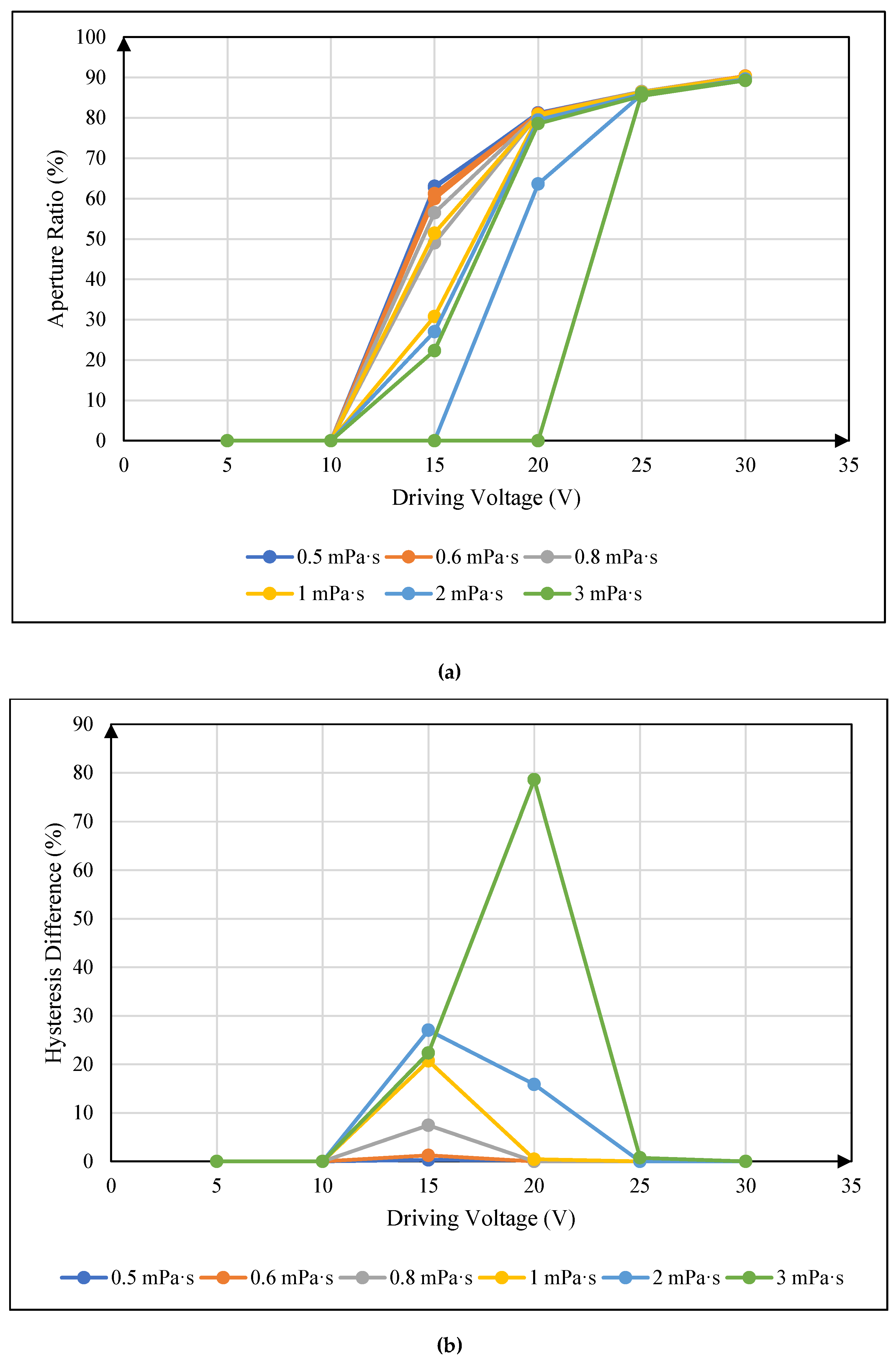
The dynamic viscosity coefficient of oil commonly used in the preparation of EWDs is 2 mPa ∙ s. In the experiment, the traditional square wave was used to drive a pixel cell, and the hysteresis curves under different dynamic viscosity systems were recorded. The relationship between oil dynamic viscosity coefficient and hysteresis curve could be obtained, as shown in Figure 7(a). In order to more intuitively reflect the relationship between oil dynamic viscosity coefficient and hysteresis effect, the data of aperture ratio in the experimental results were further processed. The absolute value of the difference of the aperture ratio under the same voltage during the rising and falling process was defined as the hysteresis difference. The relationship between oil dynamic viscosity coefficient and hysteresis difference curve could be obtained, as shown in Figure 7(b).
It can be seen from Figure 7 that during the movement of the oil in a pixel cell, the hysteresis difference first increases and then decreases with the increase of the driving voltage, forming a maximum hysteresis difference in this process, indicating the degree of hysteresis effect. The maximum hysteresis value decreases with the increase of oil dynamic viscosity coefficient, indicating that oil dynamic viscosity coefficient is positively correlated with hysteresis effect. This is because the increase of oil viscosity will cause the increase of shear stress during oil movement, that is, the increase of viscosity resistance. Greater viscous resistance will consume more electric field force to do work, resulting in the change of effective work done by the same electric field force during oil movement.
5. Conclusions
In summary, based on COMSOL Multiphysics simulation environment, the driving process of hysteresis effect in an electrowetting display pixel cell was successfully simulated by coupling the laminar two-phase flow phase field and electrostatic field. Based on the proposed simulation model, the influence of oil viscosity on hysteresis effect of electrowetting display was studied. The experimental results showed that the maximum hysteresis difference of hysteresis effect increased with the increase of oil viscosity, and decreased with the decrease of oil viscosity. The oil viscosity had little effect on the maximum aperture ratio of EWD. The pixel on response time and pixel off response time increased with the increase of oil viscosity.
Author Contributions
Conceptualization, W.L., L.L. and L.W.; methodology, T.Z. and L.T.; validation, W.L., C.X. and J.L.; formal analysis, Z.Y.; writing—original draft preparation, W.L.; writing—review and editing, L.W. and Z.Y.; visualization, W.L.; supervision, G.Z.; funding acquisition, G.Z. All authors have read and agreed to the published version of the manuscript.
Funding
This research was funded by National Key R&D Program of China (No. 2021YFB3600605), National Natural Science Foundation of China (U23A20368), the Program for Guangdong Innovative and Entrepreneurial Teams (No. 2019BT02C241), Guangdong Basic and Applied Basic Research Foundation (2023A1515010050), Guangdong Provincial Key Laboratory of Optical Information Materials and Technology (2023B1212060065), Guangzhou Key Laboratory of Electronic Paper Displays Materials and Devices (No. 201705030007) and the 111 Project.
Institutional Review Board Statement
Not applicable.
Data Availability Statement
All data are contained within the article.
Conflicts of Interest
The authors declare no conflicts of interest.
References
- Hayes, R.A.; Feenstra, B.J. Video-speed electronic paper based on electrowetting. Nature 2003, 425, 383–385. [Google Scholar] [CrossRef] [PubMed]
- Moon, H.; Wheeler, A.R.; Garrell, R.L.; Loo, J.A.; Kim, C.J. An integrated digital microfluidic chip for multiplexed proteomic sample preparation and analysis by MALDI-MS. Lab on a Chip 2006, 6, 1213–1219. [Google Scholar] [CrossRef]
- Berge, B.; Peseux, J. Variable focal lens controlled by an external voltage: An application of electrowetting. The European Physical Journal E 2000, 3, 159–163. [Google Scholar] [CrossRef]
- Krupenkin, T.; Taylor, J.A. Reverse electrowetting as a new approach to high-power energy harvesting. Nature communications 2011, 2, 1–8. [Google Scholar] [CrossRef]
- Li, W.; Wang, L.; Zhang, T.; Lai, S.; Liu, L.; He, W.; Yi, Z. Driving Waveform Design with Rising Gradient and Sawtooth Wave of Electrowetting Displays for Ultra-Low Power Consumption. Micromachines 2020, 11, 145. [Google Scholar] [CrossRef]
- Yi, Z.; Huang, Z.; Lai, S.; He, W.; Wang, L.; Chi, F.; Zhang, C.; Shui, L.; Zhou, G. Driving Waveform Design of Electrowetting Displays Based on an Exponential Function for a Stable Grayscale and a Short Driving Time. Micromachines 2020, 11, 313. [Google Scholar] [CrossRef]
- Ku, Y.S.; Kuo, S.W.; Tsai, Y.H.; Cheng, P.P.; Chen, J.L.; Lan, K.W.; Cheng, W.Y. The Structure and Manufacturing Process of Large Area Transparent Electrowetting Display. SID Symposium Digest of Technical Papers 2012, 43, 850–852. [Google Scholar] [CrossRef]
- Sun, B.; Heikenfeld, J. Observation and optical implications of oil dewetting patterns in electrowetting displays. Journal of Micromechanics and Microengineering 2008, 18, 025027. [Google Scholar] [CrossRef]
- Yi, Z.; Feng, W.; Wang, L.; Liu, L.; Lin, Y.; He, W.; Zhou, G. Aperture Ratio Improvement by Optimizing the Voltage Slope and Reverse Pulse in the Driving Waveform for Electrowetting Displays. Micromachines 2019, 10, 862. [Google Scholar] [CrossRef]
- Van, Dijk.R.; Feenstra, B.J.; Hayes, R.A.; Camps, I.G.J.; Boom, R.G.H.; Wagemans, M.M.H.; Feil, H. Gray scales for video applications on electrowetting displays. SID Symposium Digest of Technical Papers 2006, 37, 1926–1929. [Google Scholar] [CrossRef]
- Giraldo, A.; Vermeulen, P.; Figura, D.; Spreafico, M.; Meeusen, J.A.; Hampton, M.W.; Novoselov, P. Improved Oil Motion Control and Hysteresis-Free Pixel Switching of Electrowetting Displays. In SID Symposium Digest of Technical Papers 2012, 42, 625–628. [Google Scholar] [CrossRef]
- Li, H.; Fang, H. Hysteresis and saturation of contact angle in electrowetting on a dielectric simulated by the lattice Boltzmann method. Journal of adhesion science and technology 2012, 26, 1873–1881. [Google Scholar] [CrossRef]
- Rui, Z.; Qi-Chao, L.; Ping, W.; Zhong-Cheng, L. Contact angle hysteresis in electrowetting on dielectric. Chinese Physics B 2015, 24, 086801. [Google Scholar] [CrossRef]
- Zeng, Z.; Peng, R.; He, M. Effect of oil liquid viscosity on hysteresis in double-liquid variable-focus lens based on electrowetting. In International Conference on Optical and Photonics Engineering 2017, 10250, 212–216. [Google Scholar] [CrossRef]
- Dou, Y.; Tang, B.; Groenewold, J.; Li, F.; Yue, Q.; Zhou, R.; Zhou, G. Oil motion control by an extra pinning structure in electro-fluidic display. Sensors 2018, 18, 1114. [Google Scholar] [CrossRef]
- Dou, Y.; Chen, L.; Li, H.; Tang, B.; Henzen, A.; Zhou, G. Photolithography fabricated spacer arrays offering mechanical strengthening and oil motion control in electrowetting displays. Sensors 2020, 20, 494. [Google Scholar] [CrossRef]
- Zhang, X.M.; Bai, P.F.; Hayes, R.A.; Shui, L.L.; Jin, M.L.; Tang, B.; Zhou, G.F. Novel driving methods for manipulating oil motion in electrofluidic display pixels. Journal of Display Technology 2016, 12, 200–205. [Google Scholar] [CrossRef]
- Li, W.; Wang, L.; Henzen, A. A Multi Waveform Adaptive Driving Scheme for Reducing Hysteresis Effect of Electrowetting Displays. Frontiers in Physics 2020, 8, 618811. [Google Scholar] [CrossRef]
- Eral, H.B.; ’t Mannetje, D.J.C.M.; Oh, J.M. Contact angle hysteresis: a review of fundamentals and applications. Colloid and polymer science 2013, 291, 247–260. [Google Scholar] [CrossRef]
- Guo, Y.; Deng, Y.; Xu, B.; Henzen, A.; Hayes, R.; Tang, B.; Zhou, G. Asymmetrical Electrowetting on Dielectrics Induced by Charge Transfer through an Oil/Water Interface. Langmuir 2018, 34, 11943–11951. [Google Scholar] [CrossRef] [PubMed]
- Chang, J.H.; Pak, J.J. Effect of contact angle hysteresis on electrowetting threshold for droplet transport. Journal of adhesion science and technology 2012, 26, 2105–2111. [Google Scholar] [CrossRef]
- Quinn, A.; Sedev, R.; Ralston, J. Contact angle saturation in electrowetting. The journal of physical chemistry B 2005, 109, 6268–6275. [Google Scholar] [CrossRef] [PubMed]
- Arzpeyma, A.; Bhaseen, S.; Dolatabadi, A.; Wood-Adams, P. A coupled electro-hydrodynamic numerical modeling of droplet actuation by electrowetting. Colloids and Surfaces A: Physicochemical and Engineering Aspects 2008, 323, 28–35. [Google Scholar] [CrossRef]
- Hsieh, W.L.; Lin, C.H.; Lo, K.L.; Lee, K.C.; Cheng, W.Y.; Chen, K.C. 3D electrohydrodynamic simulation of electrowetting displays. Journal of Micromechanics and Microengineering 2014, 24, 125024. [Google Scholar] [CrossRef]
- Yurkiv, V.; Yarin, AL.; Mashayek, F. Modeling of Droplet Impact onto Polarized and Nonpolarized Dielectric Surfaces. Langmuir 2018, 34, 10169–10180. [Google Scholar] [CrossRef] [PubMed]
- Zhu, G.P.; Yao, J.; Zhang, L.; Sun, H.; Li, A.F.; Shams, B. Investigation of the Dynamic Contact Angle Using a Direct Numerical Simulation Method. Langmuir 2016, 32, 11736–11744. [Google Scholar] [CrossRef]
- Zhao, Q.; Tang, B.; Dong, B.; Li, H.; Zhou, R.; Guo, Y.; Dou, Y.; Deng, Y.; Groenewold, J.; Henzen, A.V.; Zhou, G. Electrowetting on dielectric: experimental and model study of oil conductivity on rupture voltage. Journal of Physics D Applied Physics 2018, 51, 195102. [Google Scholar] [CrossRef]
- Yue, P.T.; Feng, J.J.; Liu, C.; Shen, J. A diffuse-interface method for simulating two-phase flows of complex fluids. Journal of Fluid Mechanics 2004, 515, 293–317. [Google Scholar] [CrossRef]
- Cahn, J.W.; Hilliard, J.E. Free Energy of a Nonuniform System. I. Interfacial Free Energy. The Journal of Chemical Physics 1958, 28, 258–267. [Google Scholar] [CrossRef]
- Yang, G.; Zhuang, L.; Bai, P.; Tang, B.; Henzen, A.; Zhou, G. Modeling of Oil/Water Interfacial Dynamics in Three-Dimensional Bistable Electrowetting Display Pixels. ACS omega 2020, 5, 5326–5333. [Google Scholar] [CrossRef]
Figure 1.
The structure and driving principle of EWDs. The color of oil was displayed in a pixel when no external voltage was applied. And the color of substrate was displayed when the external voltage was applied.
Figure 1.
The structure and driving principle of EWDs. The color of oil was displayed in a pixel when no external voltage was applied. And the color of substrate was displayed when the external voltage was applied.
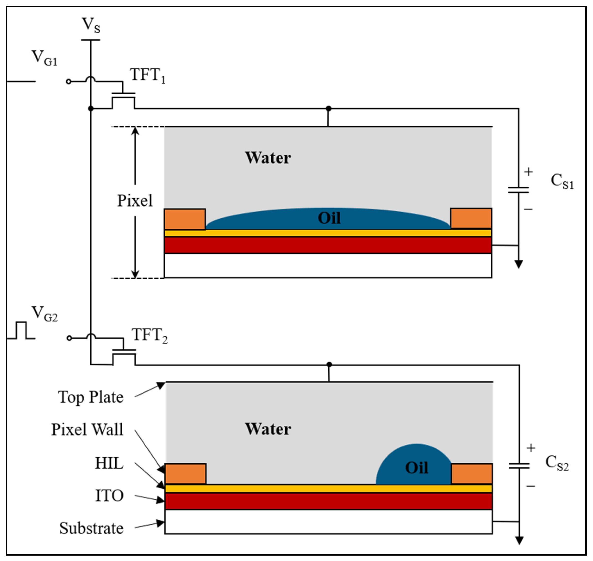
Figure 2.
Hysteresis curve of EWD driven by conventional square wave. The blue curve is the driving voltage rising stage, and the red curve is the driving voltage falling stage.
Figure 2.
Hysteresis curve of EWD driven by conventional square wave. The blue curve is the driving voltage rising stage, and the red curve is the driving voltage falling stage.
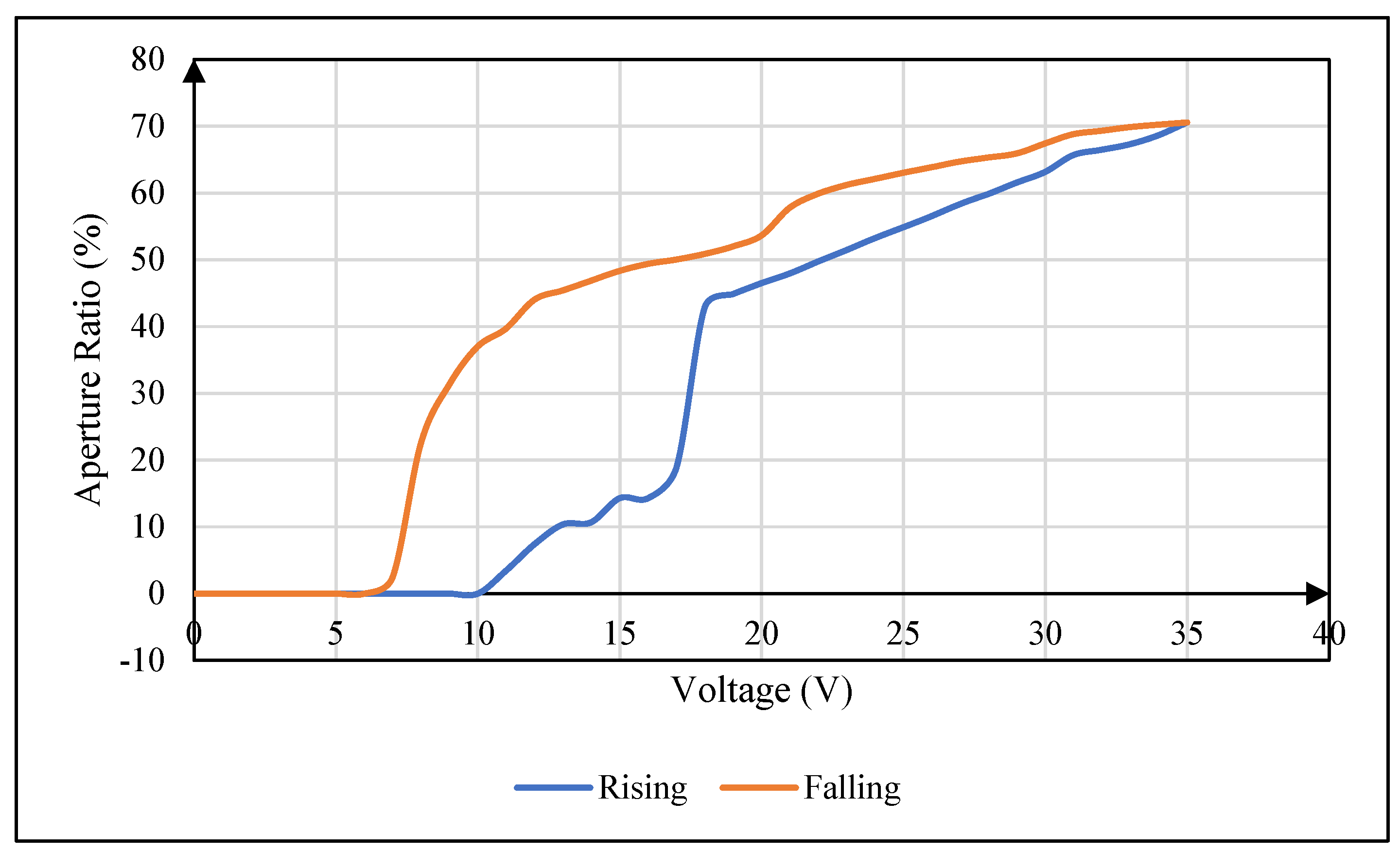
Figure 3.
Pixel cell size and relevant boundary conditions. (a) The size of pixel cell. (b) The relevant boundary conditions.
Figure 3.
Pixel cell size and relevant boundary conditions. (a) The size of pixel cell. (b) The relevant boundary conditions.
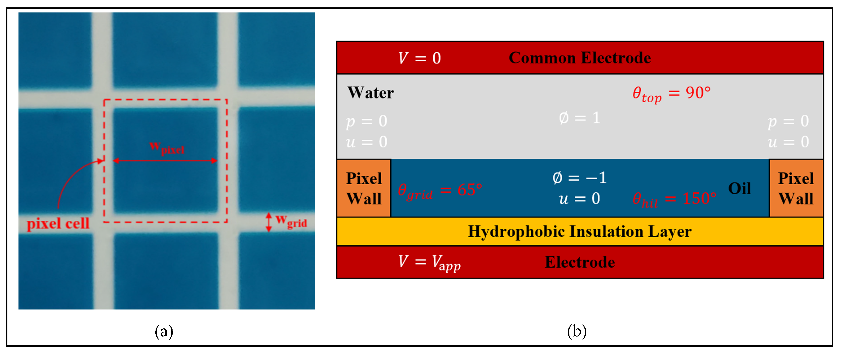
Figure 4.
Simulation of oil movement process in an EWD pixel cell. (a) Driving waveform used in the simulation. (b) Pixel on process. (c) Pixel off process.
Figure 4.
Simulation of oil movement process in an EWD pixel cell. (a) Driving waveform used in the simulation. (b) Pixel on process. (c) Pixel off process.
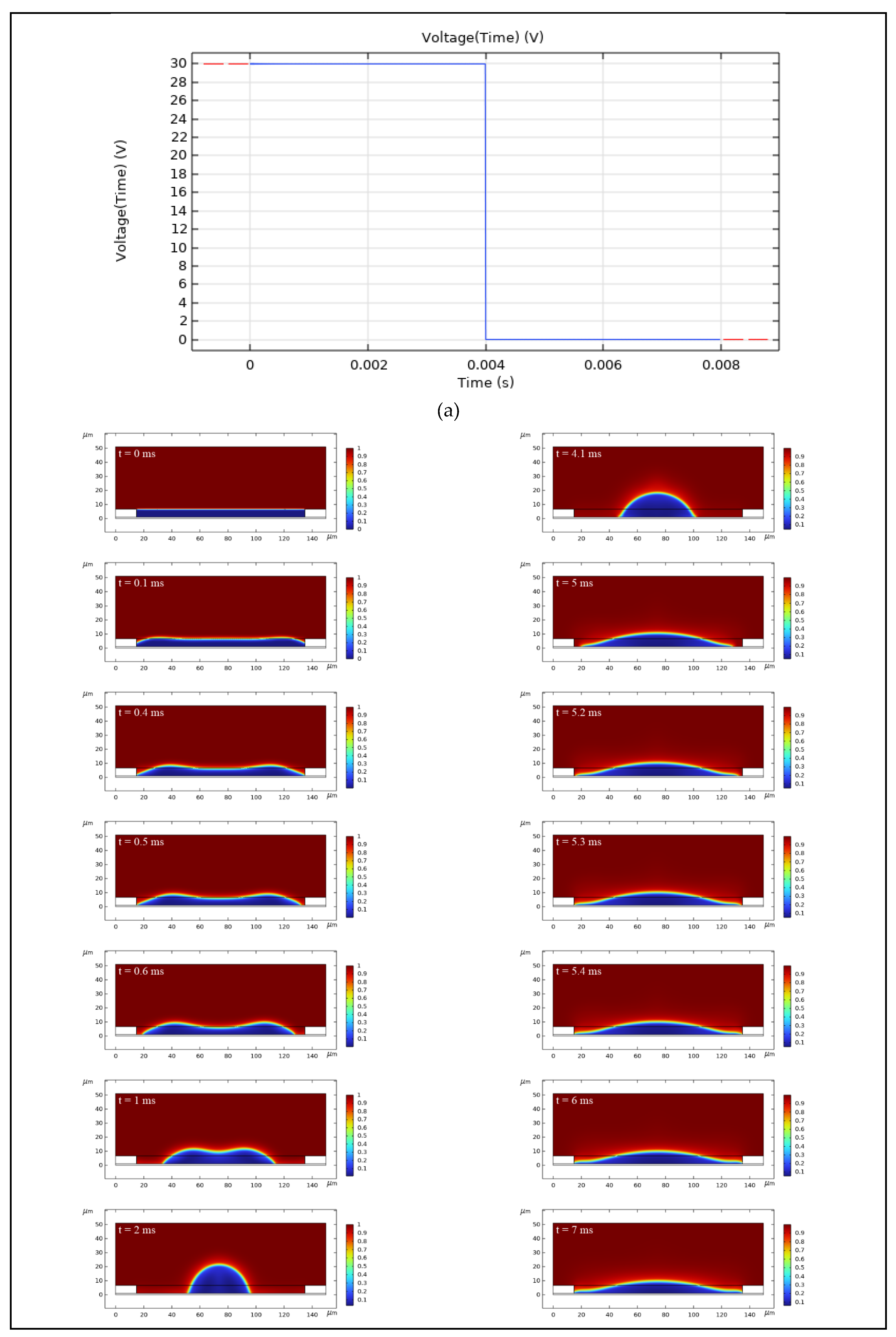
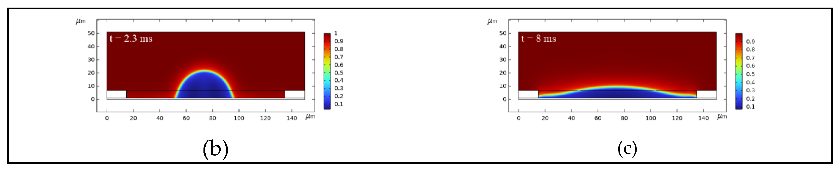
Figure 5.
The relationship between oil dynamic viscosity coefficient and pixel response time. The blue curve was pixel on response time curve, the red curve was pixel off response time curve, and the green curve indicated that the pixel could not be opened within 16ms.
Figure 5.
The relationship between oil dynamic viscosity coefficient and pixel response time. The blue curve was pixel on response time curve, the red curve was pixel off response time curve, and the green curve indicated that the pixel could not be opened within 16ms.
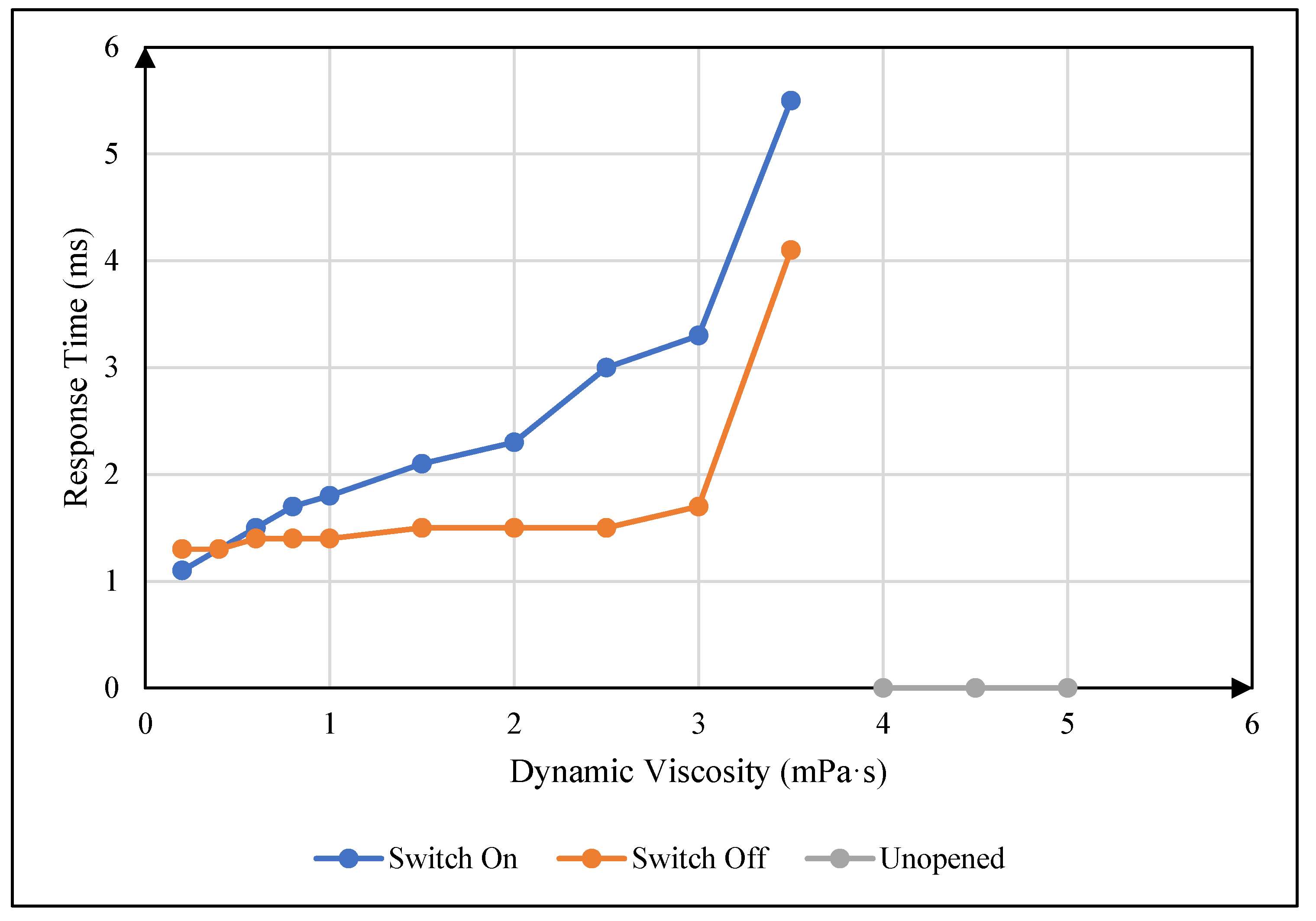
Figure 6.
The relationship between oil dynamic viscosity coefficient and maximum aperture ratio. The blue curve was the maximum aperture ratio curve of a pixel, and the red curve indicated that the pixel could not be opened within 16ms.
Figure 6.
The relationship between oil dynamic viscosity coefficient and maximum aperture ratio. The blue curve was the maximum aperture ratio curve of a pixel, and the red curve indicated that the pixel could not be opened within 16ms.
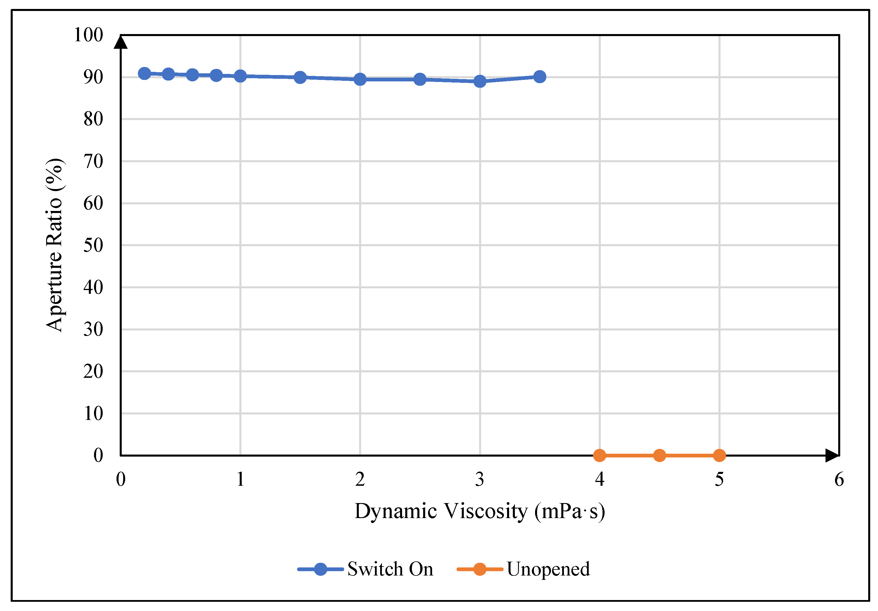
Figure 7.
The relationship between oil dynamic viscosity coefficient and pixel hysteresis effect. (a) The relationship between oil dynamic viscosity coefficient and hysteresis curve. (b) The relationship between oil dynamic viscosity coefficient and hysteresis difference.
Figure 7.
The relationship between oil dynamic viscosity coefficient and pixel hysteresis effect. (a) The relationship between oil dynamic viscosity coefficient and hysteresis curve. (b) The relationship between oil dynamic viscosity coefficient and hysteresis difference.
Disclaimer/Publisher’s Note: The statements, opinions and data contained in all publications are solely those of the individual author(s) and contributor(s) and not of MDPI and/or the editor(s). MDPI and/or the editor(s) disclaim responsibility for any injury to people or property resulting from any ideas, methods, instructions or products referred to in the content. |
© 2025 by the authors. Licensee MDPI, Basel, Switzerland. This article is an open access article distributed under the terms and conditions of the Creative Commons Attribution (CC BY) license (http://creativecommons.org/licenses/by/4.0/).
Copyright: This open access article is published under a Creative Commons CC BY 4.0 license, which permit the free download, distribution, and reuse, provided that the author and preprint are cited in any reuse.


