Submitted:
05 March 2025
Posted:
10 March 2025
You are already at the latest version
Abstract
To understand phase transition processes like solidification, phase field models are frequently employed. These models couple the energy (heat) equation for temperature with a nonlinear parabolic partial differential equation (p.d.e.) that includes a second unknown, the phase, which takes characteristic values, such as zero in the solid phase and one in the liquid phase. We consider a simplified phase field model described by a system of parabolic p.d.e’s, q(ϕ)ϕt = ∇ · (A(ϕ)∇ϕ) + f (ϕ, u), ut = Δu + [p(ϕ)]t, where ϕ(x, y, t) represents the phase indicator function and u(x, y, t) denotes the temperature. The functions q, p, and f are given scalars, and A is a 2×2 diagonal matrix dependent on ϕ. This system is posed for t ≥ 0 on a rectangle in the x, y plane with appropriate boundary and initial conditions. We solve the system using a finite difference method that uses for both equations the Crank-Nicolson-ADI scheme. We prove a convergence result for the method and show results of numerical experiments verifying its order of accuracy. The isotropic system is numerically solved using Crank-Nicolson-ADI finite difference discretization for both equations. The initial-boundary-value problem is considered with homogeneous Dirichlet boundary conditions for ϕ and u. The paper presents preliminary results on finite difference approximations, establishes the main result, showing that finite difference approximations to u and ϕ converge in the discrete L2 and H1 norms with bounds of order Δt2 + h2, given a stability condition of Δt h ≤ σ. Finally, numerical experiments confirm the convergence orders.
Keywords:
1. Introduction
2. The Problem
3. Notation and Preliminary Results
- a)
- Let Then
- b)
- Let Then
- c)
-
If then for
- i)
- ii)
- iii)
- iv)
- v)
4. Error Estimation
4.1. Local Error
4.2. Error Estimate
5. Numerical Verification of the Order of Convergence

| J | errors | order | errors | order |
| 50 | ||||
| 75 | ||||
| 112 | ||||
| 168 | ||||
| 252 | ||||
| 378 | ||||
| 567 | ||||
6. The Problem
7. Notation and Preliminary Results
- a)
- Let Then
- b)
- Let Then
- c)
-
If then for
- i)
- ii)
- iii)
- iv)
- v)
8. Error Estimation
8.1. Local Error
8.2. Error Estimate
9. Numerical Verification of the Order of Convergence
| J | errors | order | errors | order |
| 50 | ||||
| 75 | ||||
| 112 | ||||
| 168 | ||||
| 252 | ||||
| 378 | ||||
| 567 | ||||
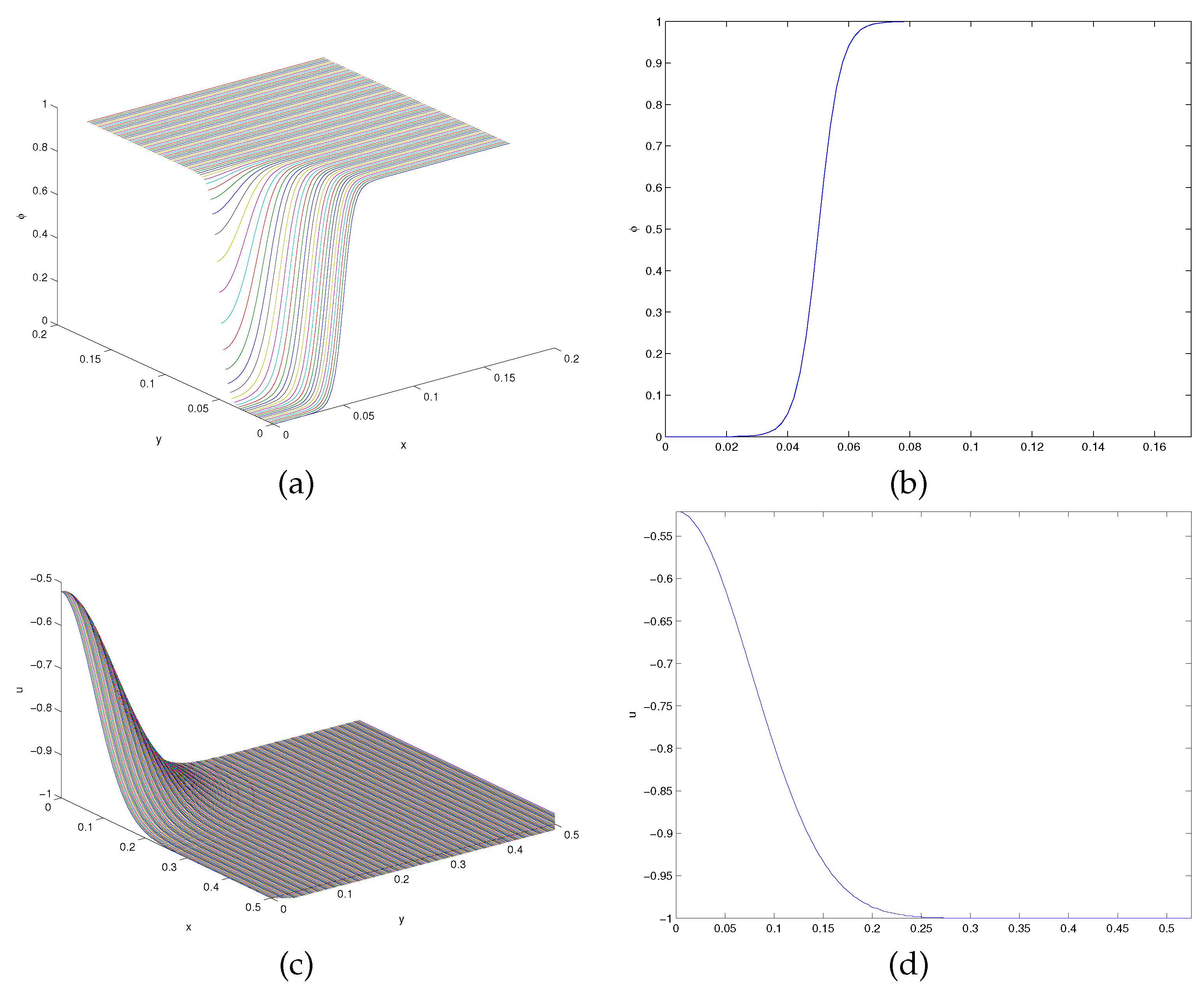
| (a) | (b) |
| (c) | (d) |
Acknowledgments
References
- B. Billia and R. Trevedi, “Pattern formation in crystal growth”, in M. E. Glicksman and S. P. Marsh, “The dendrite”, in Handbook of Crystal Growth, Vol. 1, ed. by D.T.J. Hurle, North-Holland, Amsterdam, 1993.
- E. Burman and J. Rappaz, “Existence of solutions to an anisotropic phase field model”, Mathematical Methods in the Applied Sciences, Vol. 26 (2003), pg. 1137-1160. [CrossRef]
- E. Burman, M. Picasso. and J. Rappaz, “Analysis and computation of dendritic growth in binary alloys using a phase-field model”, to appear in Proccedings of ENUMATH conference.
- E. Burman, D. Kessler, J.Rappaz, “Convergence of the finite element method applied to an anisotropic phase-field model”, Annales Math. B. Pascal, Vol. 11 (2004), pg. 69-95.
- J.E. Dendy, “Alternating direction methods for nonlinear time-depedent problems”, SIAM .I. Numer. Anal., Vol. 14 (1977), pg. 313-326.
- J.S. Langer, “Models of pattern formation in first-order phase transitions”, in Directions in Condensed Matter Physics, ed. By G. Grinsteil and G. Mazenko, World Scientific, Singapore 1986, pg. 164-186.
- N. Provatas, N. Goldenfeld, and J.A. Dantzig, "Efficient computation of dendritic microstructures using adaptive mesh refinement", Physical Review Letters, Vol. 80 (1998), pp. 3308-3311. [CrossRef]
- Chr. A. Sfyrakis and V. A. Dougalis, “A fast numerical method for a simplified phase field model”, in Mathematical Methods in Scattering Theory and Biomedical Engineering, ed. by World Sci. Publ., Hackensack, NJ, 2006, pg.208–215.
- Chr. A. Sfyrakis, “Mathematical and numerical models for materials phase change problems”, Ph.D. thesis, Department of Mathematics, University of Athens, (in Greek,) 2008.
- Chr. A. Sfyrakis, “A numerical method for a simplified anisotropic phase field model”, in Bull. Greek Math. Soc. Vol. 54, (2007), pg. 273–279.
- Chr. A. Sfyrakis, “Finite difference methods for an anisotropic phase field model”,Recent Advances in Mathematics and Computers in Biology and Chemistry, ed. by WSEAS Press, 2009, pg. 142-146.
- Chr. A. Sfyrakis, G. E. Chatzarakis, Sp. L. Panetsos, “Estimate of an Error for a Finite Difference a Phase Field Model for the Euler-Crank-Nicolson Methods”, Journal of Applied Mathematics and Computation, 2022, Volume 6(4), 431-449, ISSN Online: 2576-0653, ISSN Print: 2576-0645. [CrossRef]
- S.L. Wang, R..F. Sekerka, A.A. Wheeler, B.T. Murray, S.R,. Coriell, RJ. Braun and G.B. McFadden, “Thermodynamically-consistent phase-field models for solidification”, Physica D, Vol. 69, (1993), pg. 189-200. [CrossRef]
- C.B. McFadden, A.A. Wheeler, R.J. Braun, S.R. Coriell and R.F. Sekerka, “Phase-field models for anisotropic interfaces”, Physical Review E, Vol. 48, (1993), pg. 2016-2024. [CrossRef]
- S. L.Wang, “Computation of dendritic growth at large supercoolings by using the phase field model”, Ph.D. thesis, Department of Physics, Carnegie-Mellon University, Pittsburgh, 1995.
- S. L. Wang and R. F. Sekerka, “Algorithms for phase field computation of the dendritic operating state at large supercoolings”, Journal of Computational Physics, Vol. 127 (1996), pg. 110-117. [CrossRef]
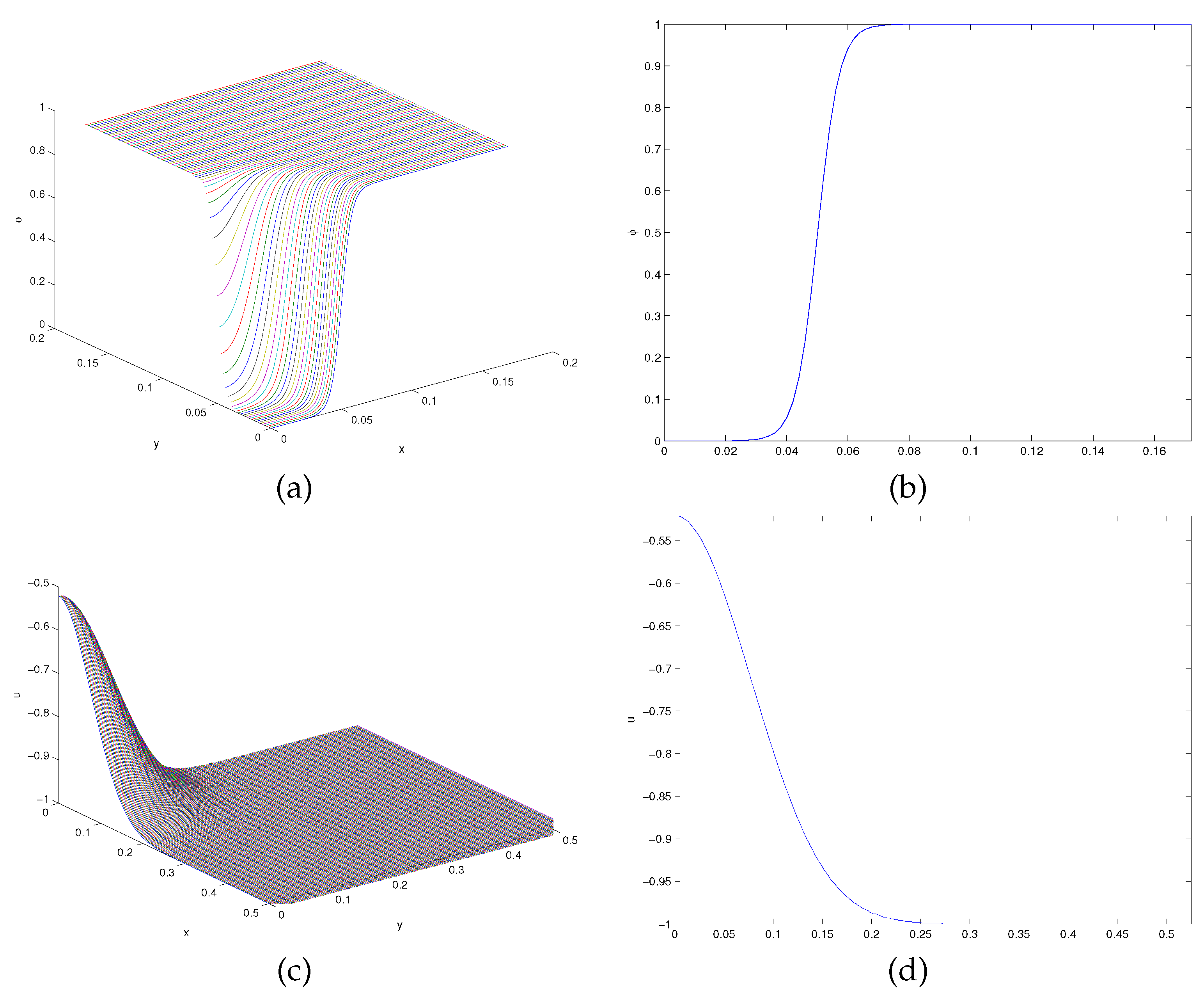
| (a) | (b) |
| (c) | (d) |
Disclaimer/Publisher’s Note: The statements, opinions and data contained in all publications are solely those of the individual author(s) and contributor(s) and not of MDPI and/or the editor(s). MDPI and/or the editor(s) disclaim responsibility for any injury to people or property resulting from any ideas, methods, instructions or products referred to in the content. |
© 2025 by the authors. Licensee MDPI, Basel, Switzerland. This article is an open access article distributed under the terms and conditions of the Creative Commons Attribution (CC BY) license (http://creativecommons.org/licenses/by/4.0/).


