A peer-reviewed article of this preprint also exists.
Submitted:
05 March 2025
Posted:
10 March 2025
You are already at the latest version
Abstract
To understand phase transition processes like solidification, phase field models are frequently employed. These models couple the energy (heat) equation for temperature with a nonlinear parabolic partial differential equation (p.d.e.) that includes a second unknown, the phase, which takes characteristic values, such as zero in the solid phase and one in the liquid phase. We consider a simplified phase field model described by a system of parabolic p.d.e’s, q(ϕ)ϕt = ∇ · (A(ϕ)∇ϕ) + f (ϕ, u), ut = Δu + [p(ϕ)]t, where ϕ(x, y, t) represents the phase indicator function and u(x, y, t) denotes the temperature. The functions q, p, and f are given scalars, and A is a 2×2 diagonal matrix dependent on ϕ. This system is posed for t ≥ 0 on a rectangle in the x, y plane with appropriate boundary and initial conditions. We solve the system using a finite difference method that uses for both equations the Crank-Nicolson-ADI scheme. We prove a convergence result for the method and show results of numerical experiments verifying its order of accuracy. The isotropic system is numerically solved using Crank-Nicolson-ADI finite difference discretization for both equations. The initial-boundary-value problem is considered with homogeneous Dirichlet boundary conditions for ϕ and u. The paper presents preliminary results on finite difference approximations, establishes the main result, showing that finite difference approximations to u and ϕ converge in the discrete L2 and H1 norms with bounds of order Δt2 + h2, given a stability condition of Δt h ≤ σ. Finally, numerical experiments confirm the convergence orders.
Phase transition processes like solidification are often understood using phase field models. These models couple the energy (heat) equation for temperature with a nonlinear parabolic partial differential equation (p.d.e.) that includes another unknown, the phase, which takes values such as zero in the solid phase and one in the liquid phase. Phase field models provide a framework for describing microstructures and capturing the dynamics of interfaces and complex patterns during solidification. The phase field distinguishes between states of matter, with the phase variable set to zero in the solid phase and one in the liquid phase. This allows the simulation of phenomena like dendritic growth and intricate patterns at the solid-liquid interface.
Phase field models [6] are versatile and can be adapted to study various physical processes beyond solidification, including melting, precipitation, and alloy formation. They incorporate various physical parameters and boundary conditions, making them suitable for theoretical and practical applications in materials science. The coupling of the heat equation with the phase field equation enables the study of thermal gradients, cooling rates, and other factors on microstructural evolution during phase transitions, providing insights into the mechanisms driving these processes and aiding in material design.
These models have been widely used to describe phase transition phenomena such as solidification. In these models, the energy equation for temperature is coupled with a nonlinear parabolic p.d.e. involving the phase, which takes values like zero in the solid and one in the liquid phase, showing a large gradient near the interface. The solution from initial conditions should show a sharp moving front representing the interface and describe complex geometric patterns (dendrites) in solidification problems. Accurate numerical solutions require fine spatial discretizations around the interface and small time steps, which are time-consuming even in two dimensions.
In this note, we consider a specific system in two dimensions, simplifying a model by McFadden, Wheeler, Sekerka, Wang et al. [13]−[16]. This “isotropic” model consists of a system of two p.d.e’s of the form
where is the phase indicator function and is the temperature, both defined on a rectangle in the plane for . The functions f and p are given smooth scalar functions of their arguments and A is a matrix given by
where are smooth function of The system (1) is supplemented by given initial conditions , , , and boundary conditions of Neumann or Dirichlet type for and u on the boundary of for . In its fully nonlinear “anisotropic” version, where A is a function of the system has been solved numerically by Wang [15], and Wang and Sekerka [16], using an ’explicit-implicit’ finite difference scheme. This scheme employs the explicit Euler method to advance the phase field over a temporal step via the first p.d.e., and then uses an ADI (Alternating Direction Implicit) scheme to solve for the temperature field in the second p.d.e. These references include numerous interesting numerical computations and measurements of the efficiency of the underlying numerical technique. In related work, Rappaz and his collaborators [2]–[4] considered similar systems and proved the existence and uniqueness of weak solutions. They also constructed and implemented fully discrete, adaptive finite element methods, using them to simulate dendritic growth in the anisotropic case. Furthermore, in [9]–[11], we constructed and implemented a Crank-Nicolson-ADI finite difference scheme for both equations in the general anisotropic case, demonstrating how it can be used in a parallel algorithm to efficiently solve the dendrite generation problem. In this note, we solve the isotropic system numerically using a finite difference discretization of the Crank-Nicolson-ADI type for both equations. We consider the initial-boundary-value problem with homogeneous Dirichlet boundary conditions for and u on the boundary of (The Neumann problem may be similarly analyzed.) In Section 2, we state the p.d.e. problem and the assumptions on its coefficients. Section 3 presents preliminary results on various finite difference approximations. In Section 4, we state and prove the main result of the paper, establishing that the finite difference approximations to u and converge in the discrete and norms, respectively, with bounds of order , where is the time step and h the uniform spatial discretization mesh length, under a stability condition of the form . We conclude by presenting simple numerical experiments that verify the orders of convergence. This comprehensive approach not only provides valuable insights into the numerical methods but also validates their efficiency and accuracy through practical implementation and testing. The results demonstrate the robustness of the Crank-Nicolson-ADI scheme in handling complex phase transition problems and pave the way for future research and applications in the field of materials science and computational physics.
2. The Problem
This “isotropic” model consists of a system (1) of two p.d.e’s is supplemented by given initial conditions , , , and boundary conditions of Neumann or Dirichlet type for and u on the boundary of for . Let For where we consider the initial-boundary-value problem
where a and are smooth functions of such that for and f and p are smooth functions defined on and respectively, with and We suppose that on Furthermore, we make the assumption (in order to simplify the proofs of the error estimates) that the functions , and p are globally Lipschitz functions of their arguments, i.e. that there exists a constant C such that:
for all We will assume that the initial-boundary-value problem (83) has a unique solution , smooth enough for the purpose of the numerical approximations.
3. Notation and Preliminary Results
We discretize the initial-boundary-value problem (83) as follows. Let where J is a positive integer and . We define and . Let N be positive integer and where and define and
We approximate the solution of (83) by mesh functions as follows: For we approximate the vectors by satisfying the following finite difference scheme:
where
We also let for (The quantities are defined analogously.) In addition, we let
Replacing the above relation in (48.(vi)) we get for
Conversely, suppose that (50) holds. Then, defining from (49) we see that (48.(vi)) and (48.(vii)) are valid. Hence the relations (48.(vi)-(vii)) are equivalent to (49)-(50). Similarly, subtracting (48.(iii)) from (48.(iv)), we see, for
and therefore
Finally, substituting in (48.(iii)) we get for
Conversely, let (52) hold. Then, if we define from (51), we see that (48.(iii)) and (48.(iv)) are equivalent to (52) and (51).
While the solution algorithm is given by the equations (48), the error analysis will be based on (50) and (52). It is clear that solving in (48) for requires the solution of symmetric tridiagonal systems of equations in each case. There systems are clearly invertible in view of our assumptions on the functions a and
In what follows we list a few auxiliary helpful results whose proofs are standard and may be found in [10].
Lemma1.
a)
Let Then
b)
Let Then
c)
If then for
i)
ii)
iii)
iv)
v)
For define the inner product on by with corresponding norm
Lemma2.
Define by
Then, there hold that
and
where is a discrete norm.
Lemma3.
Define by
Then, there holds that
and
Lemma4.
Define, for the bilinear form as
Then, for some constants independent of there holds that
where
4. Error Estimation
4.1. Local Error
We define first the local error of the scheme (48). Let be the solution of (43). For we let
and
where and Then by Taylor’s theorem we have the following local error estimate, whose proof, long but straightforward, is omitted.
Lemma5.
Suppose that the solution of (43) is sufficient smooth. Then, there exist constants independent of h such that
4.2. Error Estimate
We now prove the main result of paper.
Theorem1.
Suppose that the solution of (43) is sufficient smooth. Let be the solution of (48). Suppose that where σ is sufficiently small and that where Then, there exists a constant C independent of and h such that
Proof:
In the sequel C will denote generic constants independent of and At various points in the proof we follow some techniques of Dendy, [5], extending them from the case of a single parabolic equation considered in [5] to the case of the parabolic system considered herein.
Let From (59) and (52) we obtain, for and
For we define , where
We define similarly the discrete quantities and and we use the notation
We finally define for
The proof proceeds inductively. Our induction hypothesis is: Suppose that the following inequality holds for
Obviously, holds for
Taking the inner product of both sides of (64) with we have for
By Lemma 8, the symmetry of and our hypotheses on we have, using the equivalence of the norms and with constants independent of h and and the notation
Therefore
In addition, there holds that
To see this consider Hölder’s inequality:
and
Applying (70) for we have,
where for we define (with ).
Therefore
From (69) we have
Using (71) with we see that
Note now that the inverse inequality holds on For we have
Hence
By the above we condude that
from which (68) follows. Now, using the induction hypotheses we will show that and
are bounded for
Indeed, from we have for a small enagh (that we consider fixed from now on) that
Hence, from Gronwall’s lemma we obtain
Hence, using the stability condition we see that
Hence
and therefore
since is bounded, as it is easily seen. Similarly we see that
Now, from (72), supposing that we have, by the stability conttion that
Therefore from (68) we have, for
and a similar bound for the term Substituting (74) in (67) we have, for
Hence, from (66) and (76) we obtain, for
Therefore, using Lemma 9, we conclude for that
We now define the following quantities
From (72), since we have
Long but straightforward calculations yield now for that
and
Substituting in (76) we have
where arbitrary.
Hence, using the Cauchy-Schwarz inequality and the arithmetic geometric mean inequality we have
In addition since we have from the mean value theorem
Since for (72) gives , we have for
Then, for suitable we see that
Hence, since at we have that where
Therefore
Summing from we have
Now, from (58)and (50) we have for
We define Taking the inner product of both sides of the above relation with we have
Using the symmetry of Lemma 4 (with and Lemma 7 and summing the above relation from to we have, since
In view of (79) we have
Hence, by Gronwall lemma we infer that
Therefore, by (60) and (61)
Hence, using we have
Since
substituting (82) and (61) in (79) we have
Take now so that so (83) gives
which is for m instead of Hence, the inductive step is complete and holds for We conclude from (81) that (62) holds.
Finally, it follows from that
from which, by Gronwall’s lemma it follows that
which implies (63).
▪
We may easily obtain from Taylor’s theorem an approximation at the first step satisfying
5. Numerical Verification of the Order of Convergence
In the sequel, we solved the system (43) under Neumann boundary conditions on (We obtained similar rates for the problems with Dirichlet boundary conditions.) We took We added a suitable nonhomogeneous term so that the solution of the associated initial-boundary-value problem with Neumann boundary conditions on was
Table 1.
Errors and order of convergence of the ADI-ADI scheme, T=0.1.
Table 1.
Errors and order of convergence of the ADI-ADI scheme, T=0.1.
J
errors
order
errors
order
50
75
112
168
252
378
567
Table 2 shows the errors and the experimental orders of convergence of the numerical solution computed by the ADI-ADI scheme for the this problem, in the discrete maximum norm and also in the norm We computed with where and The observed order of convergence is approximately equal to 2 for both variables in both norms. (For two consecutive runs with values of giving errors respectively, the rate of convergence was computed as )
With this scheme we performed two numerical experiments where we took (cf. Wang[15]) on , ,
, , where , S=dimensionless supercooling of the melt, m=ratio of the capillary to the kinetic length and ratio of the average interface thickness parameter.
In the isotropic case, with values of physical parameters given by and the evolution of the solution is’ given in Figures 1, (we took , ).
6. The Problem
This “isotropic” model consists of a system (1) of two p.d.e’s is supplemented by given initial conditions , , , and boundary conditions of Neumann or Dirichlet type for and u on the boundary of for . Let For where we consider the initial-boundary-value problem
where a and are smooth functions of such that for and f and p are smooth functions defined on and respectively, with and We suppose that on Furthermore, we make the assumption (in order to simplify the proofs of the error estimates) that the functions , and p are globally Lipschitz functions of their arguments, i.e. that there exists a constant C such that:
for all We will assume that the initial-boundary-value problem (43) has a unique solution , smooth enough for the purpose of the numerical approximations.
7. Notation and Preliminary Results
We discretize the initial-boundary-value problem (43) as follows. Let where J is a positive integer and . We define and . Let N be positive integer and where and define and
We approximate the solution of (43) by mesh functions as follows: For we approximate the vectors by satisfying the following finite difference scheme:
where
We also let for (The quantities are defined analogously.) In addition, we let
where
and
Subtracting (48.(vi)) from (48.(vii)) we have for
Solving for we get
Replacing the above relation in (48.(vi)) we get for
Conversely, suppose that (50) holds. Then, defining from (49) we see that (48.(vi)) and (48.(vii)) are valid. Hence the relations (48.(vi)-(vii)) are equivalent to (49)-(50). Similarly, subtracting (48.(iii)) from (48.(iv)), we see, for
and therefore
Finally, substituting in (48.(iii)) we get for
Conversely, let (52) hold. Then, if we define from (51), we see that (48.(iii)) and (48.(iv)) are equivalent to (52) and (51).
While the solution algorithm is given by the equations (48), the error analysis will be based on (50) and (52). It is clear that solving in (48) for requires the solution of symmetric tridiagonal systems of equations in each case. There systems are clearly invertible in view of our assumptions on the functions a and
In what follows we list a few auxiliary helpful results whose proofs are standard and may be found in [10].
Lemma6.
a)
Let Then
b)
Let Then
c)
If then for
i)
ii)
iii)
iv)
v)
For define the inner product on by with corresponding norm
Lemma7.
Define by
Then, there hold that
and
where is a discrete norm.
Lemma8.
Define by
Then, there holds that
and
Lemma9.
Define, for the bilinear form as
Then, for some constants independent of there holds that
where
8. Error Estimation
8.1. Local Error
We define first the local error of the scheme (48). Let be the solution of (43). For we let
and
where and Then by Taylor’s theorem we have the following local error estimate, whose proof, long but straightforward, is omitted.
Lemma10.
Suppose that the solution of (43) is sufficient smooth. Then, there exist constants independent of h such that
8.2. Error Estimate
We now prove the main result of paper.
Theorem2.
Suppose that the solution of (43) is sufficient smooth. Let be the solution of (48). Suppose that where σ is sufficiently small and that where Then, there exists a constant C independent of and h such that
Proof:
In the sequel C will denote generic constants independent of and At various points in the proof we follow some techniques of Dendy, [5], extending them from the case of a single parabolic equation considered in [5] to the case of the parabolic system considered herein.
Let From (59) and (52) we obtain, for and
For we define , where
We define similarly the discrete quantities and and we use the notation
We finally define for
The proof proceeds inductively. Our induction hypothesis is: Suppose that the following inequality holds for
Obviously, holds for
Taking the inner product of both sides of (64) with we have for
By Lemma 8, the symmetry of and our hypotheses on we have, using the equivalence of the norms and with constants independent of h and and the notation
Therefore
In addition, there holds that
To see this consider Hölder’s inequality:
and
Applying (70) for we have,
where for we define (with ).
Therefore
From (69) we have
Using (71) with we see that
Note now that the inverse inequality holds on For we have
Hence
By the above we condude that
from which (68) follows. Now, using the induction hypotheses we will show that and
are bounded for
Indeed, from we have for a small enagh (that we consider fixed from now on) that
Hence, from Gronwall’s lemma we obtain
Hence, using the stability condition we see that
Hence
and therefore
since is bounded, as it is easily seen. Similarly we see that
Now, from (72), supposing that we have, by the stability conttion that
Therefore from (68) we have, for
and a similar bound for the term Substituting (74) in (67) we have, for
Hence, from (66) and (76) we obtain, for
Therefore, using Lemma 9, we conclude for that
We now define the following quantities
From (72), since we have
Long but straightforward calculations yield now for that
and
Substituting in (76) we have
where arbitrary.
Hence, using the Cauchy-Schwarz inequality and the arithmetic geometric mean inequality we have
In addition since we have from the mean value theorem
Since for (72) gives , we have for
Then, for suitable we see that
Hence, since at we have that where
Therefore
Summing from we have
Now, from (58)and (50) we have for
We define Taking the inner product of both sides of the above relation with we have
Using the symmetry of Lemma 9 (with and Lemma 7 and summing the above relation from to we have, since
In view of (79) we have
Hence, by Gronwall lemma we infer that
Therefore, by (60) and (61)
Hence, using we have
Since
substituting (82) and (61) in (79) we have
Take now so that so (83) gives
which is for m instead of Hence, the inductive step is complete and holds for We conclude from (81) that (62) holds.
Finally, it follows from that
from which, by Gronwall’s lemma it follows that
which implies (63).
▪
We may easily obtain from Taylor’s theorem an approximation at the first step satisfying
9. Numerical Verification of the Order of Convergence
In the sequel, we solved the system (43) under Neumann boundary conditions on (We obtained similar rates for the problems with Dirichlet boundary conditions.) We took We added a suitable nonhomogeneous term so that the solution of the associated initial-boundary-value problem with Neumann boundary conditions on was
Table 2.
Errors and order of convergence of the ADI-ADI scheme, T=0.1.
Table 2.
Errors and order of convergence of the ADI-ADI scheme, T=0.1.
J
errors
order
errors
order
50
75
112
168
252
378
567
Table 2 shows the errors and the experimental orders of convergence of the numerical solution computed by the ADI-ADI scheme for the this problem, in the discrete maximum norm and also in the norm We computed with where and The observed order of convergence is approximately equal to 2 for both variables in both norms. (For two consecutive runs with values of giving errors respectively, the rate of convergence was computed as )
With this scheme we performed two numerical experiments where we took (cf. Wang[15]) on , ,
, , where , S=dimensionless supercooling of the melt, m=ratio of the capillary to the kinetic length and ratio of the average interface thickness parameter.
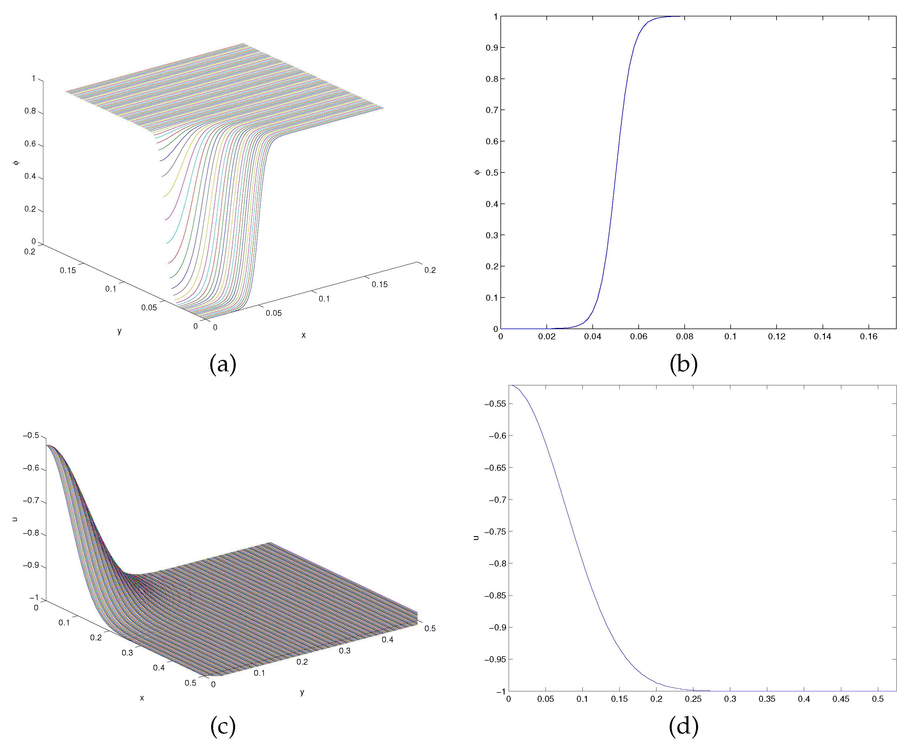
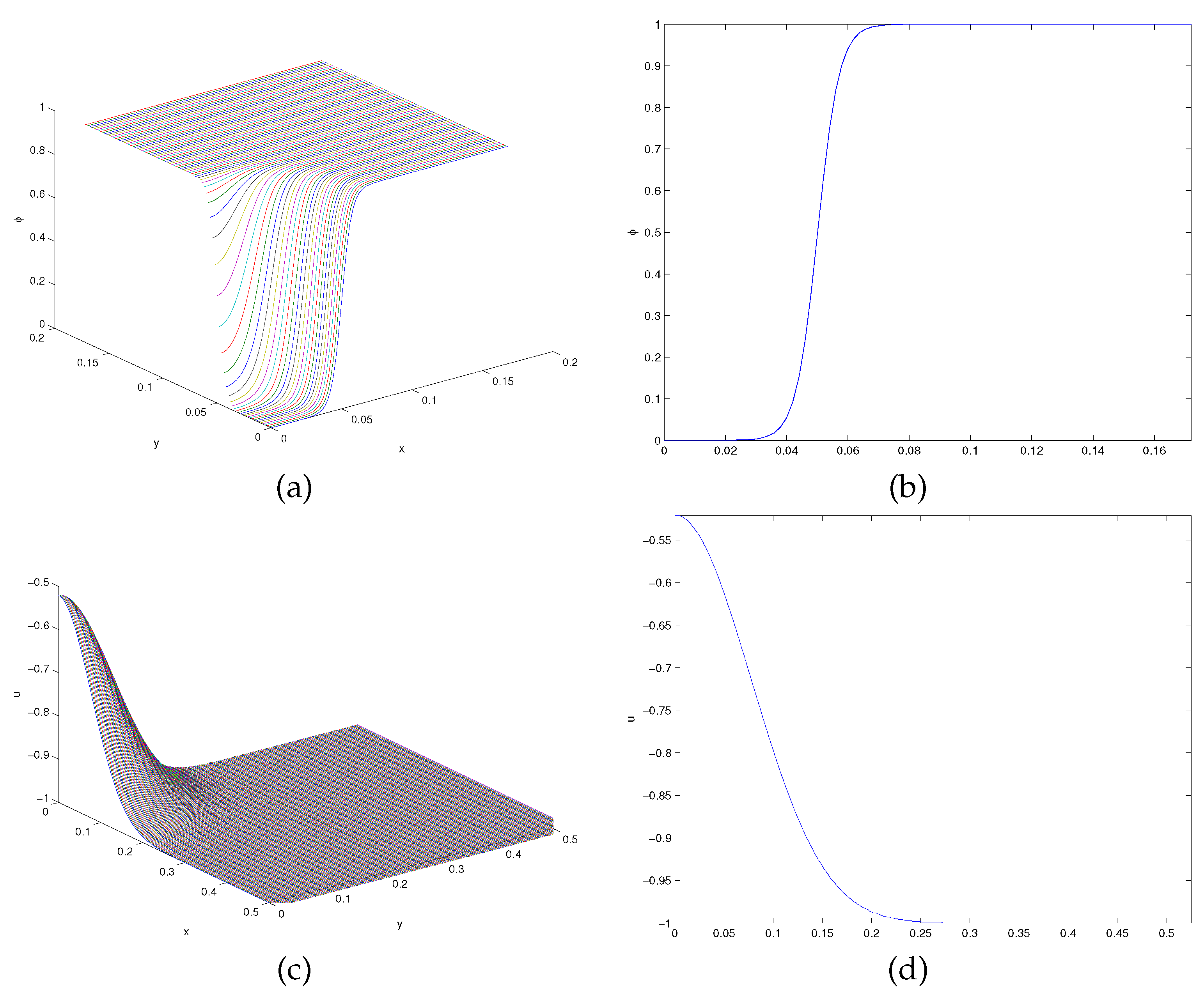
In the isotropic case, with values of physical parameters given by and the evolution of the solution is’ given in Figures 1, (we took , ).
Figure 3.
the isotropic case. (a):3D plot of (b):trace at of (c):3D plot of (d): trace at of u (all at ).
Figure 3.
the isotropic case. (a):3D plot of (b):trace at of (c):3D plot of (d): trace at of u (all at ).
(a)
(b)
(c)
(d)
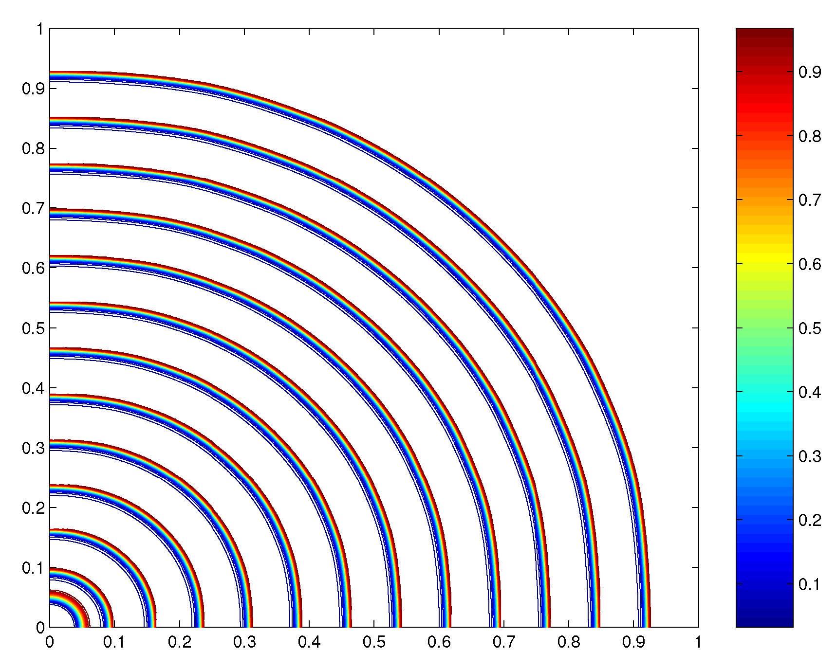
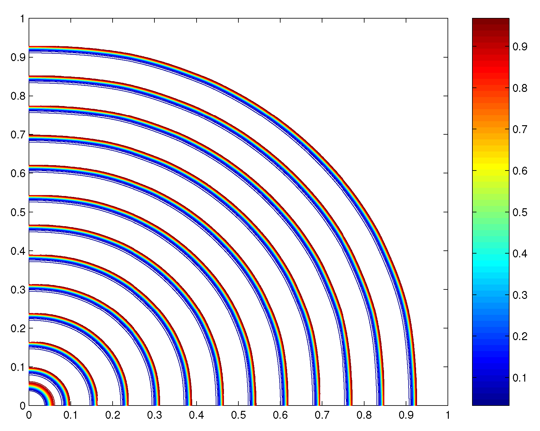
Figure 4.
Succesive contours of the interface of every 100 time steps for the isotropic case.
Figure 4.
Succesive contours of the interface of every 100 time steps for the isotropic case.
Acknowledgments
We express our gratitude to the reviewers for their insightful remarks and suggestions, which greatly enhanced the quality of the current paper. However, I would like to express my gratitude to Professor V. Dougalis for their invaluable guidance and revisions in this research. The author acknowledge financial support for the dissemination of this work from the Special Account for Research of ASPETE through the funding program “Strengthening research of ASPETE faculty members”.
References
B. Billia and R. Trevedi, “Pattern formation in crystal growth”, in M. E. Glicksman and S. P. Marsh, “The dendrite”, in Handbook of Crystal Growth, Vol. 1, ed. by D.T.J. Hurle, North-Holland, Amsterdam, 1993.
E. Burman and J. Rappaz, “Existence of solutions to an anisotropic phase field model”, Mathematical Methods in the Applied Sciences, Vol. 26 (2003), pg. 1137-1160. [CrossRef]
E. Burman, M. Picasso. and J. Rappaz, “Analysis and computation of dendritic growth in binary alloys using a phase-field model”, to appear in Proccedings of ENUMATH conference.
E. Burman, D. Kessler, J.Rappaz, “Convergence of the finite element method applied to an anisotropic phase-field model”, Annales Math. B. Pascal, Vol. 11 (2004), pg. 69-95.
J.E. Dendy, “Alternating direction methods for nonlinear time-depedent problems”, SIAM .I. Numer. Anal., Vol. 14 (1977), pg. 313-326.
J.S. Langer, “Models of pattern formation in first-order phase transitions”, in Directions in Condensed Matter Physics, ed. By G. Grinsteil and G. Mazenko, World Scientific, Singapore 1986, pg. 164-186.
N. Provatas, N. Goldenfeld, and J.A. Dantzig, "Efficient computation of dendritic microstructures using adaptive mesh refinement", Physical Review Letters, Vol. 80 (1998), pp. 3308-3311. [CrossRef]
Chr. A. Sfyrakis and V. A. Dougalis, “A fast numerical method for a simplified phase field model”, in Mathematical Methods in Scattering Theory and Biomedical Engineering, ed. by World Sci. Publ., Hackensack, NJ, 2006, pg.208–215.
Chr. A. Sfyrakis, “Mathematical and numerical models for materials phase change problems”, Ph.D. thesis, Department of Mathematics, University of Athens, (in Greek,) 2008.
Chr. A. Sfyrakis, “A numerical method for a simplified anisotropic phase field model”, in Bull. Greek Math. Soc. Vol. 54, (2007), pg. 273–279.
Chr. A. Sfyrakis, “Finite difference methods for an anisotropic phase field model”,Recent Advances in Mathematics and Computers in Biology and Chemistry, ed. by WSEAS Press, 2009, pg. 142-146.
Chr. A. Sfyrakis, G. E. Chatzarakis, Sp. L. Panetsos, “Estimate of an Error for a Finite Difference a Phase Field Model for the Euler-Crank-Nicolson Methods”, Journal of Applied Mathematics and Computation, 2022, Volume 6(4), 431-449, ISSN Online: 2576-0653, ISSN Print: 2576-0645. [CrossRef]
C.B. McFadden, A.A. Wheeler, R.J. Braun, S.R. Coriell and R.F. Sekerka, “Phase-field models for anisotropic interfaces”, Physical Review E, Vol. 48, (1993), pg. 2016-2024. [CrossRef]
S. L.Wang, “Computation of dendritic growth at large supercoolings by using the phase field model”, Ph.D. thesis, Department of Physics, Carnegie-Mellon University, Pittsburgh, 1995.
S. L. Wang and R. F. Sekerka, “Algorithms for phase field computation of the dendritic operating state at large supercoolings”, Journal of Computational Physics, Vol. 127 (1996), pg. 110-117. [CrossRef]
Figure 1.
the isotropic case. (a):3D plot of (b):trace at of (c):3D plot of (d): trace at of u (all at ).
Figure 1.
the isotropic case. (a):3D plot of (b):trace at of (c):3D plot of (d): trace at of u (all at ).
(a)
(b)
(c)
(d)
Figure 2.
Succesive contours of the interface of every 100 time steps for the isotropic case.
Figure 2.
Succesive contours of the interface of every 100 time steps for the isotropic case.
Disclaimer/Publisher’s Note: The statements, opinions and data contained in all publications are solely those of the individual author(s) and contributor(s) and not of MDPI and/or the editor(s). MDPI and/or the editor(s) disclaim responsibility for any injury to people or property resulting from any ideas, methods, instructions or products referred to in the content.
Copyright: This open access article is published under a Creative Commons CC BY 4.0 license, which permit the free download, distribution, and reuse, provided that the author and preprint are cited in any reuse.
Preprints.org is a free preprint server supported by MDPI in Basel, Switzerland.