
Submitted:
05 March 2025
Posted:
06 March 2025
You are already at the latest version
Abstract
PDE-based hydrologic models demand extensive preprocessing, which can create a bottleneck and slow down the model setup process. Mesh generation typically lacks integration with hydrological features like river networks. To address this, we present GHOST Mesh (GMesh), an automated, watershed-oriented mesh generator built within the Watershed Modeling Framework (WMF). While primarily designed for the GHOST hydrological model, GMesh’s functionalities can be adapted for other models. GMesh enables rapid mesh generation in Python by incorporating Digital Elevation Models (DEM), flow direction maps, network topology, and online services. The software creates Voronoi polygons that maintain connectivity between river segments and surrounding hillslopes, ensuring accurate surface-subsurface interaction representation. Key features include customizable mesh generation and variable refinement to target specific watershed areas. We applied GMesh to Iowa’s Bear Creek watershed, generating meshes from 10,000 to 30,000 elements and analyzing their effects on simulated stream flows. Results show higher mesh resolutions enhance peak flow predictions and reduce response time discrepancies, while local refinements improve model performance with minimal additional computation. GMesh’s open-source nature streamlines mesh generation, offering researchers an efficient solution for hydrological analysis and model configuration testing.
Keywords:
Mesh generation
; PDE-based hydrological models
; flooding
1. Introduction
[1] introduced the blueprint for physically based digitally simulated watershed models. Later, [2] described their main features, highlighting their focus on surface-subsurface interactions relying on differential equations solved over a computational mesh. In addition to the significant data for parameterization, the mesh generation process is time-consuming and tedious when not fully automated. These factors partly explain why physically-based watershed modeling has not become widely used in hydrology despite some improvements in recent years [3]. Manual mesh generation can often take significant time, ranging from days to weeks, depending on the complexity of the watershed and the spatial resolution required, creating a major bottleneck in modeling workflows. Similar challenges have been documented in hydrological modeling and other computational domains [4,5]. Challenges with mesh generation processes are not unique to hydrology; other disciplines that rely on mesh-based simulations have identified similar problems. For example, a report by NASA on computational aero science states that "mesh generation and adaptivity continue to be significant bottlenecks in the Computational Fluid Dynamics workflow [6]." In hydrological modeling, the accuracy and computing time heavily depend on the mesh and the network used to represent the watershed [7,8]. However, there is still a bottleneck around mesh generation that considers the connectivity between the network and hillslope elements [9].
Several mesh generation tools have been developed for hydrologic modeling. Some examples include the Triangle Software [10], HydroGeoSphere [11], Hydrus3D [12], and Gmsh [13]. Nevertheless, most of these tools require intensive manual intervention or editing of several configuration files. In the case of Hydrus3D and Delft3D [14], most of the work uses graphical user interfaces (GUIs), which facilitate the work but, at the time, impose configuration and automation limitations along with paywalls.
We developed GMesh to fill this gap, allowing modelers to quickly set up a mesh for a watershed using the Digital Elevation Model as a starting point. The need for an automated, flexible mesh generator capable of handling watershed-scale simulations has become increasingly evident as the complexity and scope of hydrological projects continue to grow [15,16]. We developed GMesh, a mesh generator designed for hydrological modeling to address those challenges. We built GMesh on top of the Watershed Modeling Framework (WMF)[17], a Python interface that allows hydrologic analysis and simulation using code. This feature allows users to automate the mesh generation process while exploring multiple configurations. Along with WMF, GMesh allows generation meshes with different configurations, the specification of refinement areas, and changes in the network threshold definition, and automatically assigns properties to the generated polygons. This paper presents the development of GMesh and its implementation within the GHOST hydrological model.
2. Materials and Methods
The GHOST mesh generator (GMesh) has been developed as a class of the Watershed Modeling Framework (WMF) [17]. WMF is a Fortran-Python module designed to provide tools to perform hydrological analysis and modeling that conceptualizes the watershed as an object with a defined topology, properties, and functions. As shown in [17], with WMF, a Python user can quickly delineate a watershed and extract several characteristics of it, including the required files to run the TETIS model [18,19] and the Hillslope Link Model (HLM) [20]. GMesh constitutes an additional set of tools that allows us to set up the mesh and files required by GHOST [2]. In the following sections, we describe GMesh architecture and usage.
2.1. GMesh Architecture
We developed GMesh on top of the watershed cell structure defined by WMF. Its execution requires a Digital Elevation Model (DEM) and a single direction map (D8) [21]. Also, the watershed structure must have a defined accumulated area threshold that defines the startup point of the cells with channels. From this point, GMesh generates the channel network segments' topology and the corresponding mesh points, computes the Voronoi polygons, and defines the topological connection between them. Figure 1 presents a summary of the described steps, and we explain each step in detail.
2.1.1. Network Pre-Processing
The network is the primary driver of GMesh. As a first step, GMesh obtains a version of the network in which each channel reach is reduced into a set of segments with the same or less complex geometry. Then, GMesh defines the segment's connectivity from upstream to downstream using the network connectivity defined by WMF. GMesh also checks for elevation coherence between upstream and downstream segments in this process. GMesh adjusts river segment elevations, ensuring that the downstream elevation of each segment is lower than the upstream elevation. We show the described process in Figure 1b.
2.1.2. Mesh Generation
Once GMesh obtains the network segments, it defines the coordinates of the points that will generate the mesh using the river segments and the user-defined grid size. The first coordinates of the mesh correspond to points surrounding the network segments. At every segment, GMesh defines coordinates over lines perpendicular to the segment. The distance between perpendicular lines and the length of each line defines the density of points surrounding the network. The user can adjust both parameters. Then, GMesh removes overlapping or too-close points using a threshold minimum distance. At the end of this process, GMesh obtains a collection of points surrounding the segments (Figure 1c). Once the segment points are defined, GMesh proceeds to populate the points collection with a regular grid of pre-defined distance and removes the ones close to the segment points (green points in Figure 1d). Finally, GMesh uses a dilation process on the WMF watershed definition to obtain the borderline points (orange points in Figure 1d). The border defines the coordinates that define the end of the watershed.
2.1.3. Polygons Definition
With the mesh points defined, GMesh computes the Voronoi polygons and extracts their connectivity. This procedure starts by extracting the Voronoi polygons, differentiating between valid points (river network and regular grid) and invalid ones (border points). Then, GMesh eliminates the polygons that belong to the invalid class or have no valid neighbors (Figure 1e). This process also determines the neighbor of each polygon. After the nestwork and mesh generation process is complete, GMesh determines each river segment's left and right polygons. These polygons will be connected with the river segment during the GHOST execution. Finally, GMesh checks for elevation correctness and reduces the number of faces of the polygons that are over the watershed boundary.
Once the segment network and the polygons are defined, GMesh can write the input files required by GHOST. The input files include a mesh file indicating the polygon faces, their connectivity, and properties, a river file with the segment's topology and properties, and the vectorial files corresponding to both. Also, GMesh offers the option to retrieve the polygon's soil and land use properties using the Google Earth Explorer (GEE) API for Python. For this option, the user must set up a GEE account.
2.1.4. Localized Mesh Refinement
In addition to the previously described process, GMesh allows mesh refinement to be specified in areas of interest. Moreover, this refinement can have distinct parameters between areas. When active, the refinement option prompts for the distance between the points of the grid mesh, the distance between perpendicular lines along the river segments, and the length of these lines. We included this option to increase the simulation detail level at specific regions in GHOST. Refinement is highly useful for inquiring about specific processes and improving the model performance [22,23]. In the results section, we present an example of a mesh generated using the local refinement option.
2.2. Functions and Usage
The previously described steps can be found in the ghost_preprocess class. As mentioned before, the class uses the WMF watershed class as a primary input, as well as the path to the DEM, the specified length of the network segments, and, optionally, the refinement parameters. After its definition, the user can iterate over the following class functions:
- Get_segments_topology: Obtains the connectivity between the new channel segments (Figure 1b).
- Get_mesh_river_points: Obtains the coordinates of the points surrounding each network segment. It extracts two points per segment, one over the left and the other over the right (Figure 1c).
- Get_mesh_grid_points: Defines the coordinates of a regular grid used to populate the mesh inside the watershed (Figure 1d).
- Get_vornoi_polygons: Derives the polygons using the river, regular grid, and border mesh points. Also, it differentiates between them.
- Define_polygons_topology: Defines the valid polygons, the connectivity between them, their connectivity with the segments network, and their properties (Figure 1e).
The described functions can be used in series or independently, allowing easy changing of the segments and polygon configuration for a given watershed. The refinement option can be activated when setting up the project in ghost_preprocess using a dictionary that indicates the key that identifies a refinement area and its parameters.
3. Results
Using the WMF preprocessor along with GMesh, we set up finite element discretization for the Bear Creek watershed, Iowa (with an area of around 200 ). Using GHOST, we tested the mesh generated using different options and configurations. The examples include a basic mesh development, the use of focus regions, and testing the effect of the mesh resolution on GHOST. We describe the steps and results obtained in each and examples of the simulations obtained by GHOST using the provided setups.
3.1. Bear Creek Watershed Example
This example presents a mesh generated for the Bear Creek watershed (Figure 2) using a DEM of 30m and its corresponding D8 map (Figure 3a and b, respectively). Bear Creek is a tributary of the Upper Iowa River. The watershed encompasses a landscape characterized by steep terrain that is prone to erosion. This susceptibility has led to concerns over excessive soil erosion affecting the basin's croplands, pastures, and forests. The Bear Creek Watershed Project has implemented efforts to mitigate these issues, aiming to enhance water quality by reducing pollutants such as ammoniated manure. Additionally, the creek frequently experiences flooding, exacerbating erosion and sediment transport, posing challenges for water management in the region.
According to the DEM, the watershed exhibits an elevation gradient of around 200m with steeper slopes in northern regions close to the watershed boundary. Moreover, the D8 map shows a well-defined network. The Bear Creek watershed in northeastern Iowa features rolling hills and steep slopes within the Driftless Area, a rugged region unaffected by glaciation. Its geology includes limestone and dolomite, creating karst features like sinkholes and springs influencing water flow. Soils derived from loess and alluvium vary from well-drained upland soils to poorly drained lowland soils.
As described in [24], we used the flow direction raster (Figure 3b) to obtain the Voronoi polygons, generating a detailed representation of the watershed's hydrological features. The raster, classified into nine distinct categories, illustrates the various water flow directions within the study area. The DEM (Figure 3a) highlights the topographical variation within the watershed, with elevation values ranging from 245.76 meters to 407.22 meters. The model provides a comprehensive overview of the terrain, showcasing high elevation in white and lower elevation in green. This elevation data is essential for understanding the watershed's slope and gradient, directly impacting water flow and erosion processes.
3.2. Mesh Stability Evaluation
We evaluated the mesh stability in GHOST using three different refinement levels with ten thousand, fifteen thousand, and thirty thousand elements (see Figure 4). We controlled the mesh quality by limiting the polygon's maximum number of faces to 19 and by using a flow accumulation threshold of 300. The results in Table 1 show that the average number of faces is inversely proportional to the number of elements. With many elements, the average number of faces decreases, resulting in more stable meshes. Conversely, fewer elements increase the average number of faces, leading to more unstructured meshes and unstable GHOST executions. Additionally, we evaluated how the total number of elements changed the computational time required to generate the mesh (see Table 1).
According to our results, the computational time to generate the mesh increases proportionally with the number of elements. However, this increase is not linear. For 10,000 elements, the generation time is 10 minutes, with an average of 11 faces per element. For 15,000 elements, the generation time increases to 20 minutes, with an average of 8 faces per element. For 30,000 elements, the generation time increases to 35 minutes, with an average of 7 faces per element.
The increase in generation time with the number of elements is expected due to the higher computational load required to process larger datasets. However, the decrease in the average number of faces per element with increasing elements suggests a more efficient mesh generation at higher resolutions. This efficiency is crucial for detailed hydrological modeling, allowing for more precise simulations without excessively prolonging computation times.
We ran GHOST using the three meshes, obtaining different results at the outlet (Figure 5). According to the results, there is a difference in the peak magnitude and the time to peak between the meshes. The high-resolution mesh (with ~ 30K elements) exhibits a higher peak flow and a faster response, while the lower resolution (~ 10K elements) has a lower peak and a slower response. Various authors have reported similar results before. Using the CASC2D-Sed model, [8] showed how coarser DEM resolutions reduced total runoff and peak flow. Moreover, using a finite element hydraulic model [25] shows how the resolution of an irregular triangular mesh reduces the model performance. There is little information on this matter for models like GHOST (physically based and irregular mesh-based). However, our results indicate that mesh resolution also plays a significant role in inducing significant changes in the simulations.
Higher mesh resolution increases the simulated peak and the response time of the GHOST model. Also, it induced slight changes in the shape of the hydrograph, altering the recession curve and the rising limb. Nevertheless, a higher resolution on the mesh also increased the model execution times (see Table 2). Here, we explored the mesh resolution effects for a watershed of around 200. However, for larger watersheds, the execution times may increase dramatically, making the high-resolution representation impractical. On the other hand, the resolution effect may change with the watershed scale. We anticipate higher effects over small scales, making the correct selection of the mesh resolution more relevant for these cases. The selection of a proper discretization is of high relevance and can determine the model performance and its parameterization [26,27,28]. Further studies of this issue using GMesh and GHOST would include the analysis at more scales and under different environments. However, it is out of the scope of this work.
3.3. Local Mesh Refinement
To overcome the execution time limitation for large watersheds while representing processes at a relatively high resolution, we included the local mesh refinement option in GMesh. The local refinement of the mesh is activated by activating the focus_map and focus_dict options when calling the ghost_preprocess function. The focus_map points to a raster map with categories (numbers) indicating regions with different levels of refinement (e.g., 1, 2, 3, etc.). The focus_dict is a Python dictionary where each category has a sub-dictionary with the parameters to build the mesh (segment threshold, mesh distance, segment-to-point distance, etc.). In Figure 6, we present an example of this map indicating three different categories: 1 for the focused areas, 3 for the areas around the channels network, and 2 for the remaining areas.
The focus function effectively enhances the mesh resolution in areas of interest, providing a more detailed representation of the watershed. This refinement is crucial for capturing the small-scale hydrological processes that significantly impact the overall simulation accuracy. Also between the 10K meses with and without focus areas, the GHOST computational remains similar (Table 3 and Table 4).
Additionally, the mesh generation cost increased by only two minutes, which is a reasonable trade-off given the reduction in hydrological computational time.
The hydrograph in Figure 7 illustrates the outflow over time for different mesh configurations, comparing the standard ten thousand (10k) mesh with the ten thousand (10k – focus_mesh) refined areas mesh. The results demonstrate that the locally refined mesh provides a more accurate depiction of the peak flow and recession limb, highlighting the benefits of using the focus function for hydrological simulations. The locally refined mesh captured the hydrological behavior more precisely, particularly in critical areas of the watershed, leading to better predictions of peak flow and recession patterns. Additionally, regardless of the resolution increase, the computational efficiency remained manageable, demonstrating the practicality of using the focus function for large-scale hydrological modeling.
4. Discussion
The development of GMesh tackles the hydrological modeling challenge of generating computational meshes that accurately capture hydrological features while remaining computationally efficient. Traditional mesh generation approaches often require substantial manual work, are disconnected from watershed hydrological characteristics, and are time-consuming [6]. We designed GMesh to address these issues by automating the process and enabling the direct use of Digital Elevation Models (DEM), flow direction maps, and river network topology. This integration, frequently overlooked in existing tools [11,13], streamlines mesh generation and ensures hydrologically consistent meshes.
We present different GMesh examples using the Bear Creek watershed highlighting its capacity to generate meshes that improve the performance of the GHOST model. Simulations using higher-resolution meshes showed differences in the peak flow predictions and faster response times. Our results align with previous studies noting the sensitivity of hydrological models to mesh resolution [8,25]. The differences stem from a more detailed representation of surface-subsurface interactions and terrain features. Additionally, the local mesh refinement allowed us to focus computational resources on key areas of the watershed, yielding detailed simulations without significantly increasing overall computation time. This feature offers a practical advantage over traditional uniform refinement methods [22,23]. Moreover, it bridges the gap between computational modeling and real-world hydrological processes. Variable refinement enables targeted simulations, which is particularly beneficial when working with large watersheds or under computational constraints. This approach aligns with the need for balanced model complexity and efficiency, as emphasized by [15].
Despite these advancements, certain limitations warrant further exploration. While mesh generation time grows with the number of elements, it does not scale linearly, leaving room for optimization. Additionally, the accuracy of generated meshes is highly dependent on input data quality, especially the DEM and flow direction maps. Although GMesh was developed with the GHOST model in mind, extending its compatibility with other hydrological models would broaden its applicability.
Although the change in the resolution and the local refinement presented distinct outflows, we have no information regarding their change in the performance. We require additional experiments to test the effects of the discretization scale on the model performance. Here, we present results at the outlet of the watershed without performing comparisons with observations or at nested sub-watersheds. Previous experiments highlight how network aggregation can blur model assessment downstream [29]. Extending these results to our case, it is hard to determine the impact of the mesh resolution at smaller channel reaches. Nevertheless, the software presented here allows for performing systematic evaluations. Moreover, it also allows robust assessments of the mesh refinement effects.
The comparison of different mesh resolutions underscored the importance of balancing accuracy and computational efficiency. We suspect that higher resolution meshes provided more accurate predictions of hydrological behaviors, while the ability to refine specific areas within the watershed allowed for targeted simulations of critical processes. Nevertheless, our goal is to illustrate the versatility of GMesh when implementing and testing different hydrological model configurations. Moreover, its integration with Google Earth Explorer (GEE) API further enhances its flexibility, making it a comprehensive tool for watershed hydrology.
Future research should focus on evaluating GMesh across diverse watershed scales and environments to assess its generalizability. Incorporating real-time data streams and developing adaptive refinement strategies responsive to dynamic hydrological conditions could further enhance forecasting applications. There is also potential to improve computational performance through parallelization or leveraging GPU processing, particularly for large-scale simulations.
5. Conclusions
This study introduced GMesh, an automated watershed-oriented mesh generator integrated with the Watershed Modeling Framework (WMF) for use in physically-based hydrological models. GMesh streamlines the traditionally labor-intensive process of mesh generation, allowing for the efficient creation of computational meshes with varying levels of detail. We present different examples where we ran the GHOST model using meshes generated by GMesh, demonstrating its ability to obtain stable and structured meshes. The flexibility offered by GMesh, particularly its ability to perform local refinement, makes it a powerful tool for hydrological simulations requiring detailed and iterative processes.
GMesh achieves this by integrating digital elevation data (DEM) and flow direction maps to delineate the watershed structure and identify the channel network. The software then generates mesh points around these network elements using Voronoi polygons, ensuring that the spatial relationships between land and river segments are preserved. This process creates a mesh where each polygon is oriented toward hydrological processes, with the ability to capture both the terrain's topographical characteristics and the flow dynamics of the watershed. By automating the recognition and connectivity of land and network elements, GMesh produces meshes that are inherently suited for physically-based hydrological simulations, ensuring accuracy in surface-subsurface interaction modeling.
We validated GMesh by applying it to the Bear Creek watershed, Iowa (200 ). The validation consisted of a series of experiments showing the GMesh capabilities and how it can benefit the implementation of finite element-based hydrological models. First, we presented a straightforward implementation using the same level of refinement. Then, we evaluated GMesh stability by generating meshes of different refinement levels for Bear Creek. Finally, we presented an example of how the local refinement works. For the refinement levels, we created three meshes with a total number of elements varying between 10 and 30K. In this case, we presented the changes in the mesh generation time and the average number of faces of the generated polygons. Also, we contrasted the differences between GHOST simulations, obtaining a higher peak flow for the refinement of 30K. Moreover, we also illustrate differences between simulations with and without local mesh refinement (section 3.3).
However, despite these strengths, GMesh has several limitations that warrant further development. The computational time required for generating high-resolution meshes increases significantly. Additionally, the accuracy of the mesh is highly dependent on the quality of input data, such as the DEM, and uncertainties in the flow direction maps. While GMesh allows for local refinement, further optimization is needed to improve its performance in regions with complex topography. Finally, the current version of GMesh is primarily compatible with the GHOST model, which restricts its use for users working with other hydrological models. Therefore, future work may explore expanding compatibility and optimizing its compatibility with other models.
In summary, GMesh provides a practical solution for hydrologists seeking to generate high-quality meshes efficiently. Automating a traditionally labor-intensive process and preserving key hydrological connections enables more accurate, flexible, and computationally manageable simulations. This tool serves both researchers and practitioners aiming to improve hydrological analysis and decision-making processes.
Supplementary Materials
The pre-processing code is included as a branch of the Watershed Modelling Framework (WMF) in GitHub and can be found at: https://github.com/nicolas998/WMF/tree/ghos_topo. This is a free and open software available since 2021 written in Fortran and Python. It requires a Python 3.X interpreter and a Fortran compiler (we tested it using gFortran). For a complete description of each function and examples of their usage, please refer to: https://github.com/nicolas998/WMF/blob/develop/Examples/BearCreek_Watershed_Oriented_Mesh_Generator.ipynb.
Author Contributions
Conceptualization, N.V. and A.A.; methodology, N.V.; software, N.V. and M.D; validation, M.D.; formal analysis, M.D and N.V.; investigation, N.V., A.A., and M.D.; resources, N.V and A.A.; data curation, M.D.; writing—original draft preparation, N.V.; writing—review and editing, M.D and A.A.; visualization, M.D and N.V.; supervision, N.V and A.A.; project administration, N.V. and A.A.; funding acquisition, N.V, and A.A. All authors have read and agreed to the published version of the manuscript.
Funding
This research was partially funded by the Mid-America Transportation Center via a grant from the U.S. Department of Transportation’s University Transportation Centers Program (USDOT UTC grant for MATC: 69A3551747107), the Iowa Highway Research Board and Iowa Department of Transportation (project: TR-699) a the Iowa Water Approach Project, https://iowawatershedapproach.org/.
Acknowledgments
This work was completed with partial support from the Iowa Flood Center.
Conflicts of Interest
The authors declare no conflicts of interest.
Abbreviations
The following abbreviations are used in this manuscript:
| GHOST | Generic Hydrologic Overland-Subsurface Toolkit |
| WMF | Watershed Modelling Framework |
| GMesh | GHOST Mesh generator |
References
- Freeze, R.A.; Harlan, R.L. Blueprint for a Physically-Based, Digitally-Simulated Hydrologic Response Model. Journal of Hydrology 1969, 9, 237–258. [Google Scholar] [CrossRef]
- Politano, M.; Arenas, A.; Weber, L. A Process-Based Hydrological Model for Continuous Multi-Year Simulations of Large-Scale Watersheds. International Journal of River Basin Management 2023, 1–14. [Google Scholar] [CrossRef]
- Simmons, C.T.; Brunner, P.; Therrien, R.; Sudicky, E.A. Commemorating the 50th Anniversary of the Freeze and Harlan (1969) Blueprint for a Physically-Based, Digitally-Simulated Hydrologic Response Model. Journal of Hydrology 2020, 584, 124309. [Google Scholar] [CrossRef]
- Sanzana, P.; Jankowfsky, S.; Branger, F.; Braud, I.; Vargas, X.; Hitschfeld, N.; Gironás, J. Computer-Assisted Mesh Generation Based on Hydrological Response Units for Distributed Hydrological Modeling. Computers & Geosciences 2013, 57, 32–43. [Google Scholar] [CrossRef]
- García, M.Á.D. Modelación del flujo en 3D en el proceso de sedimentación primaria para el tratamiento de aguas residuales domesticas utilizando ANSYS-FLUENT. Master thesis, Escuela Colombiana de Ingenieria Julio Garavito: Bogota, Colombia, 2022.
- Slotnick, J.; Khodadoust, A.; Alonso, J.; Darmofal, D.; Gropp, W.; Lurie, E.; Mavriplis, D. CFD Vision 2030 Study: A Path to Revolutionary Computational Aerosciences. 2014.
- Donnelly, C.; Rosberg, J.; Isberg, K. A Validation of River Routing Networks for Catchment Modelling from Small to Large Scales. Hydrology Research 2013, 44, 917–925. [Google Scholar] [CrossRef]
- Rojas, R.; Velleux, M.; Julien, P.Y.; Johnson, B.E. Grid Scale Effects on Watershed Soil Erosion Models. J. Hydrol. Eng. 2008, 13, 793–802. [Google Scholar] [CrossRef]
- Marsh, C.B.; Spiteri, R.J.; Pomeroy, J.W.; Wheater, H.S. Multi-Objective Unstructured Triangular Mesh Generation for Use in Hydrological and Land Surface Models. Computers & Geosciences 2018, 119, 49–67. [Google Scholar] [CrossRef]
- Shewchuk, J.R. Triangle: Engineering a 2D Quality Mesh Generator and Delaunay Triangulator. In Applied Computational Geometry Towards Geometric Engineering; Lin, M.C., Manocha, D., Eds.; Lecture Notes in Computer Science; Springer Berlin Heidelberg: Berlin, Heidelberg, 1996; ISBN 978-3-540-61785-3. [Google Scholar]
- Brunner, P.; Simmons, C.T. HydroGeoSphere: A Fully Integrated, Physically Based Hydrological Model. Groundwater 2012, 50, 170–176. [Google Scholar] [CrossRef]
- Šimůnek, J.; Van Genuchten, M.Th.; Šejna, M. Development and Applications of the HYDRUS and STANMOD Software Packages and Related Codes. Vadose Zone Journal 2008, 7, 587–600. [Google Scholar] [CrossRef]
- Geuzaine, C.; Remacle, J.-F. Gmsh: A Three-Dimensional Finite Element Mesh Generator with Built-in Pre- and Post-Processing Facilities. Int. J. Numer. Meth. Engng. 2009. [Google Scholar]
- Deltares D-Flow Flexible Mesh User Manual; 2024.
- Fatichi, S.; Vivoni, E.R.; Ogden, F.L.; Ivanov, V.Y.; Mirus, B.; Gochis, D.; Downer, C.W.; Camporese, M.; Davison, J.H.; Ebel, B.; et al. An Overview of Current Applications, Challenges, and Future Trends in Distributed Process-Based Models in Hydrology. Journal of Hydrology 2016, 537, 45–60. [Google Scholar] [CrossRef]
- Kang, Y.; Kubatko, E.J. An Automatic Mesh Generator for Coupled 1D–2D Hydrodynamic Models. Geosci. Model Dev. 2024, 17, 1603–1625. [Google Scholar] [CrossRef]
- Velásquez, N.; Vélez, J.I.; Álvarez-Villa, O.D.; Salamanca, S.P. Comprehensive Analysis of Hydrological Processes in a Programmable Environment: The Watershed Modeling Framework. Hydrology 2023, 10, 76. [Google Scholar] [CrossRef]
- Vélez, J.I. Desarrollo de Un Modelo Hidrológico Conceptual y Distribuido Orientado a La Simulación de Crecidas. Tesis doctoral - Universidad Politécnica de Valencia 2001, 266.
- Francés, F.; Vélez, J.I.; Vélez, J.J. Split-Parameter Structure for the Automatic Calibration of Distributed Hydrological Models. Journal of Hydrology 2007, 332, 226–240. [Google Scholar] [CrossRef]
- Mantilla, R.; Krajewski, W.F.; Velasquez, N.; Small, S.J.; Ayalew, T.B.; Quintero, F.; Jadidoleslam, N.; Fonley, M. The Hydrological Hillslope-Link Model for Space-Time Prediction of Streamflow: Insights and Applications at the Iowa Flood Center. Extreme weather forecasting 2022, 200. [Google Scholar]
- Tarboton, D.G.; Bras, R.L. The Analysis of River Basins and Channel Networks Using Digital Terrain Data. Department of Civil Engineering 1989, Doctor of, 252. [Google Scholar]
- Özgen-Xian, I.; Kesserwani, G.; Caviedes-Voullième, D.; Molins, S.; Xu, Z.; Dwivedi, D.; Moulton, J.D.; Steefel, C.I. Wavelet-Based Local Mesh Refinement for Rainfall–Runoff Simulations. Journal of Hydroinformatics 2020, 22, 1059–1077. [Google Scholar] [CrossRef]
- Wright, K.; Passalacqua, P.; Simard, M.; Jones, C.E. Integrating Connectivity Into Hydrodynamic Models: An Automated Open-Source Method to Refine an Unstructured Mesh Using Remote Sensing. J Adv Model Earth Syst 2022, 14, e2022MS003025. [Google Scholar] [CrossRef]
- Velásquez, N.; Vélez, J.I.; Álvarez-Villa, O.D.; Salamanca, S.P. Comprehensive Analysis of Hydrological Processes in a Programmable Environment: The Watershed Modeling Framework. Hydrology 2023, 10, 76. [Google Scholar] [CrossRef]
- Horritt, M.S.; Bates, P.D.; Mattinson, M.J. Effects of Mesh Resolution and Topographic Representation in 2D Finite Volume Models of Shallow Water Fluvial Flow. Journal of Hydrology 2006, 329, 306–314. [Google Scholar] [CrossRef]
- Dehotin, J.; Braud, I. Which Spatial Discretization for Distributed Hydrological Models? Proposition of a Methodology and Illustration for Medium to Large-Scale Catchments. Hydrol. Earth Syst. Sci. 2008, 12, 769–796. [Google Scholar] [CrossRef]
- Gurtz, J.; Zappa, M.; Jasper, K.; Lang, H.; Verbunt, M.; Badoux, A.; Vitvar, T. A Comparative Study in Modelling Runoff and Its Components in Two Mountainous Catchments. Hydrological Processes 2003, 17, 297–311. [Google Scholar] [CrossRef]
- Horton, P.; Schaefli, B.; Kauzlaric, M. Why Do We Have so Many Different Hydrological Models? A Review Based on the Case of Switzerland. WIREs Water 2022, 9, e1574. [Google Scholar] [CrossRef]
- Mantilla, R.; Fonley, M.; Velasquez, N. Technical Note: Testing the Connection Between Hillslope Scale Runoff Fluctuations and Streamflow Hydrographs at the Outlet of Large River Basins 2023.
Figure 1.
Steps followed by GMesh to generate the river segments (red network) and the watershed Voronoi polygons (colored mesh). The procedure starts using a watershed, delineating its network by WMF (a). Then, it generates the segment network (b) and the coordinates surrounding it (c). Finally, GMesh adds the regular grid (green dots) and border (orange dots) coordinates (d) and generates the polygons (e).
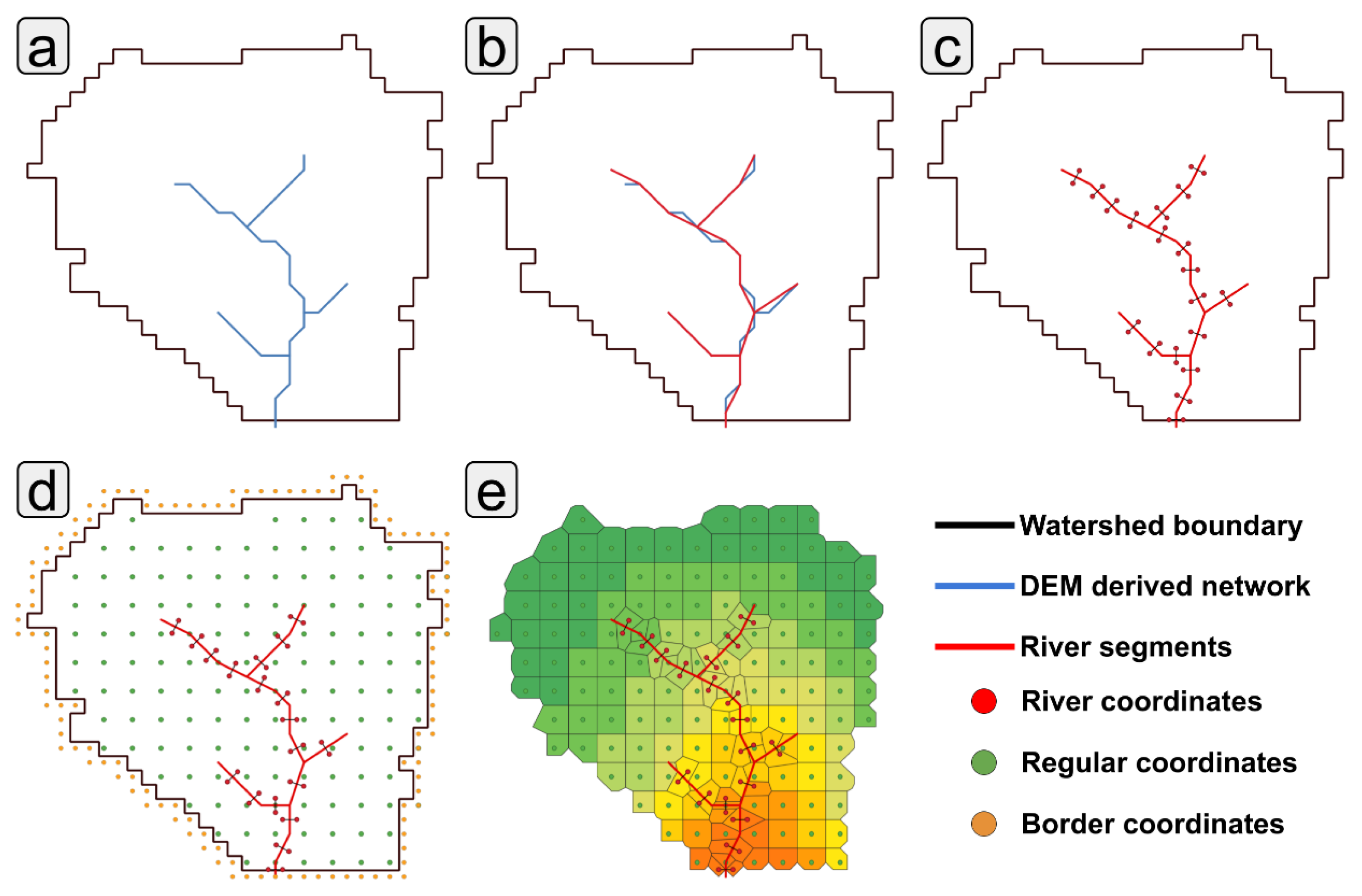
Figure 2.
Location of Bear Creek watershed.
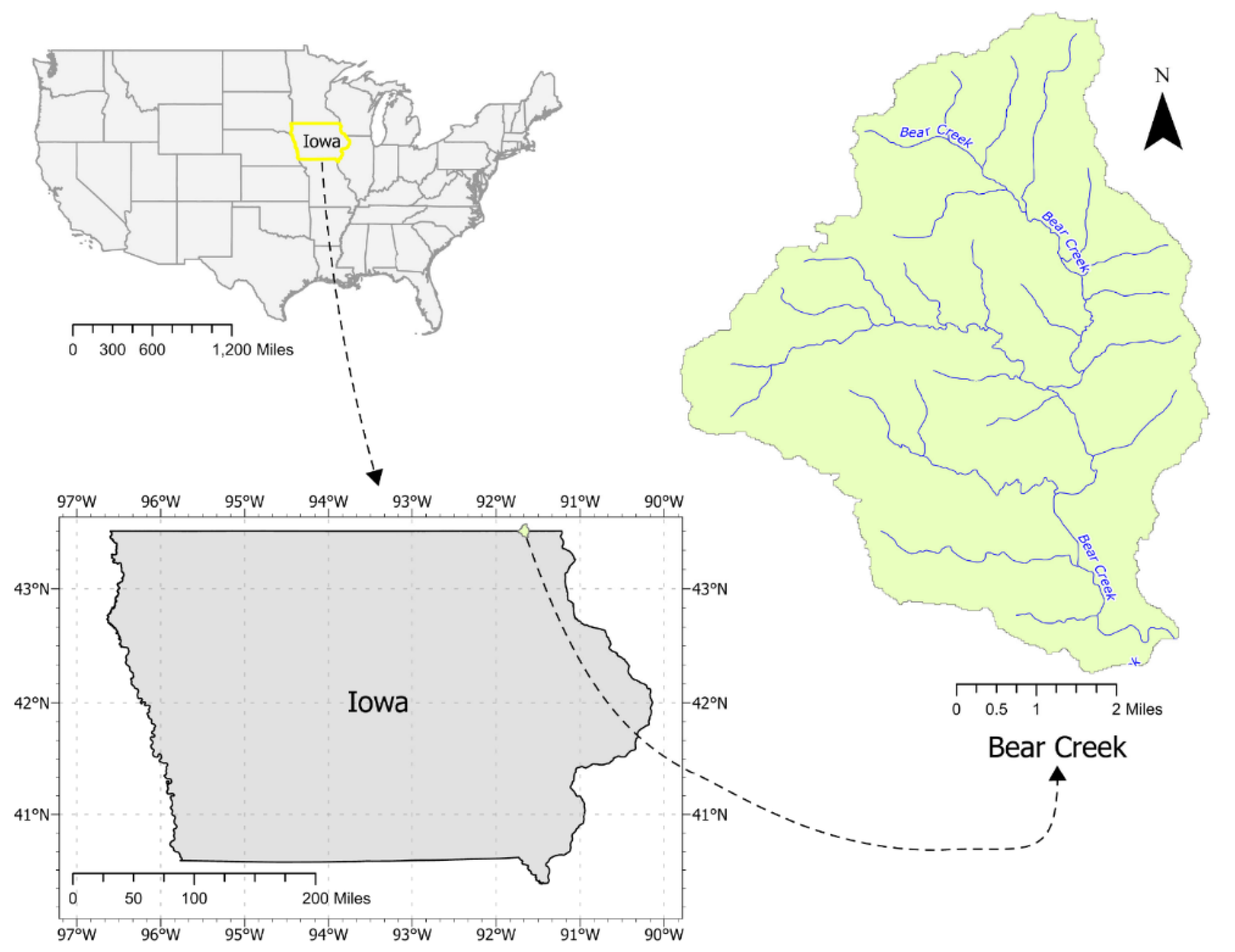
Figure 3.
a) Digital elevation model. b) Flow direction raster.
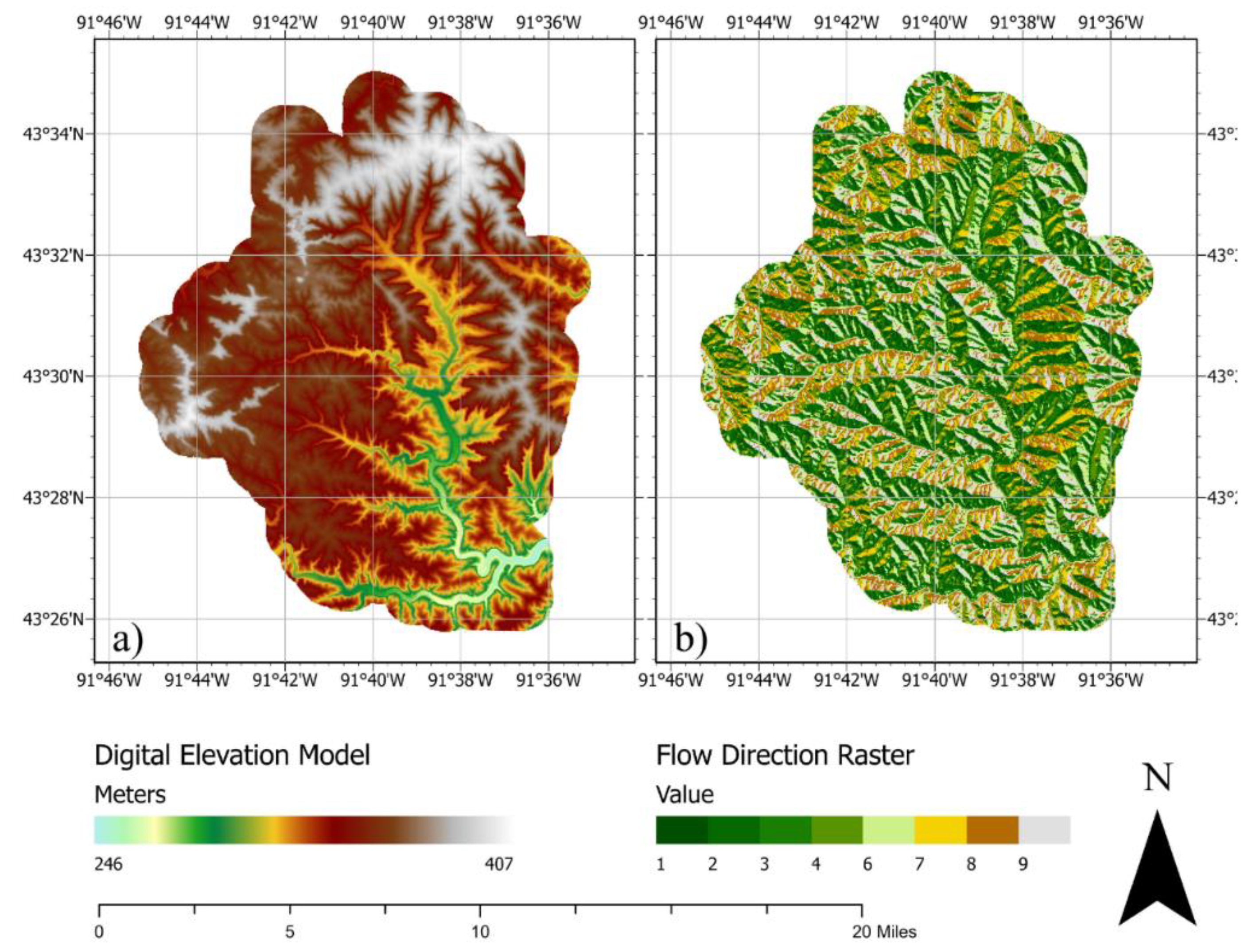
Figure 4.
Computational grids generated with GMesh. a) Mesh with a thousand elements, b) mesh with fifteen thousand elements, and c) mesh with thirty thousand elements.
Figure 4.
Computational grids generated with GMesh. a) Mesh with a thousand elements, b) mesh with fifteen thousand elements, and c) mesh with thirty thousand elements.
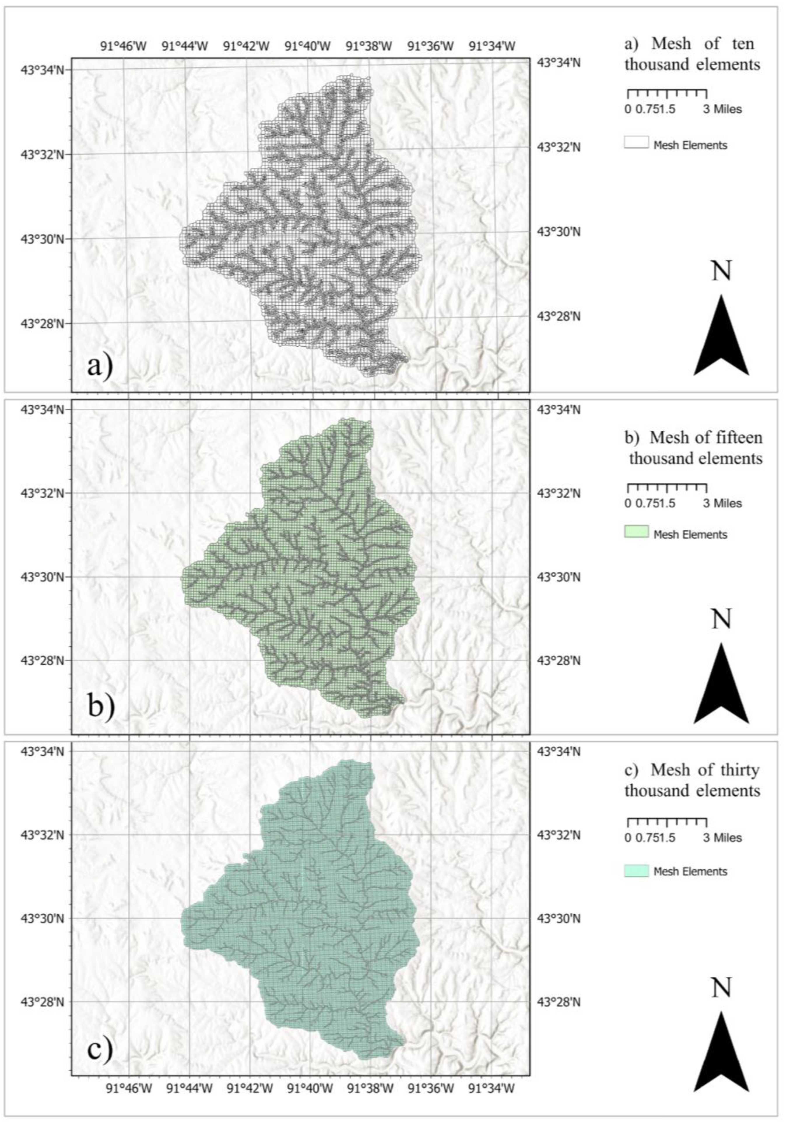
Figure 5.
GHOST simulation output hydrograph for each mesh resolution and zoom to the simulations between 3.5 and 4 days after the simulation starts.
Figure 5.
GHOST simulation output hydrograph for each mesh resolution and zoom to the simulations between 3.5 and 4 days after the simulation starts.
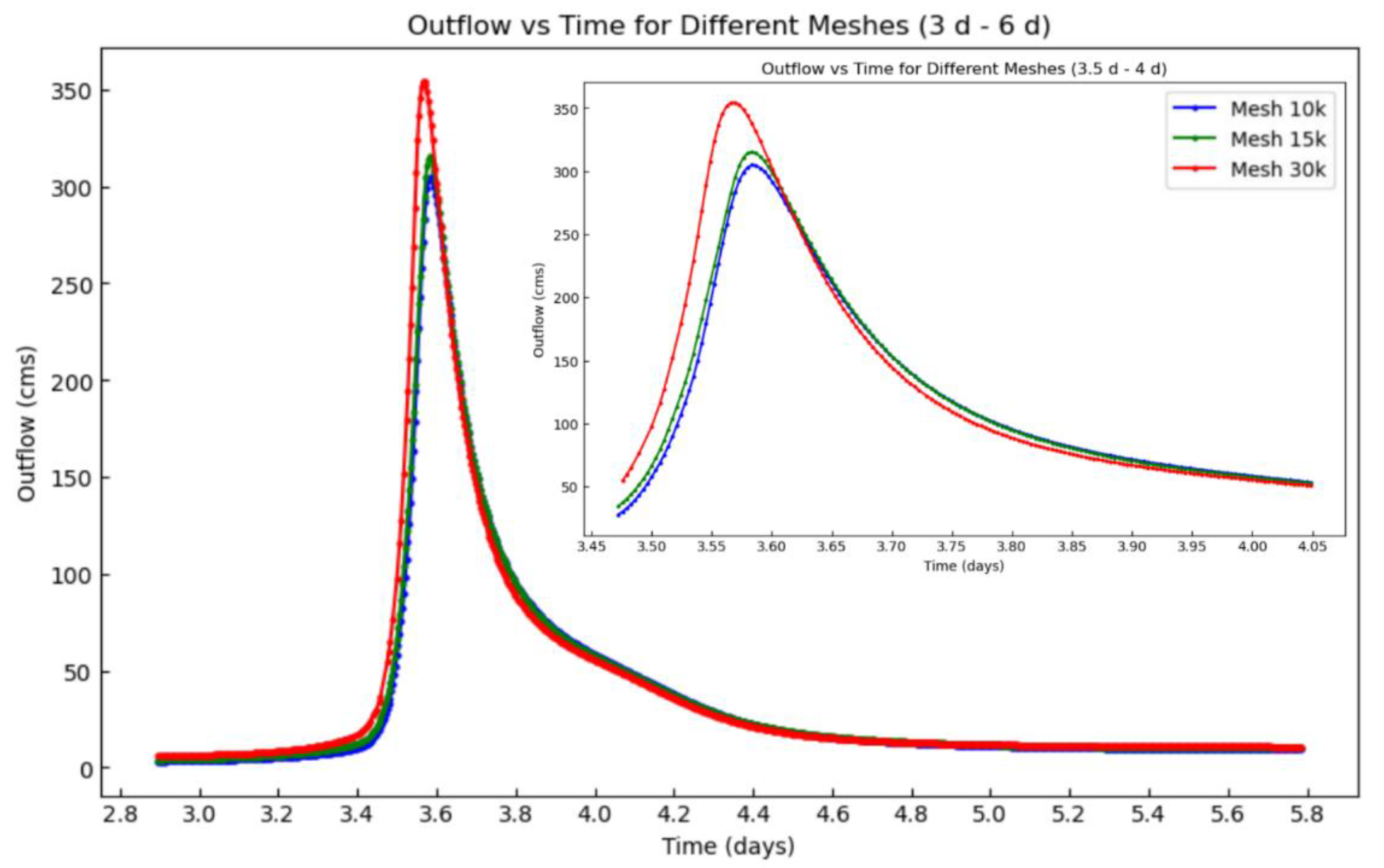
Figure 6.
Focus mesh generated using ghost_preprocess WMF module with ten thousand elements using focus module to create different size elements according with zones of interest inside the watershed (Zone 1= High refinement, Zone 2 = Low refinement, Zone 3= Medium refinement).
Figure 6.
Focus mesh generated using ghost_preprocess WMF module with ten thousand elements using focus module to create different size elements according with zones of interest inside the watershed (Zone 1= High refinement, Zone 2 = Low refinement, Zone 3= Medium refinement).
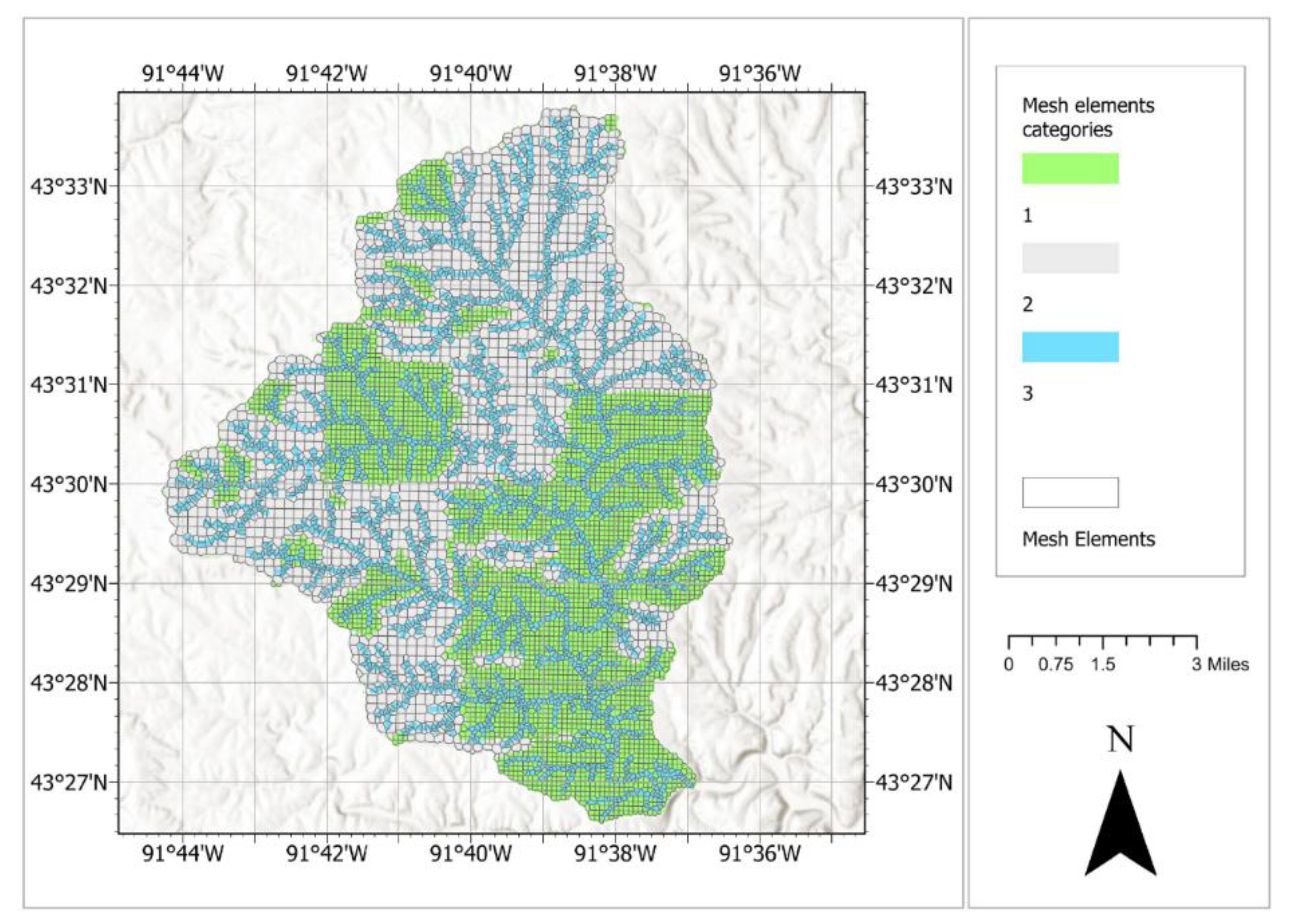
Figure 7.
GHOST simulation output hydrograph for Focus mesh generated using focus WMF module.
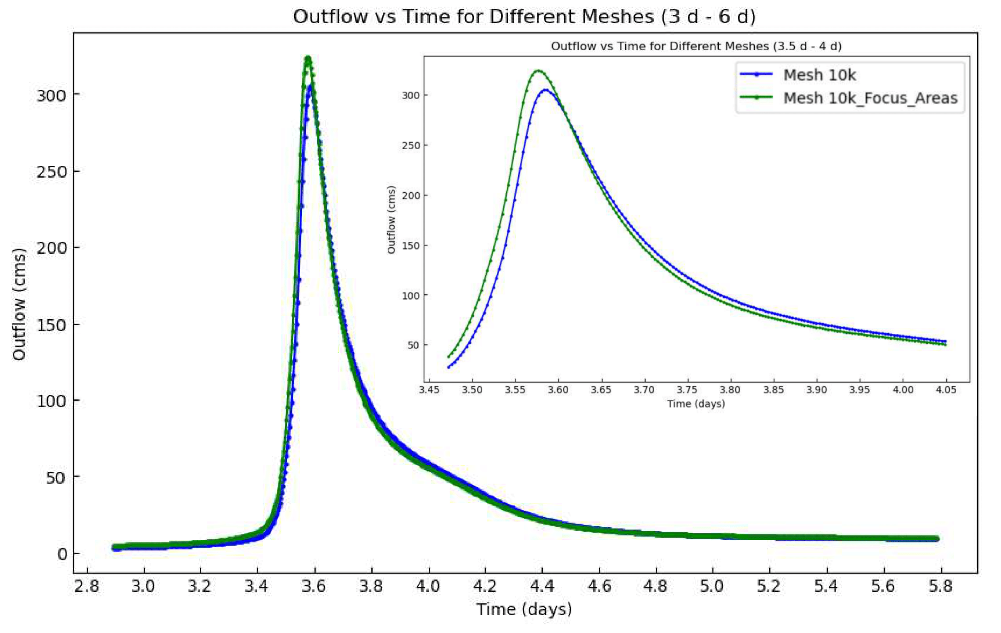

Table 1.
The computational time required to generate the mesh in the function of the number of elements.
Table 1.
The computational time required to generate the mesh in the function of the number of elements.
| Number of elements | Generation time (min) | Average number of faces |
|---|---|---|
| 10000 (10k) | 10 | 11 |
| 15000 (15k) | 20 | 8 |
| 30000 (30k) | 35 | 7 |
Table 2.
Computational time hydrological model according to the number of elements.
| Number of elements | GHOST computational time (hours) |
|---|---|
| 10000 (10k) | 0.5 |
| 15000 (15k) | 1 |
| 30000 (30k) | 7 |
Table 3.
Mesh generation and GHOST computational time for a configuration with around 10,000 elements and focus regions.
Table 3.
Mesh generation and GHOST computational time for a configuration with around 10,000 elements and focus regions.
| Item | Computational time (hours) |
| Mesh generation | 0.2 |
| GHOST execution | 0.4 |
Disclaimer/Publisher’s Note: The statements, opinions and data contained in all publications are solely those of the individual author(s) and contributor(s) and not of MDPI and/or the editor(s). MDPI and/or the editor(s) disclaim responsibility for any injury to people or property resulting from any ideas, methods, instructions or products referred to in the content. |
© 2025 by the authors. Licensee MDPI, Basel, Switzerland. This article is an open access article distributed under the terms and conditions of the Creative Commons Attribution (CC BY) license (http://creativecommons.org/licenses/by/4.0/).
Copyright: This open access article is published under a Creative Commons CC BY 4.0 license, which permit the free download, distribution, and reuse, provided that the author and preprint are cited in any reuse.


