1. Introduction
As an innovative ground transportation system, the maglev trains adopt the magnetic force to achieve contactless levitation, guidance and propulsion, successfully overcoming the problems faced by conventional trains, such as wheel-rail adhesion limitations, mechanical noise and wear and tear, etc [
1,
2]. They not only enrich the existing modes of transport, reducing the speed gap between trains and planes, but also becomes a green mode of transport with its high efficiency and environmentally friendly features. With the continuous progress of technology, the 200-300 km/h medium and low-speed maglev train has achieved commercial operation worldwide [
3,
4], which positioning and speed measurement engineering solutions have tended to mature [
5,
6].
However, for the 600 km/h high-speed maglev train, many technical challenges remain that are critical for safe and efficient operation [
7,
8]. At such high speeds, speed measurement and positioning become increasingly difficult. Sensor accuracy and fast signal processing are critical, as even small errors can lead to significant positional deviations. In the field of traction control, the challenge is to provide precise power control to deliver considerable traction without compromising system stability. Vehicle-to-ground communication also faces obstacles, as maintaining ultra-reliable, low-latency data exchange becomes more demanding as speeds increase. Meanwhile, levitation control is heavily influenced by small fluctuations in the magnetic field and the air gap between the train and the track, necessitating the implementation of highly sensitive and adaptive control strategies. In particular, the speed measurement and positioning technology is not only the basis for the closed-loop control of the traction and operation control system of the high-speed maglev train, but also the key to ensuring the safe and stable operation of the train [
9]. Therefore, the speed measurement and positioning technology of the high-speed maglev train is the focus of technological breakthroughs and technical application.
Because of the complexity of the operating environment of the maglev train and the high construction cost, it is particularly important to construct an efficient and reliable test environment at the early stage of the MPSS [
10]. The HIL semi-physical simulation technology provides an ideal solution for this purpose. It uses a real controller as the control unit, while the controlled object and the operating environment are presented in the form of a digital model, thus constructing a highly simulated HIL real-time simulation platform [
11,
12,
13]. HIL simulation technology has been widely used in the transportation field [
14,
15,
16]. Marinescu et al. [
17] used HIL simulation to validate electric vehicle charging algorithms. Simulating scenarios under controlled conditions reduces the negative impact of smart body learning on the grid. However, the scalability of this approach in more complex network environments remains to be fully explored. Yang et al. [
18] advanced the field by building a multiprocessor-based HIL platform designed for real-time simulation of train faults within a traction control system (TCS). The downside is that the integration of multiprocessor architectures may lead to increased system complexity and maintenance challenges. Zhao et al. [
19] utilized an HIL test system to validate the control strategy of a semi-active suspension system. The results confirmed the feasibility of HIL for performance evaluation, but the research did not address in depth the potential limitations of sensor accuracy under high electromagnetic interference (EMI) conditions. Bernal et al. [
20] applied the HIL technology to test a novel node architecture for wheel plane detection sensors. The feasibility of the sensor design was successfully explored without interfering with real-world operation, although further field validation is required to assess long-term reliability under different operating conditions.
The earliest applications of HIL simulation in maglev systems focused on the verification and optimization of control systems. In the late 1980s, the German Transrapid project [
21] pioneered the development of automated procedures for the analysis and design of nonlinear control systems. While this approach was innovative at the time, it encountered challenges in adapting to the rapidly evolving control requirements of modern maglev systems. Subsequent studies have further refined the application of HIL in this area. Wang et al. [
22] verified the effectiveness and feasibility of a velocity estimation scheme for vector-controlled linear induction motors (LIM) drives, especially for low and medium-speed maglev applications. Similarly, Hu et al. [
23] applied HIL simulation to evaluate LIM control algorithms, thus providing valuable reference data for traction control. However, both of these studies addressed LIM applied to maglev trains without focusing on the actual operation of the trains. Jandaghi et al. [
24] introduced a real-time digital simulation drive system based on FPGA technology for maglev applications. Their FPGA-based approach improves simulation accuracy and real-time performance, despite higher initial development complexity and cost. In addition, HIL technology has been extended to other key components of maglev systems, including operation control systems (OCS) [
25,
26], vehicle stability control [
27,
28] and TCS [
29,
30].
However, the application of the above HIL simulation technology is aimed at the operation control of the maglev train or the verification of the system function, and there is a lack of simulation platforms for the MPSS, especially for the high-speed trains over 600 km/h. Compared with traditional hardware-based testing solutions, HIL simulation does not require on-site testing or the construction of a complete physical system. By building a highly simulated real-time test platform, it greatly reduces the cost of testing and makes testing more targeted. In order to more intuitively show the innovative aspects of the HIL simulation platform proposed in this paper, several typical test solutions in the field of maglev trains are compared with it.
Table 1 shows the advantages of the proposed HIL platform in terms of cost, complexity and ease of implementation. In fact, there is no simulation test platform reported for MPSS. The HIL simulation platform proposed in this paper provides an effective solution for it. By simplifying the system integration and modular design approach, the system has lower complexity and is easier to implement. Subsequent experiments show that the platform can simulate multiple train operation modes with better performance in terms of flexibility and accuracy.
In this paper, an HIL simulation platform on the high-speed maglev positioning and speed measurement is reported to solve the related testing problems. Firstly, an absolute position detection method based on Gray-coded loops and a relative position detection method based on height compensation are proposed. The experimental results show that they effectively eliminate the cumulative error of positioning data during the operation of the maglev train, relative to the traditional rail transit positioning methods. Secondly, the generation methods of some key simulation signals, such as loop inducted signals and antenna pulse width modulation (PWM) signals in MPSS, are deeply analyzed. On this basis, the HIL simulation platform was built for testing the GSPU, which is the core of MPSS. The HIL simulation platform includes induction loops, transmitting antennas, power driver unit, FPGA simulator and host computer. This platform not only maximally simulates the operating environment, but also significantly reduces the cost and risk of on-site debugging. It provides a strong experimental support for the development of MPSS, and lays a solid foundation for subsequent system optimization.
2. Principle of Positioning
During the operation of the maglev train, the vehicle magnetic field interacts with the track magnetic field to generate a horizontal thrust that pushes the train forward [
31,
32]. To ensure that the train magnetic field is synchronized with the track magnetic field, and that the current frequency of the electromagnets on the track matches the train's operating speed, the traction system must acquire real-time and accurate information about the train's position [
33,
34]. Therefore, the MPSS plays a decisive role in the safe and efficient operation of magnetic levitation trains.
2.1. Composition and Principle of MPSS
In this paper, the MPSS is based on Gray-coded loops. The main reason for using Gray-coded loops is their unique error-reducing properties: since neighboring codes differ by only one bit, the risk of misinterpretation during signal conversion is greatly reduced. This is particularly beneficial in high-speed applications, such as 600 km/h maglev trains, where fast movements and environmental disturbances can easily lead to errors. In addition, the use of Gray-coded loops allows for the development of ground-based positioning and speed measurement, which greatly reduces the system's dependence on vehicle-to-ground communications. This not only enhances the measurement system's ability to withstand external interference, but also helps achieve millimeter-level positioning accuracy. By utilizing these advantages, the method improves the accuracy, continuity, and real-time performance of the system, making it a cost-effective and reliable solution for high-speed maglev train operations.
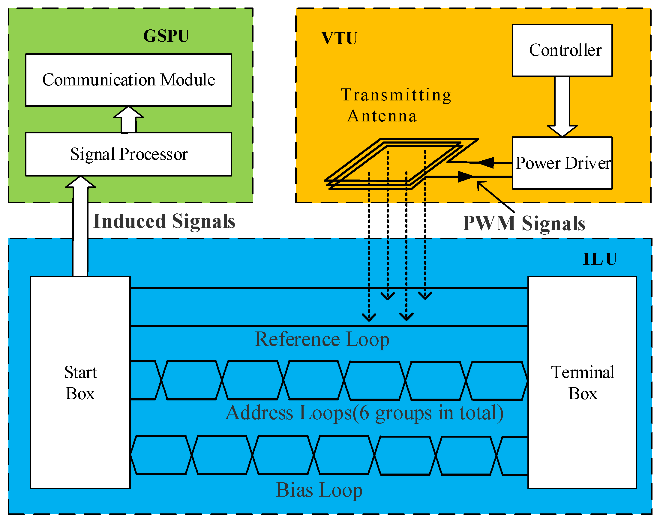
The MPSS consists of three parts: vehicle transmission unit (VTU), induction loop unit (ILU) and GSPU. In the VTU, the PWM signal generated by the controller is amplified by the driver and injected into the transmitting antenna. An alternating magnetic field is generated around it, and an voltage signal with the same frequency as the current frequency of the transmitting antenna is induced in the ILU. The induced signals is transmitted to the GSPU after the integration of the start box and the terminal box, and the GSPU gets the position and speed information of the train. Therefore, the core of the MPSS is GSPU, which is also the test object of the HIL simulation platform in this paper.The platform simulates a realistic operating environment by reconstructing induced signals and PWM signals. The structure of the MPSS is shown in
Figure 1.
The MPSS divides the positioning process of a maglev train into two stages: absolute position detection and relative position detection. The absolute position detection locates the train by positioning it within a Gray-coded period, while relative position detection further locates the train's precise position within that Gray-coded period. The combination of the two achieves the precise positioning of the maglev train. The speed of the train is then obtained by calculating the ratio of the distance
∆d between two adjacent crossings to the elapsed time
∆t:
2.2. Absolute Position Detection Based on Gray-Coded Loops
In the MPSS, a group of reference loop R and several groups of address loops Gn arranged according to the Gray code law are laid directly under the transmitting antenna of the train. The address loops cross once every certain step while the reference loop do not cross in the ILU. The number of address loops should be set according to the actual engineering requirements [
35], too many will lead to the problem of the induction signal attenuation, too few will lead to the GSPU setting distance is too close and increase the cost.
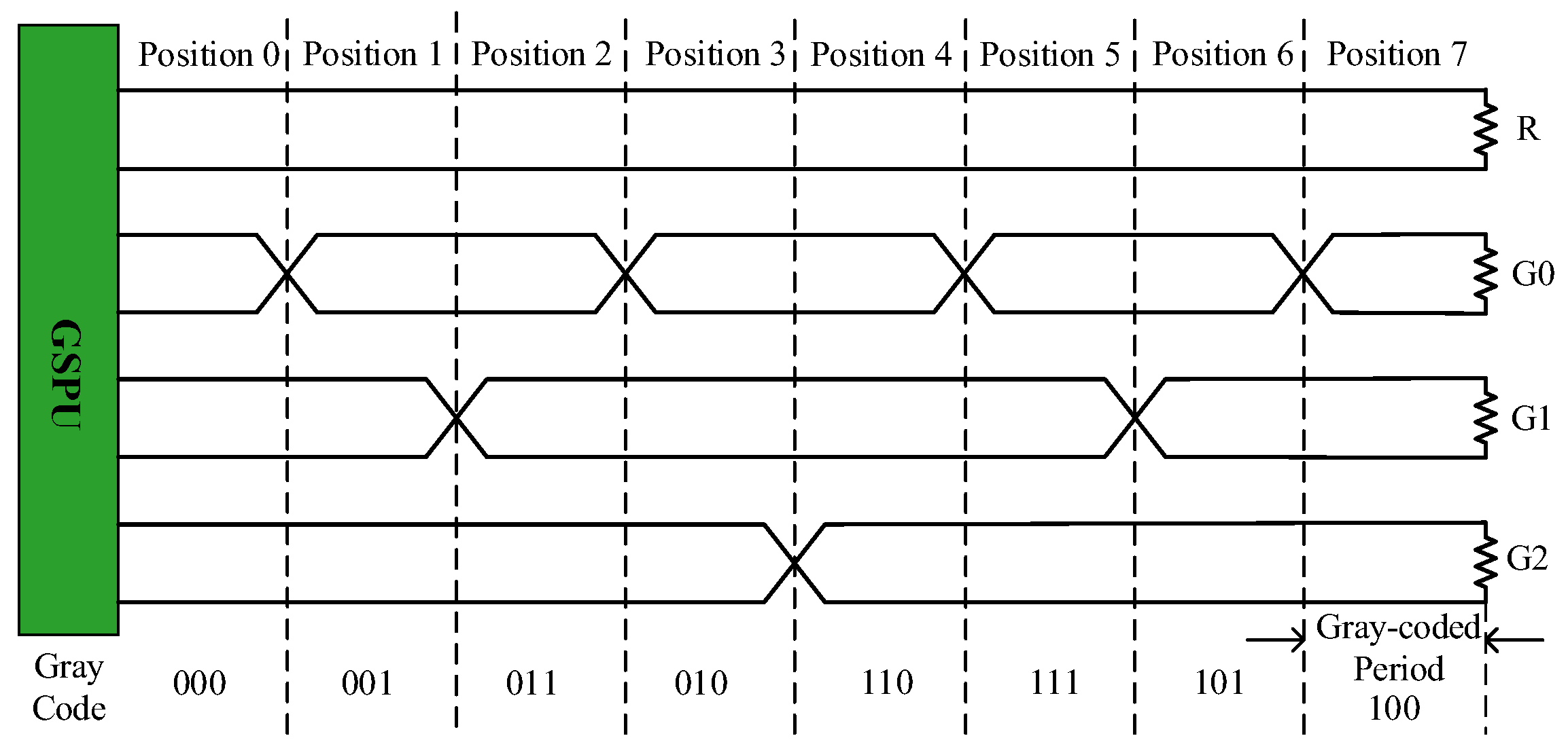
In this paper, we set up six groups of address loops, named as G0~G5. Since there are
codes for the six address loops, due to space constraints, a simplified explanation of its working principle with three groups of address loops are shown in
Figure 2.
When an alternating current is injected into the transmitting antenna, an alternating electromagnetic field is created around it. The address loops is approximately located in a uniformly distributed magnetic field [
36]. Each loop generates a corresponding induced signal which is sent to the GSPU. Since the reference loop is not crossed, its induced signal does not change with the position of the antenna. Instead, whenever the transmitting antenna passes through the cross node of the address loops, the phase of the induced signal changes by 180°. The voltage signals in the address loops are compared with the voltage signal in the reference loop, if the two are in the same phase, it represents the code ‘0’; if the two are in opposite phase, it represents the code ‘1’.
When the antenna is in position 0, the address loops G0, G1, and G2 have not passed through the cross node, and the phase of the induced signals is the same as that in the reference loop R. The Gray code for this position is ‘000’. When the antenna moves from position 0 to position 7, only one of the induced signals of the address loops is inverted. The corresponding Gray code also changes by only one bit, and the distance represented by one Gray code is a Gray-coded period. After decoding the Gray code to get the corresponding natural decimal number, the position of the train can be positioned within a Gray-coded period, thus completing the absolute positioning of the train.
2.3. Relative Position Detection Based on Height Compensation
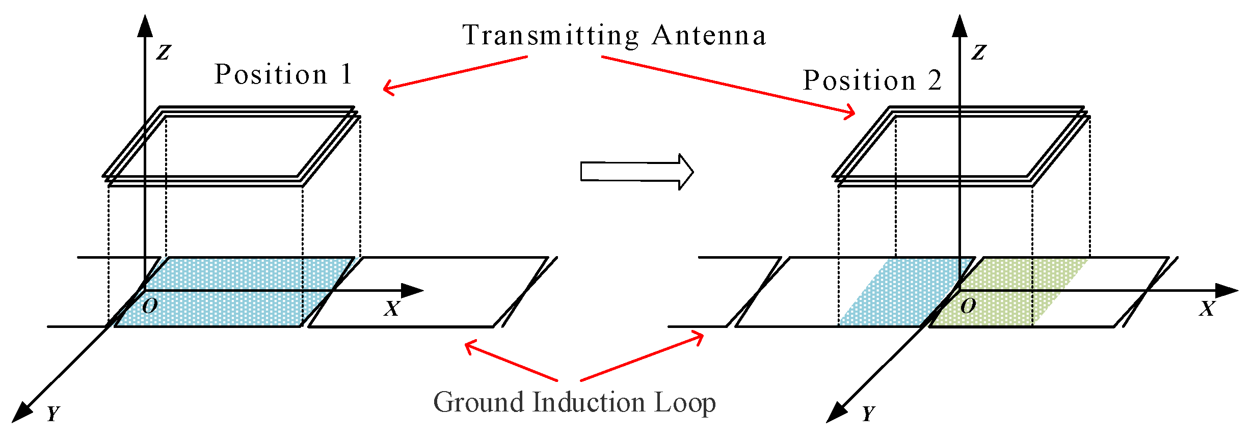
The relative position is detected based on the cyclic change of the induction signal, the principle of which is shown in
Figure 3, in which the ground induction loop is the lowest address loop G0. When the transmitting antenna moves to position 1, the effective induction area of the loop is the largest, and the magnetic flux that crosses the loop is the largest, so the amplitude of the induction signal is also the largest. When the transmitting antenna moves to position 2, the magnetic fluxes on both sides of the cross node are approximately equal, and the overall magnetic flux of the loop is approximately zero,so the amplitude of the induction signal is also close to zero. In the process of moving from position 1 to position 2. This means that the relative position of the transmitting antenna within a Gray-coded period can be exactly calculated according to the real amplitude of the induced signal.
However, the distance between the transmitting antenna and the sensing loop changes as the train travels on the track [
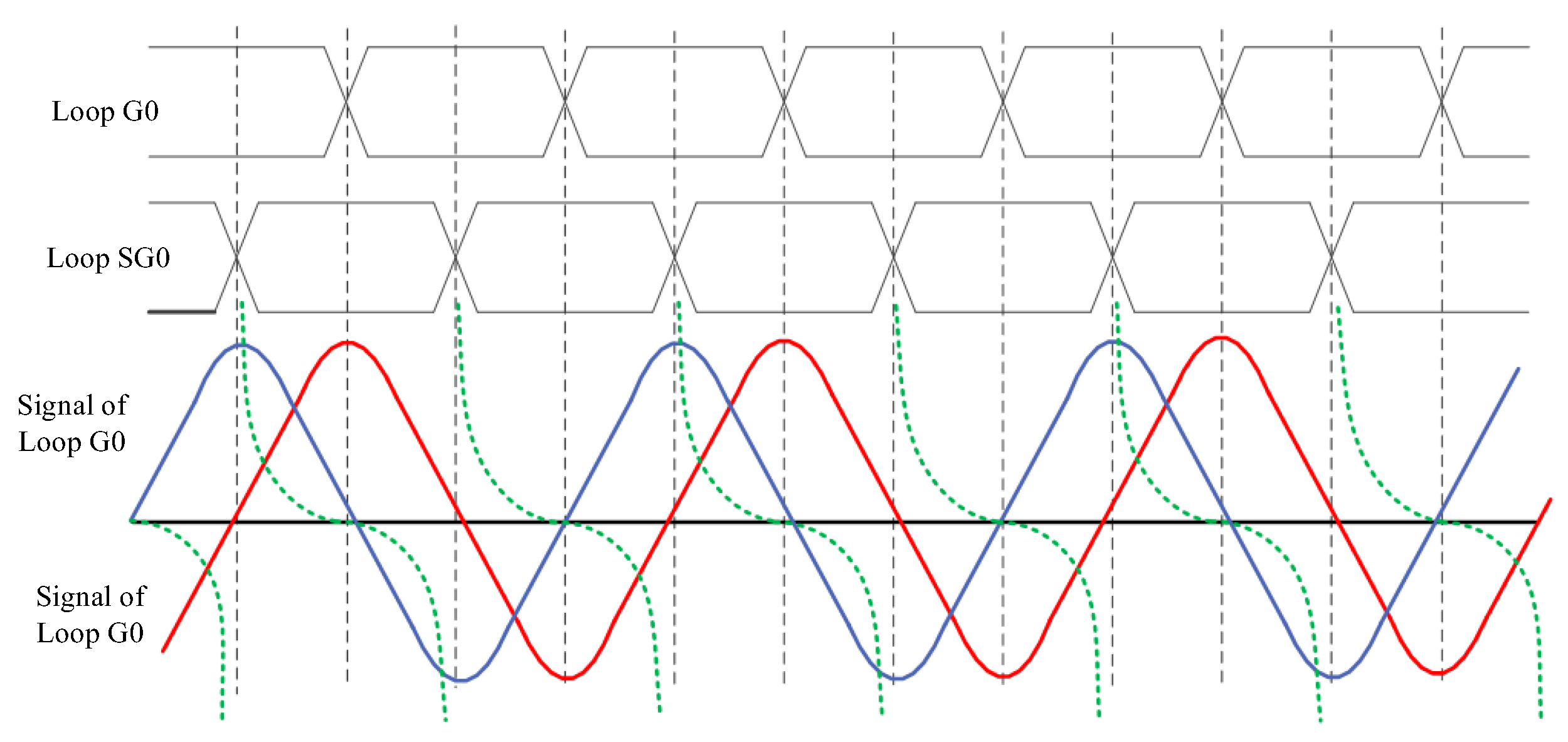
37], and the amplitude of the induced signal changes. This leads to an error in the inverse deduction of the relative position from the induced signal amplitude. To solve this problem, the bias loop SG0 for relative positioning is laid in this paper, which has the same structure and crossing cycle as the lowest address loop G0, but the loop cross node differs by half a crossing cycle, and the laying method of G0 and SG0 and their induced signal variations are shown in
Figure 4.
In
Figure 4, the phase ahead curve is the demodulated envelope of the G0 induced signal and the phase lag curve is the demodulated envelope of the SG0 induced signal, and the phase difference of the signals between them is 90 degrees, which can be expressed as respectively:
where
g(s) is the envelope signal at the standard height;
f(h) is a function related to the suspension height
h, which is linear in the range of suspension fluctuation;
s is the distance between the antenna and the starting point of the ILU; and
l is the Gray-coded period. To overcome the positioning error caused by the height fluctuation , the ratio of the amplitudes in the G0 and SG0 loops is calculated:
In Equation 4, the ratio depends entirely on the position of the train. It means that the influence of the train height fluctuation on the positioning accuracy is eliminated. In the actual operation, a complete mapping table of the ratios and relative position information was created, and the accurate relative position information can be easily obtained by indexing this table.
3. Signal Reconstruction Based on Parallel Signal Simulation
To simulate the real operating environment of GSPU, it is necessary to reconstruct some key signals, including the inductive signals of the loops and the PWM signals injected into the transmit antenna,etc. The HIL simulation platform is set up with eight groups of induction loops, which include a group of reference loop, six groups of address loops used for absolute position detection, and a group of bias loop used for relative position detection. In actual operation, these eight groups of induction loops receive signals with different amplitudes and phases.
Based on this, the simulation platform adopts a strategy of parallel signal simulation, and sets up a separate transmitting antenna for each pair of induction loops. When simulating train operation, the current parameters of each transmitting antenna are adjusted independently according to the real-time position of the train. This results in the simulation of the signals of the loops during train operation. Therefore, the relationship between the amplitude of the induction signal of the loop line and the train running position is analyzed in the following, and the control strategy of the PWM signal parameters of the transmitting antenna is determined.
3.1. Analysis of Induced Signal Amplitude and Train Position
Based on the principle of positioning and speed measurement of the induction loop, each position of the transmitting antenna corresponds to a unique induced signal amplitude. Therefore, to dynamically adjust the current magnitude of each transmitting antenna according to the simulated position of the train, a mathematical model describing the relationship between the induced signal amplitude of the loop and the position of the transmitting antenna is required.
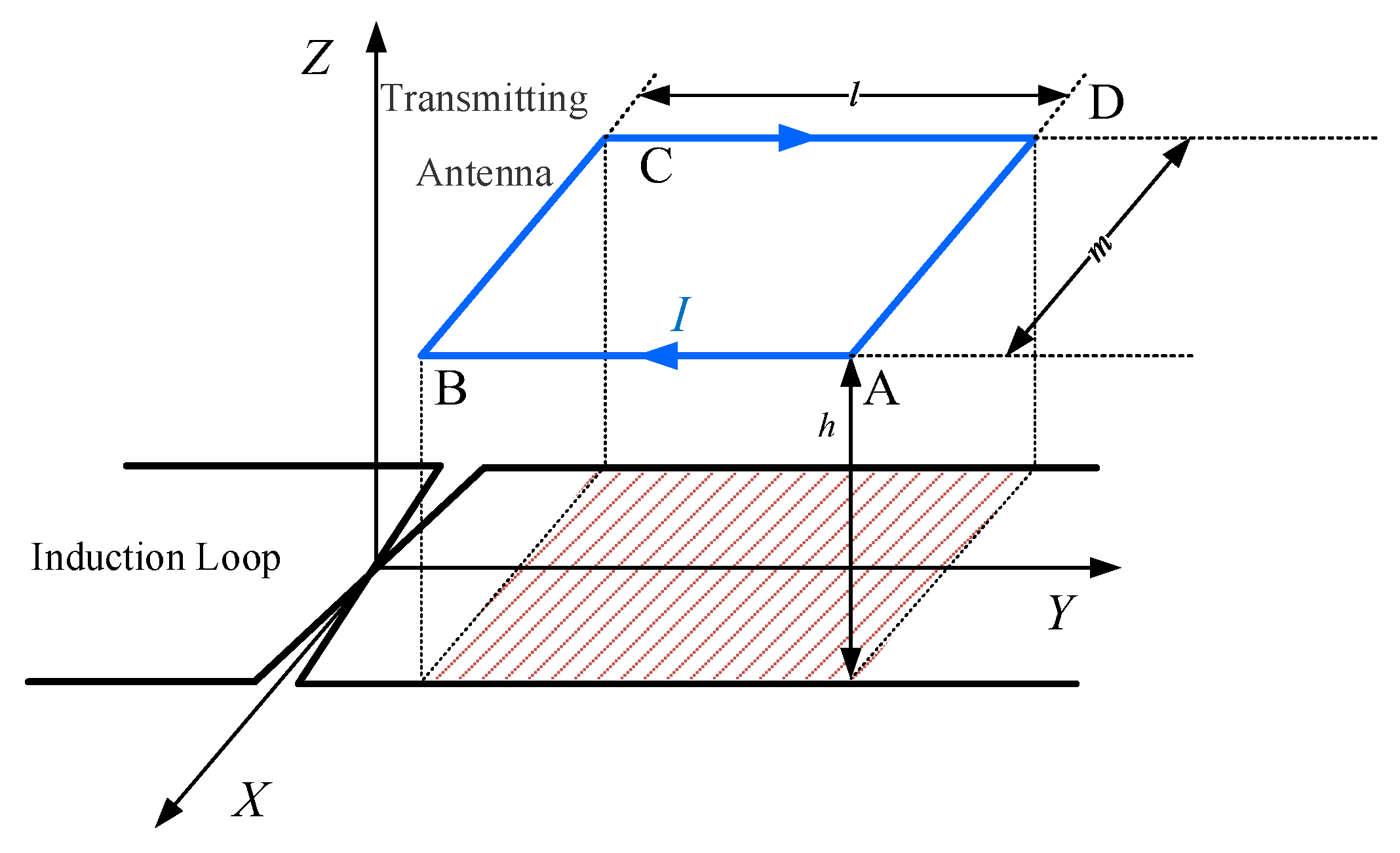
In practice, since the reference loop is not crossed, its induced signal amplitude remains constant during antenna movement, and thus only a fixed current needs to be injected into the corresponding transmitting antenna. As for the address loops and the bias loop , they can be grouped into the same category for discussion.Further, taking the lowest address loop G0 as an example,
Figure 5 shows the positional relationship between the transmitting antenna and it.
Both are of equal width, and the transmitting antenna is wound by a multi-turn coil in a rectangular shape. Considering that the strength of the magnetic field outside the closed coil decays rapidly and the transmitting antenna is close to the induction loop, the effective area of the magnetic field across the induction loop can be approximated as the projection of the transmitting antenna in the loop. Consider that the transmitting antenna is a single-turn coil consisting of segments AB, BC, CD, and DA. The magnetic induction at any point
P(x,y) consists of the superposition of the magnetic fields produced by these four electrified wires. The expression for the magnetic induction at point P was obtained as follows:
where
is the vacuum permeability,
I is the current injected in the wire,
m is the width of the transmitting antenna, and
is the length of the transmitting antenna.
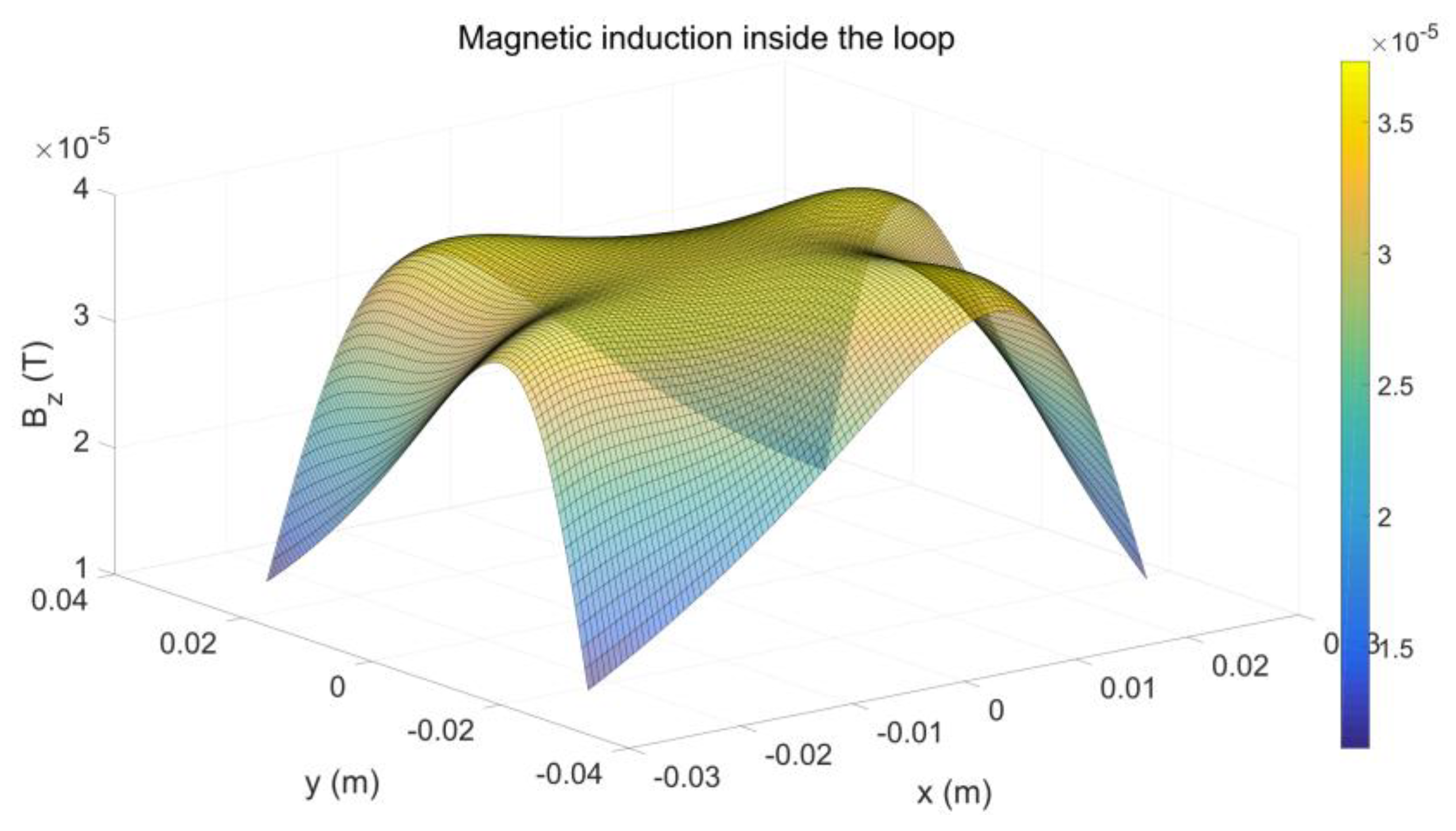
Since the induction loop is laid horizontally, the induced signal is mainly determined by the induced electromotive force generated by the change in magnetic flux across the plane of the loop. Therefore, the main focus is on the Z-direction component of the magnetic field. By superposing the z-direction components of the magnetic induction strength generated by each segment of the wire, an expression for the total z-direction component of the magnetic induction strength is obtained:
by bringing Equation 5, Equation 6, Equation 7, and Equation 8 into the above equation, it is obtained:
According to the Equation 10, assuming that a 5A current is injected through a square transmitting antenna with a side length of 5cm, the z-direction distribution of the magnetic induction is shown in
Figure 6 at a horizontal plane with a distance of 2cm from the antenna.
Figure 6 shows that the magnetic field is approximately uniformly distributed within the projection of the induction loop.
According to the law of electromagnetic induction, the magnitude of the induced electromotive force
e generated in a conductor loop is proportional to the rate of change
/
of the magnetic flux through the loop, i.e:
according to the conclusion that the vertical component of the magnetic induction intensity inside the induction loop is approximately uniformly distributed, the equation 11 can be simplified as:
In Equation 12, with a constant magnetic field generated by the transmitting antenna, the induced signal of the loop is only related to the effective projected area of the transmitting antenna in its plane. And the amplitude of the induced electromotive force is directly proportional to the movement distance of the antenna during a loop crossing cycle. Further, assuming that the distance between the centre of the transmitting antenna and the nearest loop crossing point is d. The crossing cycle of the induction loops is l . The relationship between the peak-to-peak value of the induced voltage and d can be expressed as:
3.2. Analysis of Antenna Resonant Current and PWM Signal Duty Cycle
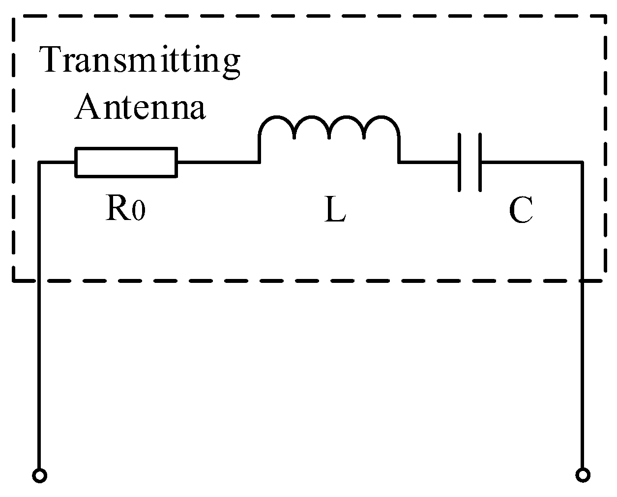
During the actual operation of the train, the amplitude of the induced signal in the loop will change periodically with the movement of the transmitting antenna, so the induced signal received in the corresponding loop can be simulated by adjusting the current of the transmitting antenna. The transmitting antenna is connected in series with a capacitor to form an RLC resonant circuit, and the circuit model can be approximated by the circuit of
Figure 7.
The center frequency of the resonant circuit is the same as the frequency of the PWM signal which is used as the excitation, and the current resonance of the circuit can be made by injecting the PWM signal into the circuit. By adjusting the duty cycle of the PWM signal, the magnitude of the resonant current in the transmitting antenna can be changed, thus changing the magnitude of the magnetic field generated by the transmitting antenna. To simulate the real operating conditions, the relationship between the resonant current amplitude and the duty cycle of the PWM signal is analyzed according to the RLC resonant circuit model.
For a periodic signal
f(t) with period
T , it is expressed as:
This periodic function can be extended to an infinite series using trigonometric coefficients:
i.e.
The Fourier transform of the periodic signal f(t) is obtained by solving for according to the Fourier series expansion formula.
The PWM signal is used as the excitation source of the transmitting antenna, which is injected into the transmitting antenna and resonates to produce a high-frequency sinusoidal current signal in the antenna. The relationship between the amplitude of the resonant current and the duty cycle of the PWM signal is analyzed below. Let the PWM signal be a square wave signal with period T and duty cycle
α:
substituting into the expansion formula gives:
In Equation 18, the fundamental wave amplitude is the largest. Since the RLC series resonant circuit is a band-pass filter, if the fundamental frequency of the square wave is equal to the centre frequency of the circuit, a resonant current of this frequency is generated between the inductor (i.e., the transmitting antenna) and the capacitor. The amplitude of this resonant current
|A| is related to the PWM signal as:
where
A is the peak-to-peak value of the square wave signal and
α is the duty cycle of the square wave signal.
Q is the amplification (quality factor) of the RLC series resonant circuit, which is related to the circuit parameters. Therefore, the amplitude of the sinusoidal voltage in the transmitting antenna is sinusoidally related to the duty cycle of the PWM signal. The change in voltage amplitude in the transmit antenna can be adjusted by adjusting the duty cycle.
4. Implement of the HIL Platform
This HIL simulation platform is designed to validate the GSPU. The core task of the platform is validating the function and reliability of the GSPU by simulating the induced signal of the ILU when the train is in actual operation. In addition, the platform needs to have the ability to flexibly set the train operating parameters, so as to simulate the signals received by ILU under different operating conditions, and to enhance the wide applicability and practicality of the simulation test.
4.1. Platform Structure Design
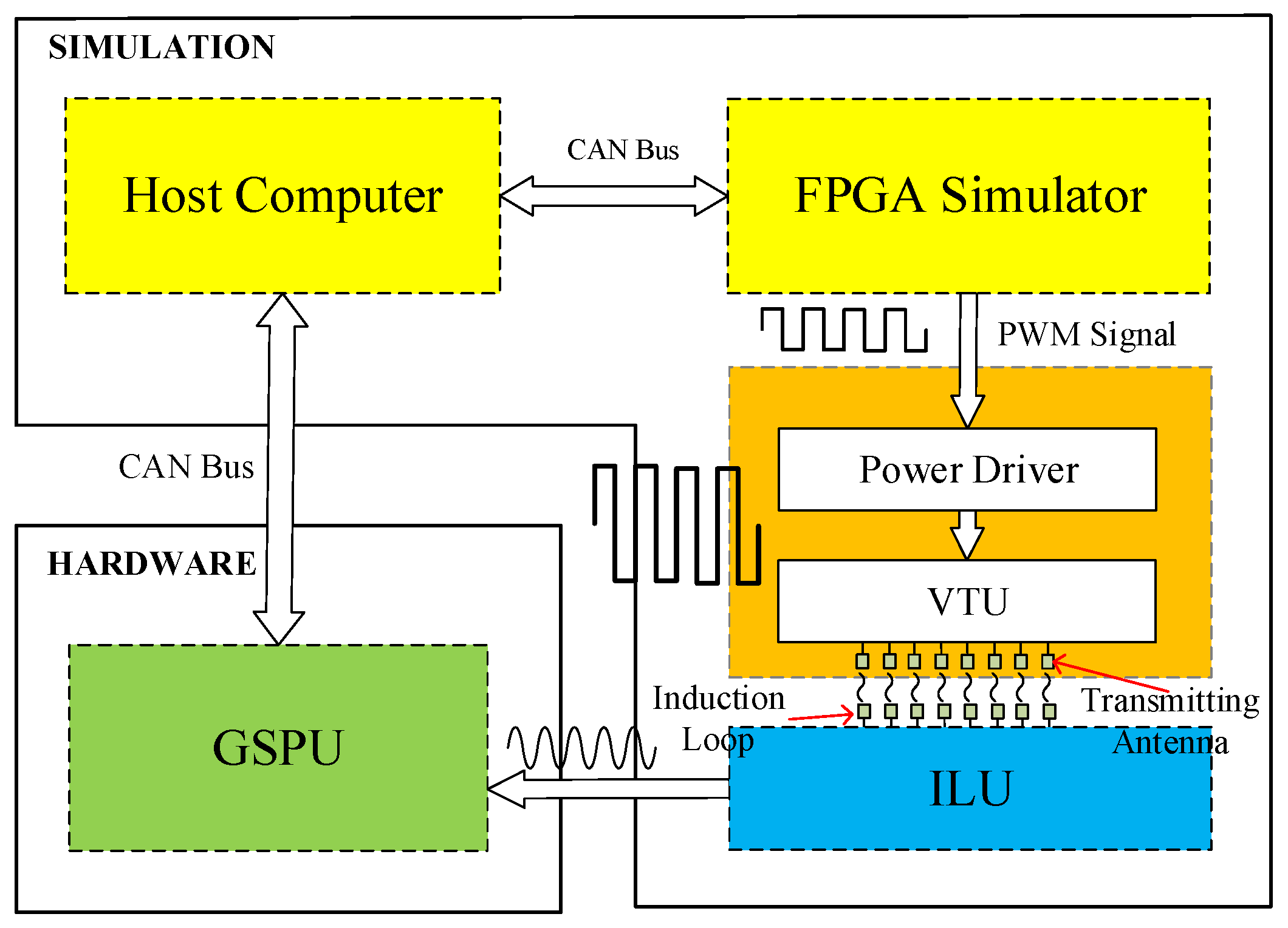
The HIL simulation platform is composed of a host computer, an FPGA simulator, a resonant circuit, and the ILU, while the test object is the real GSPU. The platform is designed with eight groups of induction loops, each paired with a corresponding transmitting antenna, as illustrated in
Figure 8. This multi-loop arrangement allows for spatially distributed signal generation, which is crucial for accurately mimicking the electromagnetic environment along the maglev track.
Firstly, the simulation begins with the host computer, where parameters such as the train's running mode, speed, acceleration, and other relevant dynamic conditions are preset. The FPGA simulator then uses these control parameters to compute the train's instantaneous position in real time. This computation is essential for simulating realistic operational conditions and ensuring that the subsequent signal processing reflects actual train dynamics.Based on the calculated running position, the FPGA simulator computes the induced voltage signal for each induction loop in real time by applying Equation 13. This calculation considers the geometric and physical properties of the loops as well as the varying train position, ensuring that the simulated signals closely replicate those that would be generated in a real environment.
Following the signal computation, the platform adjusts the PWM signal duty cycle for each transmitting antenna according to Equation 19. These PWM signals, once processed by the power driver, are injected into the VTU to simulate the induced signals that would be received by the ground-based loops. The proper calibration of these signals is vital for ensuring that the simulated electromagnetic fields accurately represent the conditions encountered by the GSPU.
The real GSPU, acting as the hardware under test, receives these simulated induced signals from the loops. It processes the data to extract critical information such as the relative and absolute position of the train and its running speed. The GSPU then transmits the processed information back to the host computer via the CAN bus, thereby completing the closed-loop system. This real-time feedback mechanism is instrumental for validating the performance and reliability of the system under simulated operating conditions.
4.2. Platform Hardware and Software Design
The hardware of this platform includes an FPGA simulator, a power driver and a VTU. The simulator is responsible for controlling each antenna, which requires high parallel computation capability. Therefore, the processing unit of the simulator adopts an FPGA. The simulator's input is the simulated running position of the train, provided by the host computer, and its output is the PWM signal used to control the transmitting antennas.The power driver amplifies the PWM signal generated by the simulator, which is used to drive the transmitter antennas to generate high frequency alternating current.
The software of this platform includes the host computer and the FPGA program of the processing unit in the simulator. The host computer uses a graphical display interface to control the start, pause and stop of the simulation process, and the train motion can be set directly in the interface. The FPGA simulator calculates the train position in real time according to the train operation parameters. The simulation platform mainly simulates three typical train operation modes, including instantaneous position mode, instantaneous speed mode and acceleration mode. The model needs to be implemented in FPGA, so it needs to be represented by differential equations to calculate the position and speed of the train in real time.
In the host computer, parameters such as train operation mode, operation speed
, acceleration
a, operation position
can be set. These parameters are given to the FPGA simulator through the CAN bus. The following is an example of acceleration mode to give the differential equation of the running position of the train. In the accelerated motion mode, the train starts from position 0, does uniformly accelerated linear motion with the given acceleration
a, and reaches the given maximum speed
to keep the speed unchanged to do uniform linear motion. The differential equation with respect to the train running position
is expressed as:
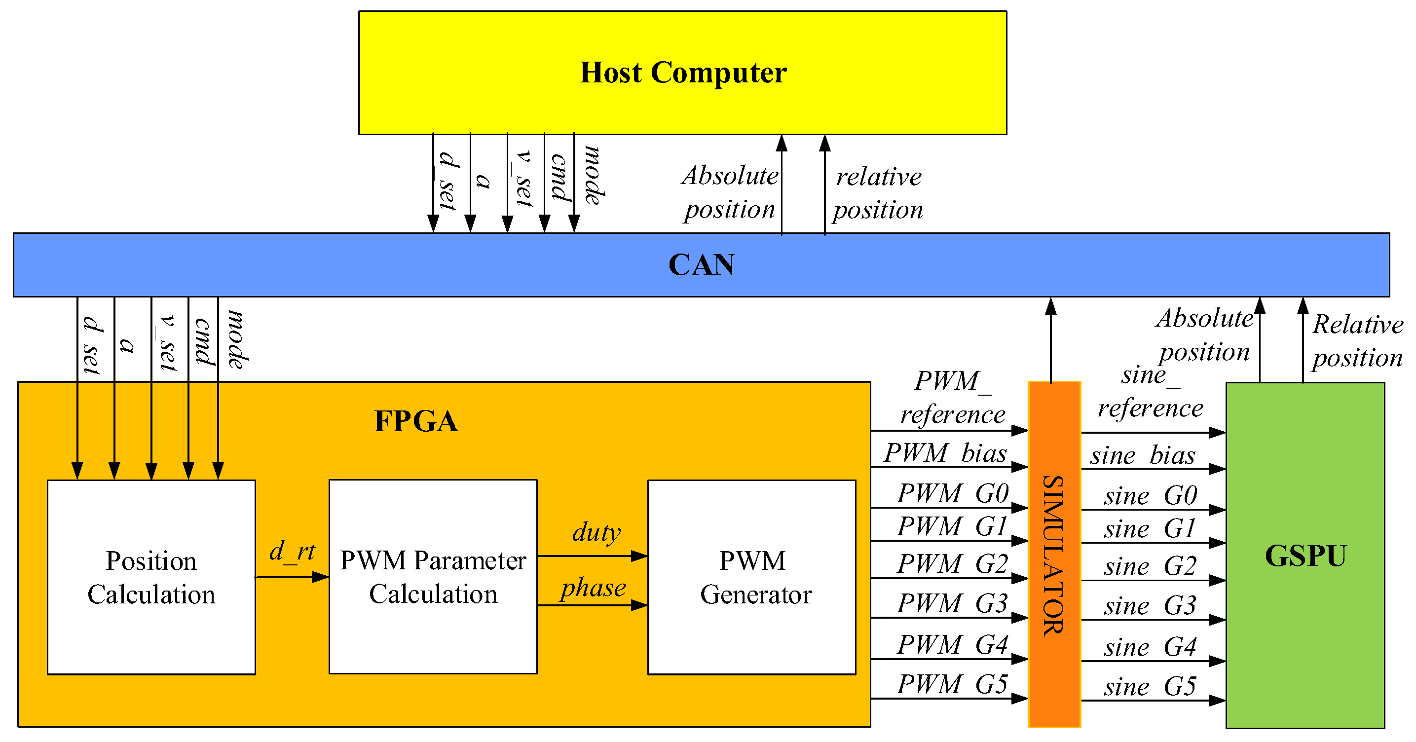
The operation of the simulation system is shown in
Figure 9. The train operation mode and parameters are set in the host computer, and the FPGA reads these parameters through the CAN bus and solves the above differential equation in the Position calculation module to obtain the real-time running position of the train,
d_rt. The PWM parameter calculation module calculates the
duty cycle and
phase of the PWM wave of each transmitting antenna according to
d_rt. At the same time, the host computer centrally displays the simulated running position and the position information processed by the GSPU. The relative position, absolute position and the Gray code are displayed in the form of curves in the host computer interface. By comparing whether the two are consistent or not, it can be verified whether the processing function of the ground unit is correct or not. The host computer can also save the simulation data to further analyse the operation of the GSPU.
5. Results
To evaluate the effectiveness of the proposed HIL simulation platform, a series of experiments were conducted focusing on the physical implementation and functional verification of the system. This section presents the results obtained from the constructed platform and analyzes the performance of the GSPU under different operating conditions.
5.1. Physical Construction of Platforms
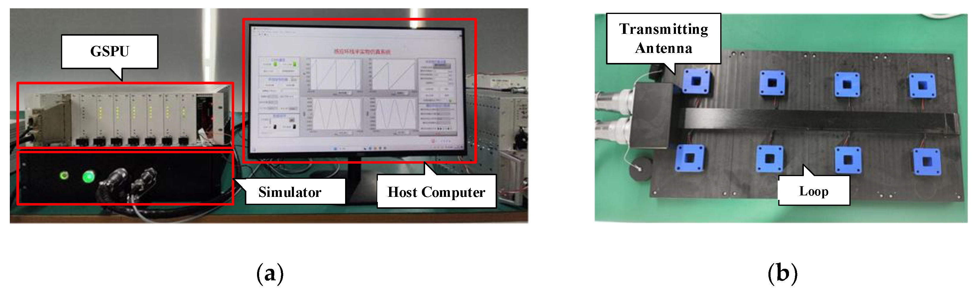
The HIL simulation platform consists of four parts, which are host computer, simulator, real GSPU chassis and signal receiving unit. Among them, the signal receiving unit includes eight transmitting antennas and eight groups of induction loops, as shown in
Figure 10.
The HIL simulation platform is run in instantaneous speed mode, instantaneous position mode, and acceleration mode, respectively. The corresponding parameters are shown in
Table 2.
Table 3 shows the resource occupancy of different software modules in the FPGA. It shows that the communication module occupies the highest resource occupancy, and the calculation and generation of the PWM signal parameters of the transmitting antenna occupies a smaller resource occupancy, indicating that the simulation strategy based on parallel signal simulation is effective.
5.2. Functional Verification
5.2.1. Instantaneous Speed Mode Analysis
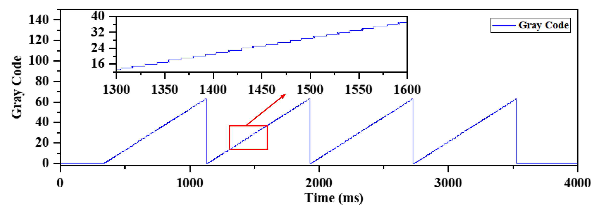
In the instantaneous speed mode, the train starts from position 0 and moves at a constant speed according to the set running speed. The relative position and absolute position information processed by the GSPU can be observed in the host computer interface. To facilitate the display of the absolute position, the GSPU decodes the Gray code into BCD code and finally displays it in the form of decimal in the host computer interface.
Figure 11 shows that the Gray code information of the train position is incremented from 0 to 63 and then becomes 0 again, and keeps cycling as expected. Each Gray code then corresponds to a Gray-coded period of the ground loop to represent the absolute position of the train.
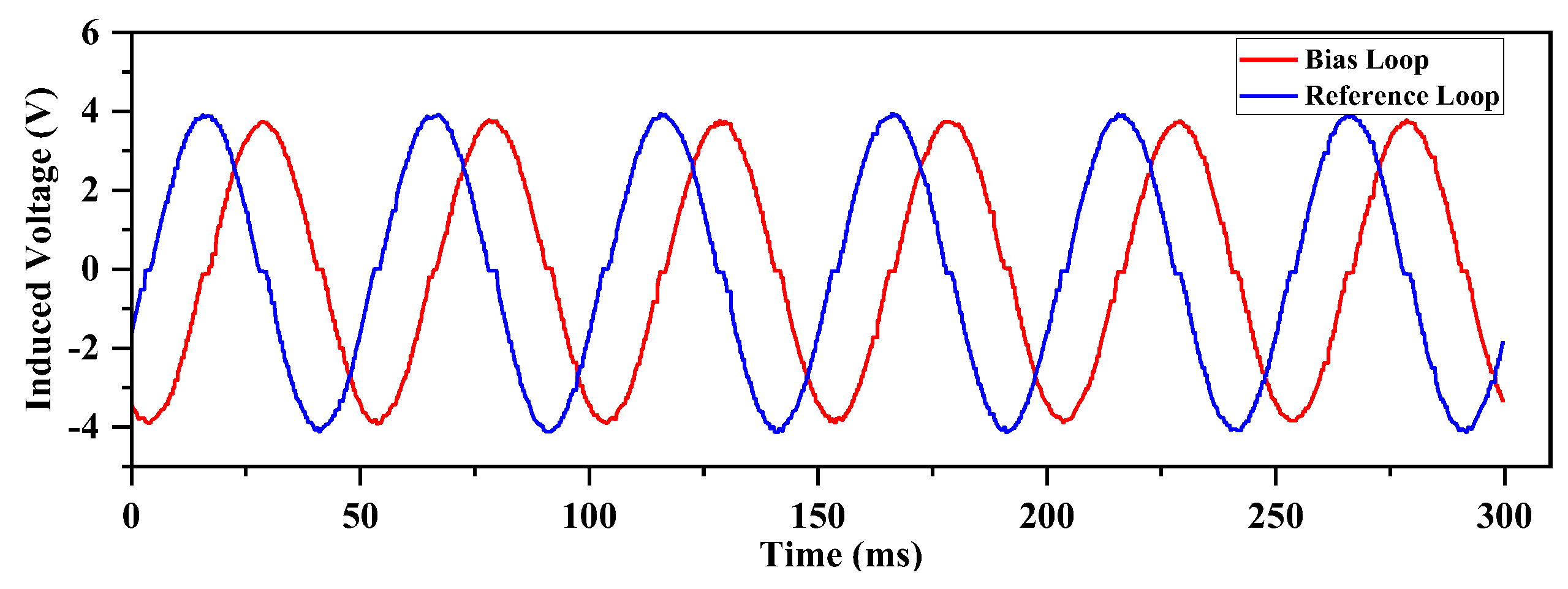
The relative position is calculated based on the division of the amplitude of the induced signal of the lowest address loop G0 and the bias loop SG0. The amplitude of the G0 and SG0 induced signals output from the GSPU is shown in
Figure 12, which is approximated as two sinusoidal signals with a phase difference of 90°.This is consistent with the results analyzed in
Figure 4.
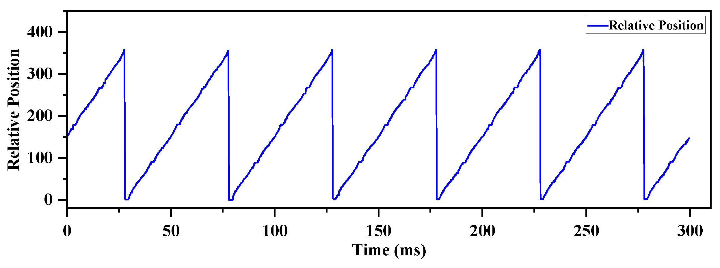
The relative position change curve obtained from the processing of the G0 and SG0 induced signals is shown in
Figure 13. The curve approximates a sawtooth wave and varies between 0 and 360°, indicating the relative position change of the train within a loop cell as expected.
According to the absolute position and relative position information obtained from the processing, the running position can be calculated. Comparing with the simulated distance and speed sent by simulator, it is found that the two are consistent, which indicates that the HIL simulation platform can correctly simulate the operating environment of the GSPU.
5.2.2. Instantaneous Position Mode Analysis
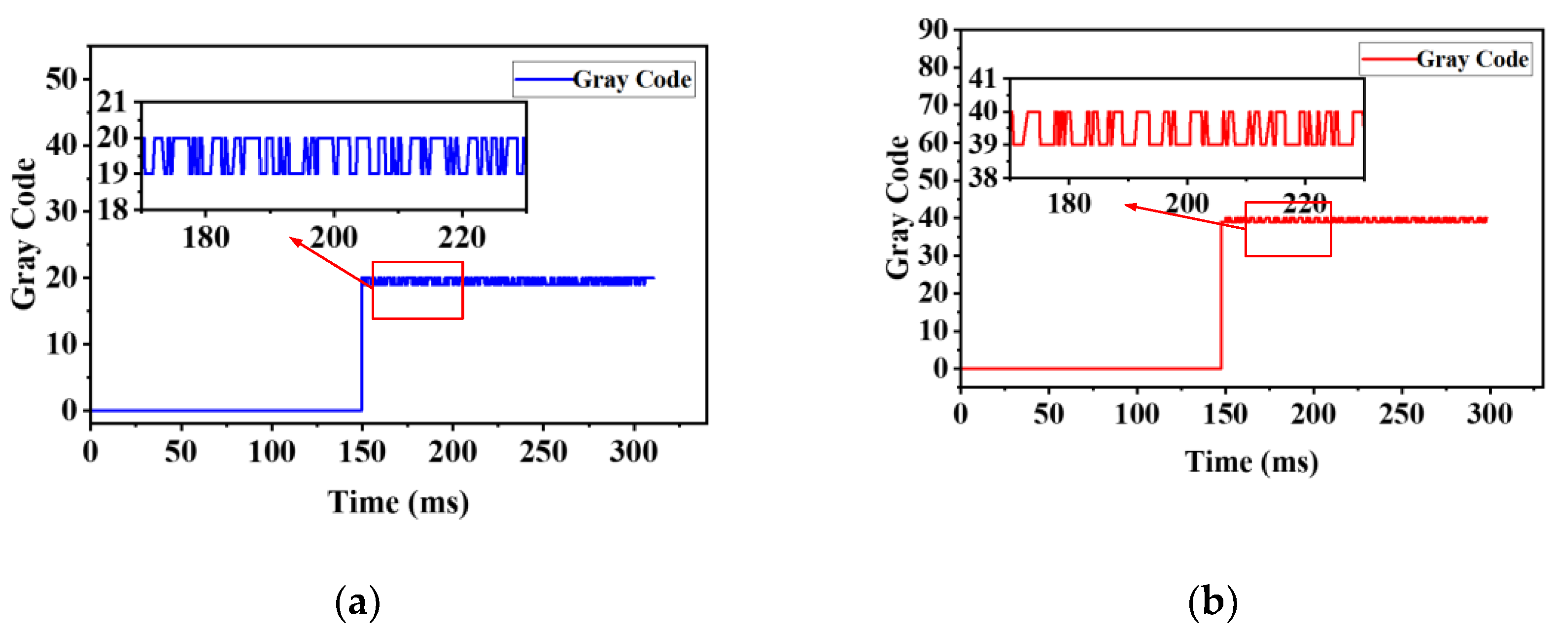
In the instantaneous position mode, the stationary position of the maglev train is set. When the position is set to 1000 mm and 2000 mm respectively, the absolute position information is shown in
Figure 14. As the Gray-coded period of the loops is 50 mm, when the train is at 1000 mm, it is located at the 20th Gray code of the loop, i.e. the BCD code corresponding to the absolute position Gray code is 20. As the train is directly above the crossing point of the loop, the absolute position code jumps between 19 and 20. Similarly, when the train is at 2000 mm, the absolute position code jumps between 39 and 40, as expected.
5.2.3. Acceleration Mode Analysis
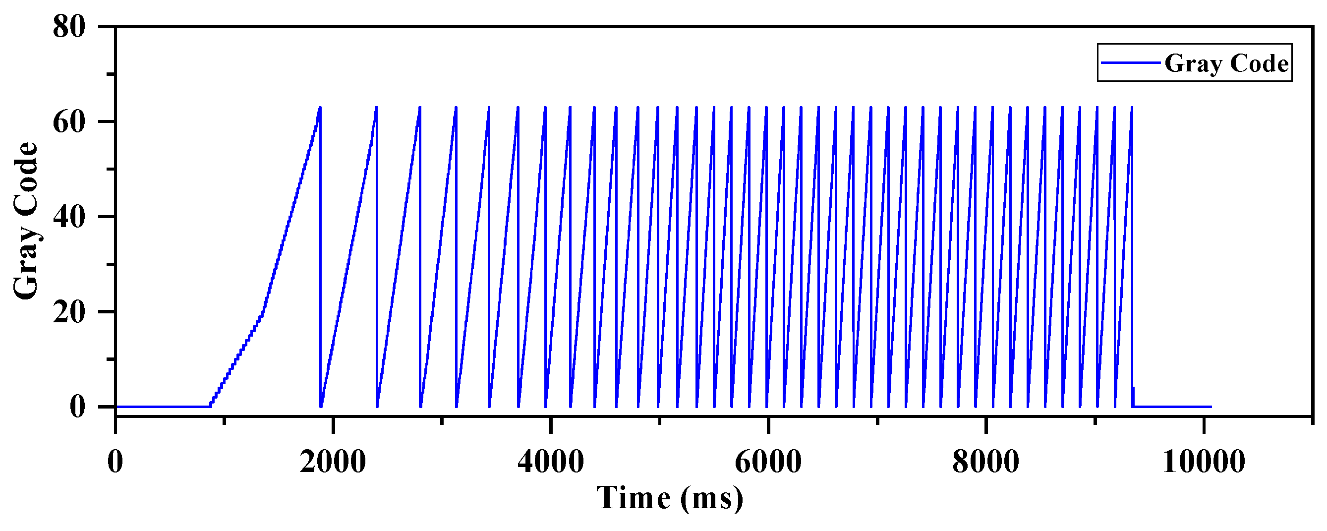
In acceleration mode, the maglev train starts from position 0, accelerates uniformly with an acceleration of
, and runs at a uniform speed after the speed reaches
. The result is shown in
Figure 15, where the change of the Gray code information representing the absolute position of the train is gradually accelerated. Until the train starts to move at a uniform speed, the curve becomes stable, as expected.
5.3. Analysis of Experimental Results
To analyse the errors generated by the GSPU in the HIL simulation platform, the platform was run in instantaneous speed mode at , and , respectively. Then the platform was run in acceleration mode with acceleration of ,and , respectively. In which the train maintains a uniform speed after 30 seconds of acceleration. The positioning and speed measurement information obtained from the GSPU is exported. The error analysis in the instantaneous position mode was not included in the statistics because it was not informative.
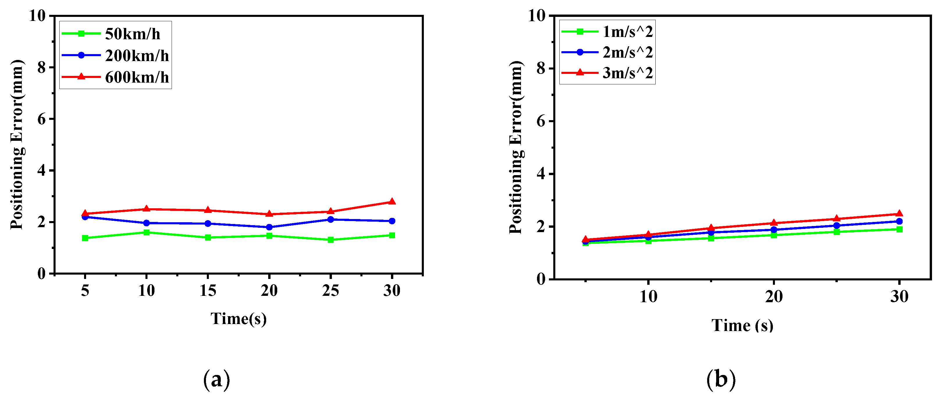
The positioning error during uniform and accelerated motion is shown in
Figure 16. It shows that the positioning error stabilizes at a constant millimetre level when the train speed is constant. Besides, when the train running speed increases, the positioning error increases slightly. This is because the positioning uses a combination of absolute and relative positions, and the position information is corrected each Gray-coded period. As a result, the accuracy of the position information can reach the millimetre level and the cumulative error is eliminated. The positioning error increases slightly when the running speed is too high, which is related to the processing speed of the simulator and the sampling rate of the GSPU.
The speed measurement error during uniform and accelerated motion is shown in
Figure 17. It shows that the speed measurement error is related to the running speed of the train. The faster the speed, the larger the absolute error error of speed measurement. However, from the point of view of relative error, when the running speed is 50 km/h, the relative error of speed measurement is about 2.14%. When the running speed is 600 km/h, the relative error of speed measurement is about 1.06%. When the train is running steadily, the fluctuation of the speed measurement error is also very small. This is also related to the speed measurement method, in which the GSPU is obtained by calculating the ratio of the distance
Δd between two adjacent crossing nodes of the loop and the elapsed time
Δt. This method effectively ensures the accuracy of speed measurement at low speeds. At the same time, when the speed increases, the elapsed time between adjacent intersections becomes shorter, and the absolute error of the speed measurement increases slightly, but the relative error decreases, which is in line with the expectation.
Table 4 shows the average error in positioning and speed measurement at low, medium and high speeds for 20 runs. Even in the high speed condition, the positioning error is only 2.58 mm, and the speed error is 6.34 km/h. The results show that the HIL platform can effectively simulate the various operation modes of high-speed maglev trains, and provides a reliable test environment for the GSPU. And the experiment also verifies the reliability and integrity of the GSPU function.
6. Discussion
In this paper, an HIL simulation platform based on the induction loops is built to solve the verification problem at the early stage of MPSS development. Firstly, a positioning method combining absolute position and relative position is proposed, and the principles of the two position detection methods are explained. The calculation process of key signals in MPSS is analyzed, and a simulation strategy based on parallel signal reconstruction is adopted. Based on this, the HIL simulation platform is built for GSPU, which is the core of MPSS. Finally, experimental validation of GSPU is carried out on this platform. The experimental results show that the HIL simulation platform is effective. It can accurately verify the positioning and speed measurement function of GSPU in various operation modes of high-speed maglev trains. Meanwhile, under the high-speed condition of 600 km/h, the positioning error of GSPU is only 2.58 mm, and the speed measurement error is 6.34 km/h. It validates the effectiveness of the positioning and velocity measurement method proposed in this paper.
Since the Gray-coded loops are inducing voltage signals through electromagnetic fields, then it is inevitably exposed to electromagnetic interference environment. To address this, GSPU has taken effective measures at both hardware and software levels. For example, the current frequency of the transmitting antenna is much higher than that of the traction motor, filtering is performed at the hardware level, and particle filtering algorithms are used at the software level. In addition, in order to expand the potential of the platform and adapt to a variety of operating modes, the train position algorithm of the HIL platform will be optimized in the future. By introducing the real speed curve when the maglev train is running, the whole operation mode of the train can be set flexibly to realize the simulation of different operation scenarios. What's more, the expansion interface is reserved in the platform, which provides the possibility of integrating the multi-train collaborative test as well as verifying the anti-interference performance of the GSPU in the future. It lays a solid foundation for subsequent research and diversification of applications. For the functional testing of other parts of the MPSS such as the transmitting antenna, it is recommended to build a motion simulation platform to carry out.
Author Contributions
Conceptualization, Cong Luo; Methodology, Linzi Yin, Cong Luo and Junfeng Cui; Software, Junfeng Cui; Validation, Cong Luo; Formal analysis, Cong Luo; Resources, Ling Liu; Data curation, Cong Luo; Writing – original draft, Linzi Yin; Writing – review & editing, Linzi Yin, Cong Luo, Ling Liu and Guoying Sun; Visualization, Junfeng Cui; Supervision, Linzi Yin, Ling Liu, Zhiming Liu and Guoying Sun; Project administration, Zhiming Liu; Funding acquisition, Guoying Sun.
Funding
This research was funded by Provincial Natural Science Foundation of Hunan: 2021JJ30877.
Institutional Review Board Statement
Not applicable.
Informed Consent Statement
Not applicable.
Data Availability Statement
The raw data supporting the conclusions of this article will be made available by the authors on request.
Acknowledgments
We thank CRSC Research & Design Institute Group Co., Ltd. for providing the experimental environment and experimental materials for this paper. The technical support for our research is also included.
Conflicts of Interest
Authors Cong Luo, Ling Liu, Junfeng Cui, Zhiming Liu and Guoying Sun were employed by CRSC Research & Design Institute Group Co.,Ltd. The remaining authors declare that the research was conducted in the absence of any commercial or financial relationships that could be construed as a potential conflict of interest.
Abbreviations
The following abbreviations are used in this article:
| MPSS |
Maglev Positioning and Speed measurement System |
| HIL |
Hardware-In-the-Loop |
| FPGA |
Field Programmable Gate Array |
| GSPU |
Ground Signal Processing Unit |
| TCS |
Traction Control System |
| EMI |
ElectroMagnetic Interference |
| LIM |
Linear Induction Motors |
| OCS |
Operation Control Systems |
| PWM |
Pulse Width Modulation |
| VTU |
Vehicle Transmission Unit |
| ILU |
Induction Loop Unit |
References
- Yan, L. Development and Application of the Maglev Transportation System. IEEE Transactions on Applied Superconductivity 2008, 18, 92–99. [CrossRef]
- Lin, P.; Deng, Z.; Ke, Z.; Lei, W.; Wang, X.; Ren, K. Dynamic Characteristics and Working Modes of Permanent Magnet Electrodynamic Suspension Vehicle System Based on Six Wheels of Annular Halbach Structure. Technologies 2023, 11, 16–16. [CrossRef]
- Ding, J.; Yang, X.; Long, Z.; Dang, N. Three-Dimensional Numerical Analysis and Optimization of Electromagnetic Suspension System for 200 Km/H Maglev Train Considering Eddy Current Effect. IEEE Access 2018, 6, 61547–61555. [CrossRef]
- Zhu, Q.; Wang, S.; Ni, Y. A Review of Levitation Control Methods for Low- and Medium-Speed Maglev Systems. Buildings 2024, 14, 837–837. [CrossRef]
- Zhang, D.; Long, Z.; Dai, C. Design and Realization of a Novel Position-And-Speed Measurement System with Communication Function for the Low-Speed Maglev Train. Sensors and Actuators A Physical 2013, 203, 261–271. [CrossRef]
- Jiang, S.; Wang, Y.; Liang, L.; Zhang, H.; Deng, Z. Truth-Correction-Based Multisensor Fusion Method for HTS Maglev Train’s Position Detection. IEEE Transactions on Instrumentation and Measurement 2023, 73, 1–14. [CrossRef]
- Li, F.; Sun, Y.; Xu, J.; He, Z.; Lin, G. Control Methods for Levitation System of EMS-Type Maglev Vehicles: An Overview. Energies 2023, 16, 2995–2995. [CrossRef]
- Xu, Y.; Fan, K.; Hu, Q.; Zhang, X. Positioning of Suspended Permanent Magnet Maglev Trains Using Satellite-Ground Multi-Sensor Fusion. IEEE Sensors Journal 2024, 24, 16816–16825. [CrossRef]
- Huang, W.; Tong, X.; Zeng, F.; Li, C.; Wang, Y. Maglev Train High-Precision Positioning Technology Based on FBG Array Time Division Multiplexing. Measurement 2024, 115160–115160. [CrossRef]
- Zhang, L.; Huang, J. Dynamic Interaction Analysis of the High-Speed Maglev Vehicle/Guideway System Based on a Field Measurement and Model Updating Method. Engineering Structures 2019, 180, 1–17. [CrossRef]
- Mihalič, F.; Truntič, M.; Hren, A. Hardware-In-The-Loop Simulations: A Historical Overview of Engineering Challenges. Electronics 2022, 11, 2462. [CrossRef]
- Montoya, J.; Brandl, R.; Vishwanath, K.; Johnson, J.; Darbali-Zamora, R.; Summers, A.; Hashimoto, J.; Kikusato, H.; Ustun, T.S. Advanced Laboratory Testing Methods Using Real-Time Simulation and Hardware-In-The-Loop Techniques: A Survey of Smart Grid International Research Facility Network Activities. Energies 2020, 13, 3267. [CrossRef]
- Arzate-Rivas, O.; Víctor Sámano-Ortega; Martínez-Nolasco, J.; Santoyo-Mora, M.; Martínez-Nolasco, C.; León-Lomelí, R.D. IoT Energy Management System Based on a Wireless Sensor/Actuator Network. Technologies 2024, 12, 140–140. [CrossRef]
- Amel Kasri; Kamel Ouari; Youcef Belkhier; Adel Oubelaid; Bajaj, M.; Milkias Berhanu Tuka Real-Time and Hardware in the Loop Validation of Electric Vehicle Performance: Robust Nonlinear Predictive Speed and Currents Control Based on Space Vector Modulation for PMSM. Results in Engineering 2024, 22, 102223–102223. [CrossRef]
- Wei, B. Discussion on Test Scheme for Train Integrity Functions in New Train Control System. Railway Signalling & Communication Engineering 2023, 20(05), 21-26+31. [CrossRef]
- Sun, X.; Jin, Z.; Xue, M.; Tian, X. Adaptive ECMS with Gear Shift Control by Grey Wolf Optimization Algorithm and Neural Network for Plug-in Hybrid Electric Buses. IEEE transactions on industrial electronics 2024, 71, 667–677. [CrossRef]
- Marinescu, A.; Taylor, A.; Clarke, S.; Serban, I.; Marinescu, C. Optimising Residential Electric Vehicle Charging under Renewable Energy: Multi-Agent Learning in Software Simulation and Hardware-In-The-Loop Evaluation. International Journal of Energy Research 2019, 43, 3853–3868. [CrossRef]
- Yang, X.; Yang, C.; Peng, T.; Chen, Z.; Liu, B.; Gui, W. Hardware-In-The-Loop Fault Injection for Traction Control System. IEEE Journal of Emerging and Selected Topics in Power Electronics 2018, 6, 696–706. [CrossRef]
- Zhao, Y.; Liu, Y.; Yang, S.; Liao, Y.; Chen, Z. Analysis on New Semi-Active Control Strategies to Reduce Lateral Vibrations of High-Speed Trains by Simulation and Hardware-In-The-Loop Testing. Proceedings of the Institution of Mechanical Engineers, Journal of Rail and Rapid Transit 2022, 236, 960–972. [CrossRef]
- Bernal, E.; Maksym Spiryagin; Cole, C. Ultra-Low Power Sensor Node for On-Board Railway Wagon Monitoring. IEEE Sensors Journal 2020, 20, 15185–15192. [CrossRef]
- Hägele, N.; Dignath, F. Vertical Dynamics of the Maglev Vehicle Transrapid. Multibody System Dynamics 2008, 21, 213–231. [CrossRef]
- Wang, H.; Ge, X.; Liu, Y.-C. Second-Order Sliding-Mode MRAS Observer-Based Sensorless Vector Control of Linear Induction Motor Drives for Medium-Low Speed Maglev Applications. IEEE Transactions on Industrial Electronics 2018, 65, 9938–9952. [CrossRef]
- Hu, H.; Zhong, J.; Chen, Y.; Ge, Q.; Wang, T. Research on Sectional Constant Slip Control of Linear Induction Motor Based on Parameter Self-Tuning. Energy Reports 2023, 9, 979–989. [CrossRef]
- Behzad Jandaghi; Venkata Dinavahi Hardware-In-The-Loop Emulation of Linear Induction Motor Drive for MagLev Application. IEEE Transactions on Plasma Science 2016, 44, 679–686. [CrossRef]
- Zhang, W.; Lin, G.; Hu, K.; Liao, Z.; Wang, H. Operation Control Method for High-Speed Maglev Based on Fractional-Order Sliding Mode Adaptive and Diagonal Recurrent Neural Network. Energies 2023, 16, 4566–4566. [CrossRef]
- Cao, X.; Ge, Q.; Zhu, J.; Kong, G.; Zhang, B.; Wang, X. Improved Sliding Mode Traction Control Combined Sliding Mode Disturbance Observer Strategy for High-Speed Maglev Train. IEEE Transactions on Power Electronics 2023, 38, 827–838. [CrossRef]
- Yang, J.; Gao, T.; Yuan, S.; Shi, H.; Zhang, Z. Research on Hardware-In-The-Loop Simulation of Single Point Suspension System Based on Fuzzy PID. International Journal of Grid and Utility Computing 2020, 11, 291–291. [CrossRef]
- Onur Akbatı; Hatice Didem Üzgün; Akkaya, S. Hardware-In-The-Loop Simulation and Implementation of a Fuzzy Logic Controller with FPGA: Case Study of a Magnetic Levitation System. Transactions of the Institute of Measurement and Control 2018, 41, 2150–2159. [CrossRef]
- Cao, X.; Ge, Q.; Zhu, J.; Zhao, L.; Zeng, D. Periodic Traction Force Fluctuations Suppression Strategy of Maglev Train Based on Flux Linkage Observation and Harmonic Current Injection. IEEE Transactions on Transportation Electrification 2023, 9, 3434–3451. [CrossRef]
- Zhu, J.; Cao, X.; Ge, Q.; Zeng, D. Adaptive-SMO-Based Traction Force Fluctuation Suppression Strategy Considering Suspension System for High-Speed Maglev Train. IEEE Transactions on Industrial Electronics 2024, 71, 2289–2299. [CrossRef]
- Lee, H.-W.; Kim, K.-C.; Lee, J. Review of Maglev Train Technologies. IEEE Transactions on Magnetics 2006, 42, 1917–1925. [CrossRef]
- Zhong, Z.; Shao, Z.; Yang, M.; Wang, X.; Xiao, Q.; Wang, Y. Quasi-Synchronous Operation Principle of a Variable Air-Gap Doubly Fed Linear Motor for High-Speed Maglev Application. IEEE Transactions on Transportation Electrification 2023, 9, 2929–2940. [CrossRef]
- Sun, L.; Taylor, J.; Guo, X.; Cheng, M.; Emadi, A. A Linear Position Measurement Scheme for Long-Distance and High-Speed Applications. IEEE Transactions on Industrial Electronics 2020, 68, 4435–4447. [CrossRef]
- Jo, J.-M.; Lee, J.-H.; Han, Y.-J.; Lee, C.-Y.; Lee, K.-S. Development of Propulsion Inverter Control System for High-Speed Maglev Based on Long Stator Linear Synchronous Motor. Energies 2017, 10, 170–170. [CrossRef]
- Dai, C.; Dou, F.; Song, X.; Long, Z. Analysis and Design of a Speed and Position System for Maglev Vehicles. sensors 2012, 12, 8526–8543. [CrossRef]
- Jo, J.-M.; Lee, C.-Y.; Kim, J.H. Relationship between the Shape of Cross-Inductive Loop Coils and the Induced Voltage for Position Detection System. Electronics Letter 2024, 60. [CrossRef]
- Dou, F.; Dai, C.; Xie, Y. Filtering Algorithm and Direction Identification in Relative Position Estimation Based on Induction Loop-Cable. Journal of Central South University 2016, 23, 112–121. [CrossRef]
Figure 1.
Block diagram of MPSS .
Figure 1.
Block diagram of MPSS .
Figure 2.
Address loops coding method. Half the distance between two adjacent crossing nodes of a G0 loop is the Gray coding period.
Figure 2.
Address loops coding method. Half the distance between two adjacent crossing nodes of a G0 loop is the Gray coding period.
Figure 3.
Principle of relative position detection.
Figure 3.
Principle of relative position detection.
Figure 4.
G0 and SG0 loop signals.
Figure 4.
G0 and SG0 loop signals.
Figure 5.
The magnetic flux in the induction loop circuit.
Figure 5.
The magnetic flux in the induction loop circuit.
Figure 6.
Magnetic induction inside the loop.
Figure 6.
Magnetic induction inside the loop.
Figure 7.
Transmitting antenna model.
Figure 7.
Transmitting antenna model.
Figure 8.
Structure of the HIL simulation platform.
Figure 8.
Structure of the HIL simulation platform.
Figure 9.
Operation of the simulation system.
Figure 9.
Operation of the simulation system.
Figure 10.
(a) It shows the physical GSPU, emulator and host computer; (b) It shows the eight groups of induction loops and the corresponding eight transmitting antennas of the HIL simulation platform.
Figure 10.
(a) It shows the physical GSPU, emulator and host computer; (b) It shows the eight groups of induction loops and the corresponding eight transmitting antennas of the HIL simulation platform.
Figure 11.
Absolute position Gray code processing results.
Figure 11.
Absolute position Gray code processing results.
Figure 12.
G0 and SG0 loop signals processing results.
Figure 12.
G0 and SG0 loop signals processing results.
Figure 13.
Relative position processing results. It is expressed in angular form and its value varies between 0 and 360.
Figure 13.
Relative position processing results. It is expressed in angular form and its value varies between 0 and 360.
Figure 14.
Instantaneous position processing results.
Figure 14.
Instantaneous position processing results.
Figure 15.
Accelerated mode absolute position processing results.
Figure 15.
Accelerated mode absolute position processing results.
Figure 16.
(a) It shows the positioning error during uniform motion at different speeds; (b) It shows the positioning error during accelerated motion at different accelerations.
Figure 16.
(a) It shows the positioning error during uniform motion at different speeds; (b) It shows the positioning error during accelerated motion at different accelerations.
Figure 17.
(a) It shows the speed measurement error during uniform motion at different speeds; (b) It shows the speed measurement error during accelerated motion at different accelerations.
Figure 17.
(a) It shows the speed measurement error during uniform motion at different speeds; (b) It shows the speed measurement error during accelerated motion at different accelerations.
Table 1.
Comparative analysis of the proposed HIL simulation platform and existing solutions.
Table 1.
Comparative analysis of the proposed HIL simulation platform and existing solutions.
| Solution |
Test Object |
Cost |
Complexity |
Ease of Implementation |
Accuracy |
Flexibility |
| Traditional Hardware-based1
|
actual requirements |
high |
high |
low |
low |
low |
| Existing HIL-based2 |
LIM |
low |
high |
low |
high |
low |
| OCS |
moderate |
high |
moderate |
moderate |
low |
| TCS |
moderate |
low |
low |
high |
low |
| Proposed HIL Platform |
MPSS |
low |
low |
high |
high |
high |
Table 2.
Parameters set by the HIL simulation platform. Physical parameters and parameters for train operation in three modes are included.
Table 2.
Parameters set by the HIL simulation platform. Physical parameters and parameters for train operation in three modes are included.
| Parameter Item |
Parameter Setting |
| physical parameters |
transmitting antennas |
|
| induction loops |
|
| operating parameters |
instantaneous speed mode |
|
| instantaneous position mode |
|
| acceleration mode |
|
Table 3.
Parameters set by the HIL simulation platform. Physical parameters and parameters for train operation in three modes are included.
Table 3.
Parameters set by the HIL simulation platform. Physical parameters and parameters for train operation in three modes are included.
| Software Modules |
LUT |
Flip-Flop |
Block RAM |
| Analogue position calculation |
1.19% |
0.08% |
0.41% |
| Calculation of PWM parameters |
1.48% |
0.21% |
0.58% |
| PWM signal generation |
0.43% |
0.15% |
0.78% |
| Communication |
3.73% |
1.73% |
1.38% |
| Totals |
6.83% |
2.17% |
3.15% |
Table 4.
Positioning and speed measurement errors.
Table 4.
Positioning and speed measurement errors.
| Speed |
Average Error |
| Positioning(mm) |
Speed Measurement(km/h) |
| 50 km/h |
1.47 |
1.07 |
| 200 km/h |
1.92 |
3.19 |
| 600 km/h |
2.58 |
6.34 |
|
Disclaimer/Publisher’s Note: The statements, opinions and data contained in all publications are solely those of the individual author(s) and contributor(s) and not of MDPI and/or the editor(s). MDPI and/or the editor(s) disclaim responsibility for any injury to people or property resulting from any ideas, methods, instructions or products referred to in the content. |
© 2025 by the authors. Licensee MDPI, Basel, Switzerland. This article is an open access article distributed under the terms and conditions of the Creative Commons Attribution (CC BY) license (http://creativecommons.org/licenses/by/4.0/).