
Submitted:
04 March 2025
Posted:
05 March 2025
You are already at the latest version
Abstract
This study evaluates the ICESat-2 ATL13 altimetry product for water level estimation in 182 Canadian lakes by integrating satellite-derived observations with in situ measurements and applying spatial filtering based on the HydroLAKES dataset. Statistical metrics, including root mean square error (RMSE), mean absolute error (MAE), and mean bias error (MBE), were employed to quantify the discrepancies between datasets. Notably, the application of HydroLAKES filtering reduced the mean RMSE from 1.53 m to 1.40 m, and further exclusion of high-error cases lowered the RMSE to 0.96 m. Larger, deeper lakes exhibited lower error margins, whereas smaller lakes with complex shorelines were more prone to variability. Regression analysis confirmed an excellent correspondence between satellite and gauge measurements (R² = 0.9999; Pearson’s r = 0.9999, p < 0.0001). Temporal analysis revealed water level declines in 134 lakes and increases in 48 lakes, suggesting potential influences of climatic variability and anthropogenic activity. These findings underscore the promise of integrating ICESat-2 altimetry with HydroLAKES-based filtering for robust inland water monitoring, while also highlighting the need for further refinement in data-processing algorithms and site-specific calibration.
Keywords:
ICESat-2
; Canadian lakes
; altimetry
; HydroLAKES
1. Introduction
Monitoring inland water levels with precision is crucial for understanding hydrological processes, managing water resources, and evaluating how climate change affects freshwater systems [1]. Lakes, as natural reservoirs, play a key role in regulating the water cycle, shaping regional climate patterns, and sustaining diverse ecosystems [2]. They also serve as essential resources for human activities, including agriculture, hydroelectric power generation, and drinking water supply. However, lake and river water levels fluctuate over time and space due to various factors such as precipitation, evaporation, groundwater interactions, and human interventions like dam operations and water extraction [3]. Understanding these variations is vital for mitigating environmental risks and ensuring sustainable water management. As climate variability increases, the demand for precise, continuous, and wide-ranging water level data has never been greater, highlighting the limitations of traditional hydrological monitoring methods [4].
Traditionally, water levels have been monitored using in situ gauge stations, which offer highly accurate and continuous observations over time. While these ground-based measurements are invaluable for local and regional hydrological assessments, their spatial coverage is inherently limited [5]. Most monitoring networks are concentrated in accessible or economically significant regions, leaving vast and often remote areas with little to no coverage. This issue is particularly pronounced in high-latitude or sparsely populated regions, where logistical and financial challenges make it difficult to install and maintain gauge stations. As a result, critical data gaps persist, limiting our ability to develop comprehensive hydrological models and respond effectively to environmental changes [6]. The restricted spatial reach of gauge-based networks has driven the search for alternative measurement techniques capable of providing extensive and consistent observations across large areas [7].
In recent decades, satellite altimetry has revolutionized hydrological monitoring by providing extensive spatial coverage and enabling the global observation of inland water bodies. Unlike traditional gauge stations, satellite-based measurements are not constrained by accessibility and can offer consistent water level data across vast and remote regions [8]. Early radar altimetry missions, such as TOPEX/Poseidon, Jason-1/2/3, and ENVISAT, demonstrated that spaceborne sensors could estimate water levels by measuring the time delay of radar pulses reflected from water surfaces [9,10,11]. However, these missions were primarily designed for open-ocean observations and had relatively coarse spatial resolutions, making them less effective for monitoring smaller lakes and rivers [12]. A major step forward in inland water monitoring came with NASA’s Ice, Cloud, and Land Elevation Satellite (ICESat) mission, launched in 2003. As the first spaceborne lidar altimeter dedicated to precise elevation measurements, ICESat provided valuable insights into ice sheet dynamics, land topography, and inland water levels [13]. However, its single-beam laser system and intermittent data acquisition posed limitations in spatial and temporal coverage [14,15]. Building upon its predecessor’s legacy, the launch of ICESat-2 in 2018 marked a significant technological advancement. Equipped with the Advanced Topographic Laser Altimeter System (ATLAS), ICESat-2 employs a photon-counting lidar system that delivers high-resolution elevation measurements with sub-decimeter accuracy [16]. By using multiple laser beams, ICESat-2 significantly improves spatial coverage and data density, enabling the precise monitoring of even narrow and complex inland water bodies [10]. This advancement has opened new possibilities for tracking water level variations at unprecedented scales, further enhancing our ability to study hydrological processes and climate-driven changes in freshwater systems [17,18,19].
While ICESat-2 represents a significant advancement in satellite altimetry, challenges remain regarding the reliability and applicability of its ATL13 data product for water level estimation. Despite its high-resolution laser altimetry offering substantial improvements over traditional radar-based methods, various environmental factors can still affect measurement accuracy [20]. Ice cover, surface wave dynamics, vegetation interference, and atmospheric conditions may introduce uncertainties in water level retrievals, potentially limiting the precision of the dataset [21,22,23,24]. Additionally, while larger lakes benefit from denser beam returns and stronger signal quality, smaller lakes especially those with irregular shorelines or fluctuating water levels present greater challenges for accurate measurement [25]. These complexities highlight the need for rigorous validation of ICESat-2-derived water levels using ground-based gauge station data. Ensuring the reliability of satellite altimetry for hydrological applications requires a comprehensive assessment of measurement uncertainties and a robust comparison with in situ observations to refine data processing techniques and enhance overall accuracy.
To address these challenges and enhance the accuracy of satellite-based water level monitoring, the integration of high-resolution geospatial datasets has proven to be essential. In this study, I leverage the HydroLAKES database, which provides detailed shoreline polygons for over 1.4 million lakes worldwide [26]. By defining precise lake boundaries, HydroLAKES allows for the spatial filtering of ATL13 measurements, reducing contamination from surrounding land surfaces and ensuring that only valid water surface returns are analyzed. This refinement is particularly crucial in cases where ICESat-2’s laser footprint overlaps with non-water areas, such as shorelines or adjacent land, which could introduce errors in water level estimation. By improving the spatial attribution of ICESat-2 data, HydroLAKES enhances the reliability of satellite-derived measurements and supports a more accurate representation of hydrological variability. This integration is especially valuable for smaller or irregularly shaped lakes, where precise delineation plays a key role in minimizing uncertainties and strengthening the overall robustness of satellite altimetry for inland water monitoring. Given that this study includes a significant number of small lakes, ensuring accurate boundary delineation is particularly important for capturing reliable water level estimates and reducing measurement errors in these challenging environments.
While satellite altimetry has made significant strides in hydrological monitoring, key research gaps persist, particularly in diverse and under-monitored aquatic environments. Most previous studies have focused on large, well-instrumented water bodies, where the availability of in situ data facilitates straightforward validation of satellite-derived measurements [27,28]. In contrast, many lakes, especially those in remote or high-latitude regions, lack dense gauge networks, making it challenging to assess the accuracy and applicability of satellite observations. Additionally, seasonal factors such as ice cover formation, snowmelt-driven runoff, and extreme precipitation events can introduce temporal variability that has not been systematically evaluated across different lake types [29]. This gap is particularly evident in Canada, which hosts an immense variety of lake ecosystems, ranging from glacially fed alpine lakes to extensive boreal and subarctic water bodies. Given Canada’s vast number of lakes, a comprehensive assessment of ICESat-2 ATL13 data across different lake sizes, morphologies, and climatic conditions is essential to determine the broader applicability of this remote sensing technology in hydrological studies. A key contribution of this study is the analysis of lakes across a wide range of latitudes, longitudes, elevations, depths, and surface areas, offering a more holistic evaluation of ICESat-2’s performance in varying hydrological and geographical contexts. By incorporating this diverse set of lakes, this research provides new insights into the robustness of satellite altimetry in capturing water level variations across different environmental settings, strengthening its integration with traditional hydrological monitoring methods.
This study provides a systematic evaluation of ICESat-2 ATL13 data for monitoring inland water levels across a diverse range of Canadian lakes. By integrating satellite altimetry with high-resolution geospatial datasets and in situ gauge measurements, we aim to assess the accuracy and applicability of remote sensing techniques in various hydrological settings. A key contribution of this work is the analysis of lakes spanning different latitudes, elevations, depths, and sizes, allowing for a comprehensive examination of environmental factors influencing ICESat-2 performance. The findings from this study will not only enhance the reliability of satellite-based water level estimation but also support the broader integration of remote sensing technologies into hydrological research and water resource management. As satellite altimetry continues to evolve, such efforts are essential for improving monitoring capabilities in data-scarce regions and advancing our understanding of freshwater dynamics in a changing climate.
2. Materials and Methods
2.1. Geographical Scope of the Study
The study encompasses 182 lakes distributed across Canada, representing a diverse array of hydrological, ecological, and morphological characteristics. These lakes are located across various climatic zones, from the boreal north to temperate regions in the south, providing an ideal framework for evaluating ICESat-2 ATL13 altimetry data. As illustrated in Figure 1, the lakes in the dataset exhibit significant variation in size and depth, with larger circles indicating expansive surface areas. The geographical spread highlights the lakes’ broad range of altitudes, depths, and surface areas. Examples include Great Slave Lake, among the largest and deepest, with a surface area of 26,734 km² and a depth of 59 meters; Lake Winnipeg, another expansive lake, with a surface area of 23,923 km² and a relatively shallow depth of 11.9 meters; Harrison Lake, notable for its depth of 194 meters, representing one of the deepest lakes in the study; and Lake Minnewanka, located at a significant altitude of 1,469 meters above sea level. The elevation distribution, however, is widespread, reflecting the diversity in the dataset without being dominated by extreme cases.
Figure 2 depicts the relationship between lake elevation and average depth, revealing a more widespread elevation distribution rather than isolated outliers. While most lakes cluster at lower elevations with shallow depths, exceptions like Harrison Lake for its depth and Lake Minnewanka for its elevation illustrate the dataset’s range and variability, providing valuable data for satellite altimetry studies.
Figure 3 presents a geodetic distance matrix of the 20 largest lakes, illustrating spatial relationships. Cooler colors in the heatmap indicate closer proximities, such as the Manitoba-Winnipegosis pair, while warmer tones represent greater separations, such as between Great Slave-Melville and Lesser Slave-Melville. This visualization captures both regional clusters and more distant, isolated lakes, emphasizing the geographical diversity of the study.
The selection of these 182 lakes was guided by criteria aimed at representing a broad spectrum of characteristics. The dataset includes lakes of varying depths, elevations, and surface areas, ensuring spatial representation across Canada. Lakes with significant surface areas were prioritized for robust altimetry analysis. Additionally, the availability of historical water level and gauge data enabled trend assessments. This diverse dataset, incorporating key examples such as Great Slave and Winnipeg alongside unique cases like Harrison Lake and Lake Minnewanka, provides a comprehensive representation of Canada’s inland water systems.
2.2. Data
2.2.1. ICESat-2 ATL13
In this study, I utilized ICESat-2 ATL13, a dataset specifically designed for inland water level monitoring. ICESat-2, launched in 2018, is equipped with the Advanced Topographic Laser Altimeter System (ATLAS), which provides high-precision measurements using photon-counting lidar [16]. Compared to radar altimetry missions like CryoSat-2 and Sentinel-3, ICESat-2 enables more accurate water level retrieval without requiring extensive geophysical corrections. ATL13 is derived from ATL03 Global Geolocated Photon data and isolates water surface photons along the satellite’s track. It provides orthometric heights (EGM2008) and includes parameters such as surface slope, wave height, and subsurface attenuation. For this study, I downloaded ATL13 data (.h5 format) from NSIDC and processed it using Python. Noise filtering and spatial masks were applied to ensure that only valid water surface returns were used. This approach improved the reliability of the derived water levels, making them suitable for hydrological analysis in remote regions.
2.2.2. HydroLAKES
In this study, I utilized HydroLAKES to delineate lake boundaries and constrain ICESat-2 ATL13 water level measurements. HydroLAKES provides high-resolution shoreline polygons for 1.4 million lakes worldwide with a surface area of at least 10 hectares [26]. The dataset integrates multiple sources and is co-registered with the HydroSHEDS global river network via lake pour points. HydroLAKES includes essential geometric attributes such as surface area, shoreline length, and estimated depth and volume, making it a valuable tool for hydrological research. By applying HydroLAKES as a spatial mask, I ensured that ICESat-2 photon data were strictly confined within lake boundaries, reducing potential contamination from surrounding land and vegetation. This approach enhanced the reliability of water level retrievals, particularly for lakes in remote and data-scarce regions.
2.2.3. Gauge Station Data
In this study, I utilized hydrometric gauge station data from the Water Survey of Canada (WSC) to validate and complement satellite-derived water level measurements. The WSC, in collaboration with provincial and territorial agencies, operates over 2,800 active hydrometric stations across Canada, monitoring water level, discharge, and sediment transport. Historical and real-time hydrometric data were obtained from HYDAT [30], the national archival database of the National Hydrometric Program. HYDAT contains records from over 2,500 active and 5,500 discontinued stations, providing long-term datasets essential for hydrological analysis. By integrating in situ gauge data with ICESat-2 ATL13 water levels, I ensured accurate validation of satellite observations. This approach enhances the reliability of water level estimates, particularly in calibrating remote sensing data for hydrological applications.
2.3. Methodology
This study follows a structured approach to extract and validate water levels from ICESat-2 ATL13 data. The workflow consists of data preprocessing and lake selection, outlier removal, water level extraction, and statistical analysis. HydroLAKES polygons and gauge station data are used for filtering and validation, while statistical methods ensure data accuracy.
2.3.1. Data Preprocessing and Lake Selection
The ICESat-2 ATL13 dataset, provided in .h5 format, was downloaded and processed using Python libraries to extract relevant photon data. To ensure that only water surface photons were retained, a spatial filtering approach was applied using HydroLAKES polygons. Each ICESat-2 photon was compared against HydroLAKES shoreline polygons, and only those falling within the defined lake boundaries were retained. This step eliminated photon returns from areas that contained water signals but were not classified as lakes in the HydroLAKES database, ensuring that only validated lake surfaces were considered.
A lake was considered eligible for inclusion in the analysis only if it met a set of specific criteria designed to ensure the reliability, consistency, and scientific validity of the data used in this study.
- Presence of a Gauge Station: To facilitate validation, a hydrometric gauge station had to be associated with the lake. Each station location was cross-referenced with HydroLAKES polygons, and only lakes with corresponding in situ measurements were selected.
- Inclusion in HydroLAKES: Only lakes identified in HydroLAKES (≥ 10 ha surface area) were considered to ensure data consistency and compatibility with established lake classifications.
- Sufficient ICESat-2 Observations: The lake needed to have at least 10 days of ICESat-2 ATL13 measurements to enable a meaningful temporal analysis.
Additionally, to ensure compatibility between satellite and gauge station data, temporal alignment was verified. Some hydrometric stations had ceased data collection before the ICESat-2 mission launch in 2018, making their records unsuitable for validation. Therefore, only lakes with overlapping ICESat-2 and gauge station observation periods were retained for analysis.
2.3.2. Outliers Removal
In ATL13 water level measurements, extreme or unexpected values can occasionally occur due to sensor errors, transient atmospheric effects, or other data collection conditions. These outliers can negatively impact both the accuracy and reliability of subsequent analyses, making a systematic approach to outlier detection and removal essential. In my research, I adopt the Interquartile Range (IQR) method for identifying and filtering outlier points, primarily because it is robust, easy to implement, and well-suited to data exhibiting a generally mild skew.
The IQR approach focuses on the middle 50% of the data, relying on the first quartile Q1 (the 25th percentile) and the third quartile Q3 (the 75th percentile). Mathematically, the interquartile range is defined in Equation (1):
Observations that fall outside the interval shown in Equation (2) are flagged as potential outliers:
where k is often set to 1.5 but can be increased up to 3 to be more conservative and reduce the risk of removing valid rare observations. In this study, I tested several values of k (1.5, 2, 2.5, and 3) to find the optimal threshold for the ATL13 data. The results indicated that k=2 provides the best balance between filtering out erroneous measurements and preserving valid ones, so I used k=2 in all subsequent analyses.
I chose the IQR method for several reasons. First, it relies on percentiles and is therefore less affected by outliers than methods based on the mean and standard deviation. This makes it more robust to skewed distributions and occasional extreme measurements, which often appear in water level data. Second, the distribution of ATL13 measurements commonly approximates a normal or mildly skewed shape, so the middle 50% of the data (from Q1 to Q3) adequately represents the typical variation. Third, calculating quartiles and determining the IQR is computationally straightforward, even for large datasets, and the resulting threshold range is easy to visualize and interpret (for instance, via boxplots).
Practically, I gather the ATL13 water level readings into a single column, remove or flag null entries, compute Q1 and Q3, and then use Equations (1) and (2) with k=2 to determine which measurements should be deemed outliers. Although I label these points as outliers from a purely statistical perspective, I always investigate whether some of them might reflect genuine physical events—such as floods or sensor calibration shifts—rather than mere measurement errors. By employing the IQR method with k=2, I effectively filter out anomalous and implausible values, thereby improving both the reliability of subsequent analyses and the interpretability of the results. This outlier removal process is crucial for ensuring that the statistical conclusions drawn from the ATL13 data remain valid and trustworthy.
2.3.3. Water Level Extraction
To derive representative water levels from ICESat-2 ATL13 data, I adopted a method that evaluates both individual photon measurements and their aggregated values against reference gauge station readings. For each day, all valid photon returns were compared to the corresponding in situ gauge station data, ensuring temporal discrepancies were limited to a maximum of hourly differences. This alignment significantly improved the reliability of the analysis.
By calculating the difference between each photon measurement and the reference gauge reading, I conducted a statistical assessment of individual photon reliability. This allowed not only an evaluation of the accuracy and consistency of individual photon returns but also a determination of how well the daily mean or median water surface elevation aligned with the reference values. Additionally, comparisons and analyses were conducted based on diverse lake-specific criteria such as depth, surface area, elevation, and geographic location. This allowed the predictions to be further tailored to the unique characteristics of each lake, enhancing the robustness of the derived water levels. Aggregation strategies, including the use of the mean or median water surface elevation, were employed to mitigate noise and outliers in the data. Temporal averaging further enhanced the stability and reliability of the derived water levels. This multi-level evaluation ensured that both individual photon measurements and their aggregated values were robust, accurate, and consistent with reference readings, providing high confidence in the results.
2.3.4. Advanced Statistical Analysis: Refined Hydrological Assessment
A rigorous statistical assessment was conducted to evaluate the performance of ICESat-2-derived water level estimates by comparing them with in situ gauge measurements. This analysis incorporated a combination of error quantification, regression and correlation modeling, and error distribution assessments in both temporal and spatial contexts to ensure a comprehensive and reproducible evaluation. Table 1 summarizes the statistical techniques applied in this study, outlining the methodologies and key performance metrics used in the assessment.
To quantify the discrepancies between ICESat-2-derived water levels and in situ gauge measurements, standard error metrics such as Root Mean Square Error (RMSE), Mean Absolute Error (MAE), and Mean Bias Error (MBE) were employed. RMSE was used to measure the magnitude of differences, giving greater weight to larger deviations and providing an overall assessment of error severity. MAE, on the other hand, represented the average absolute differences between datasets, offering a straightforward measure of accuracy. MBE was calculated to determine whether the satellite-derived estimates systematically over- or underestimated gauge station measurements. The mathematical representations of these metrics are given as follows:
To further assess the relationship between ICESat-2-derived water levels and in situ gauge measurements, a linear regression model was applied. This model, expressed as
included an intercept term (β0), a slope coefficient (β1), and an error term (ϵi). The coefficient of determination (R2) was used to quantify the proportion of variance in the ICESat-2 estimates explained by gauge station measurements, providing insight into the model’s explanatory power. Additionally, Pearson’s correlation coefficient (r) was calculated to determine the strength of the linear association between the datasets. In cases where normality assumptions were not met, Spearman’s rank correlation (ρ) was used to assess the monotonic relationship between the variables. The formula for Pearson’s correlation coefficient is given by
To investigate the nature of residuals () both graphical and statistical methods were applied. The distribution of errors was visualized using histograms and Kernel Density Estimation (KDE) plots, while the Shapiro-Wilk test was performed to statistically assess normality. If significant deviations from normality were detected, non-parametric statistical techniques were employed to ensure robustness in the analysis.
Further, temporal and spatial stratification was carried out to analyze how errors varied under different conditions. Daily boxplots were generated to observe fluctuations over time, while lake-specific stratifications were performed based on surface area, depth, and geographic location. This stratified analysis helped identify region-specific trends that influenced the reliability of satellite-derived water level estimates, offering a more nuanced understanding of the data’s performance across diverse hydrological environments.
Since ICESat-2-derived water levels rely on photon-counting lidar, the density of photon returns plays a crucial role in determining measurement accuracy. To examine this effect, RMSE and MAE values were analyzed across different point densities, assessing whether increased photon density led to significant improvements in precision. The results of this analysis provided important insights into how variations in lidar point density influenced error magnitudes and contributed to enhancing the accuracy of satellite-based hydrological assessments.
By integrating multiple statistical techniques, this study ensures a rigorous, transparent, and reproducible evaluation of ICESat-2-derived water levels. The combined use of regression models, correlation coefficients, error distribution assessments, and stratified analyses provides a comprehensive framework for assessing satellite altimetry data in hydrological research. These findings not only validate the accuracy of satellite-derived measurements but also highlight specific factors that influence their reliability, ultimately guiding improvements in the use of satellite-based altimetry for water level monitoring.
3. Results and Discussions
3.1. Error Metrics Evaluation and Filtering Effects on ICESat-2 Water Level Estimates
ICESat-2 altimetry-derived water level estimates were evaluated by examining the Root Mean Square Error (RMSE), Mean Absolute Error (MAE), and Mean Bias Error (MBE) for both filtered and unfiltered datasets. As illustrated in Figure 4, filtering successfully reduces overall error magnitudes, although certain outliers remain, often clustered within a small subset of lakes. For instance, Hylak ID 8130, 2867, and 64 consistently exhibit larger errors in RMSE, MAE, and MBE, suggesting that the measurement inconsistencies may stem from site-specific hydrological or retrieval conditions rather than a broad, systematic bias.
Despite the persistence of these local anomalies, the filtering process substantially improves the overall accuracy of ICESat-2 measurements. When considering all lakes and all observation dates, the mean RMSE decreases from 1.53 m in the unfiltered data to 1.40 m in the filtered data. Excluding the few lakes that exhibit extreme errors reduces the mean RMSE from 1.27 m (unfiltered) to 0.96 m (filtered), demonstrating that a small group of problematic stations disproportionately elevates the overall error metrics. Similar improvements are evident in MAE and MBE, indicating both reduced overall error and diminished bias after filtering. The mean MBE of -0.6 m points to a systematic underestimation of water levels compared to in situ measurements, which may be influenced by factors such as lidar’s penetration at the water surface, suboptimal atmospheric corrections, or potential algorithmic biases.
Figure 5 focuses on the 20 largest lakes and highlights that for most of these water bodies, RMSE and MAE remain below 1.0 m, suggesting that ICESat-2 performs reliably over large, open-water systems. However, Lake Winnipeg and Wollaston Lake show noticeably higher error levels for both RMSE and MAE, implying that local conditions—such as complex shorelines or other hydrodynamic processes—could introduce additional uncertainties. Examining MBE across these large lakes reveals that most do not exhibit a strong bias, yet Lake Winnipeg tends to be positively biased (overestimation), while Wollaston Lake is negatively biased (underestimation). This divergence underscores the potential need for site-specific calibration or additional correction procedures that account for distinctive lake characteristics.
Overall, the results presented in Figure 4 and Figure 5 emphasize that data filtering substantially enhances the accuracy of ICESat-2 water level estimations while exposing certain lakes that demand closer inspection due to unusually high error values. The fact that most large lakes exhibit relatively low RMSE and MAE demonstrates the broad applicability of ICESat-2 altimetric measurements, yet the outlier lakes highlight how local influences can amplify measurement errors. These findings ultimately suggest that selective filtering coupled with targeted calibration strategies may further refine the accuracy of satellite-derived water levels, particularly in hydrologically or morphologically complex environments.
3.2. Regression and Correlation Analysis
ICESat-2-derived water levels were compared against in situ gauge measurements through both regression and correlation analyses applied to unfiltered and filtered datasets. As illustrated in Figure 6, the results demonstrate a near-perfect alignment between satellite estimates and gauge observations, underscoring the high reliability of ICESat-2 altimetry for water level retrieval.
In the linear regression models, the coefficient of determination (R²) reached an exceptionally high value of 0.9999 for both datasets, indicating that nearly all of the variance in the ICESat-2 data is explained by gauge measurements. Moreover, the regression slopes remain close to unity in both unfiltered and filtered scenarios, suggesting a near 1:1 relationship between the two measurement sources. For the unfiltered dataset, the slope is 1.0001 with an intercept of 0.0104 m, whereas the filtered dataset yields a slope of 0.9999 and an intercept of 0.0650 m—both indicative of negligible deviations from a perfect fit. These findings confirm the consistency of ICESat-2 measurements with gauge records, while also revealing that filtering introduces only minor adjustments to the absolute water level values.
Correlation metrics further support the robustness of ICESat-2 altimetry. Pearson’s correlation coefficient (r) stands at 0.9999 (p < 0.0001) for both datasets, signifying an almost perfect linear relationship, and Spearman’s rank correlation coefficient (ρ)—which assesses the monotonic order of the observations—improves from 0.9790 to 0.9831 after filtering. This increase indicates that data filtering reduces local anomalies and refines the overall data consistency without compromising the core integrity of the ICESat-2 measurements.
Collectively, these results affirm that ICESat-2 altimetry provides highly accurate water level estimates in strong agreement with in situ gauges. While the filtering process subtly influences intercept values, its practical impact on hydrological assessments remains minimal. The enhanced Spearman correlation further demonstrates the merit of targeted filtering in managing localized errors, highlighting the value of such refinements for improving data reliability in diverse aquatic environments.
3.3. Error Distribution Characteristics
Residuals from the regression analyses were examined using the Shapiro–Wilk and Kolmogorov–Smirnov tests, alongside histogram, Kernel Density Estimation (KDE), and Q–Q plot evaluations. These procedures were conducted on both unfiltered and filtered datasets, and the combined findings are presented in Figure 7.
Statistical tests (Shapiro–Wilk and Kolmogorov–Smirnov) returned p-values of 0.0000 for both unfiltered and filtered datasets, suggesting that residuals in neither dataset strictly follow a normal distribution. In the histogram and KDE plots, unfiltered residuals appear more dispersed, featuring heavier tails and a greater presence of outliers. By contrast, filtering reduces these extreme values, resulting in a narrower, more concentrated distribution, though some skewness remains. Q–Q plots reinforce these observations. While the bulk of points in the filtered dataset align reasonably well with the theoretical normal line, a number of data points still deviate in the tails, reflecting persistent departures from ideal normality. Notably, these outliers often correspond to the same lakes identified in earlier sections, where highly irregular shorelines and potentially unrepresentative gauge stations may introduce additional variability. Although these deviations indicate that standard assumptions of linear regression may not be perfectly met, the overall performance of the ICESat-2 water level estimates remains robust, particularly for the majority of lakes where residuals are relatively well-behaved. In instances where coastline complexity or other site-specific factors play a larger role, further refinements such as data transformations, robust regression methods, or site-specific calibrations could help refine residual distributions without detracting from the broader reliability of the approach.
In summary, while the residuals are not strictly normal in either dataset, the filtering process markedly reduces outliers, bringing most data points closer to a normal-like distribution. The persistent deviations observed largely arise from a small subset of lakes with intricate shoreline morphologies. Recognizing and accounting for these localized conditions can enhance model performance and ensure that the strong agreement between ICESat-2 and gauge-derived water levels extends across a range of hydrological settings.
3.4. Spatial Variability of Errors
In order to explore how various hydrological characteristics may influence the accuracy of ICESat-2-derived water levels, RMSE was examined in relation to lake area, depth, and elevation. Figure 8 presents these three relationships with red regression lines highlighting overall trends. The log-scaled plot of lake area reveals that larger lakes tend to exhibit lower and more stable RMSE values, while smaller lakes display substantial variation, including a few extreme error cases. Although there is a slight upward trend in the regression curve, considerable uncertainty remains for very large lakes, suggesting that other local factors may also affect these errors. One plausible explanation is that ICESat-2’s measurement footprint may capture limited coverage in smaller lakes, making edge effects more pronounced and thus increasing errors. In contrast, larger lakes benefit from a broader range of satellite observations, effectively smoothing out local anomalies and reducing overall RMSE.
Further analysis of RMSE values in the context of average lake depth indicates that shallow lakes (particularly those with depths of 0–30 m) are prone to greater measurement variability. Elevated surface disturbance, turbidity, and other near-surface processes in these shallow environments could explain the higher error magnitudes. Although deeper lakes typically yield more consistent, lower RMSE, outliers persist in certain cases, implying that localized conditions—such as complex bathymetry or specific environmental factors—may affect measurement precision. The regression line suggests a modest upward trend in RMSE as depth increases, but the widespread distribution of data points complicates conclusive interpretations.
When examining elevation, the data indicate that lower-lying lakes generally show wider variations in RMSE, whereas higher-elevation lakes tend to have fewer errors. The negative slope in the regression line aligns with a potential reduction in environmental and atmospheric interference at higher altitudes, where conditions may be more stable and involve less anthropogenic or vegetation-related noise. At lower elevations, factors such as urban development, agricultural practices, or heavier vegetation cover could introduce additional challenges, thereby increasing measurement uncertainty.
Collectively, these observations point to a non-uniform distribution of ICESat-2 errors, governed by geographical and hydrological properties. Larger, deeper, and higher-elevation lakes generally exhibit more favorable outcomes, while smaller, shallower, and low-elevation lakes may pose greater challenges for satellite measurements. These findings highlight the potential value of developing adaptive approaches that account for the unique features of individual lakes, ultimately enhancing the reliability of ICESat-2-derived water level estimates.
3.5. Effect of Lidar Point Density on Accuracy
The scatterplot in Figure 9 illustrates how changes in photon density (points/m²) can influence RMSE values in ICESat-2–derived water levels. Although a higher density of laser returns is often assumed to enhance precision, the observed relationship here is more nuanced. At relatively low photon densities (roughly 1–10 points/m²), RMSE remains stable—typically ranging from 0 to 2 meters—and exhibits a narrow confidence interval, suggesting minimal uncertainty in this regime. Increasing photon density within this lower range does not consistently reduce RMSE further, implying that beyond a certain threshold, additional photon returns may not substantially improve measurement accuracy.
A moderate rise in photon density (around 10–30 points/m²) generally coincides with low RMSE values, often below 1 meter. However, the spread of data points broadens, and several cases display unexpectedly high errors. Environmental factors—such as localized water surface conditions, the presence of unaccounted reflectors, and variations in atmospheric interference—can drive this variability. Although it might be expected that more photons would always yield more reliable retrievals, these findings highlight the interplay of multiple influences. Higher photon density does appear beneficial in many instances, yet other site-specific conditions can overshadow the advantage it provides, thereby increasing overall uncertainty.
A more counterintuitive trend emerges at very high photon densities (exceeding about 30 points/m²), where RMSE rises sharply in some lakes. The regression curve bends upward, and the confidence interval widens substantially, underscoring a growing unpredictability in the measurement process. This pattern may reflect signal saturation, wherein an overabundance of photon returns leads to data-processing challenges or enhanced susceptibility to noise. The combined effect could ultimately inflate RMSE estimates rather than reduce them. Taken together, these observations indicate that while photon density does contribute to measurement quality, it is far from the sole determinant. Surface roughness, water clarity, regional atmospheric conditions, and the calibration of retrieval algorithms also play important roles in shaping the accuracy of satellite altimetry. As a result, there may be an optimal photon density range that balances the benefits of additional data points against the risks of processing complexity and noise.
3.6. Temporal Variability of Water Levels
The temporal evolution of lake water levels provides essential insights into hydrological dynamics, potential climate influences, and anthropogenic pressures. As illustrated in Figure 10, which plots the time series of Mean Orthometric Height for a large set of lakes, the data reveal a pronounced prevalence of declining trends (red lines) over increasing ones (green lines). Specifically, 134 lakes exhibit a downward trajectory, while only 48 show sustained increases. This imbalance highlights a broader pattern of water level reductions, suggesting that many lakes are under stress from factors such as reduced inflows, enhanced evaporation, or intensified water extraction.
A striking observation is the wide range of mean orthometric heights, spanning from below 200 meters to above 1400 meters. Although high-elevation lakes (those exceeding approximately 1000 meters) tend to remain relatively stable, low-elevation lakes appear more prone to fluctuations and pronounced declines. These differences may be attributable to greater anthropogenic impacts in lower-lying regions, such as agricultural water withdrawals or urban development, as well as potential climatic factors that differentially affect environments at various altitudes. In contrast, lakes situated at higher elevations may benefit from less intensive land use or more predictable meltwater inputs, resulting in fewer abrupt changes.
Seasonal and interannual variability also emerges from the time series, with some lakes exhibiting short-lived increases followed by longer-term declines. These dynamics could stem from episodic rainfall events, rapidly changing atmospheric conditions, or localized management strategies such as controlled reservoir releases. Even within the same elevation bands, adjacent lakes can exhibit diverging patterns, suggesting that geographically specific drivers whether climatic, hydrological, or human-induced play a significant role in shaping water level trajectories.
Overall, the dominance of downward trends raises concerns about long-term water resource sustainability and ecosystem resilience, particularly in regions where a steady decrease in lake levels may indicate prolonged drought, diminished groundwater contributions, or shifts in precipitation regimes. Continued monitoring and refined analyses that integrate climate data, land-use patterns, and hydrological modeling would help clarify the underlying processes governing these trends. Figure 10 offers a vital window into these changes, underscoring the need to address both natural variability and human impacts when managing and conserving lake systems over time.
4. Conclusions
This study presents a comprehensive assessment of ICESat-2 ATL13 altimetry for estimating water levels in Canadian lakes that exhibit a wide range of morphological characteristics. By integrating satellite observations, in situ gauge data, and HydroLAKES-based spatial filtering, our analysis demonstrates that ICESat-2 is a valuable tool for inland water monitoring. The notable reduction in RMSE from 1.53 m in the unfiltered dataset to 1.40 m following the application of HydroLAKES filtering, and further to 0.96 m when outlier lakes were excluded strongly underscores the importance and effectiveness of high-resolution spatial refinement in enhancing measurement accuracy.
A detailed evaluation of the data reveals that while a majority of lakes, particularly those that are larger and deeper, yield stable and reliable altimetric estimates, smaller lakes with complex shorelines remain challenging. The increased variability observed in these smaller systems suggests that the intricate interactions between lake morphology and photon return characteristics can introduce biases that are not fully mitigated by standard filtering techniques. This finding emphasizes the need for site-specific calibration protocols that account for unique geomorphological features. Furthermore, although the overall statistical agreement between ICESat-2 measurements and in situ observations is remarkably high (R² = 0.9999), the unexpected increase in RMSE at high photon densities indicates that current retrieval algorithms may require further refinement. This issue is particularly critical in dense photon return environments, where the signal complexity can degrade the precision of water level estimates.
Temporal trend analysis further reveals a pronounced asymmetry in water level changes, with 134 lakes exhibiting declining levels compared to only 48 lakes showing increases. This disparity raises important questions regarding the underlying drivers of these trends, which may include a combination of climate variability, regional hydrological alterations, and anthropogenic impacts. The observed declines in water levels could be indicative of broader environmental shifts that warrant more detailed investigation, especially in the context of climate adaptation and freshwater ecosystem management.
The implications of our findings extend beyond the immediate results of error reduction and trend detection. They suggest that the integration of satellite-based altimetry with advanced spatial filtering techniques, such as those provided by the HydroLAKES database, holds significant promise for enhancing the monitoring of inland water bodies on a regional to global scale. However, several limitations and challenges persist. For example, the reliance on in situ gauge data for calibration purposes, while beneficial for validation, is constrained by the spatial distribution of these gauges, which are often sparse in remote regions. Moreover, the dynamic nature of lake morphologies over time—driven by seasonal, interannual, and long-term climatic factors—necessitates the development of adaptive filtering methods that can evolve in tandem with these changes.
Looking forward, future investigations should prioritize several key areas of research.First, multi-sensor integration remains a promising avenue; combining ICESat-2 altimetry with complementary observations from other LiDAR altimeters such as GEDI and high-resolution optical imagery could further enhance both the spatial and temporal resolution of water level monitoring. Second, the development of machine learning-based error correction models is essential. Such models could dynamically adjust for variations in lake morphology and environmental conditions, thereby improving the robustness of altimetric measurements. Third, expanding the network of in situ validation sites particularly in regions where data are currently limited would strengthen calibration frameworks and enhance the overall reliability of satellite-derived estimates. Additionally, extending the temporal range of observations to capture decadal-scale hydrological changes would provide deeper insights into the long-term impacts of climate variability and anthropogenic activities on freshwater resources.
Finally, refining the spatial filtering approaches based on the HydroLAKES database warrants further research. Advanced filtering techniques that can better address irregular lake boundaries and mixed land–water pixels are needed to minimize errors associated with complex shoreline geometries. By systematically addressing these challenges, future studies can build upon the present work to develop more sophisticated remote monitoring methodologies that not only improve measurement accuracy but also offer richer insights into the hydrological dynamics of inland water bodies.
In summary, by leveraging ICESat-2 altimetry alongside HydroLAKES spatial filtering and complementary data-processing strategies, this study reinforces the pivotal role of satellite-based observations in contemporary hydrological science. Our results offer critical insights for water resource management, inform climate adaptation strategies, and contribute to the broader understanding of freshwater ecosystem conservation in the face of environmental change.
Funding
This research received no external funding.
Data Availability Statement
Not applicable.
Acknowledgments
The author acknowledges the use of ICESat-2 ATL13 data provided by NASA’s National Snow and Ice Data Center (NSIDC), which was instrumental in this research. Additionally, the HydroLAKES dataset was employed for refining spatial analysis, and the Canada hydrometric station data was utilized for validation purposes. The author extends gratitude to the institutions and researchers involved in maintaining and providing access to these valuable datasets, which significantly contributed to the study’s accuracy and comprehensiveness.
Conflicts of Interest
The author declares no conflicts of interest.
References
- Whitehead, P.G.; Wilby, R.L.; Battarbee, R.W.; Kernan, M.; Wade, A.J. A review of the potential impacts of climate change on surface water quality. Hydrol. Sci. J. 2009, 54, 101–123. [Google Scholar]
- Heino, J.; Alahuhta, J.; Bini, L.M.; Cai, Y.; Heiskanen, A.S.; Hellsten, S.; Angeler, D.G. Lakes in the era of global change: moving beyond single-lake thinking in maintaining biodiversity and ecosystem services. Biol. Rev. 2021, 96, 89–106. [Google Scholar] [PubMed]
- Wu, C.; Wu, X.; Lu, C.; Sun, Q.; He, X.; Yan, L.; Qin, T. Characteristics and driving factors of lake level variations by climatic factors and groundwater level. J. Hydrol. 2022, 608, 127654. [Google Scholar]
- Raihan, A. A review of the global climate change impacts, adaptation strategies, and mitigation options in the socio-economic and environmental sectors. J. Environ. Sci. Econ. 2023, 2, 36–58. [Google Scholar] [CrossRef]
- Adebisi, N.; Balogun, A.L.; Min, T.H.; Tella, A. Advances in estimating sea level rise: A review of tide gauge, satellite altimetry and spatial data science approaches. Ocean Coast. Manag. 2021, 208, 105632. [Google Scholar]
- Ren, H.; Cromwell, E.; Kravitz, B.; Chen, X. Using long short-term memory models to fill data gaps in hydrological monitoring networks. Hydrol. Earth Syst. Sci. 2022, 26, 1727–1743. [Google Scholar]
- Fassoni-Andrade, A.C.; Fleischmann, A.S.; Papa, F.; Paiva, R.C.D.D.; Wongchuig, S.; Melack, J.M.; Pellet, V. Amazon hydrology from space: scientific advances and future challenges. Rev. Geophys. 2021, 59, e2020RG000728. [Google Scholar] [CrossRef]
- Huang, Z.; Sun, R.; Wang, H.; Wu, X. Trends and innovations in surface water monitoring via satellite altimetry: A 34-year bibliometric review. Remote Sens. 2024, 16, 2886. [Google Scholar] [CrossRef]
- Frappart, F.; Blarel, F.; Fayad, I.; Bergé-Nguyen, M.; Crétaux, J.F.; Shu, S.; Baghdadi, N. Evaluation of the performances of radar and lidar altimetry missions for water level retrievals in mountainous environment: The case of the Swiss lakes. Remote Sens. 2021, 13, 2196. [Google Scholar] [CrossRef]
- Kossieris, S.; Tsiakos, V.; Tsimiklis, G.; Amditis, A. Inland water level monitoring from satellite observations: A scoping review of current advances and future opportunities. Remote Sens. 2024, 16, 1181. [Google Scholar] [CrossRef]
- Ross, N.; Rostami, A.; Lee, H.; Chang, C.H.; Hossain, F.; Milillo, P.; Towashiraporn, P. Monitoring reservoir water elevation changes using Jason-2/3 altimetry satellite missions: Exploring the capabilities of JASTER (Jason-2/3 Altimetry Stand-Alone Tool for Enhanced Research). Int. J. Digit. Earth 2024, 17, 2406387. [Google Scholar]
- Moreau, T.; Cadier, E.; Boy, F.; Aublanc, J.; Rieu, P.; Raynal, M.; Mavrocordatos, C. High-performance altimeter Doppler processing for measuring sea level height under varying sea state conditions. Adv. Space Res. 2021, 67, 1870–1886. [Google Scholar]
- Schutz, B.E.; Zwally, H.J.; Shuman, C.A.; Hancock, D.; DiMarzio, J.P. Overview of the ICESat mission. Geophys. Res. Lett. 2005, 32, 21. [Google Scholar]
- Urban, T.J.; Schutz, B.E.; Neuenschwander, A.L. A survey of ICESat coastal altimetry applications: Continental coast, open ocean island, and inland river. Terr. Atmos. Oceanic Sci. 2008.
- Shu, L.; Jiang, Q.; Zhang, X.; Zhao, K. Potential and limitations of satellite laser altimetry for monitoring water surface dynamics: ICESat for US lakes. Int. J. Agric. Biol. Eng. 2017, 10, 154–165. [Google Scholar]
- Smith, B.; Fricker, H.A.; Holschuh, N.; Gardner, A.S.; Adusumilli, S.; Brunt, K.M.; Siegfried, M.R. Land ice height-retrieval algorithm for NASA’s ICESat-2 photon-counting laser altimeter. Remote Sens. Environ. 2019, 233, 111352. [Google Scholar]
- Ryan, J.C.; Smith, L.C.; Cooley, S.W.; Pitcher, L.H.; Pavelsky, T.M. Global characterization of inland water reservoirs using ICESat-2 altimetry and climate reanalysis. Geophys. Res. Lett. 2020, 47, e2020GL088543. [Google Scholar]
- Yuan, C.; Gong, P.; Bai, Y. Performance assessment of ICESat-2 laser altimeter data for water-level measurement over lakes and reservoirs in China. Remote Sens. 2020, 12, 770. [Google Scholar] [CrossRef]
- Narin, O.G.; Abdikan, S. Multi-temporal analysis of inland water level change using ICESat-2 ATL-13 data in lakes and dams. Environ. Sci. Pollut. Res. 2023, 30, 15364–15376. [Google Scholar]
- Chen, T.; Song, C.; Luo, S.; Ke, L.; Liu, K.; Zhu, J. Monitoring global reservoirs using ICESat-2: Assessment on spatial coverage and application potential. J. Hydrol. 2022, 604, 127257. [Google Scholar]
- Markus, T.; Neumann, T.; Martino, A.; Abdalati, W.; Brunt, K.; Csatho, B.; Zwally, J. The Ice, Cloud, and Land Elevation Satellite-2 (ICESat-2): Science requirements, concept, and implementation. Remote Sens. Environ. 2017, 190, 260–273. [Google Scholar]
- Dietrich, J.T.; Magruder, L.A.; Holwill, M. Monitoring coastal waves with ICESat-2. J. Mar. Sci. Eng. 2023, 11, 2082. [Google Scholar] [CrossRef]
- Kui, M.; Xu, Y.; Wang, J.; Cheng, F. Research on the adaptability of typical denoising algorithms based on ICESat-2 data. Remote Sens. 2023, 15, 3884. [Google Scholar] [CrossRef]
- Xie, J.; Li, B.; Jiao, H.; Zhou, Q.; Mei, Y.; Xie, D.; Fu, Y. Water level change monitoring based on a new denoising algorithm using data from Landsat and ICESat-2: A case study of Miyun Reservoir in Beijing. Remote Sens. 2022, 14, 4344. [Google Scholar] [CrossRef]
- Han, K.; Kim, S.; Mehrotra, R.; Sharma, A. Enhanced water level monitoring for small and complex inland water bodies using multi-satellite remote sensing. Environ. Model. Softw. 2024, 180, 106169. [Google Scholar]
- Messager, M.L.; Lehner, B.; Grill, G.; Nedeva, I.; Schmitt, O. Estimating the volume and age of water stored in global lakes using a geo-statistical approach. Nat. Commun. 2016, 7, 13603. [Google Scholar]
- Han, W.; Huang, C.; Gu, J.; Hou, J.; Zhang, Y.; Wang, W. Water level change of Qinghai Lake from ICESat and ICESat-2 laser altimetry. Remote Sens. 2022, 14, 6212. [Google Scholar] [CrossRef]
- Liu, C.; Hu, R.; Wang, Y.; Lin, H.; Zeng, H.; Wu, D.; Shao, C. Monitoring water level and volume changes of lakes and reservoirs in the Yellow River Basin using ICESat-2 laser altimetry and Google Earth Engine. J. Hydro-Environ. Res. 2022, 44, 53–64. [Google Scholar]
- Habibi, M.; Babaeian, I.; Schöner, W. Changing causes of drought in the Urmia Lake Basin—increasing influence of evaporation and disappearing snow cover. Water 2021, 13, 3273. [Google Scholar] [CrossRef]
- National Water Data Archive, Water Level and Flow. Water Office of Canada. Available online: https://wateroffice.ec.gc.ca (accessed on 7 February 2025).
- Chai, T.; Draxler, R.R. Root mean square error (RMSE) or mean absolute error (MAE). Geosci. Model Dev. Discuss. 2014, 7, 1525–1534. [Google Scholar]
- Hu, X.; Xie, Z.; Liu, F. Assessment of speckle pattern quality in digital image correlation from the perspective of mean bias error. Measurement 2021, 173, 108618. [Google Scholar]
- Aalen, O.O. A linear regression model for the analysis of life times. Stat. Med. 1989, 8, 907–925. [Google Scholar] [PubMed]
- De Winter, J.C.; Gosling, S.D.; Potter, J. Comparing the Pearson and Spearman correlation coefficients across distributions and sample sizes: A tutorial using simulations and empirical data. Psychol. Methods 2016, 21, 273. [Google Scholar] [PubMed]
Figure 1.
Geographic distribution of lakes used in the study.
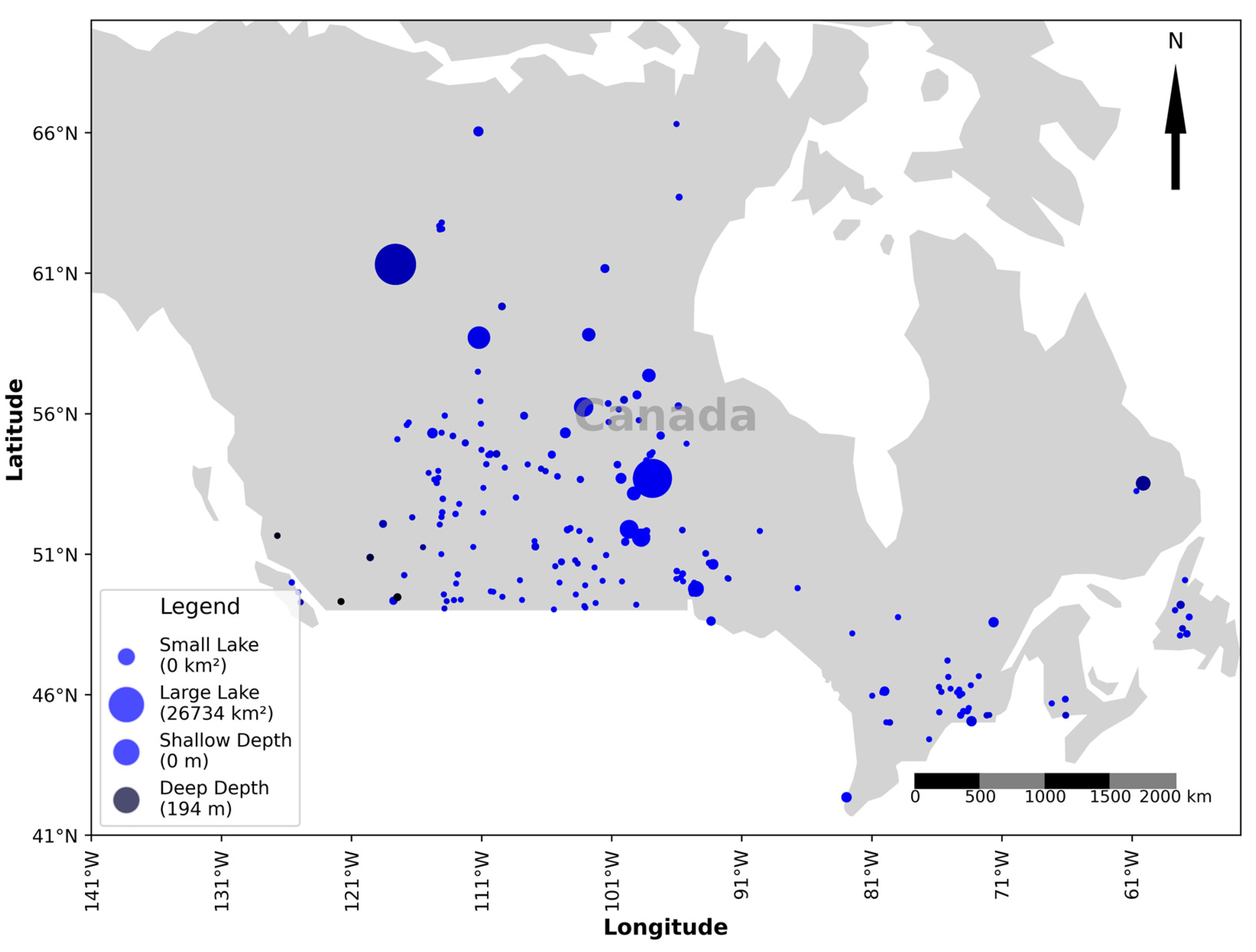
Figure 2.
Relationship between lake elevation and average depth for the 182 lakes analyzed in the study.
Figure 2.
Relationship between lake elevation and average depth for the 182 lakes analyzed in the study.
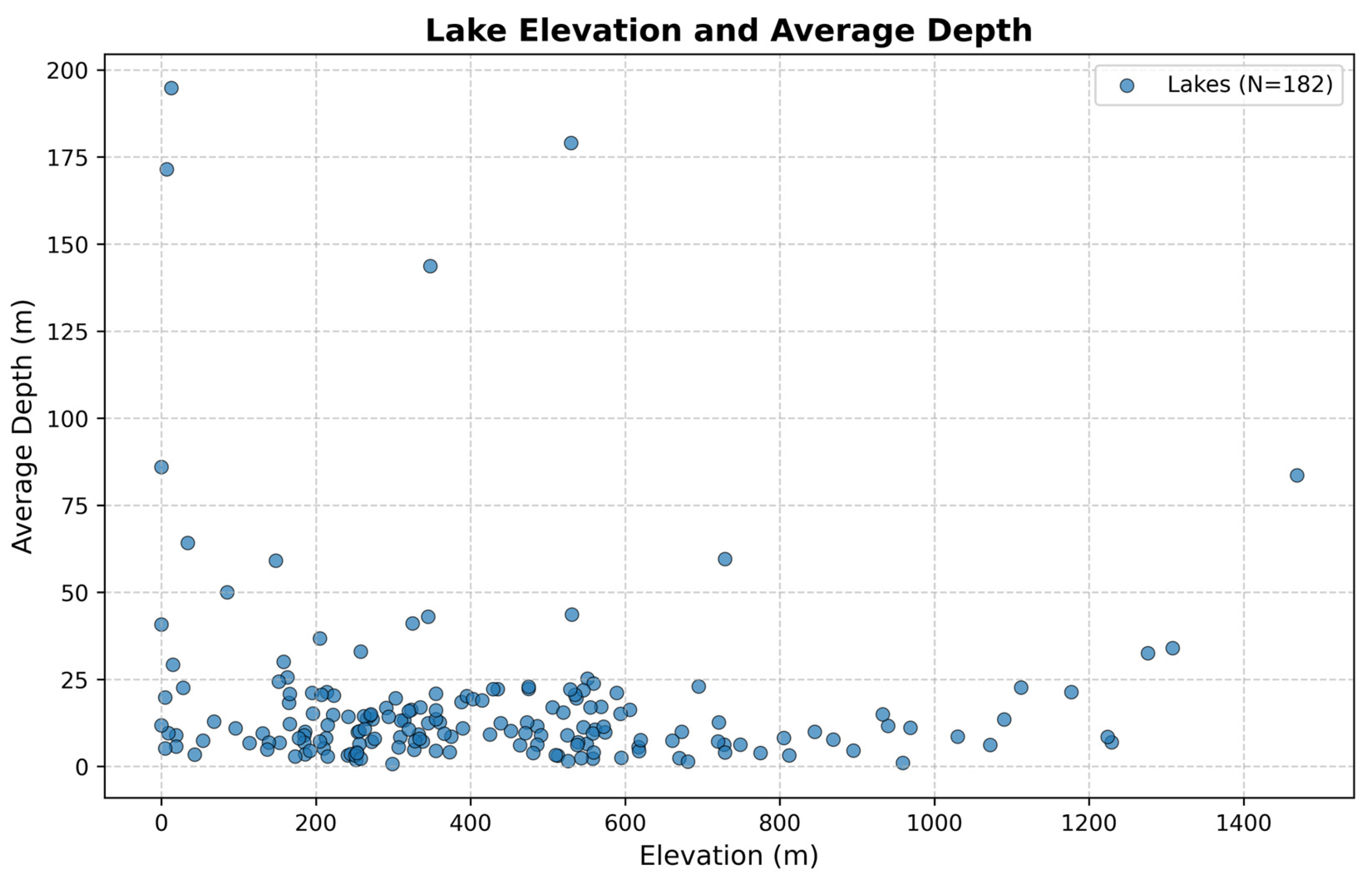
Figure 3.
Distance matrix of the 20 largest lakes.
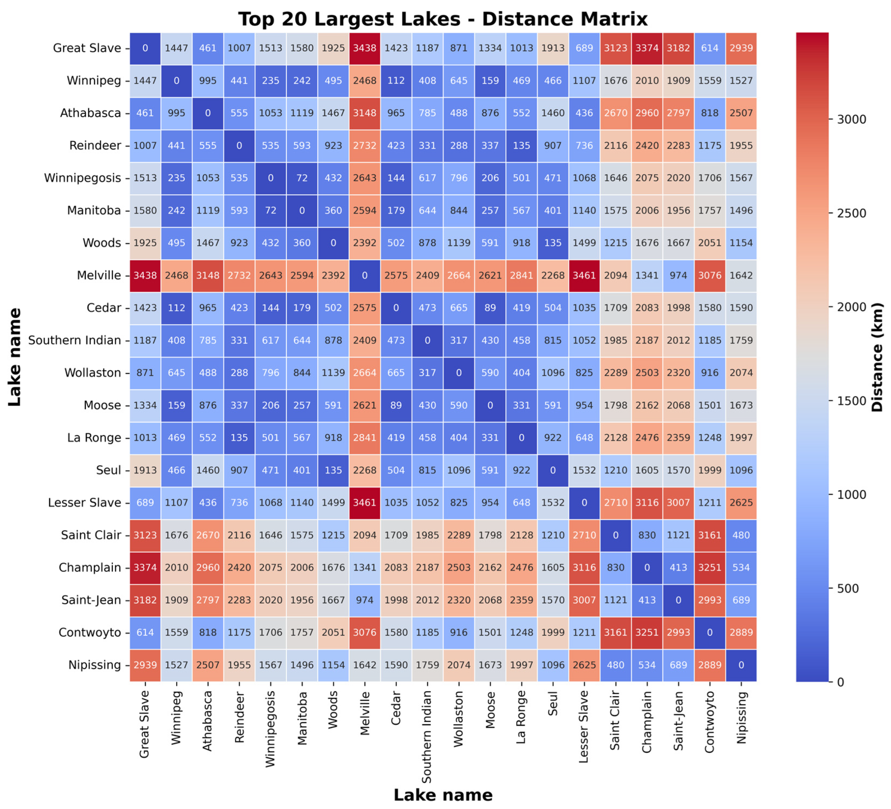
Figure 4.
Distribution of RMSE, MAE, and MBE values for both filtered and unfiltered ICESat-2-derived water levels compared to in situ gauge measurements.
Figure 4.
Distribution of RMSE, MAE, and MBE values for both filtered and unfiltered ICESat-2-derived water levels compared to in situ gauge measurements.
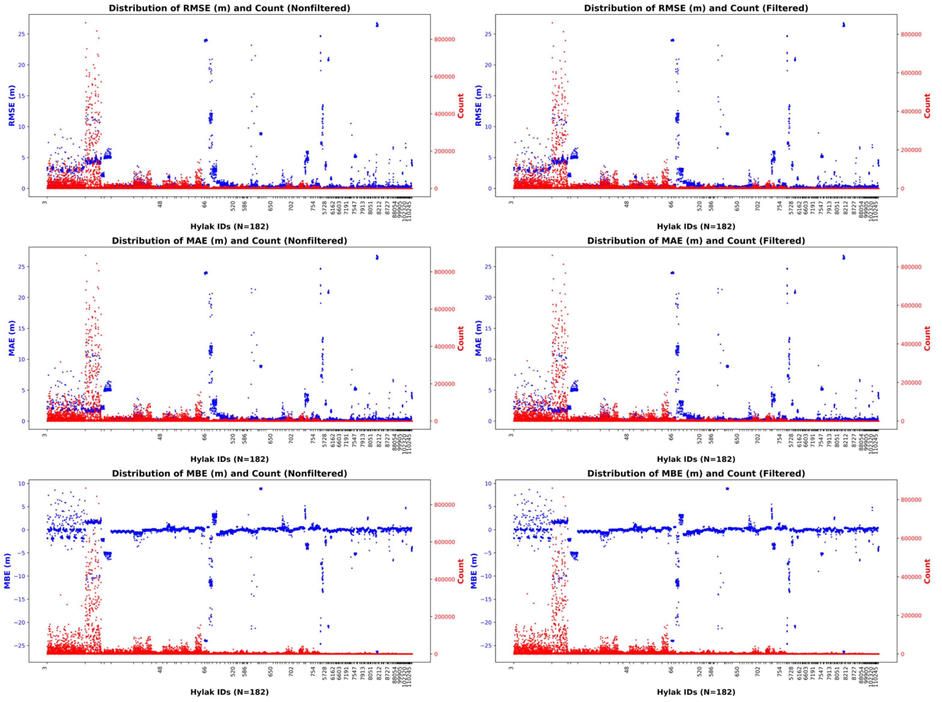
Figure 5.
Polar plots of RMSE, MAE, and MBE for the 20 largest lakes, comparing non-filtered (left) and filtered (right) datasets.
Figure 5.
Polar plots of RMSE, MAE, and MBE for the 20 largest lakes, comparing non-filtered (left) and filtered (right) datasets.
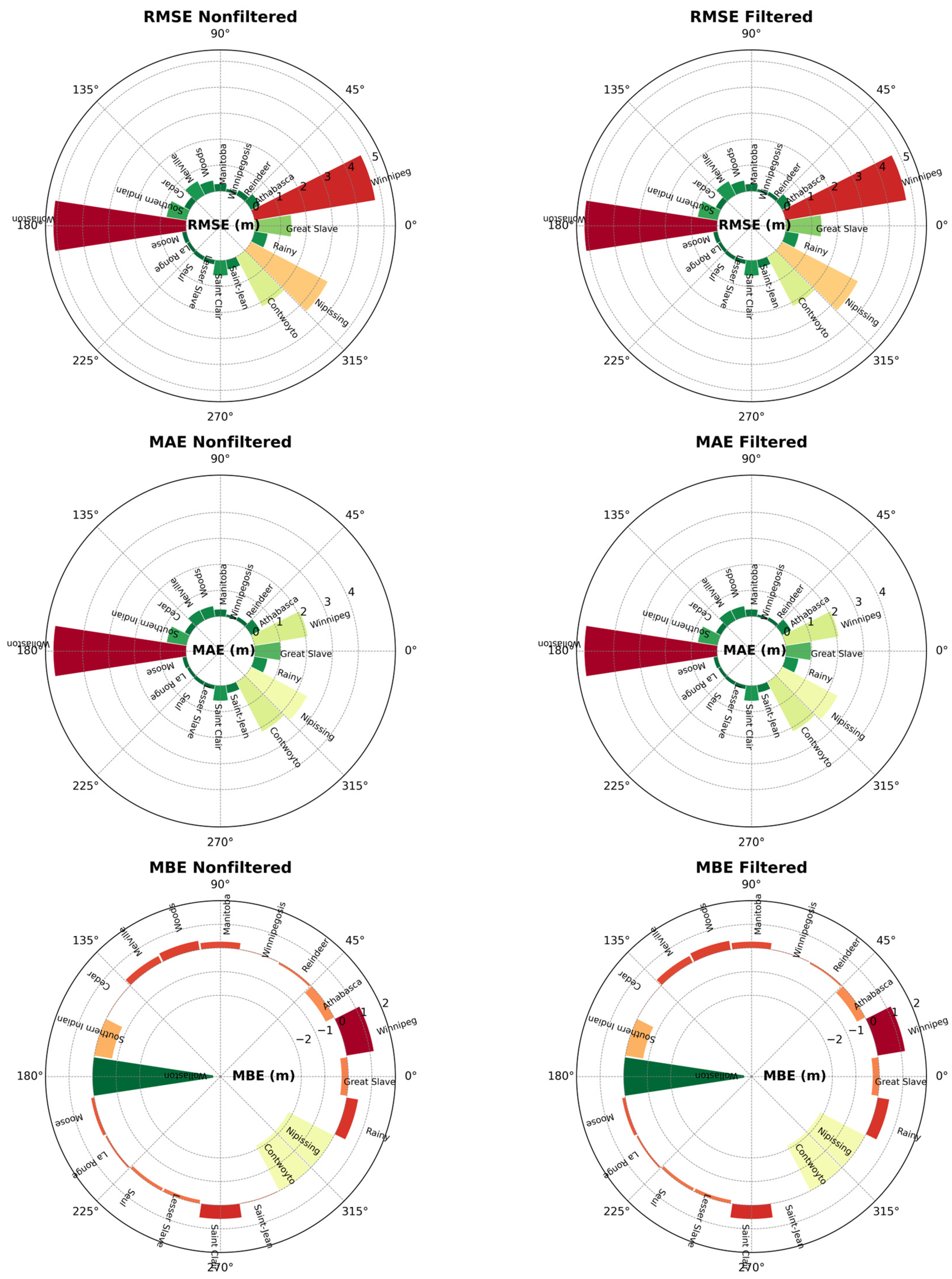
Figure 6.
Linear regression comparisons between ICESat-2-derived water levels and gauge measurements for unfiltered (left) and filtered (right) datasets.
Figure 6.
Linear regression comparisons between ICESat-2-derived water levels and gauge measurements for unfiltered (left) and filtered (right) datasets.
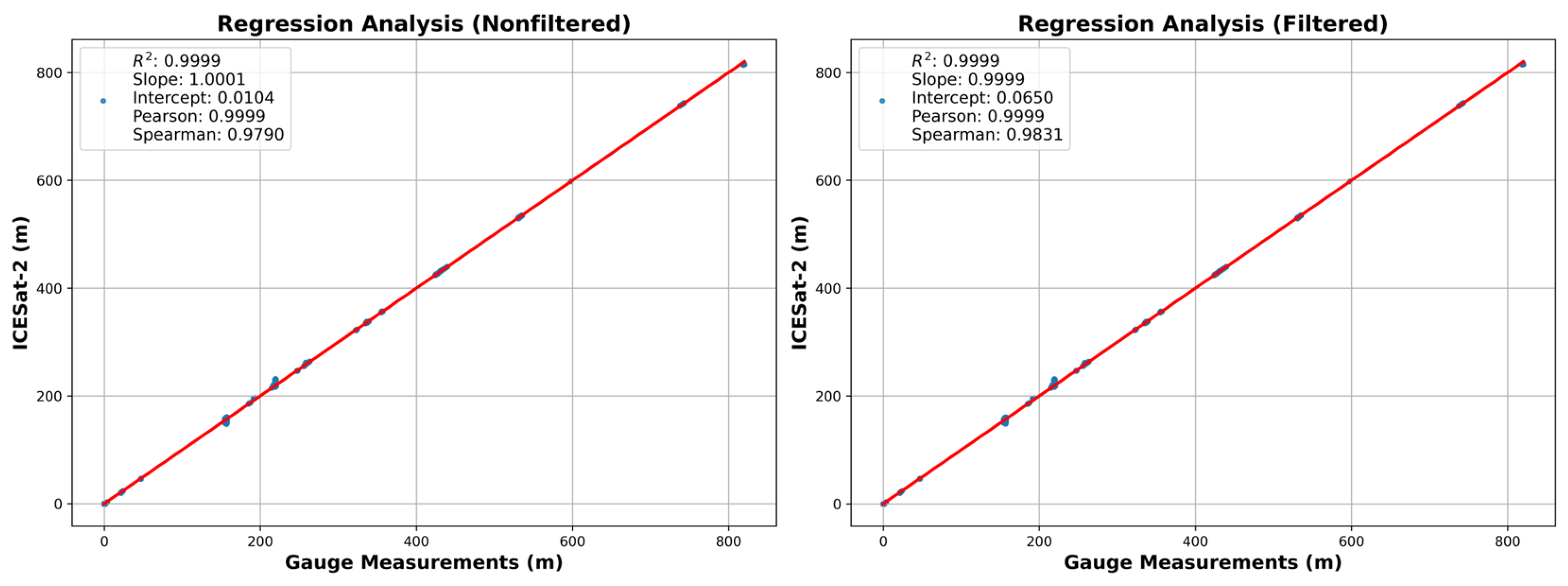
Figure 7.
Residual Distribution Analysis – Histogram, KDE, and Q-Q Plots for Unfiltered and Filtered Data.
Figure 7.
Residual Distribution Analysis – Histogram, KDE, and Q-Q Plots for Unfiltered and Filtered Data.
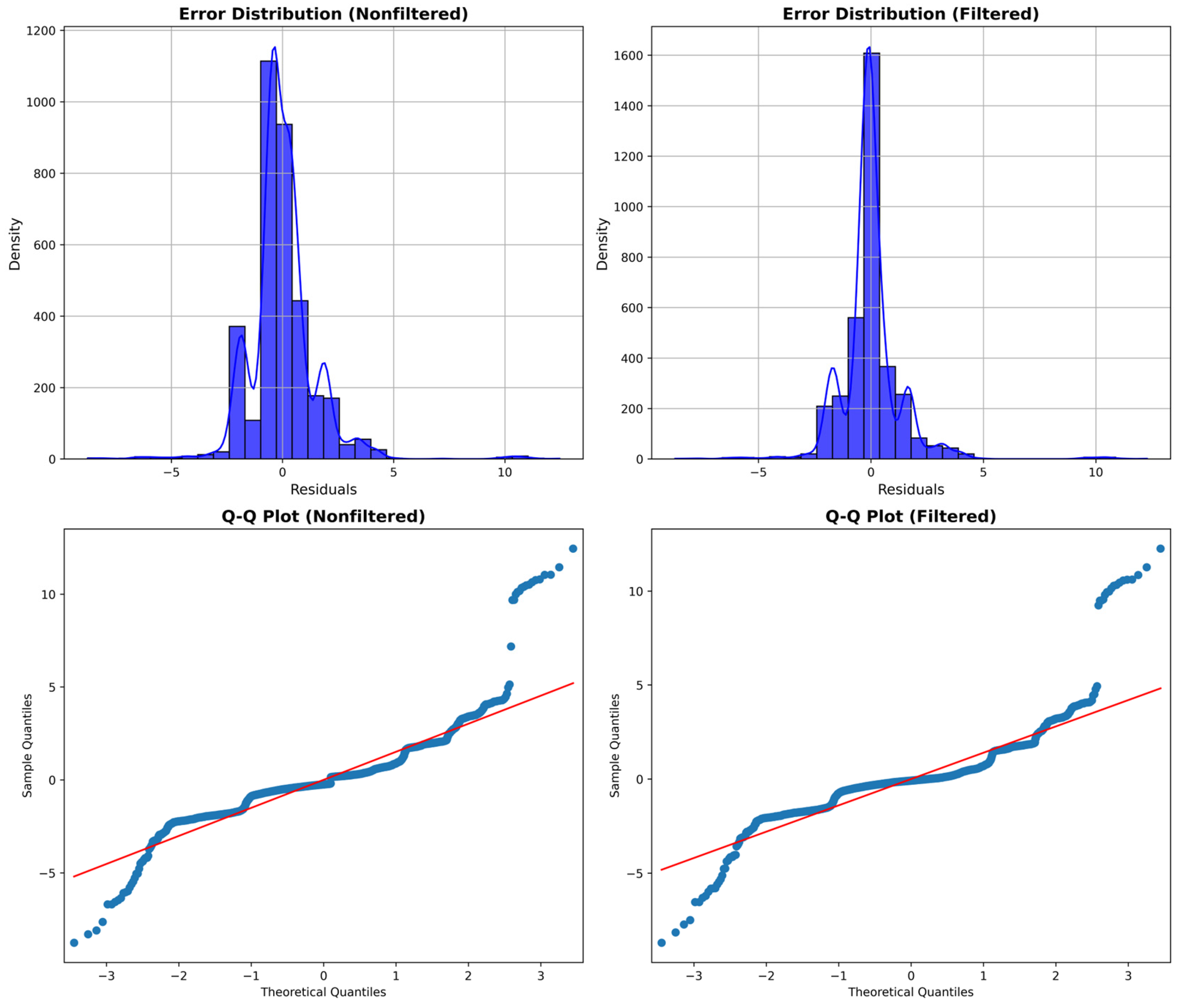
Figure 8.
Influence of Lake Characteristics on RMSE.
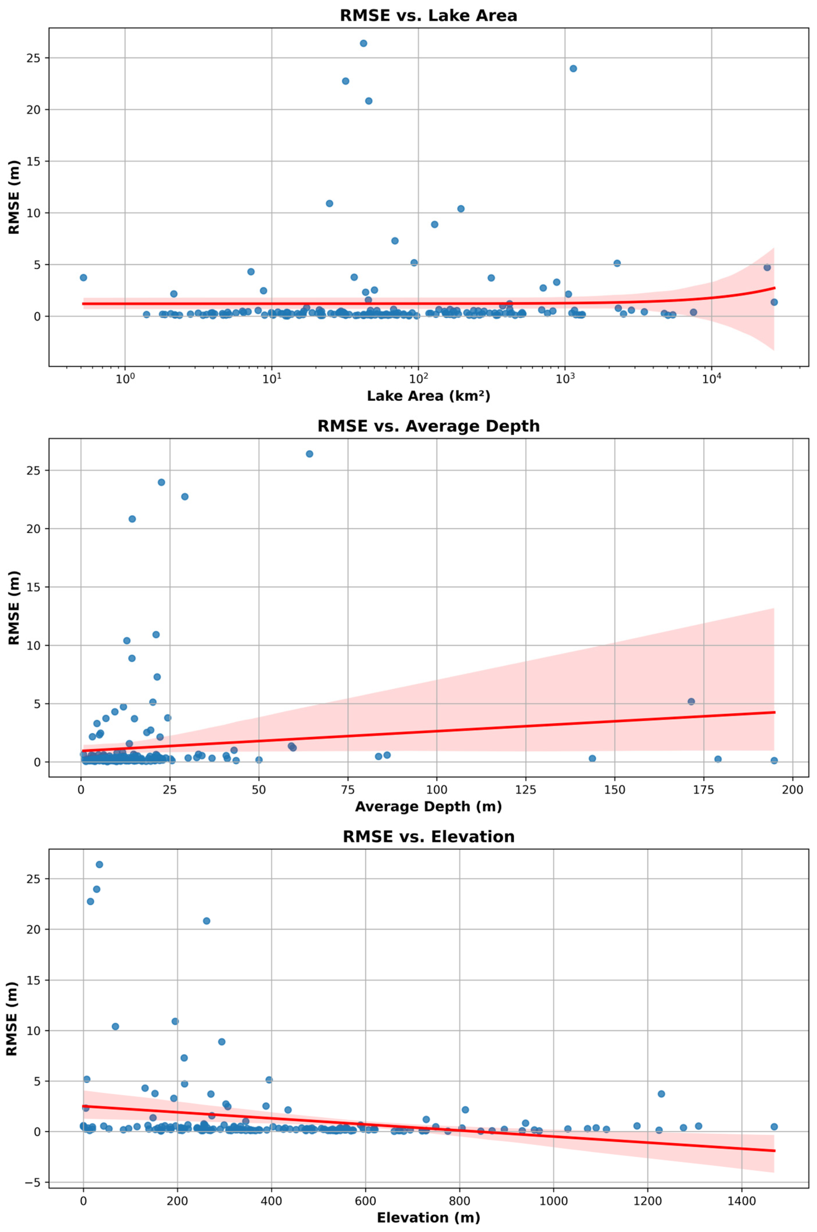
Figure 9.
Influence of Photon Density on RMSE.
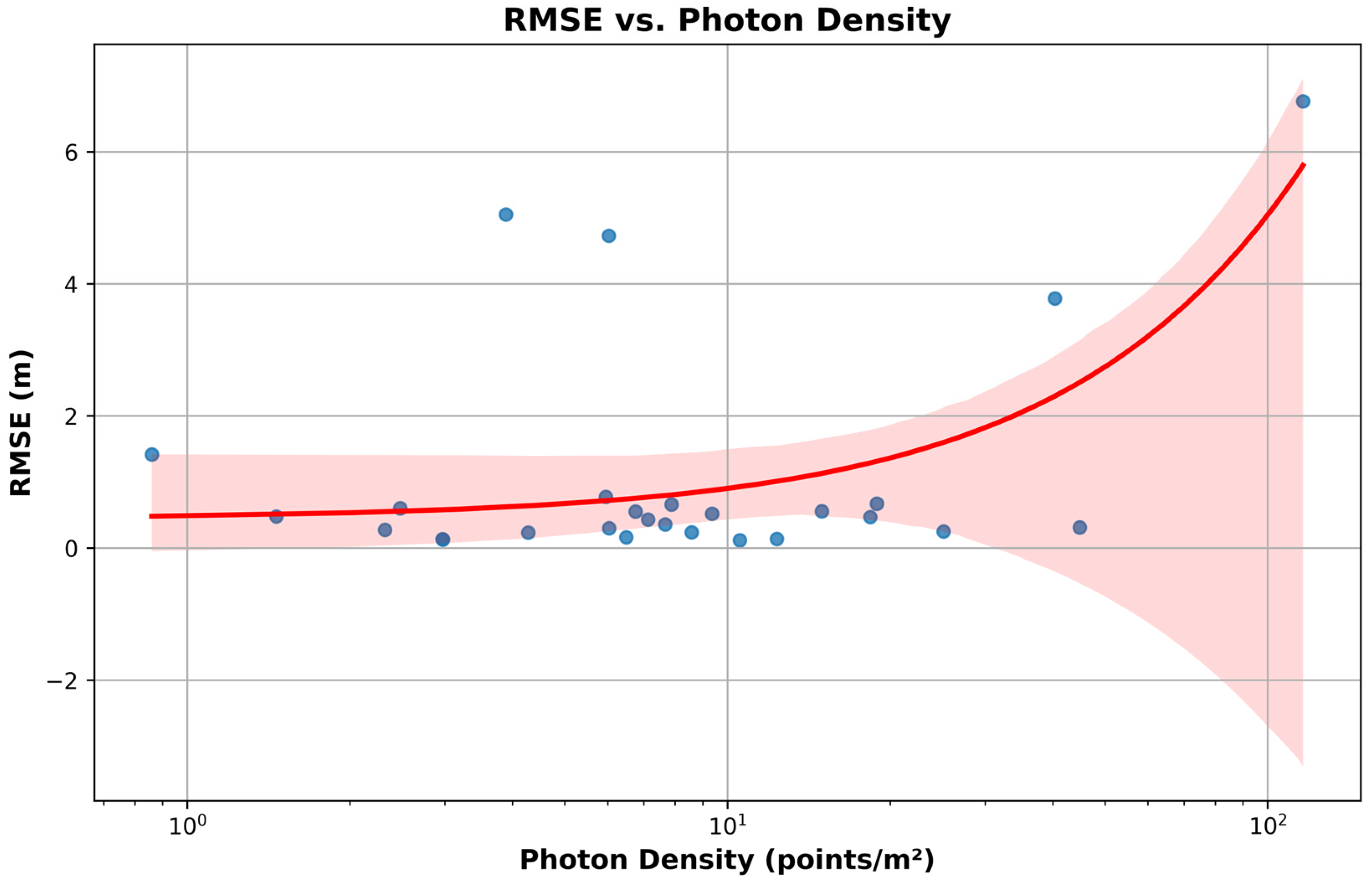
Figure 10.
Temporal Trends in Mean Orthometric Height of Lakes (2018–2024).
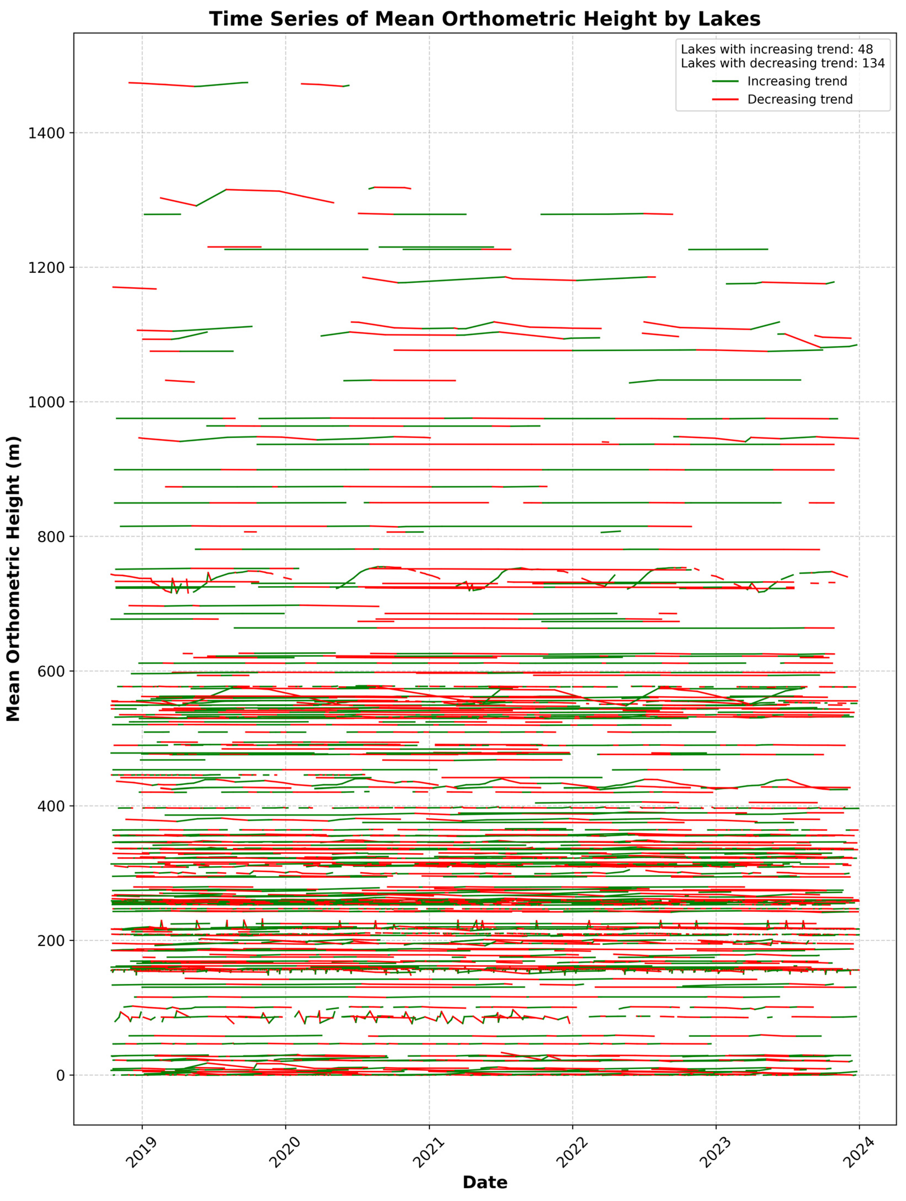

Table 1.
Summary of statistical analyses applied in this study.
| Analysis Type | Description | Metrics/Tests Used | Reference |
|---|---|---|---|
| Error Metrics | Quantifies discrepancies between satellite and gauge levels | RMSE (Eq. 3), MAE (Eq. 4), MBE (Eq. 5) |
[31,32] |
| Regression Analysis | Models the relationship between ICESat-2 and gauge data | β1(Slope), β0 (Intercept), R2 (Eq. 6) |
[33] |
| Correlation Analysis | Measures the strength of association between datasets | Pearson’s r (Eq. 7), Spearman’s ρ |
[34] |
| Error Distribution Analysis | Examines the nature and normality of error distributions | Histogram, KDE, Shapiro-Wilk Test |
|
| Temporal & Spatial Stratification | Evaluates error variation across different conditions | Daily boxplots, lake-specific groupings |
|
| Lidar Point Density Analysis | Assesses the relationship between point density and error metrics | RMSE, MAE comparison based on photon density |
Disclaimer/Publisher’s Note: The statements, opinions and data contained in all publications are solely those of the individual author(s) and contributor(s) and not of MDPI and/or the editor(s). MDPI and/or the editor(s) disclaim responsibility for any injury to people or property resulting from any ideas, methods, instructions or products referred to in the content. |
© 2025 by the authors. Licensee MDPI, Basel, Switzerland. This article is an open access article distributed under the terms and conditions of the Creative Commons Attribution (CC BY) license (http://creativecommons.org/licenses/by/4.0/).
Copyright: This open access article is published under a Creative Commons CC BY 4.0 license, which permit the free download, distribution, and reuse, provided that the author and preprint are cited in any reuse.


