
Submitted:
03 March 2025
Posted:
04 March 2025
You are already at the latest version
Abstract
In recent years, synthetic aperture radar (SAR) technology has been increasingly explored for automotive applications. However, automotive SAR images generated via the matched filter (MF) often exhibit challenges such as noisy backgrounds, sidelobe artifacts, and limited resolution. Sparse regularization methods ave the potential to enhance image quality. Nevertheless, conventional unweighted ℓ1 regularization methods struggle to address cases with radar cross section (RCS) distributed over a wide dynamic range, often resulting in insufficient sidelobe suppression, amplitude distortion, and inconsistent super-resolution performance. In this paper, we propose a novel reweighted regularization method, termed Multi-Segment-Reweighted Regularization (MSR), for automotive SAR image restoration. By introducing a novel weighting scheme, MSR localizes the global scattering point enhancement problem to the mainlobe scale, effectively mitigating sidelobe interference. This localization ensures consistent enhancement capability independent of RCS variations. Furthermore, MSR employs multi-segment regularization to constrain amplitude within the mainlobes, preserving the characteristics of the original response. Correspondingly, a new thresholding function, named Thinner Response Undistorted THresholding (TRUTH), is introduced. An iterative algorithm for enhancing automotive SAR images using MSR is also presented. Real data experiments validate the feasibility and effectiveness of the proposed method.
Keywords:
automotive SAR
; image restoration
; weighting scheme
; thresholding function
; consistent enhancement
; Multi-Segment-Reweighted regularization
1. Introduction
Compared to other widely used sensors such as Lidar and camera, automotive radar typically referring to millimeter wave (MMW) radar mounted on vehicles offers significant advantages in terms of low cost price and robustness even in adverse weather conditions or in dim nights. However, the limited azimuth resolution of automotive radar remains a notable drawback that impacts its overall performance [1]. To address the challenge of improving angular/azimuth resolution (AR) in side-looking automotive radar, synthetic aperture radar (SAR) technology has been increasingly explored and tested for automotive applications in recent years [2,3]. By mounting SAR on a moving vehicle platform, an equivalent long aperture of the radar array is achieved through coherent processing of signals collected during the vehicle’s motion. Automotive SAR images provide high resolution and visual clarity, making them particularly suitable for side-looking radar applications such as parking information perception [4], lane boundary detection [5], and automatic parking [6]. Unlike traditional SAR systems, which often focus on specific types of targets, automotive SAR is designed to handle more complex scenarios and diverse targets, including those with radar cross section (RCS) distributed over a wide dynamic range [7].
Matched filter (MF) algorithms, such as the range migration algorithm (RMA), are commonly employed to synthesize SAR images in automotive applications [8]. Automotive SAR images generated via MF often exhibit some limitations, including noisy backgrounds, sidelobe artifacts, and limited resolution. Sparse regularization methods have shown promise in enhancing image quality by adding sparsity of signals as prior knowledge [9,10,11]. A significant challenge in applying sparse signal processing techniques to automotive SAR imaging lies in the coupling of azimuth and range phase histories within the SAR geometry. Without decoupling these components, direct application of sparse methods is impractical [10]. Although an azimuth-range decoupling method has been proposed for automotive SAR sparse imaging from echo data [12], its computational complexity remains a limiting factor for its practical implementation.
To efficiently obtain sparse-enhanced SAR images, a sparse SAR imaging method based on complex images, modeled as unweighted regularization, was introduced in [13]. This method has been proven to effectively improve the quality of SAR images. However, when applied to scenarios with RCS distributed over a wide dynamic range, the conventional unweighted regularization approach exhibits several limitations, including insufficient sidelobe suppression, amplitude distortion, and inconsistent super-resolution performance. These issues have been highlighted in existing literature, such as [14]. Automotive SAR scenarios, characterized by diverse targets with varying RCS, are a prime example of such wide dynamic range cases [7]. When employing the unweighted regularization model for automotive SAR restoration, a critical limitation arises: the flexibility of regularization is only confined to the selection of regularization parameters. However, selecting a single parameter suitable for the entire SAR image with a wide RCS dynamic range is difficult. Parameters chosen to preserve the energy of weak scatterers’ mainlobes are often too small to effectively suppress sidelobes for strong scatterers, while parameters optimized for strong scatterers tend to overlook weak scatterers. Even when a trade-off parameter, such as the so-called "optimal parameter" discussed in [15,16,17], is selected, weak scatterers may be missed, and strong scatterers may still exhibit residual sidelobe artifacts. In summary, the simple unweighted regularization model is not applicable for automotive SAR applications.
A regularization penalty term with greater flexibility is essential to address the limitations of conventional methods. Existing penalty terms can be broadly categorized into two frameworks: reweighting frameworks and penalty modifying frameworks. Reweighting frameworks, as exemplified in [18,19,20,21], assign distinct weights to individual elements of the signal. The primary advantage of this approach lies in its ability to flexibly apply varying degrees of constraints to different signal components, enabling tailored regularization based on the specific characteristics of each element. On the other hand, penalty modifying frameworks, as exemplified in [22,23,24], replace the constraint with alternative forms of regularization. The primary advantage of this framework is its potential to recover signals more accurately, particularly when the modified penalty term perfectly reflects the statistical properties of the signal. Both frameworks provide distinct advantages, and their applicability is determined by the specific requirements and characteristics of the signal under consideration. Both frameworks offer unique advantages, and the choice between them depends on the specific requirements of processing and characteristics of the signal being analyzed.
In this paper, we propose a novel reweighted regularization method, termed Multi-Segment-Reweighted (MSR) regularization, for automotive SAR image restoration. MSR constructs its penalty term by integrating penalty terms from both reweighting and penalty modifying frameworks [18,19,22,23,24]. First, through an innovative weighting scheme, MSR localizes the global scattering point enhancement problem to the mainlobe scale, effectively mitigating the influence of sidelobes. The weighting scheme is inspired by methodologies in [18,20,21] and assigns weights proportional to adaptive filtering outputs that suppress sidelobes [25]. This localization ensures that MSR achieves consistent enhancement capability, independent on RCS variations. Then, MSR employs multi-segment regularization to constrain the amplitude within the mainlobes, preserving the characteristics of the original response. This approach leads to the introduction of a novel thresholding function, termed Thinner Response Undistorted THresholding (TRUTH), which is different from conventional thresholding functions in sparse signal processing [23,24,26,27,28]. The multi-segment strategy underlying this approach can be traced back to foundational works in [29,30]. By integrating these strategies, MSR provides an innovative solution for automotive SAR image enhancement, effectively addressing critical challenges such as sidelobe suppression, undistorted amplitude preservation, and consistent super-resolution performance.
The main contributions of this paper are summarized as follows:
- (1)
- A sparse SAR image enhancement method based on complex images is introduced for automotive applications. The limitations of the conventional unweighted regularization method are revealed, particularly in scenarios with radar RCS distributed over a wide dynamic range. The inconsistent resolution enhancement and amplitude bias of the conventional unweighted regularization method are quantitatively analyzed.
- (2)
- Existing frameworks for constructing more flexible penalty terms, reweighting and penalty modifying frameworks, are reviewed. A novel approach combining these two frameworks is proposed to leverage the advantages of both.
- (3)
- A novel image enhancement method, termed MSR regularization, is proposed for automotive SAR. MSR constructs its penalty term by integrating penalty terms from both reweighting and penalty modifying frameworks. On one hand, a novel weighting scheme is introduced, which localizes the global scattering point enhancement problem to the mainlobe scale, effectively suppressing sidelobes. On the other hand, a multi-segment regularization strategy is employed to eliminate distortion of the enhanced results. Correspondingly, a new thresholding function, the TRUTH function, is introduced as a fast solver for multi-segment regularization problem.
- (4)
- An iterative algorithm for enhancing automotive SAR images using MSR is presented. Real data experiments are conducted to validate the feasibility and effectiveness of the proposed method.
The remainder of this paper is organized as follows. Section 2 formulates the problem of automotive SAR image enhancement via regularization and introduces related works as a reference. Section 3 presents the proposed MSR method and its iterative algorithm. Section 4 showcases the results of real data experiments. Finally, Section 5 concludes the paper.
2. Problem Formulation and Related Works
2.1. Problem Formulation and Regularization Method
The degradation model of the low-quality SAR image can be expressed as:
where is the known low-quality SAR image generated via MF, is the high-quality image to be restored with enhanced features, and represents the difference between and . Here, , , and all share the same pixel dimensions of , where and denote the number of pixels in the azimuth and range directions, respectively.
The regularization-based method reconstructs high-quality signals by minimizing the sum of the signal adaptation error and the prior error. This can be formulated as:
where, denotes the Frobenius norm of the matrix, denotes the regularization parameter, and denotes the regularization term or penalty term, which is constructed based on prior knowledge of the signal characteristics. The first term ensures fidelity to the observed data , while the second term incorporates prior information to regularize the solution and enhance desired features.
The sparsity of signals is a widely utilized prior knowledge in numerous signal processing applications. Assuming that is spatially sparse, can be reconstructed by solving the following regularization optimization problem:
where, denotes the -norm of ,which counts the number of non-zero elements in ().
However, the regularization optimization problem is a nondeterministic polynomial-time hard (NP-hard) problem, which is almost impossible to be resolved. A relaxation strategy can be adopted, and the equivalent solution to the regularization can be approximately estimated by solving following regularization optimization problem:
where, denotes the -norm of , its value equals to the sum of absolute values of all elements in ().
The regularization optimization problem is also known as basis pursuit denoising (BPDN) problem, which can be resolved by existing optimization algorithms, such as Soft thresholding. The Soft thresholding estimation for image pixel can be expressed as:
where, denotes the positive part of a real number, equals x for or 0 for , denotes the sign function.
2.2. Limitations of Regularization Method for SAR Image Enhancement
In the case with wide dynamic RCS, the amplitudes of are assumed to span a large interval, such that .
It’s difficult to select an appropriate parameter for whole SAR image. If a large parameter is selected. let and denote the support set and its complement respectively. Some weak scatterers locate at are removed in the reconstruction. If a small parameter is selected to keep all scatterers maintained. Though, small parameter weaken constraints of sparse regularization term. As for most elements of , their amplitude are far greater than , . Their reconstruction can be approximatively expressed as:
The approximation means that most elements of the SAR image are almost not restored, which is unacceptable as well.
In addition, resolution of scatterers are enhanced inconsistently versus their amplitude. The point spread function (PSF) of ideal SAR images generated via the MF can be approximate as a bi-dimensional sinc function. The response of a scatterer with amplitude after the regularization estimator tends to be sharpened. By fitting the sinc function with a quadratic function , the 3dB mainlobe width of the estimated response can be simply calculated as:
where, represents the theoretical resolution of the system. The formula illustrates that weaker scatterers, characterized by smaller amplitudes, exhibit finer local responses when estimated via regularization. As a result, the apparent resolution of weaker targets appears higher. However, this inconsistent sharpening also implies non-recoverable distortion and energy loss in the local response, which can compromise the accuracy and reliability of the reconstructed image.
The expectation of estimated amplitude can be separately expressed as:
This indicates that the amplitudes of the scatterers are systematically underestimated. Unfortunately, the amplitude bias is nonlinear with respect to the true amplitude, which reduces the quantization accuracy of the SAR image. The statistical characteristics of the target’s RCS may be altered, leading to potential distortion of responses.
In summary, when applied to scenarios with RCS distributed over a wide dynamic range, the unweighted regularization method results in SAR images with several limitations: insufficient sidelobe suppression, amplitude distortion, and inconsistent super-resolution performance.
2.3. Related Works About Reweighted Regularization
General linear observations can be described in matrix form as:
where, denotes the vector of observation data, denotes the signal vector to be estimated, denotes the measurement matrix or observation matrix.
Conventional unweighted regularization method recovery sparse signal by solving the optimal solution of the penalized least square optimization problem as:
Using the penalty function to approximate the penalty function is not always the optimal choice. For example, a log-sum penalty function has been demonstrated to offer superior approximation capabilities. The penalty function, penalty function, and log-sum penalty function for a single variable t can be respectively represented as:
where, denotes a a small positive constant.
An abridged general view illustrating the difference between the and the penalty terms is shown in Figure 1. The figure also demonstrates that the penalty function is more accurately approximated by the log-sum penalty terms than by the one [18]. This highlights the superior ability of the log-sum penalty function for sparse signal recovery.
When the log-sum penalty function is used in the recovery of sparse signals, the corresponding optimization problem can be formulated as:
A strategy with weights inversely proportional to the true signal magnitude is proposed in [18]. After applying the weighting, the problem in Equation (12) can be equivalently solved by addressing the following regularization optimization problem:
where, is a small positive constant, denotes the weight of .
A similar log-sum family penalty function is adopted for SAR sidelobe suppression in[31]. In order to facilitate the comparison, only its one-dimensional simplified form is represented here as:
This log-sum penalty function excels in sidelobe suppression and mainlobe preservation. Similar to the equivalence between Equation (12) and Equation (13), the problem in Equation (14) can also be equivalently transformed into a reweighted regularization (RL1) optimization problem:
Another framework for weighting schemes is introduced in the adaptive lasso technique [32]. The adaptive lasso addresses the following reweighted regularization problem:
where, is a positive constant.
The above-mentioned weighting schemes, their equivalent penalty problems, and their related adaptive lasso forms are summarized in Table 1. This table also includes several other commonly used existing weighting schemes for reference.
The aforementioned weighting schemes are based on basic operations involving signal amplitude. In contrast, another category of methods incorporates image convolution operations. For instance, Zhang et al. [20] propose a novel convolutional reweighted scheme, where weights are assigned inversely proportional to the outputs of a smooth filtering process.
where, is a small positive constant, denotes a filter kernel smoothing the signal, denotes the convolution operation between and .
The convolutional reweighted scheme is capable of simultaneously achieving sparse signal recovery and region enhancement. For ease of comparison with other weighting schemes in subsequent discussions, we designate this convolutional reweighted scheme as "Weighting Scheme 7 (WS7)".
2.4. Related Works About Modified Penalty Term
By minimizing norm of , one can obtain the least squares error . The least squares estimation can be regarded equivalently as . The penalized least square cost function can be expressed as:
where, denotes the transformed observation vector, denotes the reconstructed signal of least square method, denotes the penalty functions, which are allowed to depend on parameters .
The analytical form first introduced in [19] provides a component-wise form for regularization. When the penalty functions for all coefficients are variable and depend on parameters , the term can be denoted by . Then, the component-wise form regularization can be expressed as:
When the penalty term is determined, thresholding methods can be employed to reconstruct the signal. For example, can be expressed in the form of a discontinuous penalty function, such as:
where, is a regularization parameter set containing only one element. The solution to the discontinuous penalty function in Equation (20) takes the form of the Hard thresholding function [26,33]. The Hard thresholding function can be expressed as:
For another example, in norm regularization is presented as the product of regularization parameter and absolute value of signal:
The Hard and Soft thresholding functions are widely used in sparse signal processing. A visualization of these two functions is shown in Figure 2. Each thresholding function has its own advantages and disadvantages: The Hard thresholding function preserves the amplitude of signal components above the threshold without bias. But it can introduce higher estimation error and is often highly sensitive to noise and threshold selection, leading to potential instability in sparse signal recovery; The Soft thresholding function provides a more stable and continuous estimation of the signal, and it generally performs better for overall signal estimation. But it introduces amplitude bias, which can distort the true amplitudes of the recovered signal.
If a constant exponential operation is applied to the amplitude in Equation (22), the penalty function becomes more generalized, corresponding to regularization. This can be expressed as:
where, make the penalty term still retain sparse constraint capability. Among all cases, the is especially noteworthy for its excellent and non-excessive sparse constraint performance [22].
Xu et al. [28] propose a fast thresholding solver, the Half thresholding function, for norm optimization problem. The Half thresholding function can be expressed as:
The Half provides a smoother transition than the Hard while introducing less bias than the Soft, as illustrated in Figure 3(a).
Similar as the Half thresholding function, nonnegative Garrote another compromise solution [35]. The nonnegative Garrote, recorded as Garrote+, can be expressed as:
The Garrote+ thresholding function lacks a model foundation, so we will not discuss it here for more details. One may naturally consider the composite scheme of in Equation (19) and Equation (22) by segmenting and piecing segments together:
It’s solution takes the form of mixture of the Hard and the Soft [24], abbreviated as Mix thresholding function shown in Figure 3(b). It can be expressed as:
The minimax-concave (MC) penalty is a transitional method upgraded on the basis of the simple composite scheme. MC penalty term use double regularization parameters, where , .
It’s solution takes the form of mixture of the Hard thresholding function and the Soft one as well but with a transitional slope as shown in Figure 3(c) [23]. The transition version mixture is named as the semi-Soft or the Firm, which can be expressed as:
Smoothly clipped absolute deviation (SCAD) penalty can be regarded as another transitional method. SCAD penalty term use double regularization parameters as well and build transitional penalty term even more more delicately as:
where, .
Unlike MC penalty, SCAD penalty has continuous derivatives [19], expressed as:
It’s solution also takes the form of mixture of the Hard thresholding function and the Soft one but with a more delicate transitional slope as shown in Figure 3(d). The thresholding function for SCAD penalty can be expressed as:
2.5. Summary of Related Works
Existing penalty terms can be divided into two categories: reweighting framework and penalty modifying framework. There are connections and differences between these two.
Connections between these two frameworks reveal that some reweighting frameworks and penalty modifying frameworks are equivalent, as listed in Table 1. The modified forms of penalty functions can inspire the development of new weighting schemes. For instance, even the most primitive weighting scheme was inspired by the log-sum penalty [18].
Differences between these two frameworks lie in their approaches to modifying the model, their respective advantages, and their solving methods: Reweighting framework directly assign different weights to each element of the signal. It flexibly applies varying degrees of constraints to different components of the signal, enabling adaptive regularization. And its solution process is similar to solving an unweighted regularization problem, except that weights are updated iteratively and multiplied by the signal components; Penalty modifying framework replace the constraint with alternative forms of penalty terms. It tends to recover signals more accurately when the modified penalty term aligns well with the statistical characteristics of the signal. And its solution is typically expressed as a thresholding function that depends on the specific form of the penalty term.
These differences highlight the complementary advantages of the two frameworks. Reweighting frameworks excel in adaptability and flexibility, while penalty modifying frameworks offer improved accuracy when the penalty term is well-matched to the signal’s properties. Combining insights from both frameworks can lead to more robust and effective regularization techniques for sparse signal recovery.
3. Multi-Segment-Reweighted Regularization and Iteration Algorithm
3.1. A Combination Framework
In the previous section, the reweighting framework and penalty modifying framework were reviewed as approaches to constructing more flexible penalty terms. In this paper, we aim to develop a combined framework that integrates the advantages of both frameworks.
According to the reweighted regularization model, can be reconstructed in reweighting framework by solving the following optimization problem:
where, denotes the weights matrix, ⊙ denotes the Hadamard product of matrices.
According to the modified penalty term model, can be reconstructed in penalty modifying framework by solving the following optimization problem:
where, denotes penalty term selected specially for SAR image enhancement applications.
Combining the above two equations, one can build a combination framework. Then, can be reconstructed in the combined framework by solving the following optimization problem:
A novel image enhancement method named as MSR for automotive SAR is proposed. On the one hand, a novel weighting scheme used in MSR is indicated. The novel weighting scheme localizes the global scattering point enhancement problem to the mainlobe scale, effectively suppressing sidelobes. On the other hand, multi-segment regularization strategy is adopted to remove distortion of enhanced results. Correspondingly, a novel thresholding function TRUTH is revealed. Details of the novel weighting scheme and the multi-segment regularization strategy are revealed in the next two subsections separately.
3.2. weighting Scheme for Consistent Enhancement
In [18], the weights were inversely proportional to the true signal magnitude, so that the parts of the signal with different amplitudes are normalized. This kind of weighting scheme is suitable for signal processing applications where the unit response is approximately an impulse function. As for accurate SAR applications, the unit response at the local scale can not be regarded as a impulse function anymore. The mainlobe of the unit response is widened and the sidelobes appear to leak the energy of the response. Therefore, we suggest an amplitude normalization weighting scheme that the weight for image pixel can be expressed as:
where, denotes the local peak amplitude of the lobe where the pixel is located. Let the entire weight matrix be denoted as .
Although the above weights can normalize mainlobes of responses, unfortunately, the sidelobes are also normalized simultaneously, which is revealed in Figure 4(b). Therefore, we suggest an extra weight to suppress sidelobes as:
where, denotes a bi-dimensional filter kernel suppressing sidelobes, weighted result of in Equation (39) is revealed in Figure 4(c).
Basic can take the values calculated in [25]. In cases of high sampling rate and fine image grid, exhibit pixel size of , where and are integer part of resolution to grid ratio, , . is with only a few nonzero coeffience which can be adaptively calculated pixel by pixel:
3.3. Multi-Segment Regularization
Inspired by the penalty function with continuous derivatives in [19], we propose a penalty function with approximately continuous derivatives:
where, is index of P regularization parameters , (), is a parameter adjusting the super-resolution factor of the result, whos value satisfies , and denote the response function of the mainlobe and its inverse function. In SAR application, usually presents or approximates the form of a sinc function.
The solution of Equation (42) also takes the form of multi-segment form. Examples can be found in Figure 5. Since the thresholding function is dedicated to enhancing lobes into thinner response without distortion, we name it as Thinner Response Undistorted THresholding (TRUTH). The TRUTH function can be expressed as:
If the interval between P points is fixed, such as are selected at equal intervals, then the threshold function can have a fixed form. The main parameters that affect the thresholding function are P and .
P determines the number of segments, and the larger the P, the more refined the model becomes, resulting in a thresholding function that better fits the smooth solution. For example in a fixed task, we fix , such as , and examine the variation of the thresholding function versus P. Figure 5 shows examples of . It can be observed that as P increases, the threshold function of the step sample becomes closer to a smooth thresholding function that is independent of the value of P. This smooth thresholding function can be expressed as:
is a task dependent parameter, and the larger its value, the higher the super-resolution factor required to be improved. Naturally, the larger value, and the further the thresholding function deviates from the diagonal. Figure 6 shows examples of .
3.4. Iteration Algorithm
We propose a iterative algorithm that alternates between estimating penalized signal and updating the weights, which is similar as the iterative algorithm in [18]. As for general problem in Equation (37), the main steps of the iterative algorithm are listed as follows:
- Set the iteration count k to zero and initialize ;
- Update the weights from according to the designed weighting scheme;
- Solve the reweighted regularization minimization problem:
- Terminate algorithm when update of converges or when k attains maximum number of iterations. Otherwise, k plus one and go to step 2.
As for specific problem in of our MSR regularization with weighting scheme in Equation (41) and penalty satisfies Equation (42), the main steps of the iterative algorithm are listed in Algorithm 1.
| Algorithm 1 Iteration Algorithm for Enhancement of Automotive SAR Image via MSR. |
|
Input: RMA recovered SAR image .
Initial: Model parameter , Update step size , Convergent tolerance , Iteration count , Maximum iterative steps , Thresholding function , Initial resorted image .
while and do
end while
Output: Restored SAR image .
|
The details of Algorithm 1 are explained as follows: The TRUTH thresholding function is built in advance, so that the corresponding thresholding operation can be implemented in practice through a lookup table; The local peak amplitude of the lobe can be obtained by continuous detecting maximum value among neighborhoods element by element.
4. Real Data Experiment
4.1. Experiment Setup
In this section, we validate the efficiency of our method in real data experiment with automotive SAR images. The real data in this paper is measured with SSAR (short-range SAR imaging radar), which is a 79 GHz SAR system design by Beijing Autoroad [36].
The echo data is measured in a parking lot scenario, as illustrated in Figure 7(a). The SAR image, shown in Figure 7(b), is coarsely focused using the RMA with a spatial coverage of . The resolution of the image is , providing a detailed representation of the scene for further analysis and enhancement.
The SSAR system is equipped with real-time signal processing module and SAR images display module. However, to verify and evaluate the novel proposed method, results of experiments in this paper are conducted on a workstation of 2.60-GHz Inter Core i7-9750 CPU with 8GB memory. The algorithms are implemented in MATLAB 2016.
4.2. The Outperformance of Our Weighting Scheme
Firstly, we enhance the automotive SAR image using the conventional unweighted regularization method, and the results reveal the limitations of the unweighted regularization method in processing SAR images with RCS distributing within a wide dynamic range. Then, we apply our proposed weighting scheme into the RL1 framework to obtain restored automotive SAR images, and compare its result with unweighted and several existing weighting schemes to demonstrate the outperformance of our proposed weighting scheme.
When enhancing the automotive SAR image using the conventional unweighted regularization method, one must first choose a suitable regularization parameter , which is the key parameter affecting the enhancement results. One of the most widely accepted parameter selection methods is selecting the corresponding to the corner point of the L-curve [15,37]. The L-curve in the conventional unweighted regularization denotes the versus . Each point on the L-curve corresponds to a specifically selected regularization parameter value.
Figure 8 shows the L-curve and metrics of norm regularization results with different selected with the SAR image of the Area1 in Figure 7(b). The L-curve is drawn with , and the optimal parameter value of is selected at the corner marked as red circle ∘, where . Form the trend of metrics versus , one can find that the so-called optimal regularization parameter value corresponding to the corner point is just a compromise choice. When is selected, the energy of the highest sidelobe still remain about , which means the ability of unweighted regularization to suppress sidelobes is very limited. And at this point, the elimination of residual background peaks is not sufficient, and the target scatters are not well preserved. This results in a reduction in both the absolute number and the proportion of effective point clouds corresponding to target scatterers. Such a reduction can degrade the quality and accuracy of the reconstructed SAR image, particularly in applications requiring precise target detection and characterization.
Figure 9 shows the local enlarged image of Area1 and its enhanced results via unweighted norm regularization with different selected, . From the result shown in Figure 9(b), the regularization with a small parameter reserves target scatters even the weak contour points well, but suffers from poor performance of sidelobe suppression. From the result shown in Figure 9(d), the regularization with a large parameter suppresses sidelobes well, but suffers from missing the weak contour points of the target. From the result shown in Figure 9(c), the regularization with a compromise parameter suffers from both of insufficient sidelobe suppression and weak contour points missing but both at a less serious level.
From these results above, it can be concluded that enhanced results via unweighted regularization is limited when encountering cases with RCS distributing over a wide dynamic range, which echoes the analysis in section 2.2.
Our proposed weighting scheme is applied to RL1 framework, and it’s expected to break the above limitations of unweighted regularization. To demonstrate the outperformance of our weighting scheme, we compare its result with constant weighting scheme (WS1) and several existing weighting schemes (WS2, WS3, WS6, WS7) mentioned in section 2.3. Weighting schemes (WS4, WS5) are not selected since they both assign too small weights to the mainlobe elements, which is not conducive to maintaining the mainlobes. As a typical sidelobe suppression algorithm, SVA is also adopted as a reference.
Figure 10 shows the enhanced results of Area1 SAR image. The enhanced result via SVA partially suppresses sidelobes and reserves target scatters, which is shown in Figure 10(a). And the enhanced results via RL1 with weighting scheme (WS2, WS3, WS6, WS7) shown in Figure 10(b∼e) are very similar with enhanced result via unweighted with weighting scheme (WS1) in Figure 9(c). The limitations of unweighted regularization, particularly its poor performance in simultaneously suppressing sidelobes and preserving weak contour points of the target, also negatively impact the results of reweighted (RL1) regularization with existing weighting schemes (WS2, WS3, WS6, WS7). The enhanced result via RL1 with our weighting scheme shown in Figure 10(f) not only effectively suppress the sidelobes near high amplitude scattering points, such as point P1, but also more completely preserve low amplitude scattering points, such as point P2∼4.
Metrics of RL1 automotive SAR image enhanced results with different weighting schemes are calculated and listed in Table 2. Image entropy (IE) and image contrast (IC) are adopted to evaluate the overall quality of enhanced images. Equivalent number of looks (ENL), radiometric resolution (RaRes) and target to background ratio (TBR) are adopted to evaluate the radiation characteristics of enhanced SAR images [38]. The number of residual background peaks and the number of reserved target scatters are adopted to evaluate the quality of peak point cloud images. The peak sidelobe ratio (PSLR) and integral sidelobe ratio (ISLR) at point F1 along range and azimuth directions are adopted to evaluate the sidelobe suppression performance.
As shown in Table 2, RL1 with our weighting scheme suppresses sidelobes completely, so that TBR, ISLR and PSLR in result of RL1 with our weighting scheme obtain infinite optimal values. Compared to the previous weighting schemes with performance metrics of IE, IC, ENL, RaRes, , , ISLR and PSLR, RL1 with our weighting scheme outperforms RL1 with other weighting schemes.
4.3. Undistorted Enhancement Ability of TRUTH Function
The previous subsection demonstrated the superior performance of our proposed weighting scheme, which is adopted in this subsection. Here, we validate the undistorted enhancement capability of the proposed multi-segment regularization. Specifically, we investigate how the performance of the multi-segment regularization varies with the number of segments P. Since different forms of penalty terms lead to different thresholding functions, we compare the proposed TRUTH function with existing thresholding functions to highlight the advantages of our multi-segment penalty term.
As shown in Figure 11, the local enlarged image of Area2 undergoes a sequential process of resolution degradation by discarding a portion of the 2D spectrum, followed by resolution re-enhancement through the MSR regularization. Directly evaluating the performance of results corresponding to different P values from the enhanced images is challenging. Instead, attention can be focused on the local representation of the image, where subtle distortion become more apparent.
As shown in Figure 12, the contour plots, range profiles, and azimuth profiles of the point P1, the point with strongest amplitude in the enhanced results, via MSR are visually analyzed. From the contour plots in Figure 12(a∼d), it is evident that the recovered mainlobe becomes progressively smoother as the P value increases. This indicates that segment effects are increasingly eliminated in the enhanced results, leading to a more continuous and natural representation of the target. From the range profiles in Figure 12(e∼h) and azimuth profiles in Figure 12(i∼l), it can be observed that the recovered amplitudes for small P values exhibit a distinct stair-step-like clustering phenomenon, which is a clear indication of distortion. As the P value increases, this clustering phenomenon gradually diminishes, and the enhanced amplitudes increasingly converge toward the true magnitudes.
The root mean square error (RMSE) and the structure similarity (SSIM) can be adopted as metrics to to evaluate the performance of the method [39]. In order to clarify the relationship between thereconstruction distortion and the segments number in the MSR model, We plot the RMSE and SSIM of MSR enhanced results versus segments number P, which is shown in Figure 13. Based on the results and trends in the figure, we suggest that the number of segmented number P should be at least 512, so that the restorations can achieve sufficiently small errors () and distortions that no longer decreases ().
The above results reveal that our MSR method is efficient and converges with respect to P. Then, we compare the TRUTH function with existing thresholding functions to showcase the advantages of our proposed multi-segment penalty term. As references, the thresholding functions the Hard, the Soft, the Half, the Garrote+, the Mix, the Firm and the SCAD mentioned in section 2.4 are all adopted as substitutes of TRUTH function in Algorithm 1. The parameters corresponding to each thresholding functions are adjusted so that their resulted mainlobes have the same energy value. Then, their results are compared with the result of our TRUTH function.
It is difficult to directly distinguish differences and evaluate performances of different thresholding functions from the enhanced images. One can focus on the local representation of the image again. As shown in Figure 14 and Figure 15, the range and azimuth profiles of the point P1 in the enhanced results are revealed visually. Among all these results, our TRUTH function is the only one that neither produces peak amplitude bias nor significant mainlobe distortion.
With amplitude bias, RMSE and SSIM adopted as metrics again, we calculated the metrics of MSR automotive SAR image enhancing with different different thresholding functions. The values of metrics are listed in Table 3. As for the bias values, the TRUTH thresholding function is verified as amplitude unbiased, as well as existing ones including Hard, Mix, Firm and SCAD. As for the RMSE values, the TRUTH thresholding function show outperformance than existing ones in restoring SAR images with lower error. As for the SSIM values, the TRUTH function enhancing the image of the point target with SSIMs, which are higher than the results of other thresholding functions. Therefore, the result of our TRUTH function shows the minimum distortion than the other ones.
4.4. Consistent Enhancement Ability of MSR Regularization
In the previous two subsections, we conducted comparisons and experiments using actual data to demonstrate the advantages of our weighting scheme and the undistorted enhancement capability of the multi-segment regularization. Next, we can integrate these components into a complete Multi-Segment-Reweighted regularization method and evaluate its performance in enhancing automotive SAR images.
The restorations of Area2 are shown in Figure 16. Both RL1 and MSR with our proposed weighting scheme demonstrate superior performance compared to conventional unweighted regularization, as they simultaneously enhance weak scatterers and suppress sidelobes around strong scatterers. However, the consistent enhancement capability of MSR cannot be directly observed from the grayscale image alone. Further analysis is required to fully validate the consistent enhancement performance of MSR.
For further analyzing the performance of our method in the case with RCS over a wide dynamic range, apparent resolution and amplitude estimated bias are calculated and compared. We select 76 effectively identified scattering points in Area2. The locations and amplitudes of these points are marked and colored in Figure 17(a).
The amplitudes of these selected points are distributed over a wide dynamic range about 15dB. The amplitudes of the corresponding position via RMA are adopted as true amplitudes, since the MF algorithms including RMA are unbiased estimation method. By comparing the estimated amplitude bias in Figure 17(b∼d), one can draw the conclusion that RL1 and MSR with our weighting scheme both show linear estimation, while unweighted norm regularization suffers significant and amplitude-dependent bias. Compared to MSR, who estimate amplitudes almost unbiasedly, the RL1 still suffers slight bias less than 0.5dB. To sum up, our MSR method show advantage over the former two methods by restoring the SAR image without amplitude estimated bias over a wide dynamic range.
As shown in Figure 18, we mark 3dB mainlobe resolutions of the selected 76 scattering points in a 2D resolution plane for resolution enhancing analysis. On the plane, one can draw an ellipse that is as small as possible to contain all scattering points. Then a series of ellipses with parameter can be obtained. When enhanced scattering points fall in the same ellipse, this means that these points have been approximately uniformly, or consistently, enhanced with super-resolution factor . From the result of Figure 18(b), unweighted norm regularization show inconsistent enhancement results. The scattered points with large amplitudes are almost not enhanced, while the scattered points with small amplitudes are distributed in different ellipses. As shown in Figure 18(c) and (d), both RL1 and MSR with our weighting scheme show consistent enhancement results with almost all the 3dB mainlobe resolutions distributed in theoretical ellipses where . Relatively speaking, MSR show more consistent than RL1, since the points in Figure 18(c) reflect a stronger clustering effect than the points in Figure 18(d).
5. Conclusions
In this paper, a novel image enhancement method, termed MSR Regularization, is proposed for automotive SAR applications. The MSR method constructs its penalty term by combining the strengths of both reweighting and penalty modifying frameworks. On one hand, a novel weighting scheme is introduced, which localizes the global scattering point enhancement problem to the mainlobe scale, effectively suppressing sidelobes. On the other hand, a multi-segment regularization strategy is employed to eliminate distortion in the enhanced results. Correspondingly, a new thresholding function, Thinner Response Undistorted Thresholding (TRUTH), is proposed. An iterative algorithm for enhancing automotive SAR images using MSR is also presented.
Real data experiments demonstrate the feasibility and effectiveness of the proposed method. The results show that MSR outperforms conventional unweighted regularization and existing reweighted regularization methods in simultaneously suppressing sidelobes and preserving weak contour points of the target. Furthermore, the proposed multi-segment regularization and its corresponding TRUTH function are proven to restore automotive SAR images with significantly less distortion compared to existing penalty terms and thresholding functions. Finally, the consistent enhancement capability of the MSR method is validated, highlighting its robustness and reliability in handling diverse automotive SAR scenarios.
Author Contributions
Methodology & writing—review, Y.Z.; Data curation, Y.Z.; Editing, Y.Z. and B.Z.; Project administration, B.Z. and Y.W. All authors have read and agreed to the published version of the manuscript.
Funding
This research received no external funding.
Data Availability Statement
The original contributions presented in this study are included in the article. Further inquiries can be directed to the corresponding author.
Acknowledgments
We would like to express our sincere gratitude to Beijing Autoroad Tech Co., Ltd. for providing us with the automotive SAR echo data used in this paper.
Conflicts of Interest
The authors declare that the research was conducted in the absence of any commercial or financial relationships that could be construed as a potential conflict of interest.
References
- Alland, S.; Stark, W.; Ali, M.; Hegde, M. Interference in automotive radar systems: characteristics, mitigation techniques, and current and future research. IEEE Signal Process Mag. 2019, 36, 45–59. [Google Scholar] [CrossRef]
- Andres, M.; Feil, P.; Menzel, W.; Bloecher, H.L.; Dickmann, J. Analysis of automobile scattering center locations by SAR measurements. In Proceedings of the 2011 IEEE RadarCon (RADAR); 2011; pp. 109–112. [Google Scholar]
- Feger, R.; Haderer, A.; Stelzer, A. Experimental verification of a 77-GHz synthetic aperture radar system for automotive applications. In Proceedings of the 2017 IEEE MTT-S International Conference on Microwaves for Intelligent Mobility (ICMIM); 2017; pp. 111–114. [Google Scholar]
- Wang, C.; Pei, J.; Li, M.; Zhang, Y.; Huang, Y.; Yang, J. Parking information perception based on automotive millimeter wave SAR. In Proceedings of the 2019 IEEE Radar Conference (RadarConf); 2019; pp. 1–6. [Google Scholar]
- Clarke, D.; Andre, D.; Zhang, F. Synthetic aperture radar for lane boundary detection in driver assistance systems. In Proceedings of the 2016 IEEE International Conference on Multisensor Fusion and Integration for Intelligent Systems (MFI); 2016; pp. 238–243. [Google Scholar]
- Wang, R.; Pei, J.; Zhang, Y.; Li, M.; Huang, Y.; Wu, J. An auxiliary parking method based on automotive millimeter wave SAR. In Proceedings of the IGARSS 2019 - 2019 IEEE International Geoscience and Remote Sensing Symposium; 2019; pp. 2503–2506. [Google Scholar]
- Bilik, I.; Longman, O.; Villeval, S.; Tabrikian, J. The rise of radar for autonomous vehicles: signal processing solutions and future research directions. IEEE Signal Processing Mag. 2019, 36, 20–31. [Google Scholar] [CrossRef]
- Laribi, A.; Hahn, M.; Dickmann, J.; Waldschmidt, C. Performance Investigation of Automotive SAR Imaging. In Proceedings of the 2018 IEEE MTT-S International Conference on Microwaves for Intelligent Mobility (ICMIM); 2018; pp. 1–4. [Google Scholar]
- Cetin, M.; Karl, W. Feature-enhanced synthetic aperture radar image formation based on nonquadratic regularization. IEEE Trans. Image Process. 2001, 10, 623–631. [Google Scholar] [CrossRef] [PubMed]
- Zhang, B.C.; Hong, W.; Wu, Y.R. Sparse microwave imaging: principles and applications. Sci. China Inf. Sci. 2012, 55, 1722–1754. [Google Scholar] [CrossRef]
- Zhao, Y.; Huang, W.; Quan, X.; Ling, W.K.; Zhang, Z. Data-driven sampling pattern design for sparse spotlight SAR imaging. Electron. Lett. 2022, 58, 920–923. [Google Scholar] [CrossRef]
- Zhang, Y.; Zhao, J.; Zhang, B.; Wu, Y. RMA-based azimuth-range decouple method for automotive SAR sparse imaging. IEEE Trans. Aerosp. Electron. Syst. 2023, 59, 3480–3492. [Google Scholar] [CrossRef]
- Bi, H.; Bi, G.; Zhang, B.; Hong, W. Complex-image-based sparse SAR imaging and its equivalence. IEEE Trans. Geosci. Remote Sens. 2018, 56, 5006–5014. [Google Scholar] [CrossRef]
- Wei, Z.H.; Zhang, B.; Xu, Z.; Han, B.; Hong, W.; Wu, Y. An improved SAR imaging method based on nonconvex regularization and convex optimization. IEEE Geosci. Remote Sens. Lett. 2019, 16, 1580–1584. [Google Scholar]
- Batu, O.; Cetin, M. Parameter selection in sparsity-driven SAR imaging. IEEE Trans. Aerosp. Electron. Syst. 2011, 47, 3040–3050. [Google Scholar] [CrossRef]
- Liu, M.; Xu, Z.; Xu, Z.; Wei, Z.; Zhang, B.; Wu, Y. Improved adaptive parameter estimation for sparse SAR imaging based on complex image and azimuth-range decouple. In Proceedings of the IGARSS 2019 - 2019 IEEE International Geoscience and Remote Sensing Symposium; 2019; pp. 819–822. [Google Scholar]
- Fan, Y.Z.; Wang, K.; Li, J.; Zhou, G.; Zhang, B.; Wu, Y. L-Hypersurface based parameters selection in composite regularization models with application to SAR and TomoSAR imaging. IEEE J. Sel. Top. Appl. Earth Obs. Remote Sens. 2023, 16, 8297–8309. [Google Scholar]
- Candès, E.; Wakin, M.; Boyd, S. Enhancing sparsity by reweighted ℓ1 minimization. J. Fourier Anal. Appl. 2008, 14, 877–905. [Google Scholar]
- Fan, J.; Li, R. Variable selection via nonconcave penalized likelihood and its oracle properties. J. Am. Stat. Assoc. 2001, 96, 1348–1360. [Google Scholar]
- Zhang, S.H.; Liu, Y.; Li, X.; Hu, D. Enhancing ISAR image efficiently via convolutional reweighted ℓ1 minimization. IEEE Trans. Image Process. 2021, 30, 4291–4304. [Google Scholar]
- Ni, J.C.; Luo, Y.; Wang, D.; Liang, J.; Zhang, Q. Saliency-based SAR target detection via convolutional sparse feature enhancement and Bayesian inference. IEEE Trans. Geosci. Remote Sens. 2023, 61, 1–15. [Google Scholar]
- Krishnan, D.; Fergus, R. Fast image deconvolution using hyper-Laplacian priors. In Proceedings of the Advances in Neural Information Processing Systems 22. MIT Press; 2009; pp. 1033–1041. [Google Scholar]
- Selesnick, I. Sparse regularization via convex analysis. IEEE Trans. Signal Process. 2017, 65, 4481–4494. [Google Scholar]
- Fan, J. Comments on «Wavelets in statistics: a review» by A. Antoniadis. J. Ital. Statist. Soc. 1997, 6, 131. [Google Scholar]
- Castillo-Rubio, C.; Llorente-Romano, S.; Burgos-Garcia, M. Robust SVA method for every sampling rate condition. IEEE Trans. Aerosp. Electron. Syst. 2007, 43, 571–580. [Google Scholar]
- Antoniadis, A. Wavelets in statistics: a review. J. Ital. Statist. Soc. 1997, 6, 97–130. [Google Scholar]
- Donoho, D.L.; Johnstone, I.M. Ideal spatial adaptation by wavelet shrinkage. Biometrika 1994, 81, 425–455. [Google Scholar]
- Xu, Z.B.; Chang, X.Y.; Xu, F.M.; Zhang, H. L1/2 regularization: a thresholding representation theory and a fast solver. IEEE Trans. Neural Netw. Learn. Syst. 2012, 23, 1013–1027. [Google Scholar]
- Clyde, M.; Parmigiani, G.; Vidakovic, B. Multiple shrinkage and subset selection in wavelets. Biometrika 1998, 85, 391–401. [Google Scholar]
- Moulin, P.; Liu, J. Analysis of multiresolution image denoising schemes using generalized Gaussian and complexity priors. IEEE Trans. Inf. Theory. 1999, 45, 909–919. [Google Scholar]
- Zhu, X.X.; He, F.; Ye, F.; Dong, Z.; Wu, M.Q. Sidelobe suppression with resolution maintenance for SAR images via sparse representation. Sensors 2018, 5, 1589. [Google Scholar]
- Zou; Hui. The adaptive lasso and its oracle properties. J. Am. Stat. Assoc. 2006, 101, 1418–1429.
- Blumensath, T.; Davies, M.E. Iterative hard thresholding for compressed sensing. Appl. Comput. Harmon. Anal. 2009, 27, 265–274. [Google Scholar]
- Donoho, D.L. De-noising by soft-thresholding. IEEE Trans. Inf. Theory 1995, 41, 613–627. [Google Scholar]
- Breiman, L. Better subset regression using the nonnegative garrote. Technometrics 1995, 37, 373–384. [Google Scholar]
- Kan, T.; xin, G.; xiaowei, L.; zhongshan, L. Implementation of Real-time Automotive SAR Imaging. In Proceedings of the 2020 IEEE 11th Sensor Array and Multichannel Signal Processing Workshop (SAM); 2020; pp. 1–4. [Google Scholar]
- Hansen, P.C. Analysis of discrete ill-posed problems by means of the L-curve. SIAM Rev. 1992, 34, 561–580. [Google Scholar]
- Zhang, Y.; Tuo, X.; Huang, Y.; Yang, J. A TV forward-looking super-resolution imaging method based on TSVD strategy for scanning radar. IEEE Trans. Geosci. Remote Sens. 2020, 58, 4517–4528. [Google Scholar]
- Horé, A.; Ziou, D. Image quality metrics: PSNR vs. In SSIM. In Proceedings of the 2010 20th International Conference on Pattern Recognition; 2010; pp. 2366–2369. [Google Scholar]
Figure 1.
Penalty functions versus variable amplitude [18].
Figure 1.
Penalty functions versus variable amplitude [18].
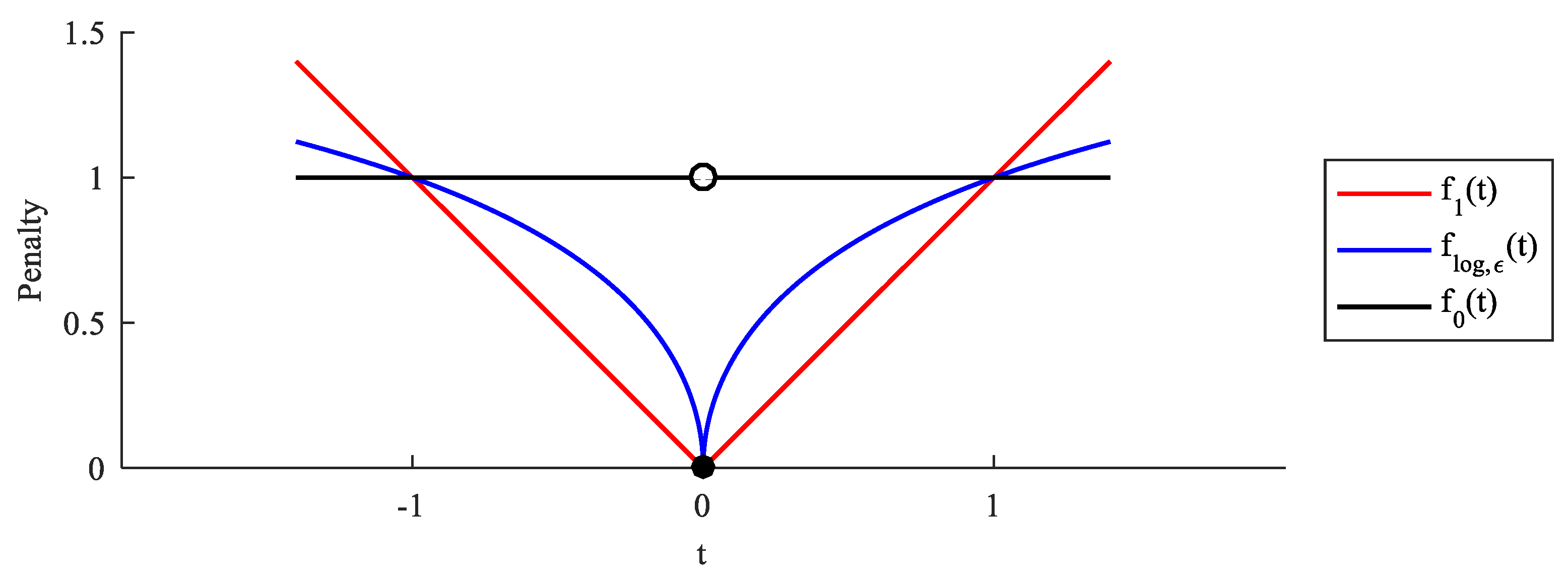
Figure 2.
Plot of thresholding functions. (a) The Hard. (b) The Soft.
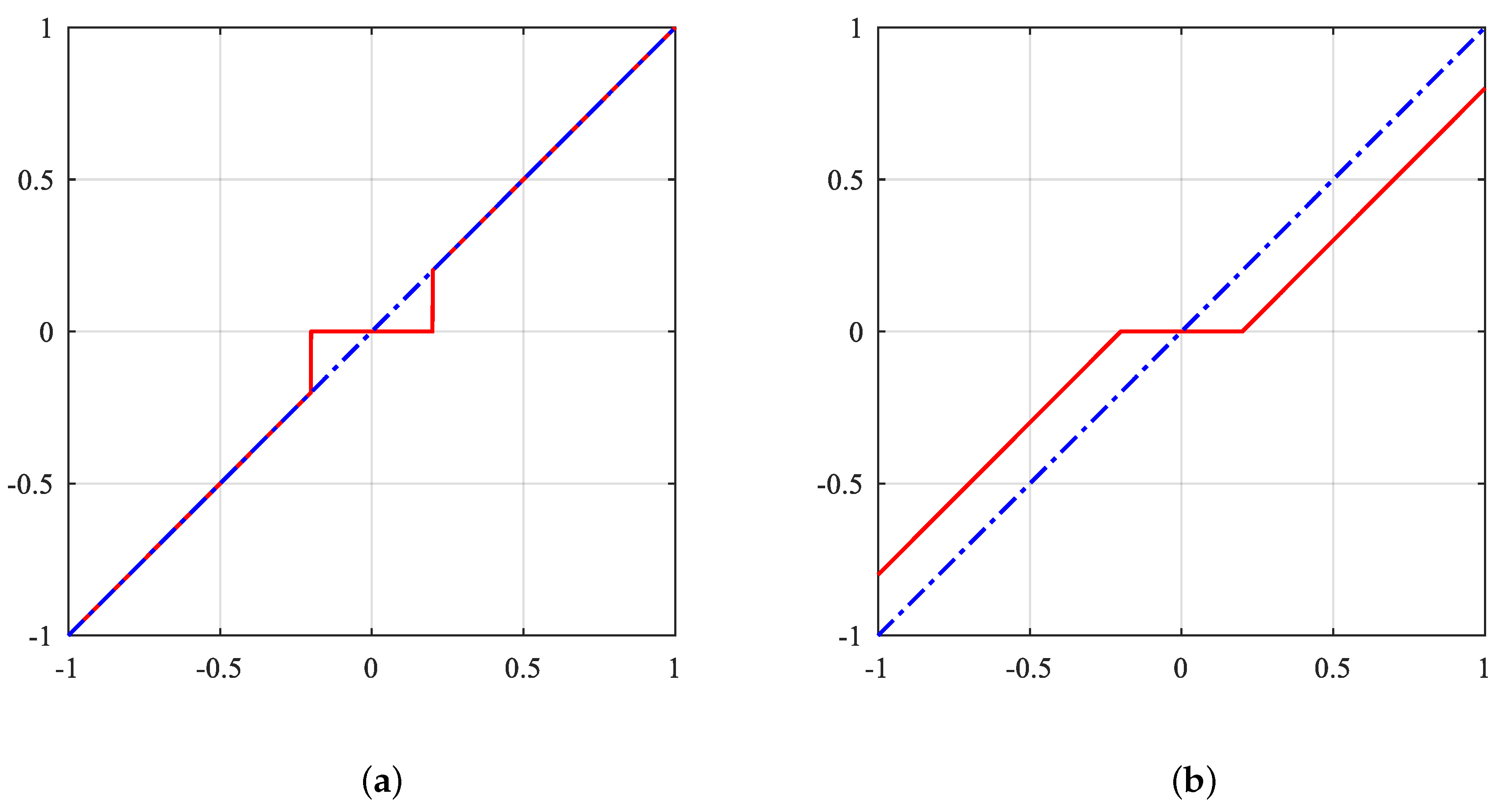
Figure 3.
Plot of thresholding functions. (a) The Half. (b) The Mix. (c) The Firm. (d) The SCAD.
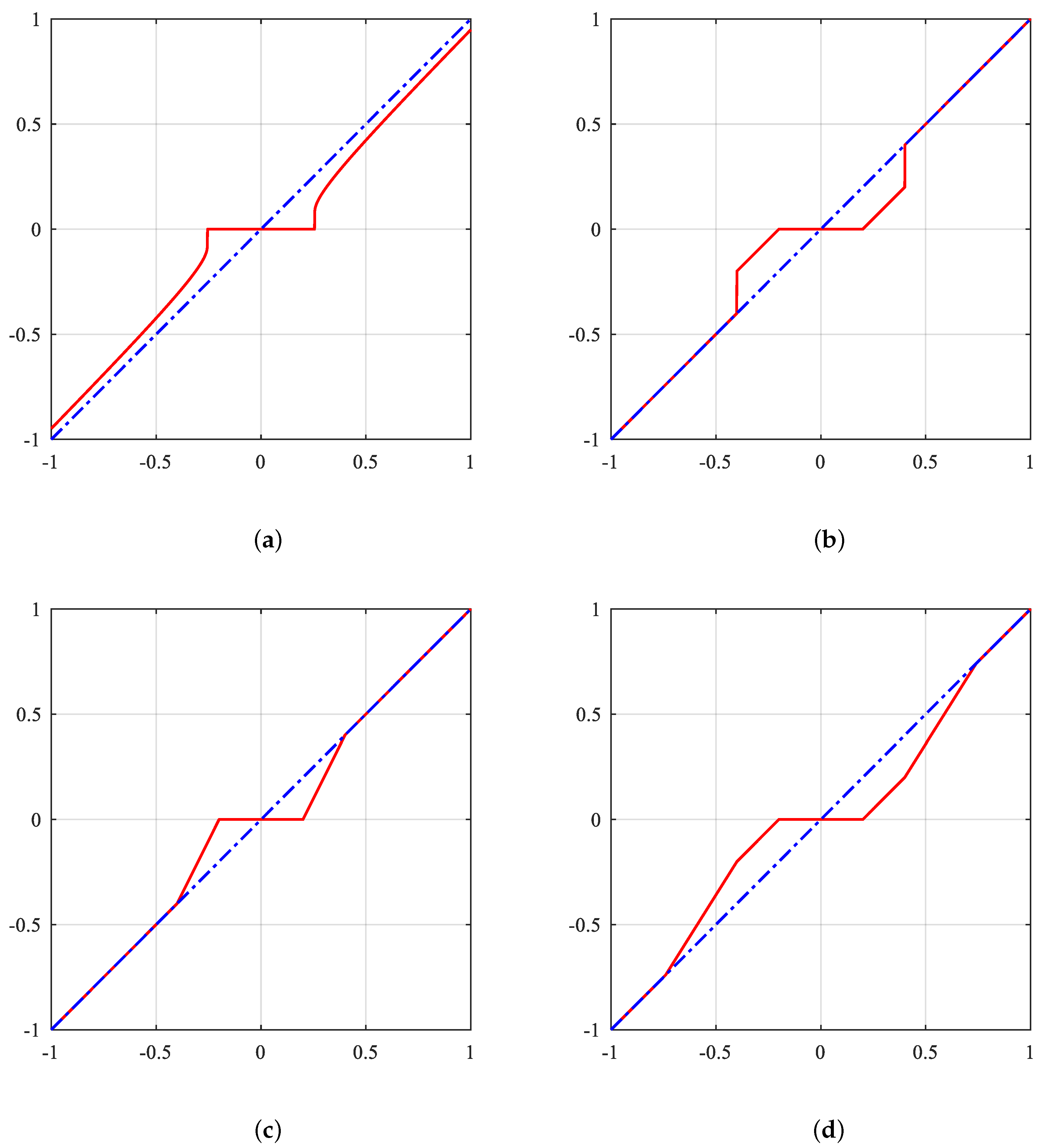
Figure 4.
Sketch maps of amplitude profile with Sinc shaped response and its weighted results. (a) Amplitude profile of two point targets with different RCS. Sinc shaped response is adopted but with only the first two sidelobes are depicted for simplicity. Weighted results with (b) ; (c) in Equation (39); and (d) in Equation (41)..
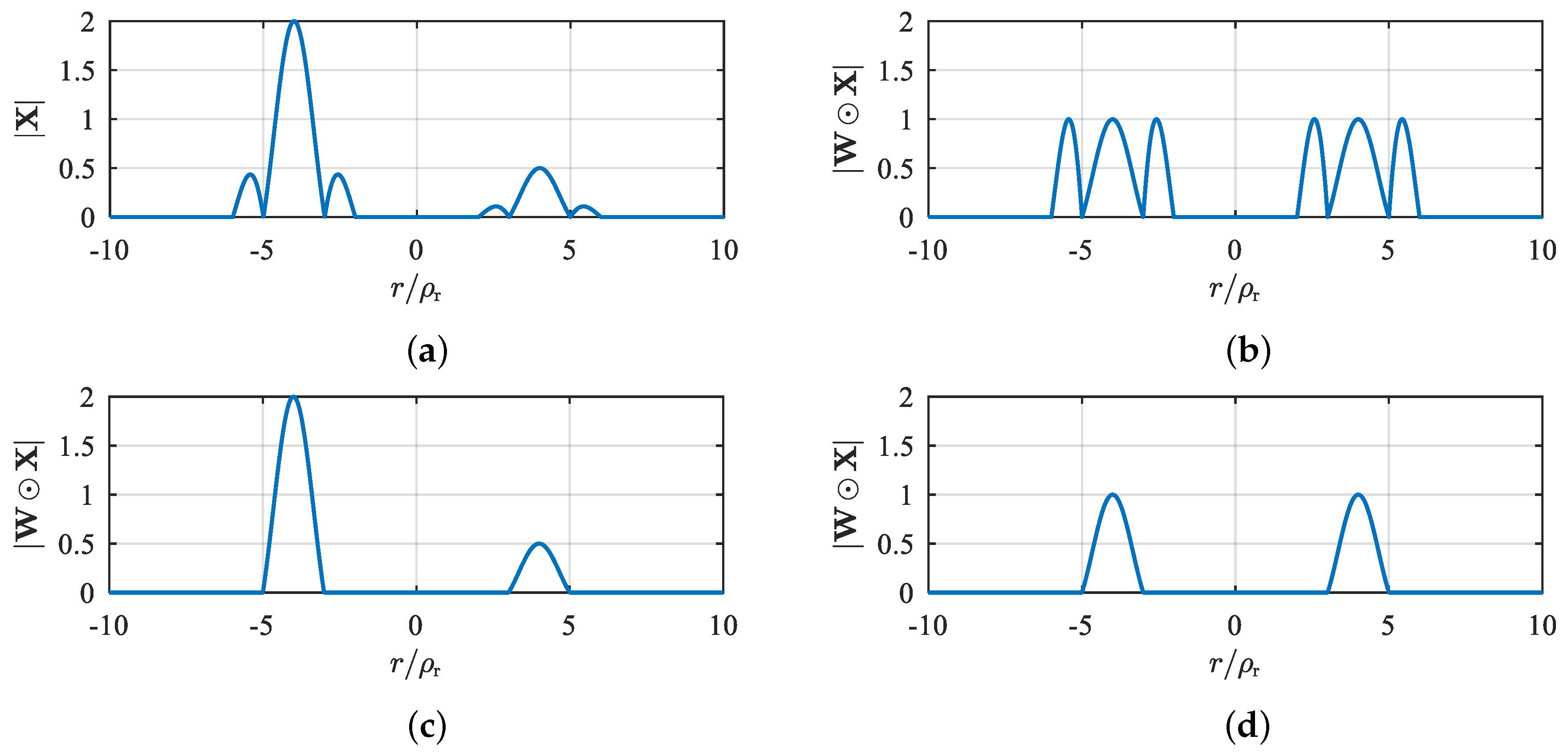
Figure 5.
Plot of TRUTH functions with different numbers of segments P. (a) TRUTH with . (b) TRUTH with . (c) TRUTH with . (d) TRUTH with .
Figure 5.
Plot of TRUTH functions with different numbers of segments P. (a) TRUTH with . (b) TRUTH with . (c) TRUTH with . (d) TRUTH with .
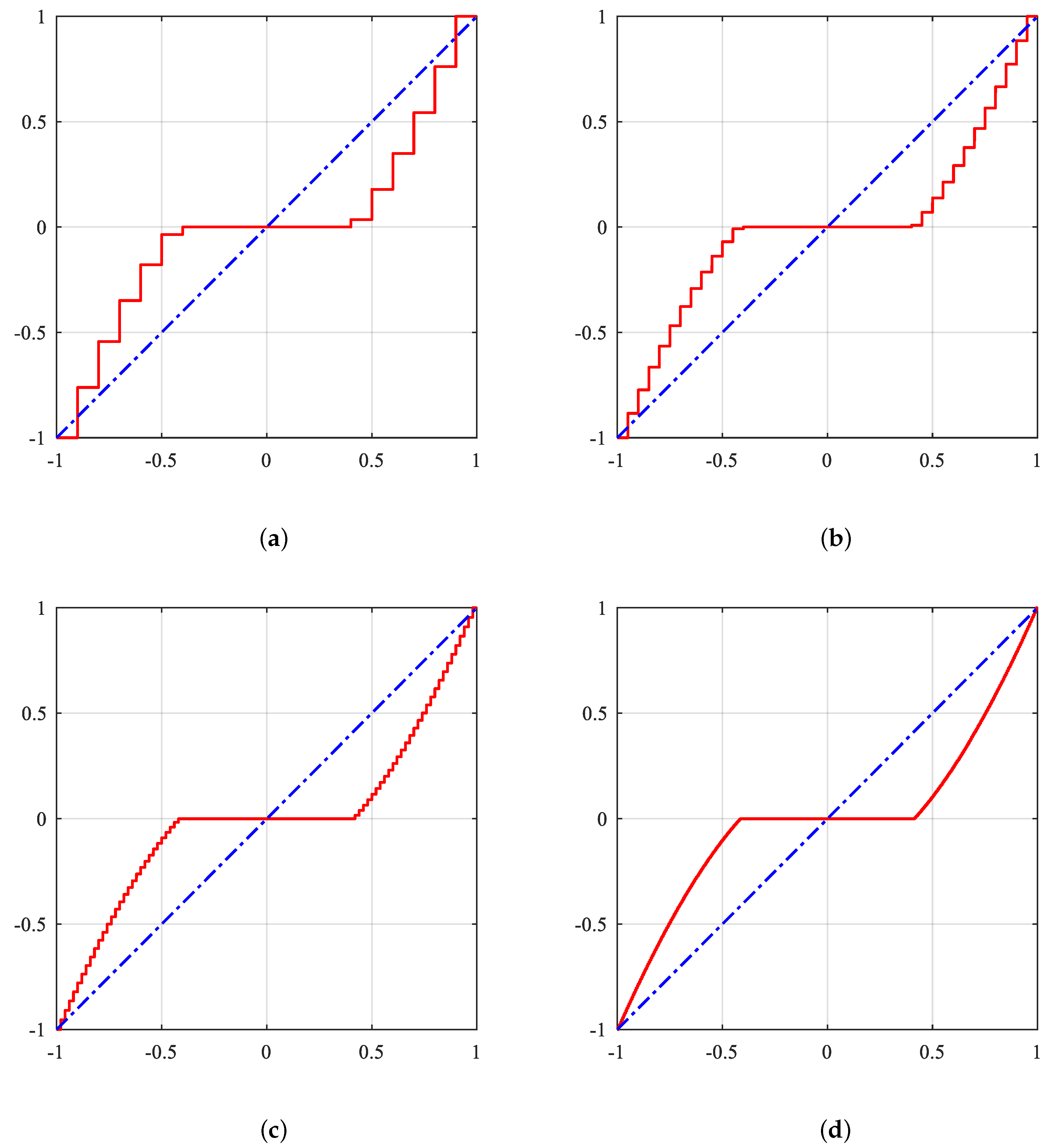
Figure 6.
Plot of TRUTH functions with different super-resolution factors . (a) TRUTH with . (b) TRUTH with . (c) TRUTH with . (d) TRUTH with .
Figure 6.
Plot of TRUTH functions with different super-resolution factors . (a) TRUTH with . (b) TRUTH with . (c) TRUTH with . (d) TRUTH with .
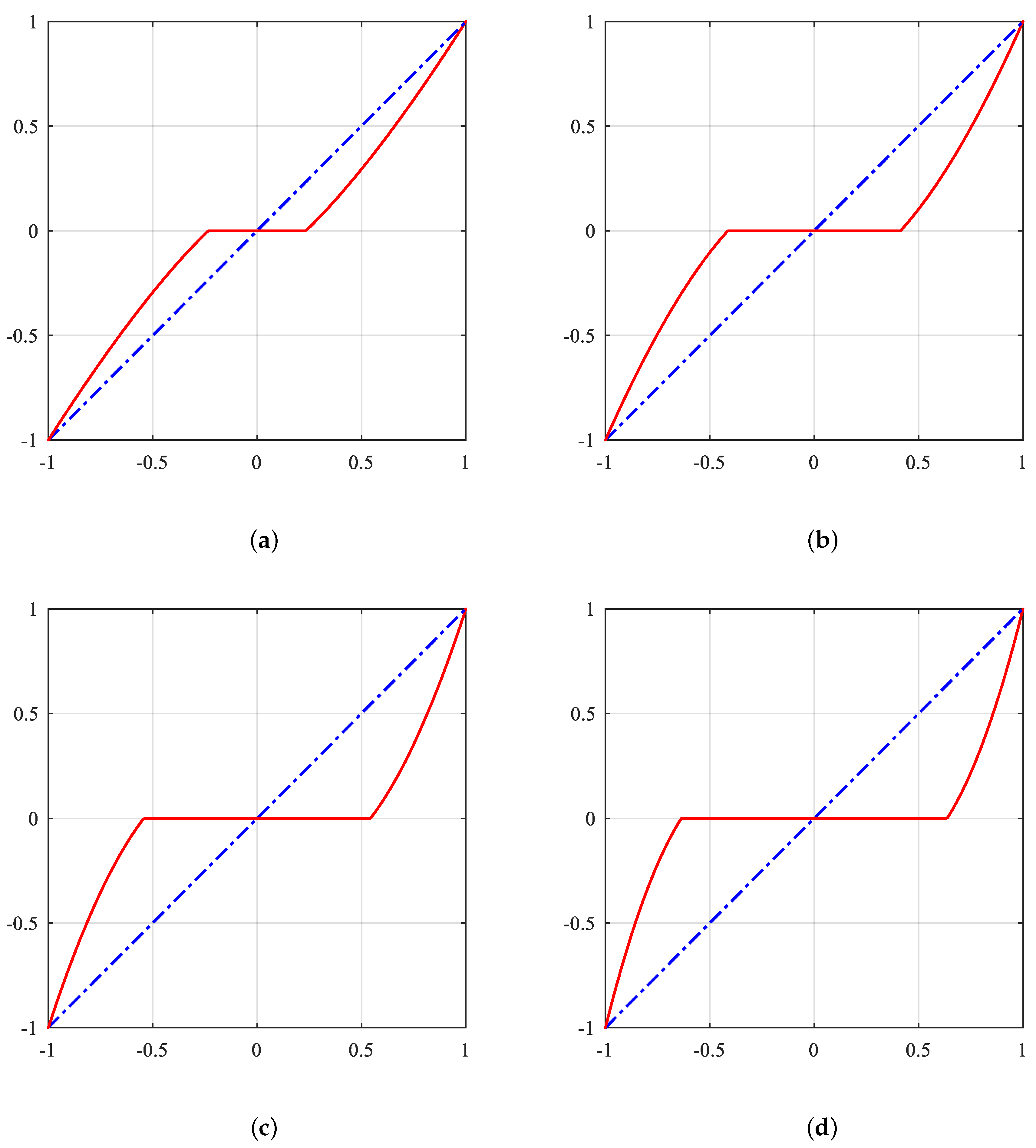
Figure 7.
(a) Illustration of echo acquisition in a parking lot scenario (Top View). (b) The coarsely focused automotive SAR image recovered via RMA. Horizontal axis is range direction, and vertical axis is azimuth direction.
Figure 7.
(a) Illustration of echo acquisition in a parking lot scenario (Top View). (b) The coarsely focused automotive SAR image recovered via RMA. Horizontal axis is range direction, and vertical axis is azimuth direction.
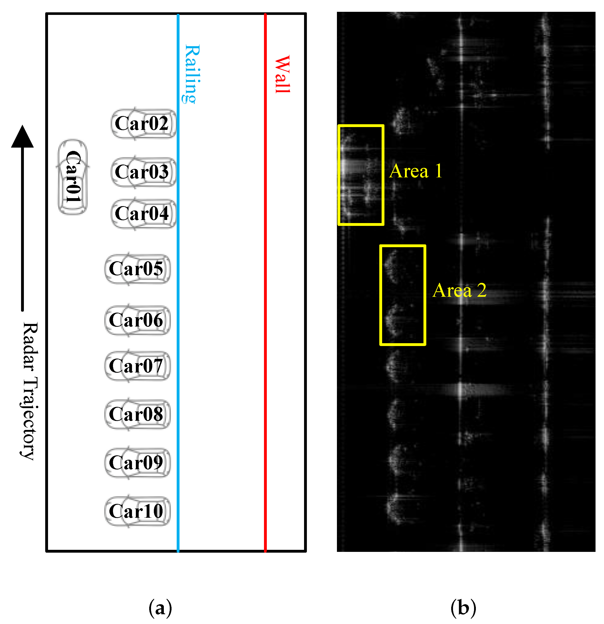
Figure 8.
The L-curve and metrics of norm regularization results with different selected. (a) The black solid line denotes the L-curve with , and the optimal parameter value of is selected at the corner marked as red circle ∘, where . (b) The normalized energy of the highest sidelobe versus different . (c) The number of residual background peaks versus different . (d) The number of reserved target scatters versus different . The red arrow → points to parameter optimization direction.
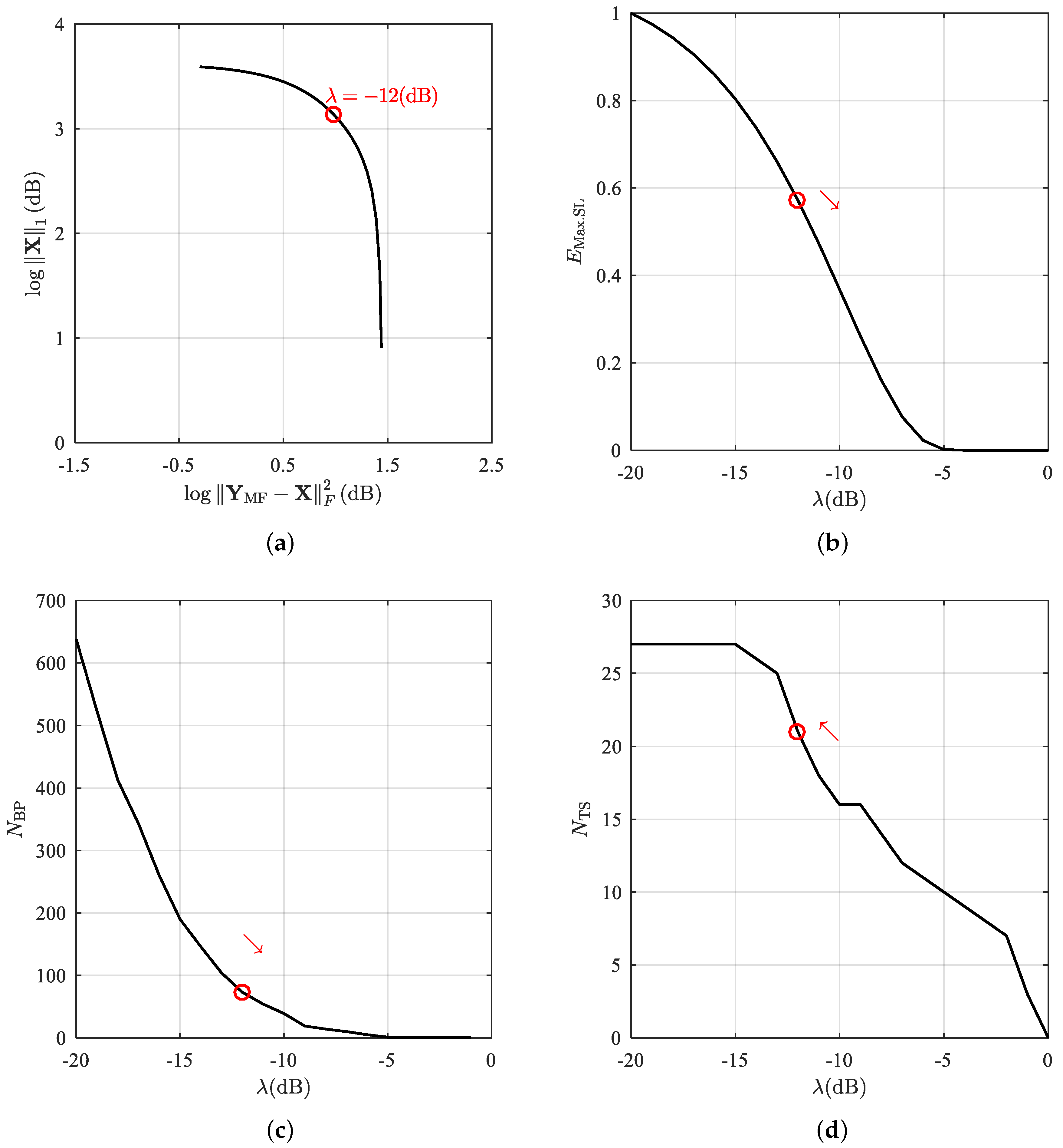
Figure 9.
The local enlarged image of Area1 and its enhanced results via unweighted regularization with different selected. (a) Local enlarged image of Area1 imaged via RMA. (b) Enhanced result of unweighted norm regularization with . (c) and (d) with and respectively.
Figure 9.
The local enlarged image of Area1 and its enhanced results via unweighted regularization with different selected. (a) Local enlarged image of Area1 imaged via RMA. (b) Enhanced result of unweighted norm regularization with . (c) and (d) with and respectively.
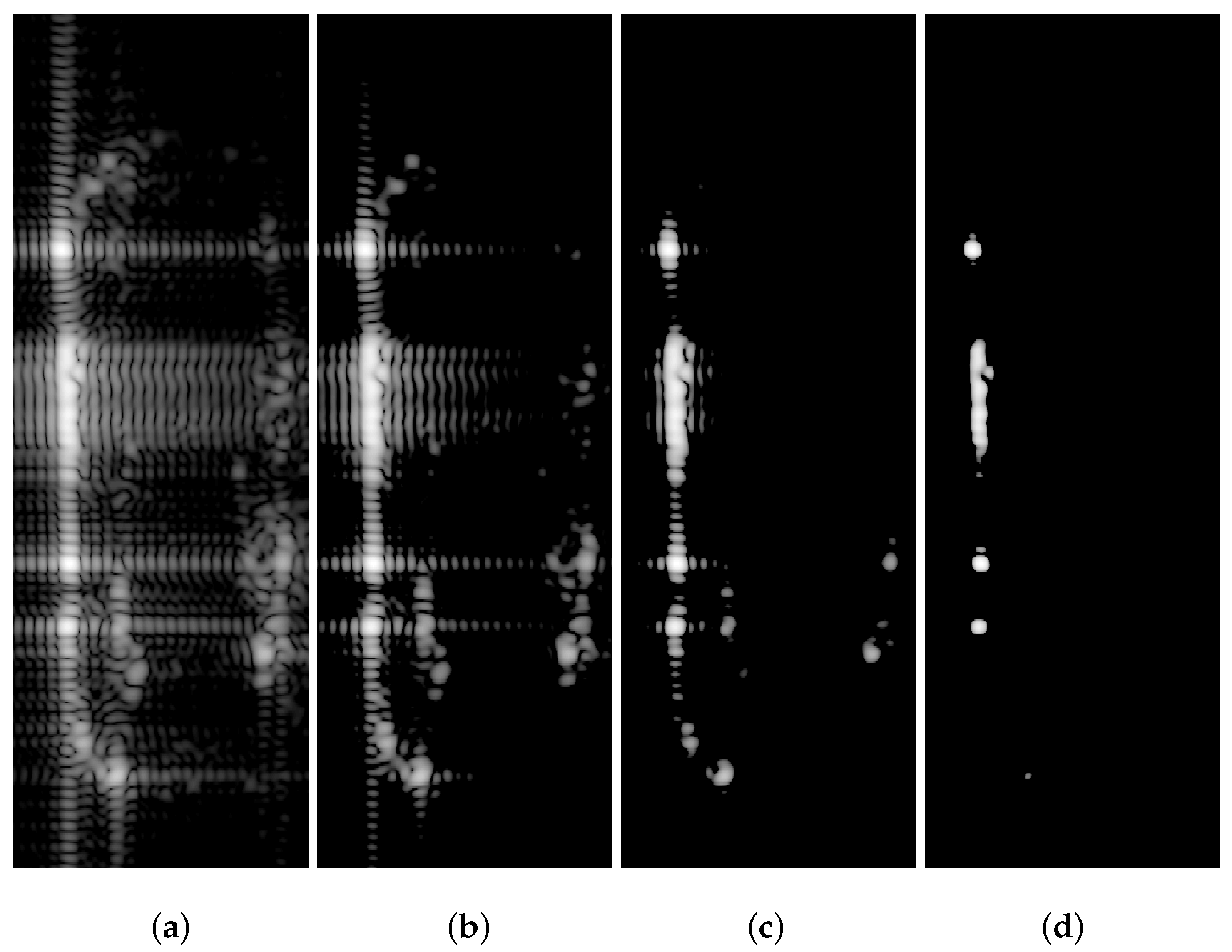
Figure 10.
The enhanced results of Area1 SAR image via (a) SVA, (b) RL1 with weighting scheme WS2, (c) RL1 with weighting scheme WS3, (d) RL1 with weighting scheme WS6, (e) RL1 with weighting scheme WS7 and (b) RL1 with our weighting scheme in Equation (41).
Figure 10.
The enhanced results of Area1 SAR image via (a) SVA, (b) RL1 with weighting scheme WS2, (c) RL1 with weighting scheme WS3, (d) RL1 with weighting scheme WS6, (e) RL1 with weighting scheme WS7 and (b) RL1 with our weighting scheme in Equation (41).
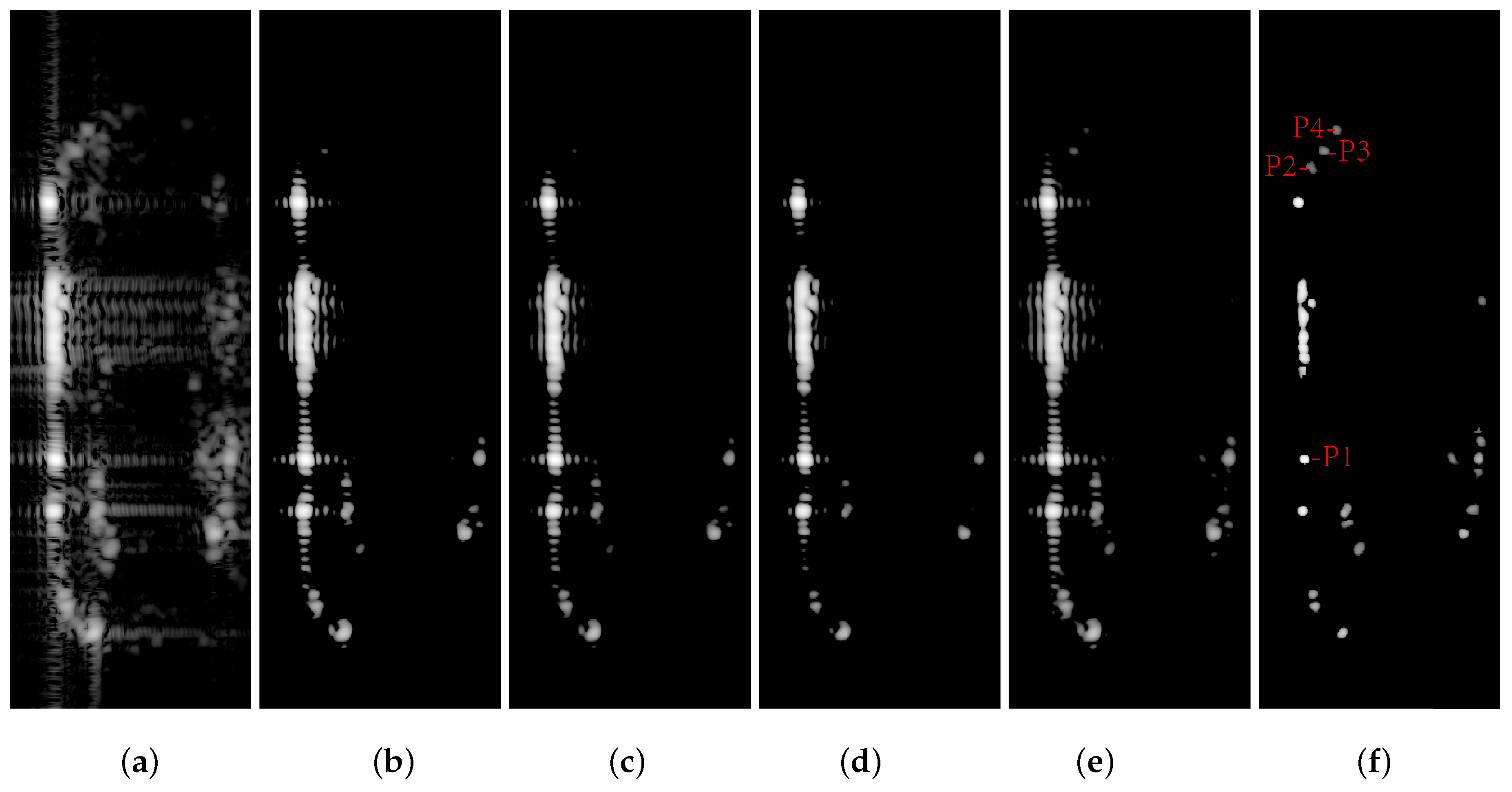
Figure 11.
The local enlarged image of Area2 , the resolution degraded result and resolution re-enhanced results. (a) RMA image with resolution . (b) RMA image with resolution . (c∼f) Enhanced results of MSR with our weighting scheme and . (c) . (d) . (e) . (f) .
Figure 11.
The local enlarged image of Area2 , the resolution degraded result and resolution re-enhanced results. (a) RMA image with resolution . (b) RMA image with resolution . (c∼f) Enhanced results of MSR with our weighting scheme and . (c) . (d) . (e) . (f) .
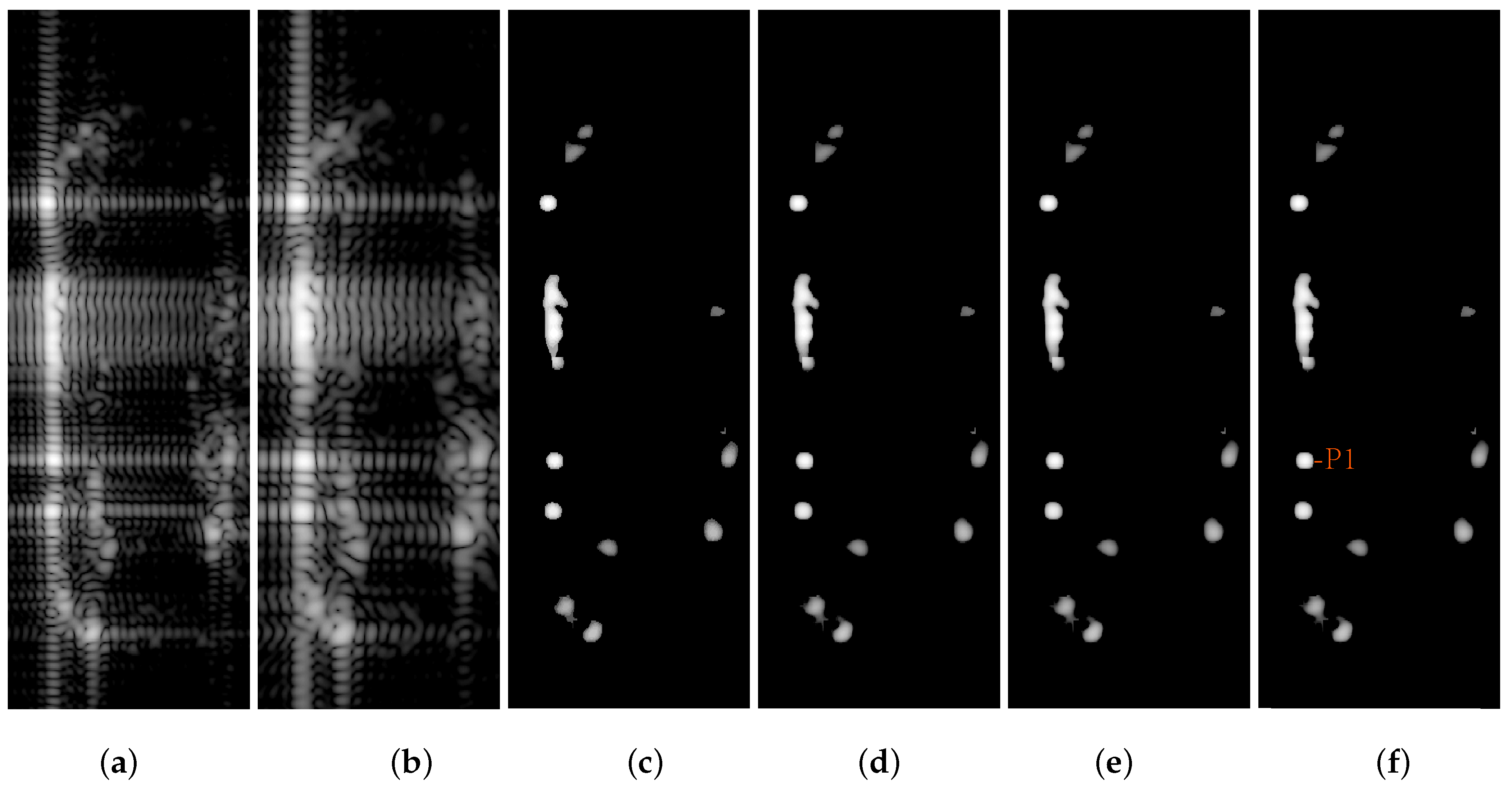
Figure 12.
The contour plots, range profiles, and azimuth profiles of P1 via MSR. The upper row: contour plots. The middle row: range profiles; The lower row: azimuth profiles. The first column: ; The second column: ; The third column: ; The fourth column: . The green line: the profiles of strongest scatters with resolution . The black line: the profiles of strongest scatters with resolution , and the red plus marks +: the enhanced results.
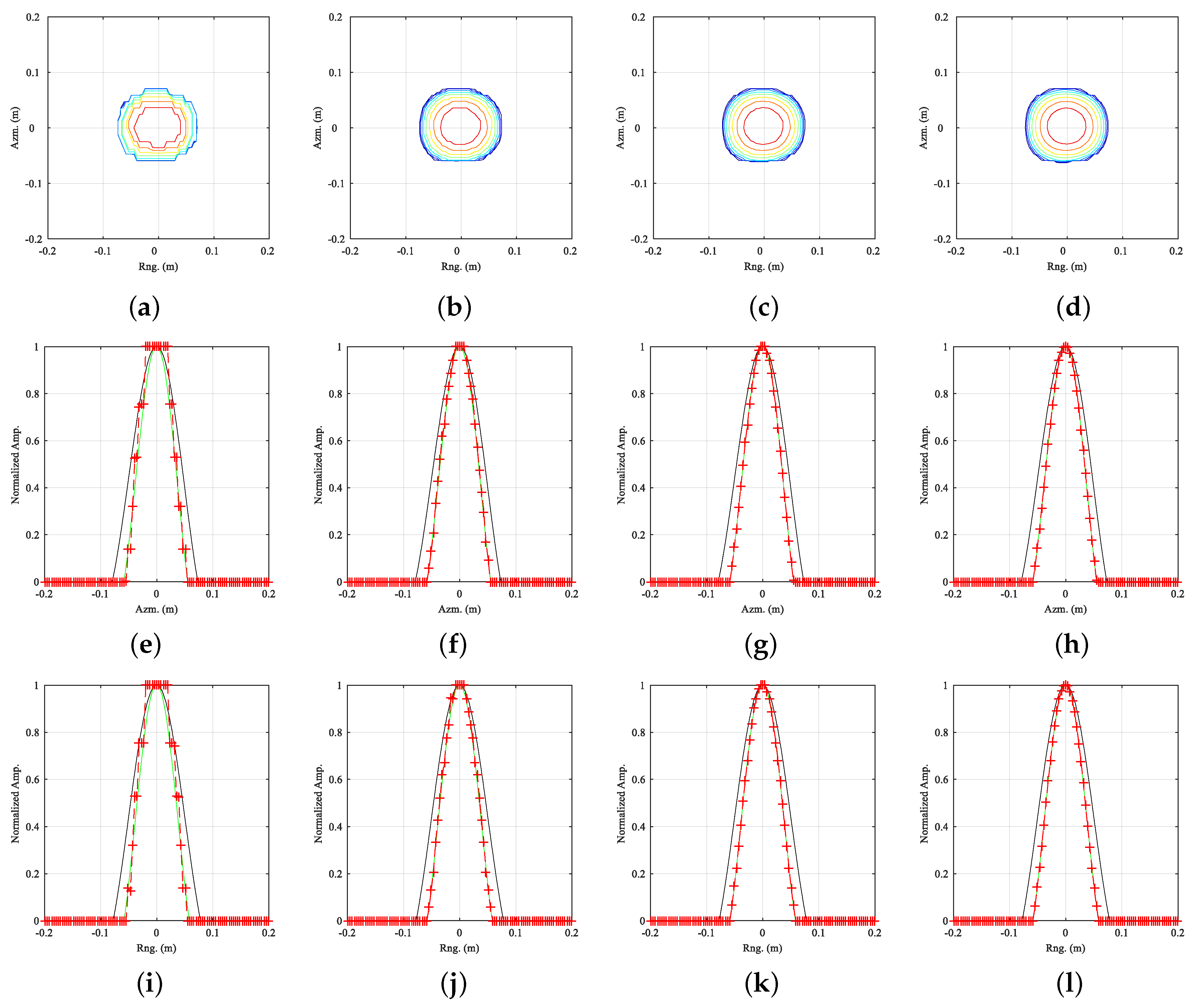
Figure 13.
Metrics of MSR enhancing performance versus segmented number P. (a) RMSE versus P. (b) SSIM versus P.
Figure 13.
Metrics of MSR enhancing performance versus segmented number P. (a) RMSE versus P. (b) SSIM versus P.
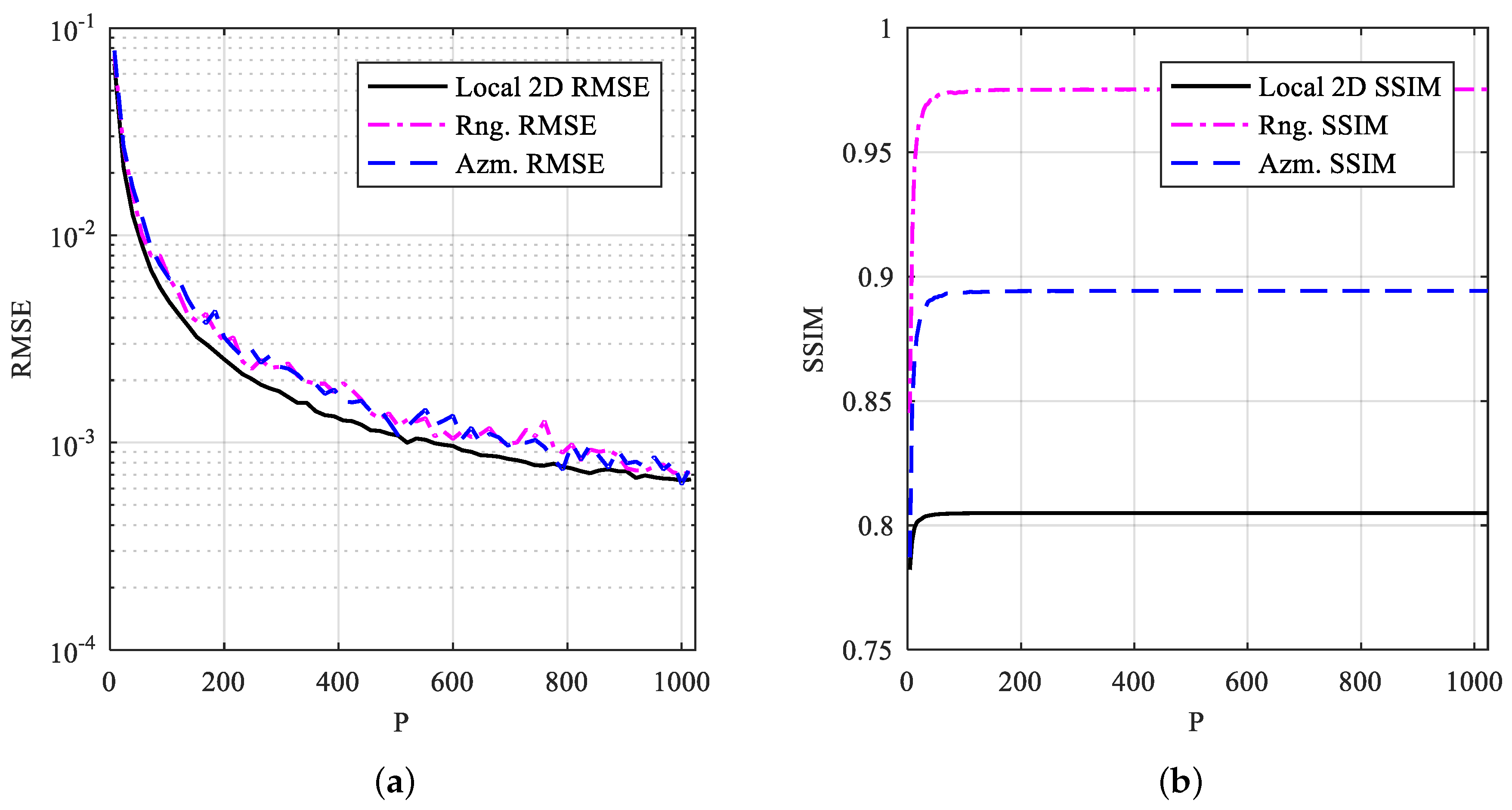
Figure 14.
Azimuth profiles of the point with the strongest amplitude in the enhanced results of MSR with different thresholding functions. (a) The Hard. (b) The Soft. (c) The Half. (d) The Garrote+. (e) The Firm. (f) The Mix. (g) The SCAD. (h) The TRUTH.
Figure 14.
Azimuth profiles of the point with the strongest amplitude in the enhanced results of MSR with different thresholding functions. (a) The Hard. (b) The Soft. (c) The Half. (d) The Garrote+. (e) The Firm. (f) The Mix. (g) The SCAD. (h) The TRUTH.
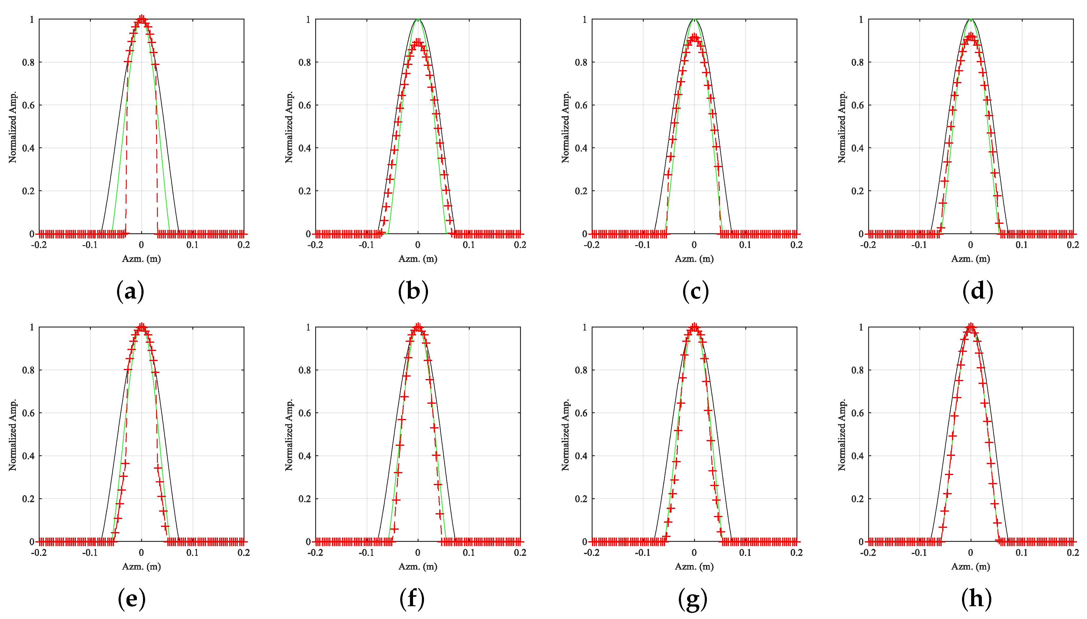
Figure 15.
The same results as Figure 14 but range profiles are shown.
Figure 15.
The same results as Figure 14 but range profiles are shown.
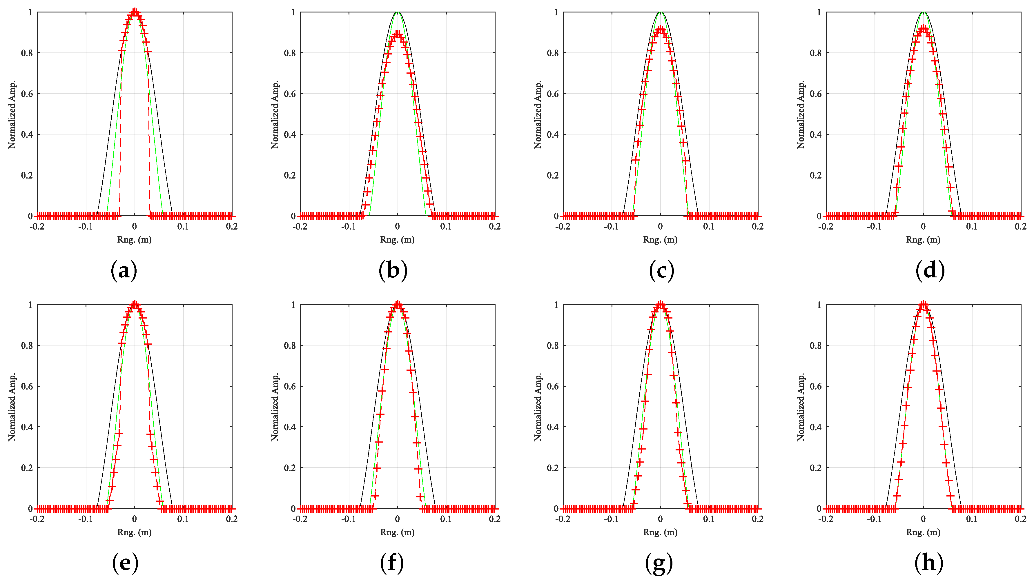
Figure 16.
Local enlarged image of Area2 and its enhanced results. (a) Local enlarged image of Area2 imaged via RMA. (b) Enhanced result of unweighted norm regularization. (c) Enhanced result of RL1 with our weighting scheme. (d) Enhanced result of MSR with our weighting scheme.
Figure 16.
Local enlarged image of Area2 and its enhanced results. (a) Local enlarged image of Area2 imaged via RMA. (b) Enhanced result of unweighted norm regularization. (c) Enhanced result of RL1 with our weighting scheme. (d) Enhanced result of MSR with our weighting scheme.
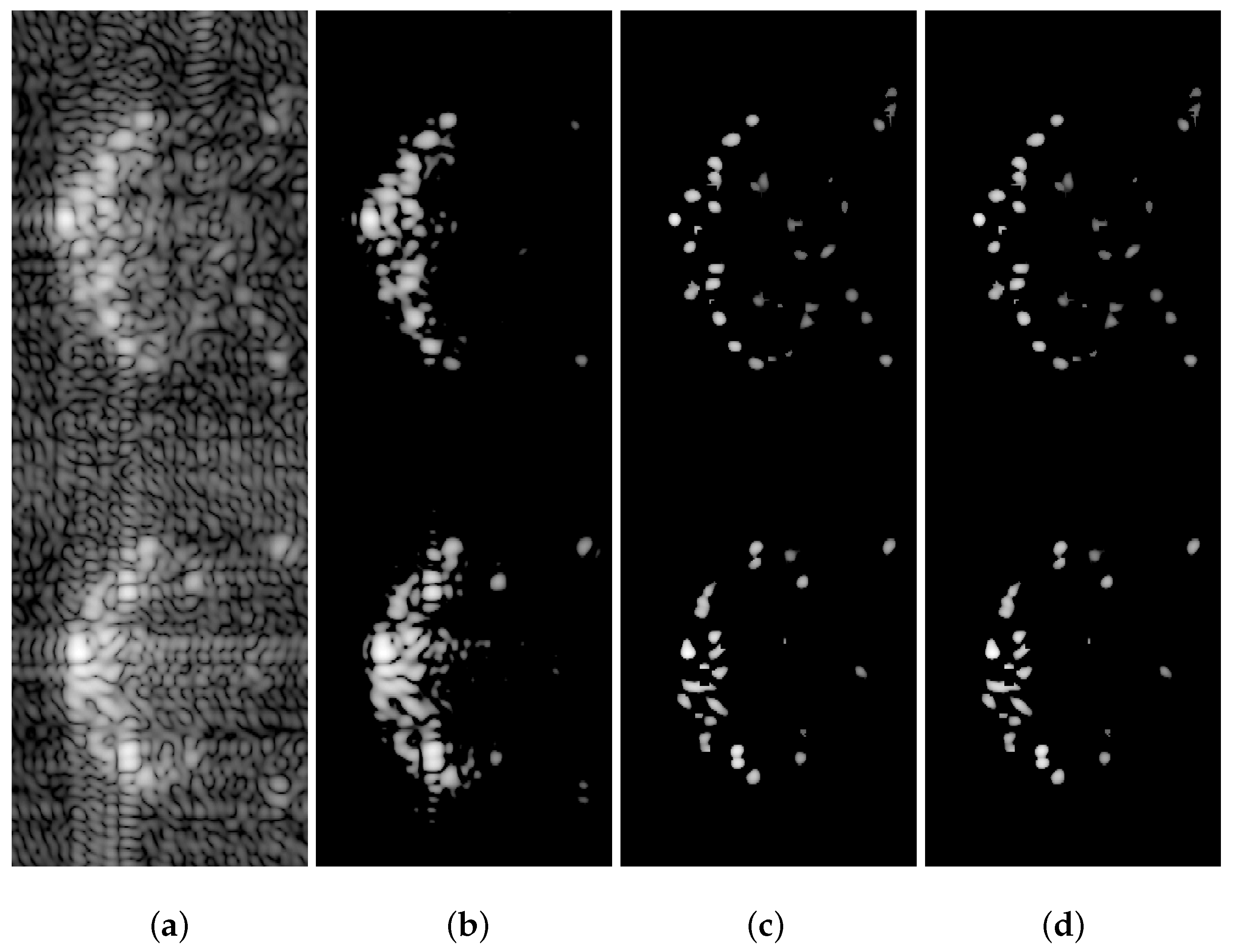
Figure 17.
The selected scattering points and their amplitude bias after being enhanced. (a) The 76 selected scattering points form Area2. (b) The estimated amplitudes versus the true amplitudes after being enhanced via unweighted norm regularization. Similarly, (c) and (d) are respectively via RL1 and MSR with our weighting scheme. The blue diagonal lines mean unbiased reference line.
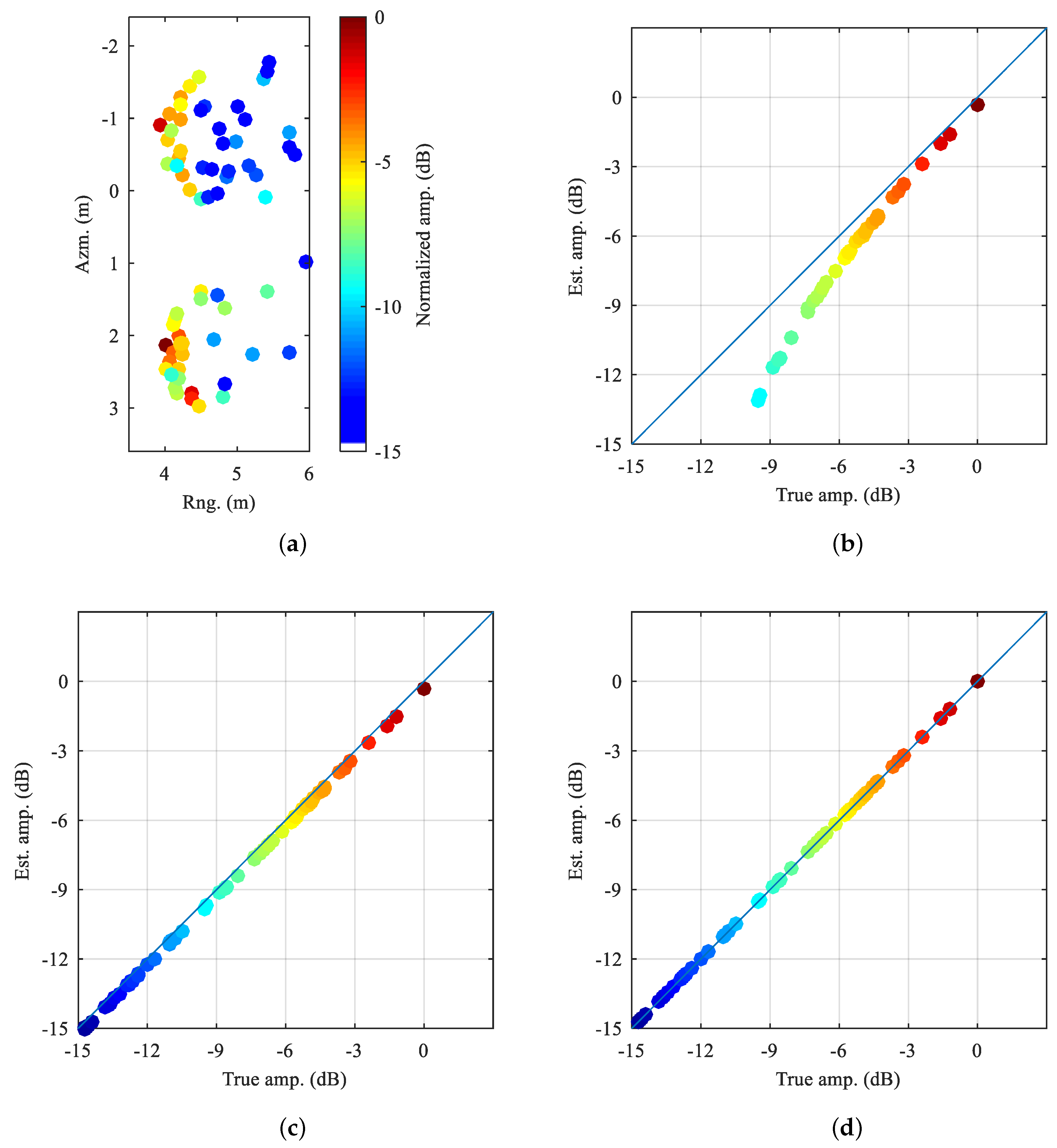
Figure 18.
3dB mainlobe resolutions of the selected 76 scattering points and resolution enhancing analysis. (a) 3dB mainlobe resolutions of the selected 76 scattering points form Area2 RMA image. (b) 3dB mainlobe resolutions after being enhanced via unweighted norm regularization. Similarly, (c) and (d) are respectively via RL1 and MSR with our weighting scheme. The red ellipses with parameter are radiational transformed from the one with .
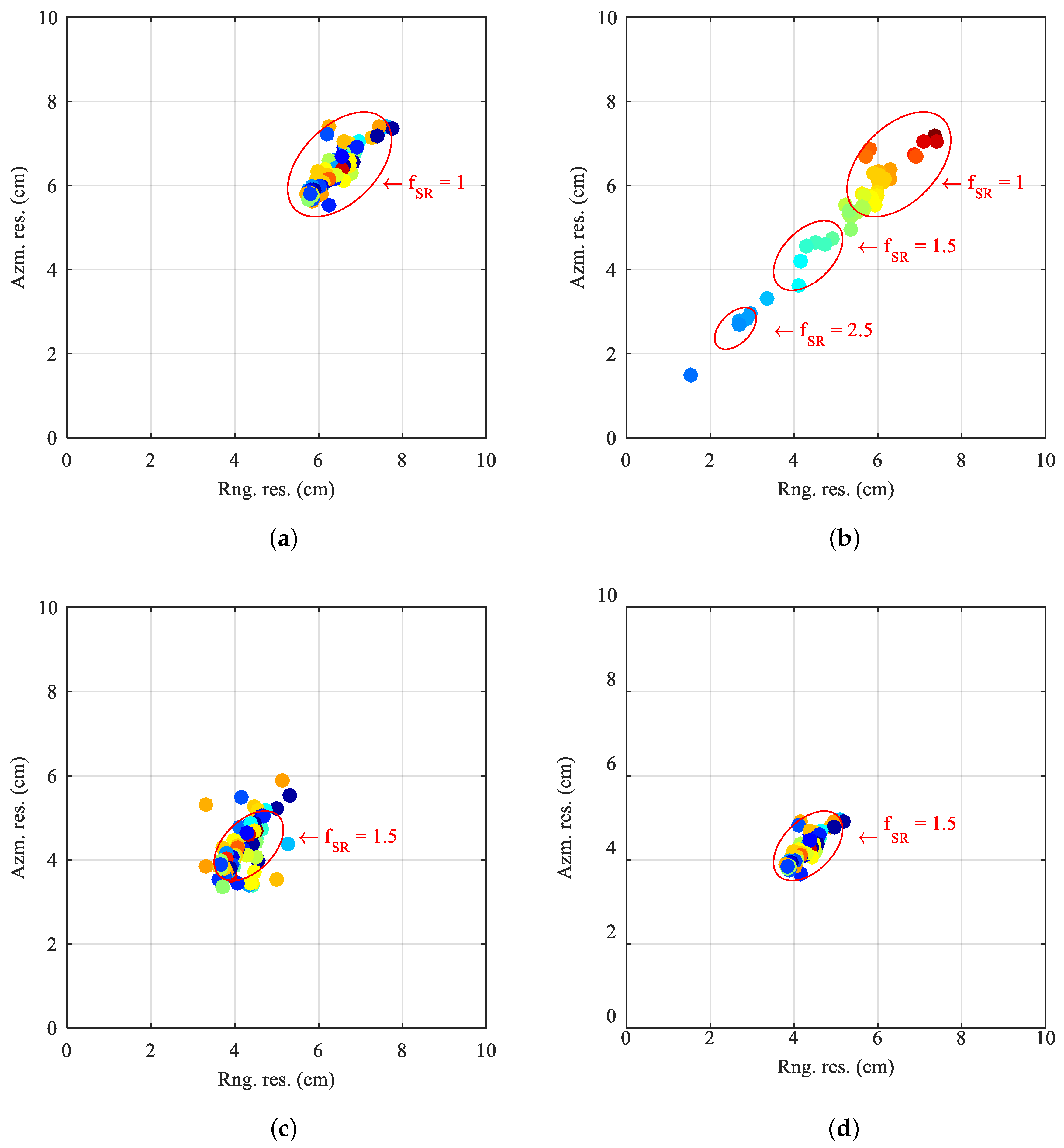

Table 1.
weighting schemes and their equivalent penalty problems, together with their related adaptive lasso forms.
Table 1.
weighting schemes and their equivalent penalty problems, together with their related adaptive lasso forms.
| Optimization Methods | Reweighting Norm | Equivalent Penalty | Adaptive Lasso * |
|---|---|---|---|
| Problem Formula | |||
| Weighting Scheme 1(WS1) | (When allowed to expand) | ||
| Weighting Scheme 2(WS2) | (When allowed to be neglected) | ||
| Weighting Scheme 3(WS3) | (When allowed to be neglected) | ||
| Weighting Scheme 4(WS4) | (When allowed to be neglected) | ||
| Weighting Scheme 5(WS5) | (When allowed to be neglected) | ||
| Weighting Scheme 6(WS6) | (When allowed to be neglected) |
* The adaptive lasso is not equivalent to the weighting scheme or the penalty problem in the same row of the table, but it can be regarded as as a special case when the parameters meet specific conditions. The conditions are listed in brackets.
Table 2.
Metrics of RL1 automotive SAR image enhanced results with different weighting schemes.
| Method | RMA | SVA | WS1 | WS2 | WS3 | WS6 | WS7 | Ours |
|---|---|---|---|---|---|---|---|---|
| Figure label | Figure 9(a) | Figure 10(a) | Figure 9(c) | Figure 10(b) | Figure 10(c) | Figure 10(d) | Figure 10(e) | Figure 10(f) |
| IE | 5.22* | 3.85 | 0.54 | 0.61 | 0.61 | 0.42 | 0.78 | 0.20* |
| IC | 1.32 | 1.83 | 5.50 | 5.19 | 5.01 | 6.34 | 4.53 | 9.35 |
| ENL | 9.41E-2 | 5.30E-2 | 1.48E-2 | 1.59E-2 | 1.84E-2 | 1.23E-2 | 1.85E-2 | 5.60E-3 |
| RaRes(dB) | 6.29 | 7.28 | 9.64 | 9.51 | 9.23 | 10.01 | 9.21 | 11.56 |
| TBR(dB) | 7.86 | 9.24 | 13.64 | 13.20 | 11.71 | 15.23 | 12.37 | Inf |
| 638 | 237 | 73 | 86 | 93 | 54 | 104 | 0 | |
| 27 | 27 | 21 | 23 | 23 | 18 | 24 | 27 | |
| (dB) | -13.50 | -22.30 | -19.52 | -18.77 | -16.33 | -22.57 | -17.22 | -Inf |
| (dB) | -7.34 | -10.31 | -9.71 | -9.45 | -8.17 | -10.98 | -9.26 | -Inf |
| (dB) | -15.47 | -20.38 | -18.99 | -18.53 | -16.52 | -21.19 | -17.58 | -Inf |
| (dB) | -8.92 | -11.19 | -10.03 | -9.91 | -9.12 | -10.85 | -9.96 | -Inf |
* The red and the blue numbers denote the worst and the best performance metrics respectively within the current row of values.
Table 3.
Metrics of MSR automotive SAR image enhancing with different different thresholding functions.
Table 3.
Metrics of MSR automotive SAR image enhancing with different different thresholding functions.
| Threshold | Hard | Soft | Half | Garrote+ | Firm | Mix | SCAD | TRUTH |
|---|---|---|---|---|---|---|---|---|
| Peak Bias(dB) | 0* | 0.49* | 0.38 | 0.36 | 0 | 0 | 0 | 0 |
| Local 2D RMSE | 0.2437 | 0.1572 | 0.0898 | 0.0788 | 0.0885 | 0.1174 | 0.0639 | 0.0011 |
| Rng. RMSE | 0.0885 | 0.0671 | 0.0534 | 0.0503 | 0.0509 | 0.0620 | 0.0453 | 0.0015 |
| Azm. RMSE | 0.0881 | 0.0643 | 0.0524 | 0.0492 | 0.0493 | 0.0614 | 0.0445 | 0.0014 |
| Local 2D SSIM | 0.7775 | 0.7750 | 0.7949 | 0.7983 | 0.7904 | 0.7908 | 0.7994 | 0.8050 |
| Rng. SSIM | 0.8312 | 0.8662 | 0.9264 | 0.9427 | 0.9096 | 0.8990 | 0.9476 | 0.9753 |
| Azm. SSIM | 0.7713 | 0.8088 | 0.8636 | 0.8684 | 0.8417 | 0.8304 | 0.8719 | 0.8943 |
* The red and the blue numbers denote the worst and the best performance metrics respectively within the current row of values.
Disclaimer/Publisher’s Note: The statements, opinions and data contained in all publications are solely those of the individual author(s) and contributor(s) and not of MDPI and/or the editor(s). MDPI and/or the editor(s) disclaim responsibility for any injury to people or property resulting from any ideas, methods, instructions or products referred to in the content. |
© 2025 by the authors. Licensee MDPI, Basel, Switzerland. This article is an open access article distributed under the terms and conditions of the Creative Commons Attribution (CC BY) license (http://creativecommons.org/licenses/by/4.0/).
Copyright: This open access article is published under a Creative Commons CC BY 4.0 license, which permit the free download, distribution, and reuse, provided that the author and preprint are cited in any reuse.


