Submitted:
28 February 2025
Posted:
03 March 2025
You are already at the latest version
Abstract
Light Detection and Ranging (LiDAR) technology can be used to assess canopy height in cotton (Gossypium hirsutum L.), but standardized data acquisition and processing guidelines are lacking. Accurate canopy height estimation is crucial in cotton for optimizing growth regulator application and maximizing yield. The main goal of this study was to determine the optimal unmanned aerial vehicle flight settings—altitude and speed—and to assess specific processing parameters impact on data accuracy, processing time, and file size. Nine flight settings comprising three altitudes (12.2 m, 24.4 m, and 48.8 m) and three speeds (4.8 km/h, 9.6 km/h, and 14.8 km/h) were tested. LiDAR data were processed using DJI Terra software, where two user-defined processing steps were examined: point-cloud thinning via grid size sub-sampling (0, 10, 20, 30, 40, and 50 cm) and slope classification (flat, gentle, and steep). The optimal flight altitude was 24.4 m, with no effect of flight speed. Grid sub-sampling up to 20 cm produced balanced accuracy, processing time, and file size. The choice of slope category had no significant effect on LiDAR-derived canopy height. These findings contribute to the development of standardized LiDAR data acquisition and processing guidelines for cotton to support crop management decision.
Keywords:
point cloud
; LAS
; DTM
; DSM
; CHM
; TIN
1. Introduction
Cotton (Gossypium hirsutum L.) is one of the most significant fiber crops globally. The U.S. produced around 14.4 million bales of cotton in the year 2023/24, ranking forth globally in cotton production after India, China and Brazil [1]. Within the U.S., Texas (30%), Georgia (16%), and Arkansas (9%) are the largest cotton producing states, responsible for 55% of cotton lint production in the U.S. and 12% of world production [2].
Cotton is a perennial plant that is cultivated as an annual crop. This is achieved by using management techniques such as plant growth regulators, which help control growth rate and plant height, preventing the crop from expending too much energy on vegetative growth and directing it towards reproductive growth [3,4]. Balancing vegetative and reproductive sinks is important in cotton to optimize fiber yield and quality [5].
Different metrics exist to determine cotton growth rates and serve as a decision-making tools for deciding the timing and rate of synthetic plant growth regulator applications [6]. The most commonly used metrics are the height-to-node ratio (HNR) (ratio between plant height and total number of nodes) and length of the upper five internodes [7]. HNR values below growth-stage specific thresholds indicate sub-optimal growth rates, whereas values above the threshold indicate excessive growth rates that need to be controlled using exogenously applied plant growth regulators like mepiquat chloride. For example, during the early bloom stage, if the HNR exceeds 6.4 cm/node, it is recommended to apply mepiquat chloride at a rate ranging from 0.5 to 2 L/ha at a standard concentration of 4.2% w/v [8]. The rate of application is determined based on multiple factors, including the cotton variety, the plant growth stage, the current rate of vegetative growth and weather conditions [8,9] .
Traditionally, plant height is determined by visiting the field and collection manual height measurements on plants across multiple areas in the field. This approach is time and labor intensive, and as cotton plants grow and form dense canopies, walking a field can potentially damage the crop. For large-scale commercial farming, such manual methods are impractical for achieving the required precision and speed in decision-making. Additionally, capturing height variation accurately across large fields remains one of the biggest constraints, as it directly impacts yield estimation, canopy structure analysis, and variable rate input applications.
To overcome this issue, different technologies have been developed to create estimated continuous maps of plant height, including unmanned aerial vehicle (UAV) imagery-based canopy height model (difference of the height at the top of the plant canopy and the elevation of the bare ground) [10,11]; tractor mounted LiDAR (Light Detection and Ranging) [12]; and UAV-based LiDAR systems. The latter has emerged as a solution to bridge the gap between ground-based platforms, known for their high accuracy but low efficiency, and UAV imagery-based platforms, which offer extensive coverage but limited detail [13]. Moreover, LiDAR directly measures crop height by emitting laser pulses, making it more accurate than UAV-mounted passive spectral imaging, which relies on ambient light and requires additional processing [14]. Height estimation from spectral data depends on photogrammetry techniques like structure-from-motion (SfM), which reconstructs 3D models based on overlapping images [15]. This approach requires ideal lighting, minimal occlusion, and accurate tie points, with additional steps to separate crop height from ground elevation. Errors in shadowed areas, vegetation movement, or point matching can reduce accuracy, making LiDAR the more reliable option for precise height measurements, especially in dense or complex canopies [16].
LiDAR's application in row crops such as maize started around the mid-2010s, when it was used for evaluating crop structure [17] and predicting yield potential [18]. Studies on the use of UAV-mounted LiDAR to estimate plant height in cotton are scant [19].This is a limitation especially because different flight settings like altitude and speed, and data processing steps like point cloud classification, grid size for height extraction and canopy modelling, can contribute to the accuracy of LiDAR-based height estimates, yet no studies exist that provide best-practice recommendations for the cotton crop.
For example, adjusting the point cloud density—the number of laser returns per square meter—is key [20] to generate accurate LiDAR-based height estimates. Achieving a high point cloud density enhances measurement accuracy but requires UAVs to fly at lower altitudes, slower speeds, or with greater overlap between flight paths, all of which extend flight time and increase the cost and complexity of data collection and data processing. High point cloud density poses a challenge as it generates larger data files [21], which demand significant storage capacity and increase computing power requirements and/or processing times. Therefore, identifying flight characteristics and data processing steps that optimize crop height estimation accuracy while minimizing flight time and data storage and processing requirements is of utmost importance.
Another key processing step with LiDAR data is grid-based sub-sampling, where the raw LiDAR point cloud data is selectively thinned based on the highest-height point within each predefined grid cell. By identifying a grid cell size that balances data retention and reduction, we can minimize file size, reduce computational requirements, and improve processing speed, all of which contribute to more efficient and cost-effective UAV-based LiDAR applications. The decision on the size of the grid cell to be utilized at this step is left to the user, and no best-practice recommendations exist when using LiDAR in row crops in general, or cotton in specific.
Another important step when processing LiDAR data in DJI Terra, a LiDAR mapping and analysis software developed by DJI, is selecting the appropriate field slope type for the initial classification of point clouds. This choice helps the software distinguish between ground, and non-ground points based on terrain variation. The classification process is influenced by the field slope characteristics, as variations in topography affect the differentiation between ground and non-ground points. Like grid cell size selection, the decision on the slope choice is left to the user, and no best-practice recommendations exist.
The overall aim of this study was to establish best-practice guidelines for UAV LiDAR flight settings and data processing to ensure high-quality data acquisition for accurate cotton canopy height estimation. The first objective of this study was to determine and select the optimal UAV flight settings—altitude and speed—that provide the most accurate LiDAR-derived crop height estimates. Based on the best flight settings identified in the first objective, the second and third objectives focused on evaluating the impact of two user-dependent data processing steps on crop height estimation. Specifically, the second objective assessed how defining different grid cell size for sub-sampling point clouds affects crop height accuracy, processing time, and file size. The third objective examined the effect of selecting the field slope type on the accuracy of crop height estimation.
2. Materials and Methods
2.1. Experimental site description:
This experiment was conducted in two different irrigated fields in Georgia, USA near Midville (32.875761, -82.222197) and Watkinsville (33.870858, -83.452716) for the year 2024. The field in Midville had a flat terrain predominately characterized by Tifton soil series and the Dothan soil series (Fine-loamy, kaolinitic, thermic plinthic kandiudults), which are both deep, well-drained, and have a fine-loamy texture [22]. The field in Watkinsville has a somewhat flat terrain characterized by Cecil sandy loam soil with 2% to 6% slope [22]. Cotton was planted at a row spacing of 91 cm and seeding rate of 90,000 seeds/ha. The varieties planted were NexGen 3195 Bollgard® 3 XtendFlex® in Watkinsville and Dyna-Gro 3799 Bollgard® 3 XtendFlex® in Midville and were selected according to local recommendations. Planting occurred on 26th of June in Midville and 2nd of July in Watkinsville.
Each trial was implemented as a N fertilizer side-dress rate study, with N rate treatments of 0+0, 112+0, 40+26, 40+60, 40+94, and 40+128 kg/ha, denoted as preplant+side-dress applications. The experiment followed a randomized complete block design with four blocks. In brief, all plots, except for the control (0+0) and the 112+0 treatment, received a baseline application of 40 kg N/ha at planting, applied using a tractor-mounted boom sprayer. The fertilizer source for the application was urea ammonium nitrate (UAN) 28% N, which is a liquid fertilizer. At the blooming crop stage (approximately 49-52 days after planting), side-dress N fertilizer treatments were applied with a variable rate applicator. For this manuscript, the treatment design of N rates was utilized only to generate variability in crop height, and therefore further statistical analysis did not incorporate N rate as an explanatory variable.
2.2 Aerial LiDAR Data Collection and Pre-processing
The workflow for data acquisition, pre-processing, and analysis consisted of four main steps: i) field characterization, ii) data acquisition with different flight settings, iii) data processing, and iv) validation (Figure 1). Field characterization in relation to slope is an important initial step used to define processing settings in the DJI Terra software (DJI, China). DJI Terra provides the user with the option of identifying the field as flat (1-4 degrees slope), gentle (4-7 degrees slope), or steep (8-12 degrees slope) as one of the first steps in the processing pipeline. To conduct field characterization in our study, elevation data were retrieved for each field from Google Earth Engine data catalogue of USGS 3 DEP 1m National Map using the geemap library [23] in Python 3.9. Then the elevation raster was imported into R software (R development team, 2024) where the terra package [24] was used to calculate the slope of the field. The field was then classified into one of flat (1-4 degrees), gentle (4-7 degrees), or steep (8-12 degrees) slope to match the options provided by DJI Terra.
Data acquisition was conducted on August 10th in Midville (76 days after planting) and August 27th in Watkinsville (86 days after planting) in 2024. Cotton typically reaches its first flower at 50–60 days after planting, with peak bloom occurring 20–30 days later [25]. This period is critical for assessing management practices like plant growth regulator (PGR) application, making accurate crop height data essential for informed decision-making. First, 10 plants from each of 28 plots had their height measured manually using a measuring tape, for a total of 280 plants measured in each field. On the same day a DJI Matrice 350 (DJI, China) UAV mounted with a Zenmuse L2 (DJI, China) LiDAR sensor was used to collect the sensor data from the field from each combination of three different flight speeds (4.8, 9.6, 14.4 km/h) and three different flight altitudes (12.2, 24.4, 48.8 m) aboveground, resulting in a total of nine unique flight settings per location. Each combination of flight altitude and speed was flown once per location, totaling 18 flights across the two locations. Lower altitudes like 12.2 m offer higher image resolution, capturing finer structural details for height estimation but require increased flight time and data processing. In contrast, higher altitudes such as 48.8 m improve coverage efficiency but reduce detail. The selected height range balances image quality and efficiency, with the three altitudes chosen specifically to account for cotton's dense foliage and short stature, ensuring sufficient point cloud density for accurate digital terrain model (DTM) estimation. For speed selection, 4.8 km/h was the default setting in the DJI flight planner app. To assess its impact on data acquisition and quality, additional speeds were chosen at double (9.6 km/h) and triple (14.4 km/h) the default value. Higher speeds were chosen to allow for a comparative analysis of speed's influence on data accuracy and efficiency.
The Zenmuse L2 integrates the Livox LiDAR module, a high precision inertial moment unit (IMU), a mapping camera, and three-axis gimbals. The IMU includes a three-axis accelerometer, a three-axis angular velocity and a barometric altimeter, which is used to measure attitude. All the flights were conducted at a frontal overlap of 80% and side overlap of 10%. The scanner pulse repetition rate was set at 240 kHz, and the scanner angle to 90 degrees. The UAV was connected with a D-RTK 2 high precision GNSS mobile station (DJI, China) that supports four global satellite navigation systems — BeiDou, GPS, Galileo, GLONASS, and 11-frequency satellite reception, providing real-time differential corrections to facilitate the aircraft in centimeter-level precision positioning and help to get the precise geolocation of each of the cloud points from the LiDAR.
Data were processed on a desktop computer with AMD Ryzen Threadripper PRO 5975WX 32 – core 3.6 GHz processor, 128 GB RAM. The movements of the UAV were corrected using the DJI Terra software (DJI, China) which combines the GNSS correction, and the movement data recorded by the IMU, with a manufacture-reported precision of ~4 cm for all flights. Data processing involved the steps of point cloud classification, DTM generation, normalization, DSM generation, canopy modeling, rasterization, and metric extraction using different software.
To produce a geo-referenced point cloud, the flight path and raw point cloud data were combined in DJI Terra software (DJI, China). Then, the data were subsampled using a grid-based approach to systematically reduce point cloud density. This method involved partitioning the area into predefined grid sizes (0 cm or no sub-sampling, 10 cm, 20 cm, 30 cm, 40 cm, and 50 cm) and retaining only the highest point within each grid cell. The point clouds were also classified in the software as ground and non-ground points using a field slope-based approach. At this stage, the user is required to select the field slope classification in DJI Terra. For the fields in this study, the correct classification was “flat” based on open-source elevation data obtained pre-flight at the field characterization step. Because an improper selection of field slope can potentially impact the quality of the processed data, we evaluated the impact of the slope type parameter selected during ground point classification in DJI Terra by processing the LiDAR data using all the available slope settings: 'Flat,' 'Gentle,' and 'Steep.' These settings represent varying terrain slope conditions and influence how the software identifies and classifies ground points within the LiDAR dataset. The final co-registered and geo-referenced point cloud datasets were stored in LAS format (Figure 1).
The LAS file exported by DJI Terra was then further processed in R using the lidR package [26] in five sub-steps: i) digital terrain model generation; ii) height normalization, iii) noise filtering, iv) digital surface model generation, and v) canopy height model generation. The first sub-step in processing the LiDAR data in R involved creating a DTM from the LAS file obtained from DJI Terra. This was achieved using the triangular irregular network (TIN) method, which leverages ground point data to model the DTM. TIN was selected as the triangulation method due to being straightforward and computationally efficient, as it does not require complex adjustments or additional parameters compared to other methods [27].
The second sub-step in processing was the height normalization which was performed based on the DTM generated on the previous sub-step. In this process, the terrain height values in the DTM were set as a baseline (considered zero). Any points above this baseline were regarded as representing heights above the terrain, effectively isolating the plant heights. The third sub-step in processing was noise filtering which was implemented to improve data quality by flagging and filtering out noisy points in the point cloud. A noisy point was considered as any point that fell below the DTM (indicating negative heights) or exceeded a reasonable height threshold for plants. This filtering step ensured that only relevant data points were retained for accurate canopy height measurements.
The fourth sub-step in processing was to generate a digital surface model (DSM) using a TIN and incorporating all points from the LiDAR point cloud, including those at higher elevations such as crop canopies, trees, or structures. Unlike a DTM, which uses only the lowest points to represent the bare ground, a DSM captures the highest elevation at each location. The TIN for a DSM is formed by connecting these points into an irregular mesh, creating a 3D representation of the entire surface, including all objects above the ground. Finally, the fifth sub-step in processing was to generate the canopy height model (CHM) which was calculated by subtracting the DSM and the DTM. The CHM represents the canopy height, providing a measure of plant height above ground level. The resulting CHM was then rasterized to facilitate further spatial analysis.
To match CHM with the manual measurements of plant height, the rasterized CHM was intersected with the bounding boxes around 10 marked plants per plot. The mean height for these 10 plants was calculated for both LiDAR and manual measurements. These averages were then compared using regression analysis.
2.3 Data Analysis and Validation:
To assess the impact of flight altitude and speed, data from both locations were analyzed together to account for the potential site-specific variations as our objective was to determine the optimal flight setting for quality data retrieval. A regression model was used to examine the relationship between LiDAR-derived height and manual height measurements, with location incorporated as a random effect. However, for evaluating the optimal grid sub-sampling method, the data from each location was analyzed separately. This separate analysis was necessary because the two locations differed in field size, which directly influenced the amount of LiDAR data collected and the overall processing time. To assess grid sub-sampling performance, three metrics were evaluated: i) file size (smaller file sizes improve storage efficiency), ii) processing time (faster processing reduces computational burden), and iii) height prediction quality (to ensure the subsampled data retained sufficient accuracy). To evaluate height prediction quality, we conducted a regression analysis comparing the LiDAR-derived heights obtained through different grid sub-sampling methods against manually measured heights. The coefficient of determination (R², higher is better), root mean square error (RMSE, lower is better) and mean absolute error (MAE) were used as the evaluation metrics. Furthermore, the intercept and slope of the equation were tested using linearHypothesis function from car package [28] for significant differences from 0 and 1, respectively, with a significance level of 0.05.
Moreover, to evaluate the effect of the slope choice (flat, gentle and steep) for point cloud classification in DJI Terra software to derive the LiDAR height, the difference between manual and LiDAR-derived height was explained as a function of slope type, location and their interaction as fixed effects, while block nested within location was treated as random effect. Similarly, to further extend our understanding of the slope choice for point cloud classification the data from both the locations were analyzed together. A regression model was used to examine the relationship between LiDAR-derived height and manual height measurements, with location incorporated as a random effect to account for variability between sites.
3. Results
The relationship between manual height measurements and LiDAR-derived height measurements for each combination of flight altitude and speed was analyzed combining the data from both locations. Among the tested settings, the UAV flight at a speed of 14.5 km/h and an altitude of 24.4 m had the best performance, achieving the highest R² value (0.97) and the lowest RMSE (3.65 cm) and MAE (3.09 cm) and. At higher altitudes (48.8 m), the accuracy decreased significantly as evidenced by slightly lower R² values (0.86-0.87) and, increased RMSE (10.18–11.71 cm) and MAE (8.87-9.62 cm) values, indicating a weaker correlation between manual and LiDAR-derived height. In contrast, at the moderate altitude of 24.4 m, increasing speed improves accuracy, with the highest R² (0.97) and the lowest RMSE (3.65 cm) and MAE (3.09 cm) achieved at 14.5 km/h. However, at higher altitudes, faster speeds lead to reduced accuracy evidenced by increased RMSE. Overall, optimal accuracy is achieved at moderate altitudes (24.4 m) with higher flight speeds, while higher altitude compromised measurement precision, particularly at faster speeds. The intercept and slope were significantly different from 0 and 1 respectively only for the highest flight altitude (48.8m) at all three speed settings.
Using the results above, data from the UAV flight setting that optimized plant height prediction (i.e., flight altitude of 28.8 m and flight speed of 14.4 km/h) were selected and used in the downstream analysis of sub-sampling grid size for each location separately. For Watkinsville, as the grid sub-sampling size increased from 0 cm to 50 cm, there was a significant reduction in processing time and file size, demonstrating that larger grid sub-sampling improves computational efficiency and reduces storage requirements (Table 1). Point cloud density decreased drastically by 99.6%, from 5834 points/m² at 0 cm to just 21 points/m² at 50 cm. Total processing time followed a similar trend, reduced by 55.8% from 206 seconds at 0 cm to 91 seconds at 50 cm. File size decreased significantly, declining by 99.5% from 812 MB at 0 cm to just 4 MB at 50 cm.
An increase in sub-sampling grid size and concurrent decreases in processing time and file size concur in lower quality of LiDAR data by reducing the point cloud density. In Watkinsville, the greatest agreement between manual height and LiDAR-derived height was obtained at no sub-sampling (i.e., sub-sampling grid size of 0 cm, R2 = 0.88, RMSE = 2.86, MAE = 2.34 cm), with a 10-cm sub-sampling grid size producing acceptable agreement (R2 = 0.85, RMSE = 4.29, MAE = 3.56). With the coarsest sub-sampling grid size, fit metrics were significantly compromised (R2 = 0.38, RMSE = 10.78, MAE = 7.97) (Figure 3). Both the intercept and slope were significantly different from 0 and 1, respectively, for the coarsest sub-sampling grid size (50 cm). Only the intercept showed a significant difference from 0 for the 30 cm and 40 cm sub-sampling grid sizes. In contrast, neither the intercept nor the slope differed significantly from 0 and 1, respectively, for grid sizes smaller than 30 cm.
For Midville, as the grid sub-sampling size increased from 0 cm to 50 cm, there was a significant decline in all parameters, demonstrating the efficiency of larger grid sub-sampling (Table 2). As grid sub-sampling size increased from 0 cm to 50 cm, point cloud density decreased significantly, dropping by approximately 99.7% from 2637 points/m² to 9 points/m². Similarly, total processing time reduced by 57.4% from 183 seconds to 78 seconds, with benchmarking time in DJI Terra and R showing reductions of 47.2% and 80.4%, respectively. Additionally, file size decreased 99.6% from 718 MB to just 3 MB.
In Midville, the greatest agreement between manual height and LiDAR-derived height was obtained at no sub-sampling (i.e., sub-sampling grid size of 0 cm, R2 = 0.94, RMSE = 4.66 cm, MAE = 3.78 cm), with a up to 20-cm sub-sampling grid size still producing acceptable agreement (R2 = 0.91, RMSE = 4.19 cm, Figure 4). With the coarsest sub-sampling grid size, fit metrics were significantly compromised (R2 = 0.63, RMSE = 9.51 cm, MAE = 6.86 cm). Only the intercept showed a significant difference from 0 for coarsest and 40 cm sub-sampling grid sizes. In contrast, neither the intercept nor the slope differed significantly from 0 and 1, respectively for grid sizes smaller than 40 cm.
Slope choice during the processing of the point clouds had no significant effect on the mean difference between manual and LiDAR-derived heights across two locations (Figure 5).
Similarly, the tested slope choices (flat, gentle and steep) in DJI Terra software for point cloud classification showed similar performance across both locations when compared to manually measured heights, as reflected by comparable R² (0.93-0.95), RMSE (4.42-4.77cm) and MAE (3.41-3.6) (Figure 6). The intercept and slope were not significantly different from 0 and 1, respectively, for any of the three slope choices.
4. Discussion
In this study, we investigated the effect of UAV flight parameters and data processing steps on cotton plant height estimation accuracy. This research establishes a framework for developing optimized flight plans and data processing protocols aimed at improving the accuracy, efficiency, and scalability of LiDAR-derived information. This work is unique and fills an important methodological gap in using UAV LiDAR for row crop height estimation. In specific, this research can serve as a foundational framework for selecting flight settings during the peak bloom stage of cotton that balance data quality with practical considerations, such as minimizing processing time and maintaining manageable file sizes. Additionally, it holds particular significance for cotton, where management practices like PGR application rely on accurate plant height measurements to optimize production.
Our results showed that varying UAV flight speed had a minimal impact on the accuracy of plant height assessment compared to changes in flight altitude. This aligns with previous studies that have highlighted the significant influence of altitude on point cloud density and the subsequent accuracy of vegetation structure measurements [21,29]. Lower flight altitudes generally produce denser point clouds, which enhance measurement precision but may introduce more noise due to increased overlap and redundant data capture. Conversely, higher altitudes result in sparser point clouds, potentially reducing measurement accuracy [30,31,32]. For instance, [33] demonstrated that a flight altitude of 85 m provided more accurate tree height estimations compared to 145 m, while ensuring sufficient coverage and sensor safety in complex terrains. This finding suggests that lower flight altitudes improve height estimation accuracy, likely due to higher point cloud density. However, there is a difference in LiDAR application between tree canopies and row crops such as cotton, stemming from their distinct structural characteristics. Unlike trees, which have loose and varied canopies, cotton canopies have dense, uniform foliage that heavily obscures the ground. This dense foliage complicates the accurate estimation of DTM, as also noted by [34], [35] and [36]. In our study, lower flight altitudes were more effective in capturing detailed ground information under dense cotton canopies, demonstrating the importance of tailoring flight parameters to the specific structural characteristics of the vegetation being analyzed. [12] reported that a LiDAR sensor mounted on a tractor achieved a root mean square error (RMSE) of 6.5 cm in field-based cotton height measurements. In comparison, our study demonstrated that under optimal UAV flight settings, an RMSE of 3.65 cm could be achieved, indicating a higher level of accuracy. Furthermore, while both approaches provide valuable canopy height estimations, UAV-based LiDAR offers a significantly more efficient and rapid data acquisition method.
Our study further demonstrated the value of optimizing data processing techniques for LiDAR datasets. For instance, we found that sub-sampling the point cloud to a grid size of up to 20 cm (86% - 90% reduction in point cloud density from the original data) maintained sufficient accuracy for height measurements while significantly reduced data size. This aligns with recent advancements in point cloud processing, such as shape-aware down-sampling techniques, which have been shown to preserve structural integrity while eliminating unnecessary data points, thereby improving the overall quality of the dataset [37]. Furthermore, reducing the point cloud density by 25% still resulted in accurate LiDAR-derived crop height estimations, maintaining an R2 of 0.96 with the actual measured crop height[38]. Also, reducing the point cloud density to approximately 7.32 points/m² maintained a strong correlation between LiDAR-derived and manually measured canopy heights, with R² values ranging from 0.65 to 0.75. However, when the point cloud density was further reduced to 0.074 points/m², the accuracy declined significantly, with R² dropping to 0.3 [29]. This suggests that while some level of point cloud thinning is feasible without substantial accuracy loss, excessive reduction in point density compromises the reliability of canopy height estimations. The reduction in point cloud density also translated to smaller file sizes and shorter processing times, enhancing the practicality of working with LiDAR datasets in resource-limited environments. Larger file sizes tend to slow down analysis and increase computational overhead, which can be a significant bottleneck for large-scale studies.
Our study revealed that varying slope parameters during the classification of LiDAR point clouds into ground and non-ground points had no significant effect on the classification accuracy. This finding suggests that the underlying algorithms utilized by DJI Terra are robust and effectively handled variations in user-defined slope settings during the data processing workflow.
Although this work represents an important step in proposing recommendations for UAV-based LiDAR use in cotton, some limitations and gaps remain. The major limitation of this research is its focus on a single crop, cotton, which restricts the generalizability of findings to other crops with different canopy structures and growth patterns. Also, this study focused on a single growth stage when the canopy was fully developed and provided maximum coverage. While these results are highly relevant for critical cotton growth stages such as flowering, and boll development—key periods for evaluating plant height for management practices—they may not be as applicable to the early growth stages when canopy cover is minimal. Early-stage flights would likely exhibit different LiDAR responses, including greater ground visibility and less point cloud interference from overlapping leaves. Moreover, other influential flight factors such as flight overlap, scan angles, and UAV trajectory planning were not addressed. Flight overlaps and scan angles, for example, play a critical role in ensuring data completeness and accuracy, particularly in terrains or fields with uneven surfaces [39].
Future studies should include UAV flights on various crops with differing canopy structures, such as maize, wheat, and soybean. Additionally, flights at different growth stages should be further tested to improve generalizability across the growing season. Research on varying flight overlap, scan angles, and UAV trajectories could further elucidate other aspects of flight settings to optimize data collection for different crops and field conditions and merit attention in future studies.
5. Conclusions
This study provided key recommendations for UAV LiDAR flight settings and data processing steps for cotton height estimation and serves as an initial step for new users of this technology. UAV flight speed had no significant effect on the accuracy of LiDAR data acquisition, whereas flight altitude significantly influenced data quality. As flight altitude increased, point cloud density decreased, which led to a gradual loss of structural integrity in the captured vegetation data, thereby affecting the accuracy of canopy height estimation. For any optimal flight height, to address challenges associated with longer data processing times and larger file sizes, we found that sub-sampling the point cloud up to 20 cm grid size provided an effective balance between data reduction and information retention. Additionally, our findings indicate that the slope choices during point cloud classification did not affect the accuracy of LiDAR-derived measurements, further highlighting the effectiveness of DJI Terra’s automated classification algorithm in ensuring reliable data outputs.
References
- Meyer, L. (2024). Cotton and Wool Outlook: October 2024.
- USDA. (2024). Cotton Explorer Internationa Production Assessment Division, United States Department of Agriculture. 2631. Available online: https://ipad.fas.usda.gov/cropexplorer/cropview/commodityView.aspx?cropid=2631000.
- Cothren, J. T. , & Oosterhuis, D. M. (2010). Use of Growth Regulators in Cotton Production. In J. McD. Stewart, D. M. Oosterhuis, J. J. Heitholt, & J. R. Mauney (Eds.), Physiology of Cotton (pp. 289–303). Springer Netherlands. [CrossRef]
- Pettigrew, W. T. (2005). Effects of Different Seeding Rates and Plant Growth Regulators on Early-planted Cotton. 9.
- Bradow, J. M. , & Davidonis, G. H. (2000). Quantitation of Fiber Quality and the Cotton Production-Processing Interface: A Physiologist’s Perspective. 4.
- Oosterhuis, D. M. (1990). Growth and Development of a Cotton Plant. In Nitrogen Nutrition of Cotton: Practical Issues (pp. 1–24). John Wiley & Sons, Ltd. [CrossRef]
- Kerby, T. A., Plant, R. E., & Horrocks, R. D. (1997). Height-to-Node Ratio as an Index of Early Season Cotton Growth. Journal of Production Agriculture, 10(1), 80–83. [CrossRef]
- Hand, L. C., Snider, J., & Roberts, P. (2022). Cotton Growth Monitoring and PGR Management (circular 1244). University of Georgia.
- Byrd, S. (2019). Plant Growth Regulators in Cotton (PSS-2189). Oklahoma Cooperative Extensive Service.
- Kawamura, K., Asai, H., Yasuda, T., Khanthavong, P., Soisouvanh, P., & Phongchanmixay, S. (2020). Field phenotyping of plant height in an upland rice field in Laos using low-cost small unmanned aerial vehicles (UAVs). Plant Production Science, 23(4), 452–465. [CrossRef]
- Lu, W., Okayama, T., & Komatsuzaki, M. (2022). Rice Height Monitoring between Different Estimation Models Using UAV Photogrammetry and Multispectral Technology. Remote Sensing, 14(1), Article 1. [CrossRef]
- Sun, S., Li, C., Paterson, A. H., Jiang, Y., Xu, R., Robertson, J. S., Snider, J. L., & Chee, P. W. (2018). In-field High Throughput Phenotyping and Cotton Plant Growth Analysis Using LiDAR. Frontiers in Plant Science, 9. [CrossRef]
- Watanabe, K. , Guo, W., Arai, K., Takanashi, H., Kajiya-Kanegae, H., Kobayashi, M., Yano, K., Tokunaga, T., Fujiwara, T., Tsutsumi, N., & Iwata, H. (2017). High-Throughput Phenotyping of Sorghum Plant Height Using an Unmanned Aerial Vehicle and Its Application to Genomic Prediction Modeling. Frontiers in Plant Science. [CrossRef]
- Amann, M.-C., Bosch, T. M., Lescure, M., Myllylae, R. A., & Rioux, M. (2001). Laser ranging: A critical review of unusual techniques for distance measurement. Optical Engineering, 40, 10–19. [CrossRef]
- Snavely, N., Seitz, S. M., & Szeliski, R. (2008). Modeling the World from Internet Photo Collections. International Journal of Computer Vision, 80(2), 189–210. 80(2), 189–210. [CrossRef]
- Tao, W. , Lei, Y., & Mooney, P. (2011). Dense point cloud extraction from UAV captured images in forest area. ( 2011). Dense point cloud extraction from UAV captured images in forest area. Proceedings 2011 IEEE International Conference on Spatial Data Mining and Geographical Knowledge Services, 389–392. [CrossRef]
- Garrido, M., Paraforos, D. S., Reiser, D., Vázquez Arellano, M., Griepentrog, H. W., & Valero, C. (2015). 3D Maize Plant Reconstruction Based on Georeferenced Overlapping LiDAR Point Clouds. Remote Sensing, 7(12), Article 12. [CrossRef]
- Anderson, S. L., Murray, S. C., Malambo, L., Ratcliff, C., Popescu, S., Cope, D., Chang, A., Jung, J., & Thomasson, J. A. (2019). Prediction of Maize Grain Yield before Maturity Using Improved Temporal Height Estimates of Unmanned Aerial Systems. The Plant Phenome Journal, 2(1), 190004. 2(1), 190004. [CrossRef]
- Xu, W., Yang, W., Wu, J., Chen, P., Lan, Y., & Zhang, L. (2023). Canopy Laser Interception Compensation Mechanism—UAV LiDAR Precise Monitoring Method for Cotton Height. Agronomy, 13(10), Article 10. [CrossRef]
- Peng, X., Zhao, A., Chen, Y., Chen, Q., & Liu, H. (2021). Tree Height Measurements in Degraded Tropical Forests Based on UAV-LiDAR Data of Different Point Cloud Densities: A Case Study on Dacrydium pierrei in China. Forests, 12(3), Article 3. [CrossRef]
- Singh, K. K., Chen, G., McCarter, J. B., & Meentemeyer, R. K. (2015). Effects of LiDAR point density and landscape context on estimates of urban forest biomass. ISPRS Journal of Photogrammetry and Remote Sensing, 101, 310–322. [CrossRef]
- Soil Survey Staff. (2025). Soil Survey Geographic Database (SSURGO) | Natural Resources Conservation Service. Available online: https://www.nrcs.usda.gov/resources/data-and-reports/soil-survey-geographic-database-ssurgo.
- Wu, Q. (2020). geemap: A Python package for interactive mapping with Google Earth Engine. Journal of Open Source Software, 5(51), 2305. [CrossRef]
- Hijmans, R. J., Barbosa, M., Bivand, R., Brown, A., Chirico, M., Cordano, E., Dyba, K., Pebesma, E., Rowlingson, B., & Sumner, M. D. (2025). terra: Spatial Data Analysis (Version 1.8-15) [Computer software]. Available online: https://cran.r-project.org/web/packages/terra/index.html.
- . Mauney, J. R., & Stewart, J. M. (1986). Cotton Physiology.
- Roussel, J.-R., Auty, D., Coops, N. C., Tompalski, P., Goodbody, T. R. H., Meador, A. S., Bourdon, J.-F., de Boissieu, F., & Achim, A. (2020). lidR: An R package for analysis of Airborne Laser Scanning (ALS) data. Remote Sensing of Environment, 251, 112061. [CrossRef]
- Zhang, K., Chen, S.-C., Whitman, D., Shyu, M.-L., Yan, J., & Zhang, C. (2003). A progressive morphological filter for removing nonground measurements from airborne LIDAR data. IEEE Transactions on Geoscience and Remote Sensing, 41(4), 872–IEEE Transactions on Geoscience and Remote Sensing. [CrossRef]
- Fox, J., & Weisberg, S. (2019). An R Companion to Applied Regression (Third). Sage. Available online: https://socialsciences.mcmaster.ca/jfox/Books/Companion/.
- Luo, S., Chen, J. M., Wang, C., Xi, X., Zeng, H., Peng, D., & Li, D. (2016). Effects of LiDAR point density, sampling size and height threshold on estimation accuracy of crop biophysical parameters. Optics Express, 24(11), 11578–11593. 11). [CrossRef]
- Boucher, P. B., Hockridge, E. G., Singh, J., & Davies, A. B. (2023). Flying high: Sampling savanna vegetation with UAV-lidar. Methods in Ecology and Evolution, 14(7), 1668–1686. [CrossRef]
- Storch, M., Jarmer, T., Adam, M., & De Lange, N. (2021). Systematic Approach for Remote Sensing of Historical Conflict Landscapes with UAV-Based Laserscanning. Sensors, 22(1), 217. [CrossRef]
- Zhang, Q., Hu, M., Zhou, Y., Wan, B., Jiang, L., Zhang, Q., & Wang, D. (2022). Effects of UAV-LiDAR and Photogrammetric Point Density on Tea Plucking Area Identification. Remote Sensing, 14(6), Article 6. [CrossRef]
- Maguya, A. S., Junttila, V., & Kauranne, T. (2013). Adaptive algorithm for large scale dtm interpolation from lidar data for forestry applications in steep forested terrain. ISPRS Journal of Photogrammetry and Remote Sensing, 85, 74–83. [CrossRef]
- Dandois, J. P., & Ellis, E. C. (2013). High spatial resolution three-dimensional mapping of vegetation spectral dynamics using computer vision. Remote Sensing of Environment, 136, 259–276. [CrossRef]
- Tsoulias, N., Paraforos, D. S., Fountas, S., & Zude-Sasse, M. (2019). Estimating Canopy Parameters Based on the Stem Position in Apple Trees Using a 2D LiDAR. Agronomy, 9(11), 740. [CrossRef]
- Stereńczak, K., Ciesielski, M., Balazy, R., & Zawiła-Niedźwiecki, T. (2016). Comparison of various algorithms for DTM interpolation from LIDAR data in dense mountain forests. European Journal of Remote Sensing, 49(1), 599–621. 1). [CrossRef]
- Li, D., Zhou, Z., & Wei, Y. (2024). Unsupervised shape-aware SOM down-sampling for plant point clouds. ISPRS Journal of Photogrammetry and Remote Sensing, 211, 172–207. [CrossRef]
- Hämmerle, M., & Höfle, B. (2014). Effects of Reduced Terrestrial LiDAR Point Density on High-Resolution Grain Crop Surface Models in Precision Agriculture. Sensors, 14(12), Article 12. [CrossRef]
- Ding, Q., Chen, W., King, B., Liu, Y., & Liu, G. (2013). Combination of overlap-driven adjustment and Phong model for LiDAR intensity correction. ISPRS Journal of Photogrammetry and Remote Sensing, 75, 40–47. [CrossRef]
Figure 1.
LiDAR-based crop height estimation workflow including step 1: field characterization (elevation/slope); step 2: data acquisition (varying flight settings, manual height measurements); step 3: data processing (canopy modeling, metric extraction); and step 4: validation (regression with ground truth).
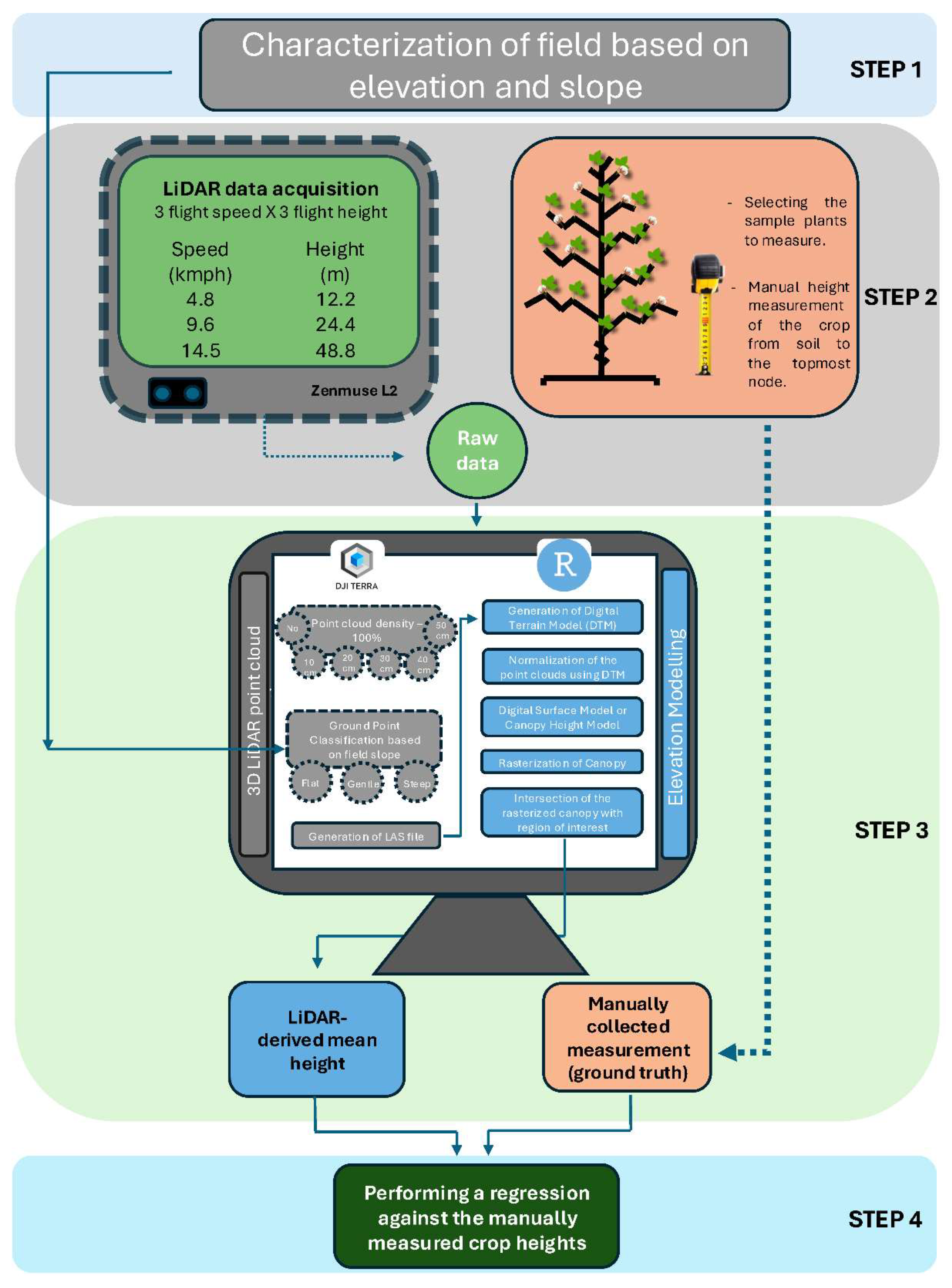
Figure 2.
Scatterplots of manual measured plant height (cm) and LiDAR-derived plant height (cm) for two locations, Watkinsville (green) and Midville (blue). Each panel represents data from one UAV flight altitude and speed combination. The solid black line represents the 1:1 line. The red line represents the regression line, with its equation shown inside each panel. The bold letters of the intercept and slope in the equation represent the significant difference from 0 and 1 respectively at p < 0.05. R2 is the coefficient of determination. MAE is the mean absolute error. RMSE is the root mean squared error.
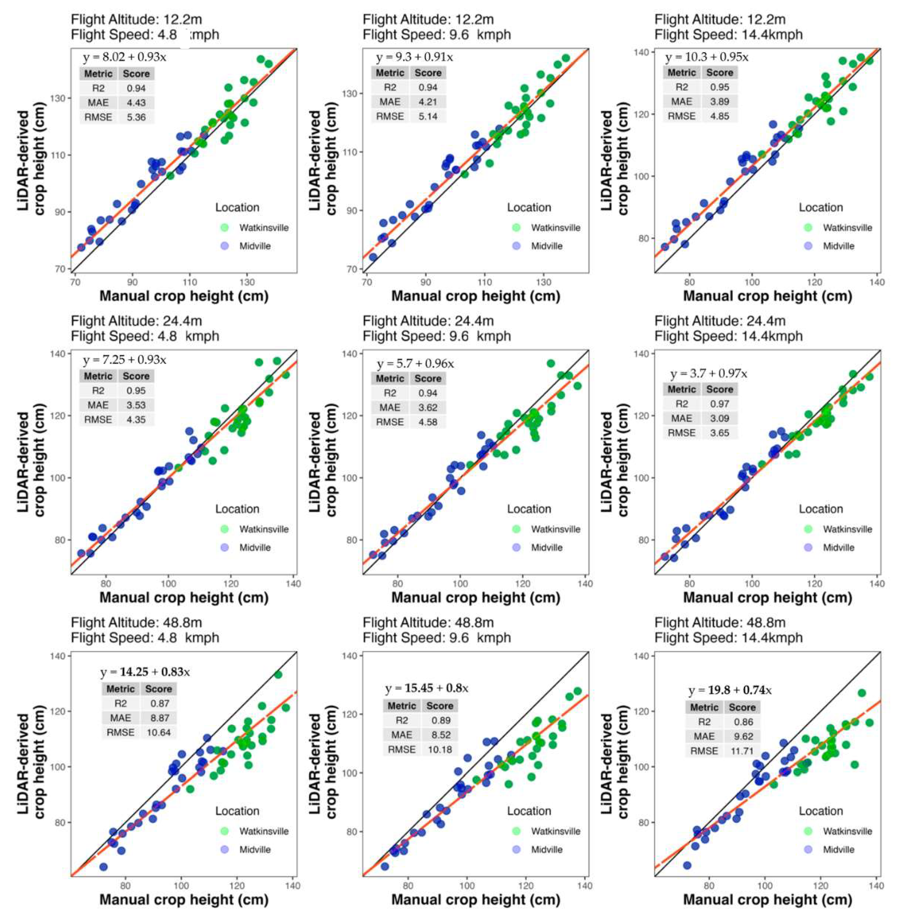
Figure 3.
Scatterplots of manual height and LiDAR-derived height in Watkinsville, GA. Each panel represents data from different sub-sampling grid sizes in Watkinsville. The title on left top of each graph shows the grid size used for sub-sampling. The solid black line represents the 1:1 line. The red line represents the regression line, with its equation showed inside each panel. The bold letters of the intercept and slope in the equation represent the significant difference from 0 and 1 respectively at p < 0.05. R2 is the coefficient of determination. MAE is the mean absolute error. RMSE is the root mean squared error.
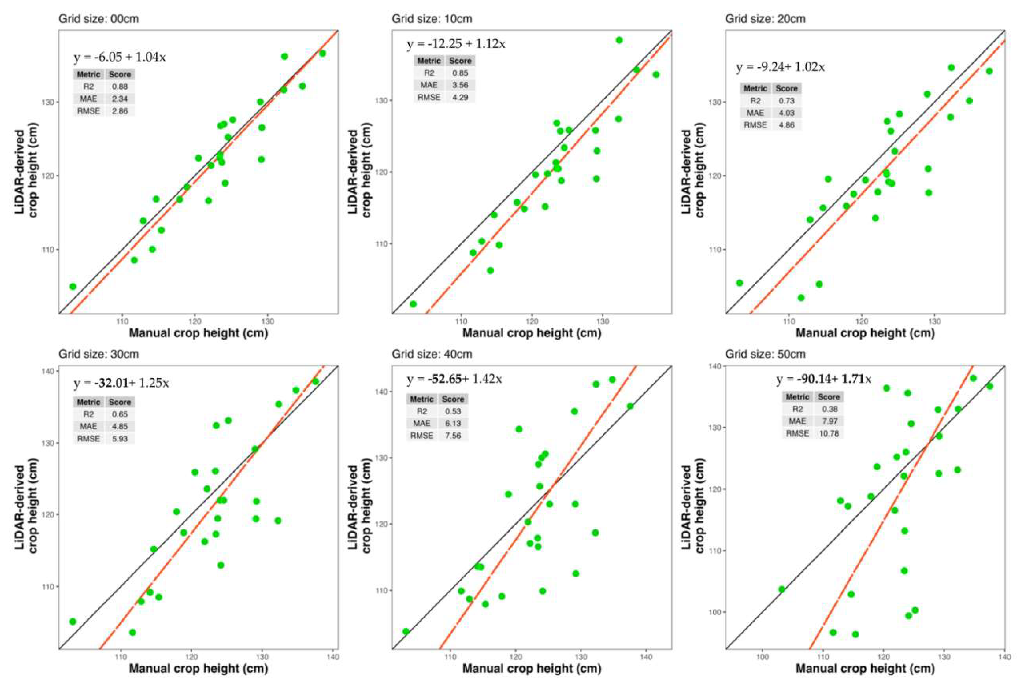
Figure 4.
Scatterplots of manual height and LiDAR-derived height in Midville, GA. Each panel represents data from different sub-sampling grid sizes in Midville. The title on left top of each graph shows the grid size used for sub-sampling. The solid black line represents the 1:1 line. The red line represents the regression line, with its equation showed inside each panel. The bold letters of the intercept and slope in the equation represent the significant difference from 0 and 1 respectively at p < 0.05. R2 is the coefficient of determination. MAE is the mean absolute error. RMSE is the root mean squared error.
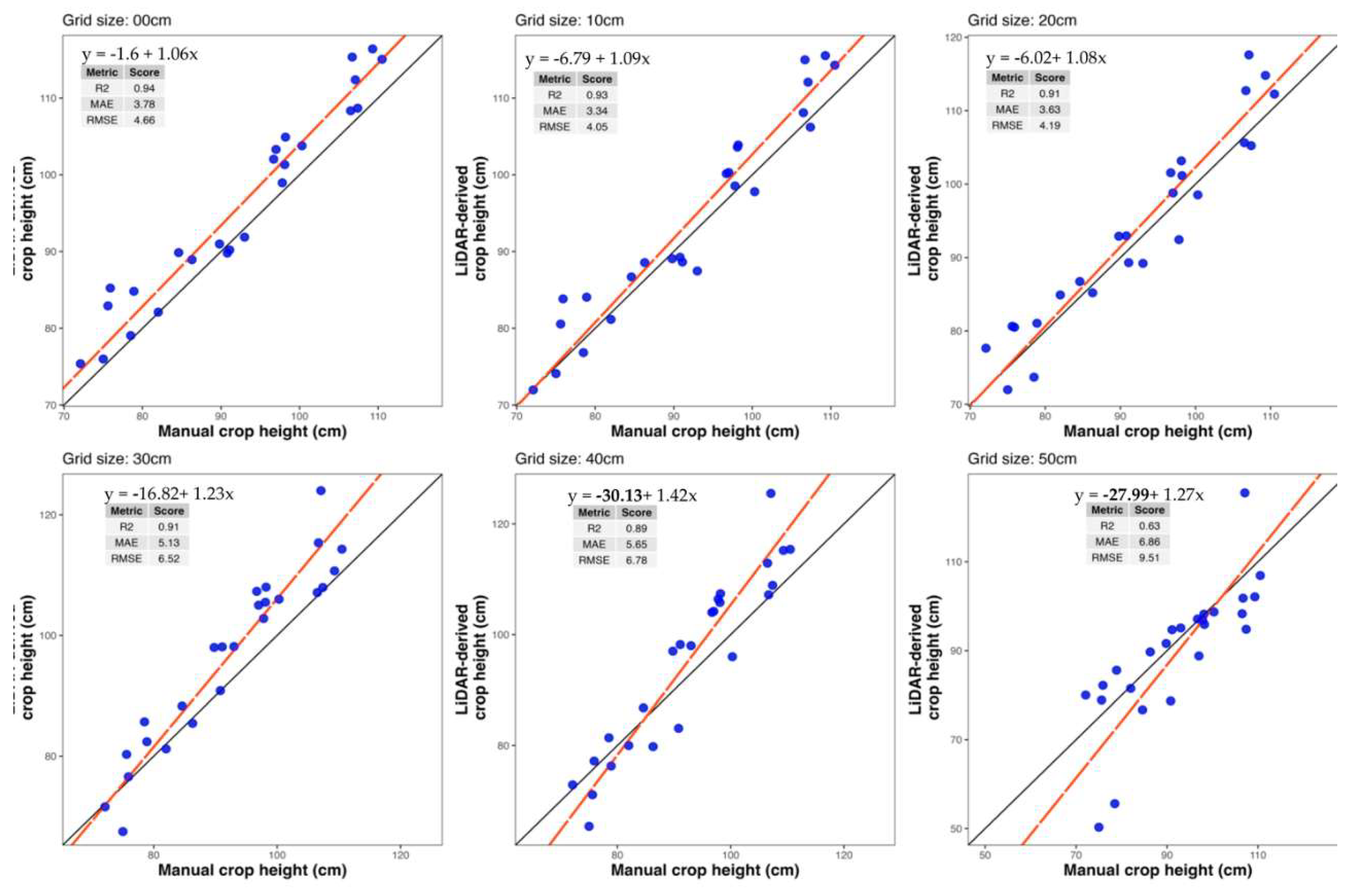
Figure 5.
Boxplots of differences between manual height and LiDAR-derived heights at three slope choices for point ground classification in DJI Terra software for two locations, Watkinsville (green) and Midville (blue). The y-axis represents the difference (manual - LiDAR), with values closer to zero indicating better agreement. Mean differences were determined at a significance level of 5% using the Least Significant Difference test. Treatments that share the same letter are not significantly different.
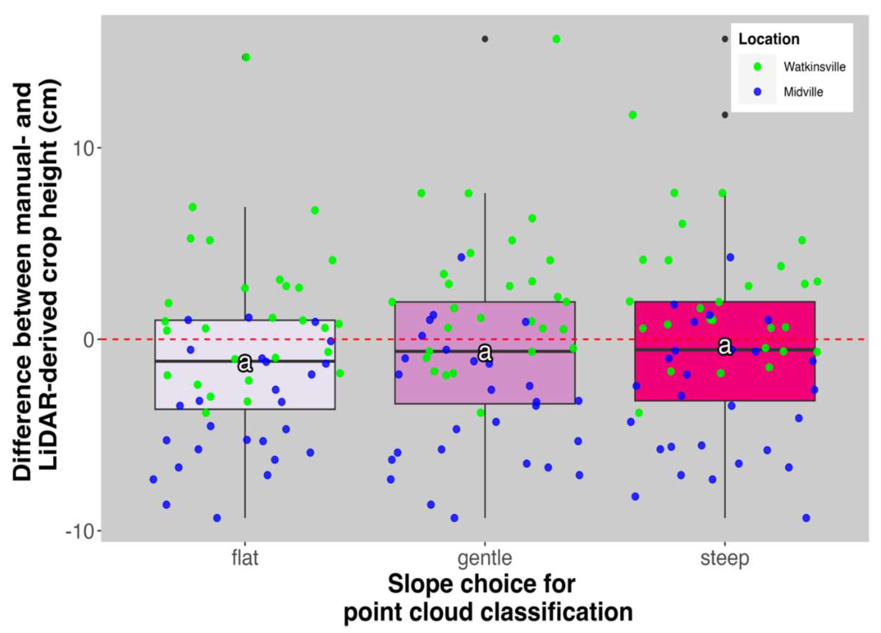
Figure 6.
Scatterplots of manual height and LiDAR-derived height. Each panel represents data from different slope-choices for point cloud classification for two locations, Watkinsville (green) and Midville (blue). The title on left top of each graph shows the slope-choice made. Solid black line represents the 1:1 line. Red line represents the regression line, with its equation showed inside each panel. The bold letters of the intercept and slope in the equation represent the significant difference from 0 and 1 respectively at p < 0.05. R2 is the coefficient of determination. MAE is the mean absolute error. RMSE is the root mean squared error.
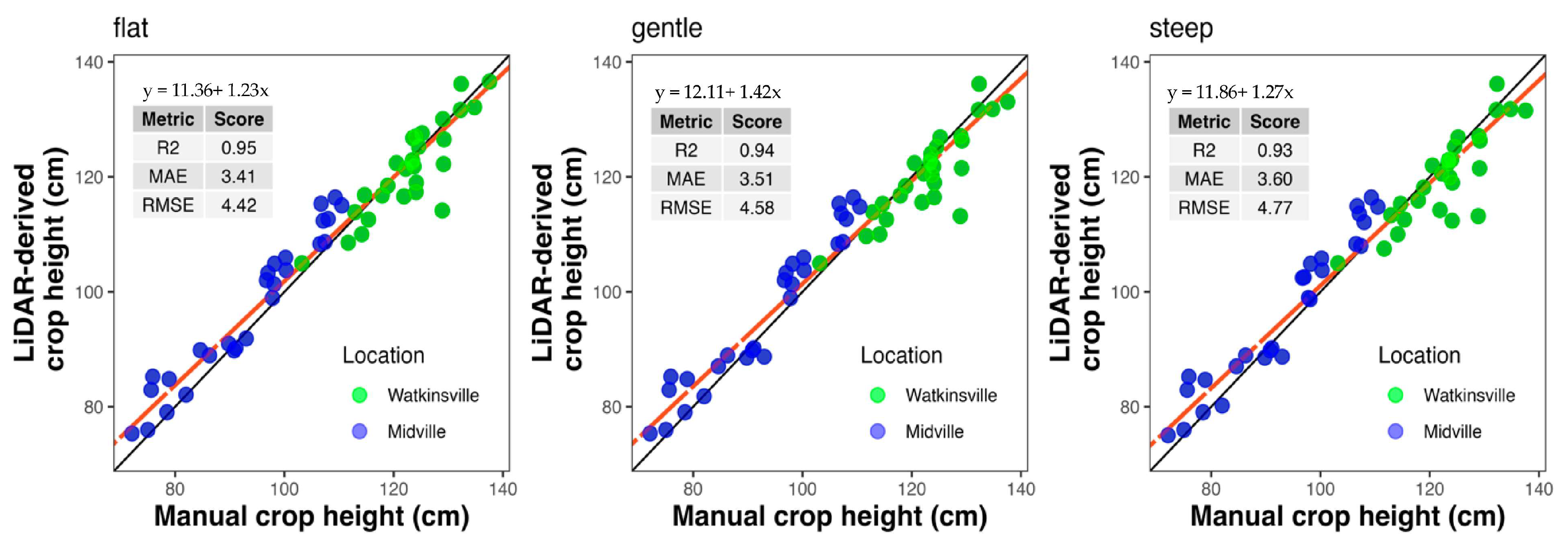

Table 1.
Effect of grid sub-sampling size on LiDAR point cloud density, processing time and file size with data obtained from Watkinsville.
Table 1.
Effect of grid sub-sampling size on LiDAR point cloud density, processing time and file size with data obtained from Watkinsville.
| Grid Sub-sampling (cm) |
Point Cloud Density (points/m2) |
Benchmarking time DJI Terra (3D LiDAR point cloud modelling) (sec) |
Benchmarking time R (Elevation Modelling) (sec) |
Total time for processing (sec) |
File size (mb) |
|---|---|---|---|---|---|
| 0 | 5834 | 143 | 63 | 206 | 812 |
| 10 | 539 | 101 | 55 | 156 | 149 |
| 20 | 110 | 83 | 37 | 120 | 35 |
| 30 | 41 | 82 | 21 | 103 | 13 |
| 40 | 20 | 80 | 19 | 99 | 6 |
| 50 | 21 | 77 | 14 | 91 | 4 |
Table 2.
Effect of grid sub-sampling size on LiDAR point cloud density, processing time and file size with data obtained from Midville.
Table 2.
Effect of grid sub-sampling size on LiDAR point cloud density, processing time and file size with data obtained from Midville.
| Grid Sub-sampling (cm) |
Point Cloud Density (points/m2) |
Benchmarking time DJI Terra (3D LiDAR point cloud modelling) (sec) |
Benchmarking time R (Elevation Modelling) (sec) |
Total time for processing (sec) |
File size (mb) |
|---|---|---|---|---|---|
| 0 | 2637 | 127 | 56 | 183 | 718 |
| 10 | 362 | 77 | 40 | 117 | 99 |
| 20 | 87 | 70 | 26 | 96 | 24 |
| 30 | 34 | 70 | 17 | 87 | 9 |
| 40 | 17 | 67 | 13 | 80 | 5 |
| 50 | 9 | 67 | 11 | 78 | 3 |
Disclaimer/Publisher’s Note: The statements, opinions and data contained in all publications are solely those of the individual author(s) and contributor(s) and not of MDPI and/or the editor(s). MDPI and/or the editor(s) disclaim responsibility for any injury to people or property resulting from any ideas, methods, instructions or products referred to in the content. |
© 2025 by the authors. Licensee MDPI, Basel, Switzerland. This article is an open access article distributed under the terms and conditions of the Creative Commons Attribution (CC BY) license (http://creativecommons.org/licenses/by/4.0/).
Copyright: This open access article is published under a Creative Commons CC BY 4.0 license, which permit the free download, distribution, and reuse, provided that the author and preprint are cited in any reuse.


