1. Introduction
The worldwide demand for electrical energy continues to increase and the govern- ments of different nations have to face several challenges to effectively respond to this demand. The first challenge is to provide energy for the growing proportion of the world’s population [
1,
2,
3]. While the second challenge lies in the production of this energy with- out causing environmental pollution, as well as causing climatic problems such as global warming [
4,
5,
6].
One of the ways to reduce green house gas emissions is to use renewable energy, such as wind and solar energies. The wind and the sun provide infinite amounts of energy without generating green house gases, unlike burning the fossil fuels electric power stations. Solar energy allows producing electricity from photovoltaic panels or solar thermal power stations, thanks to sunlight captured by solar panels. Solar energy is clean, does not emit any greenhouse gases and its source the sun, is free, inexhaustible and available everywhere in the world. Several countries around the globe are already at the forefront of renewable 33 energy technologies and generate a large part of their electricity from photovoltaic systems (PVS).
Like all other industrial process, a PVS can be subjected, during its operation, to various faults and anomalies leading to a drop in the performance of the system and even to the total unavailability of the system. These faults will deviously reduce the productivity of the installation [
7] and generate an additional cost of maintenance to restore the system to normal conditions. Hence, the importance of having a detecting and diagnosing faults in system photovoltaic installation, which contributes to raising production efficiency and reducing maintenance time and cost [
8].
There are many research contributions over the past decades in developing methods and algorithms for detecting and diagnosing faults in PV systems [
9,
10,
11]. According to references [
12,
13], these algorithms can be classified into three distinct categories, whereas in reference [
14], they are grouped into six categories.In this quick narration, the first categorization is adopted.
The first category encompasses all algorithms that use mathematical analysis and signal processing. Methods within this category heavily rely on the information extracted solely from the I-V characteristic, whether it pertains to a photovoltaic module (PVM), a PV string, or a photovoltaic array (PVA). Time Domain Reflectometry (TDR) is a technique utilized for identifying faulty photovoltaic modules within a photovoltaic array [
15].It has been employed to detect open circuits in grid-connected photovoltaic systems (GCPV) [
16]. Earth Capacitance Measurement (ECM) has been added to the TDR to identify the PV module disconnected from the PV string [
17]. Reference [
18] has demonstrated the applicability of the ECM algorithm in PV strings made of both silicon and amorphous silicon.
The second category comprises several algorithms characterized by two main phases: the detection phase utilizing a PV model and the subsequent diagnosis phase employing various methods, such as artificial intelligence [
19,
20,
21,
22]. These algorithms detect faults by comparing the measured values extracted from the considered PV generator with the simulated values from the PV model. The residual signal derived from this comparison can be utilized to detect degradation faults [
23] as well as various cases of line-line faults [
24].
The third category encompasses artificial intelligence and machine learning algorithms, including support vector machine (SVM) [
25,
26,
27,
28,
29], decision tree (DT) [
7,
30], random forest (RF) [
31,
32,
33], K-nearest neighbors (KNN) [
34,
35,
36], and artificial neural network (ANN) [
37,
38,
39]. Reference [
25] provides a comparison of efficiency and execution time among various multi-class strategies—such as one vs. all (OVA), adaptive directed acyclic graph (ADAG), and decision directed acyclic graph (DDAG)—utilizing SVM. The goal of SVM classification is to categorize data into four classes: module short circuit, inverse bypass diode module, shunted bypass module, and shadowing effect in a module.The OVA strat- egy has demonstrated significant superiority over others in terms of efficiency, achieving an 88.33% accuracy rate. In reference [
26], the SVM algorithm was employed to detect series faults of 10%, 50%, 70%, and 90% under sunny, cloudy, and rainy weather conditions. The recorded accuracies were 88.3%, 91.5%, and 75.3%, respectively.In reference [
27], both the CPA and SVM algorithms were utilized to identify four operating states: normal, open circuit, short circuit, and partial shading. The authors concluded that with k = 6 (number of dimension), the algorithm achieved an accuracy rate of 100%. In reference [
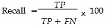
28], the authors used the SVM algorithm to detect faults such as open circuit, short circuit, and lack of solar radiation. The algorithm requires four inputs:short circuit current Isc, open circuit voltage Voc, and coordinates of maximum power point Impp and Vmpp. The algorithm’s efficiency and accuracy were enhanced by employing k-fold cross-validation. The drawback with the mentioned algorithms is that their authors solely relied on accuracy as the criterion 83 for evaluation, whereas employing different metrics like precision and recall could offer a 84 more comprehensive assessment of the algorithms.
In [
7], a novel approach based on DT algorithm is presented. This approach comprises two models: the first model detects faults, while the second model diagnoses four different fault types: short circuit, string, line-line, and free faults. The accuracy rates for the first and second models are 99.86% and 99.80%, respectively. Notably, although a confusion matrix was calculated, precision and recall metrics were not evaluated.The utilization of the random forest algorithm for fault detection and classification in PV systems is highlighted in [
31]. The method introduced in this study necessitates the current from each string in the PV array, along with the PV array voltage, as features. Successfully, the algorithm detects and diagnoses four different faults: degradation, partial shading, line-to-line, and short circuit faults. Authors have employed the grid-search method to optimize the random forest parameters. In order to evaluate this method, experimental and simulation samples were used.
The accuracy of this method reached 99%. Another method was developed based on RF to detect and diagnose faults in photovoltaic systems [
32]. A set of criteria were used to evaluate the method, which are computation time, accuracy, and F1 score. In [
34], a modified KNN algorithm was proposed and applied to photovoltaic systems for fault detection and diagnosis. The main modification made by the researchers in this work is to facilitate the selection of the appropriate K value in addition to the distance function. This modification greatly contributed to the increase in the classification speed. Moreover, in [
35], an interesting technique, that uses the KNN algorithm, has been developed to detect multiple faults, including line to line and partial shading faults. Remarkably, this method only relies on data from the datasheet and achieves an accuracy rate of 99%. Another model developed is based on the combination of KNN and Exponential Weighted Moving Average (EWMA) [
36]. The KNN aims to detect faults on the DC side of the PV system, while the EMWA works to diagnose those faults. Researchers in [
38] built a two-stage classifier: the first stage is a model of the PV system to detect faults, while the second stage devoted for diagnosis purposes where is two artificial neural networks were used to identify eight different faults.In [
39], another approach based on artificial neural networks for fault detection and diagnosis in PV systems is introduced. The authors utilized an ANN with radial basis function (RBF) architecture, relying on two features: power generated and solar irradiance. The achieved accuracy in this study was 97.9% for the 2.2 KW PV system and 97% for the 4.16 KW PV system.
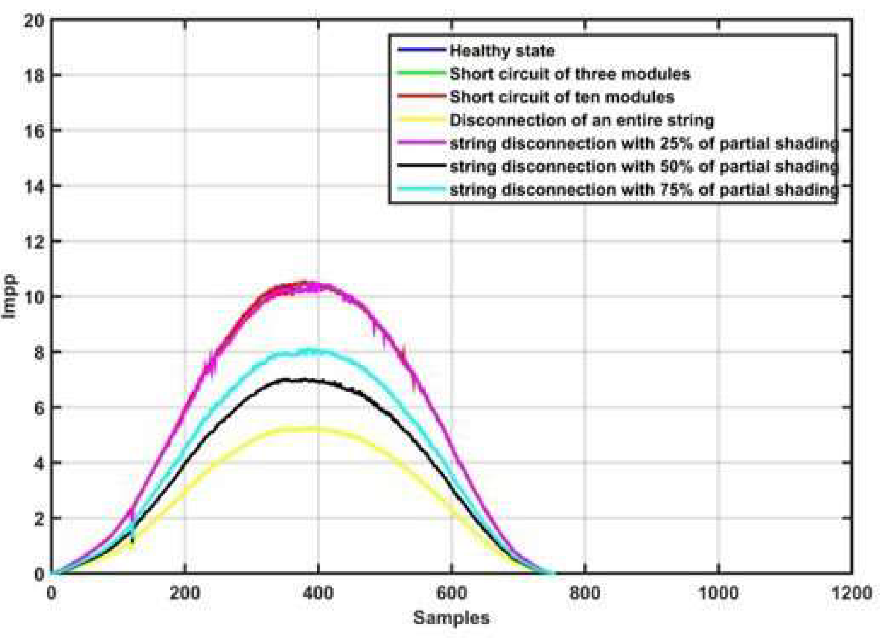
In this work, a novel fault detection and diagnosis algorithm is developed and de signed in the DC of PV systems. This methodology is based on an innovative tree algorithm that mainly depends on calculating Euclidean distances to detect faults when they occur, effectively. At first, the algorithm classifies the data into two classes so that all the distances between a random point in space and the entire data set are calculated. Then, in each class, the minimum and maximum distances are extracted. After that, all the distances are arranged in ascending order to show one case out of 5 possible cases. Based on the apparent case, the data are classified. The algorithm needs 4 features to function properly: solar radi ation, temperature, and current and voltage at the maximum power point. This algorithm has been implemented to seven different classes: normal operation, series disconnection, short circuit for 3 and 10 modules and three other classes for series disconnection with partial shading of 25%, 50% and 75%. The efficiency and effectiveness of the methodology is clearly demonstrated by the accuracy rate achieved which exceeds 97%. In order to further evaluate the algorithm, a comparative study was conducted between the proposed algorithm and several well-known algorithms (support vector machine, K nearest neighbor, decision tree and random forest). The comparison results show a clear superiority of the developed algorithm in terms of accuracy, precision and recall.
This paper is organized as follows:
Section 2 is dedicated to introducing the developed algorithm, while
Section 3 explains the database used and its different categories.
Section 4 reveals the classification strategy followed in this work. In Section Five, the results obtained are presented and discussed. The last section of this paper presents a summary of the work done in this research paper
2. Proposed Euclidean-Based Decision Tree Classification Algorithm
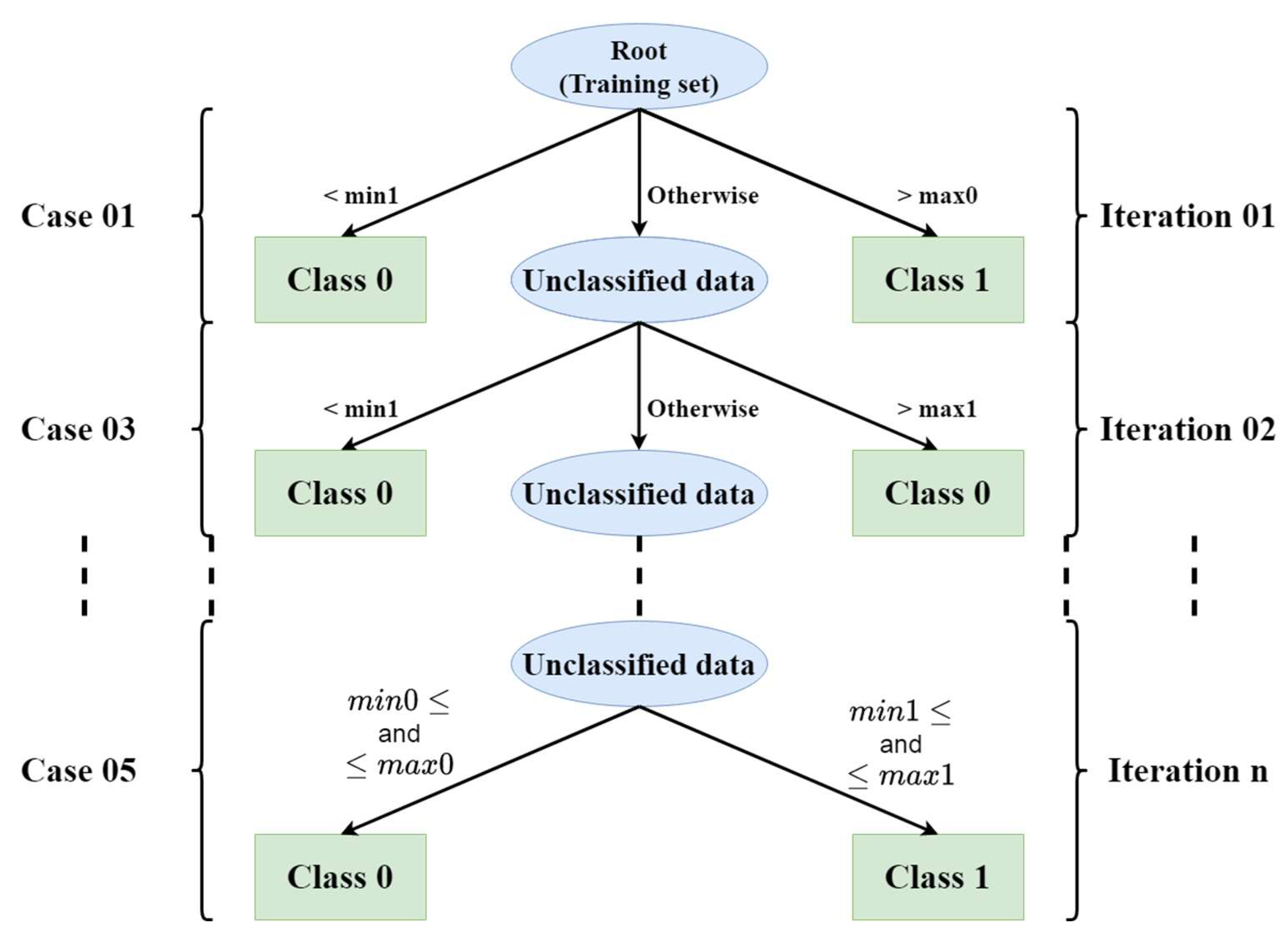
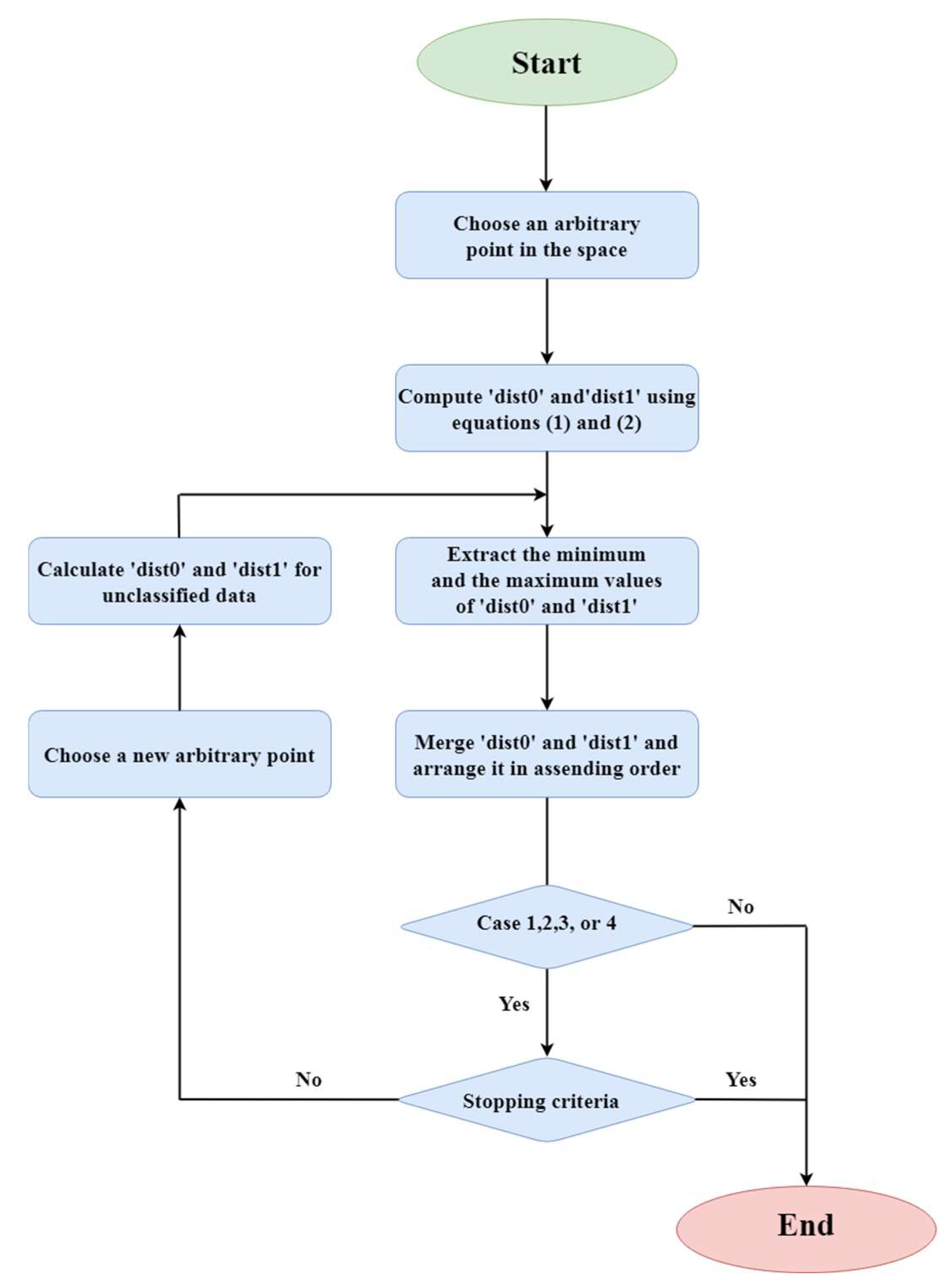
Despite the similarities between the proposed algorithm and the decision trees in their data splitting approach, the key distinction lies in using the Euclidean distance for partitioning data instead of the Gini index. Initially, a training dataset, comprising values for N features for each of the two classes (class 0 and class 1), is created.Then, the following steps are performed:
Choose an arbitrary point (x1, x2, ..., xN ) in an N-dimensional space.
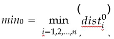
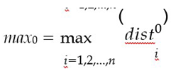
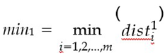
Using equations 4.1 and 4.2, compute the Euclidean distances between the chosen point and all samples within the training dataset for each respective class:
(x0 , x0 , ..., x0 ) and (x1 , x1 , ..., x1 ) represent the ith samples of class 0 and class 1, i1 i2 in i1 i2 im respectively. n denotes the number of samples in class 0, while m denotes the number of samples in class 1.
- 3.
Determine the minimum and maximum distances for each class:
- 4.
-
Among the following five cases, one may arise:
-
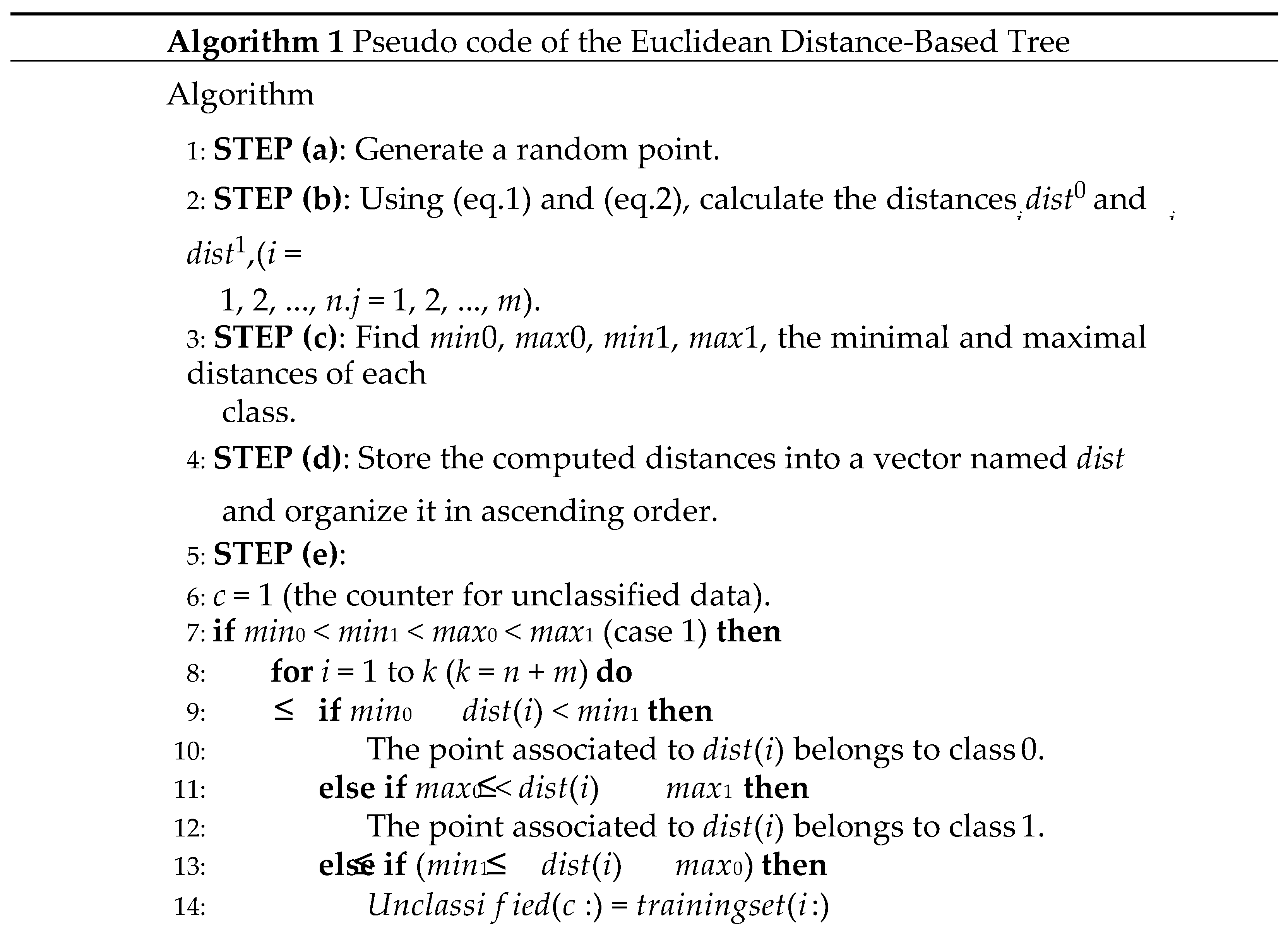
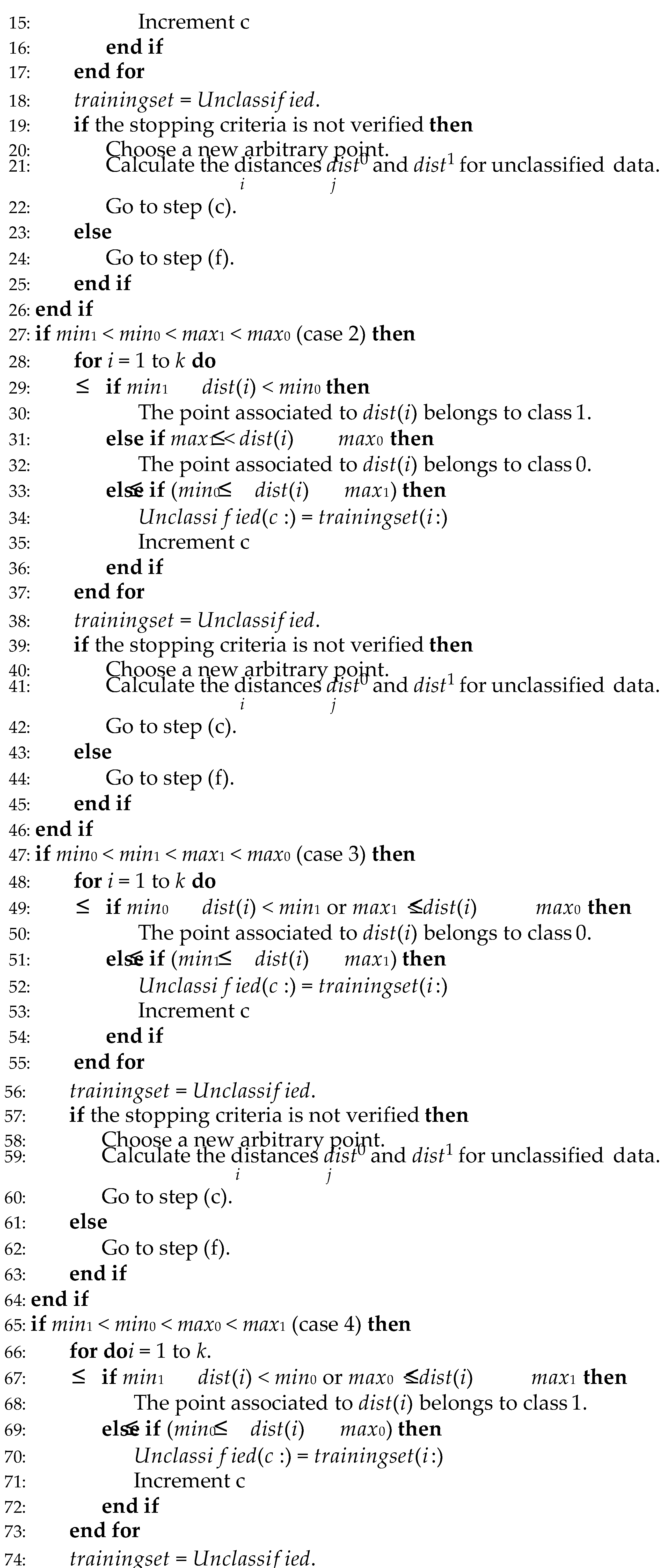
case 1: min0 < min1 < max0 < max1
- -
Training samples having distances within the interval [min0, min1[ belong to class 0 (pure data in class 0).
- -
Training samples having distances within the interval ]max0, max1] belong to class 1 (pure data in class 1).
- -
Training samples having distances within the interval [min1, max0] can not be classified, therefore another random point must be chosen for their classification.
-
case 2: min1 < min0 < max1 < max0
- -
Training samples having distances within the interval [min1, min0[ belong to class 1 (pure data in class 1).
- -
Training samples having distances within the interval ]max1, max0] belong to class 0 (pure data in class 0).
- -
Training samples having distances within the interval [min0, max1] can not be classified, therefore another random point must be chosen for their classification.
-
case 3: min0 < min1 < max1 < max0
- -
Training samples having distances within the interval [min0, min1[ or ]max1, max0] belong to class 0.
- -
Training samples having distances within the interval [min1, max1] can not be classified, therefore another random point must be chosen for their classification.
-
case 4: min1 < min0 < max0 < max1
- -
Training samples having distances within the interval [min1, min0[ or ]max0, max1] belong to class 1.
- -
Training samples having distances within the interval [min0, max0] can not be classified, therefore another random point must be chosen for their classification.
-
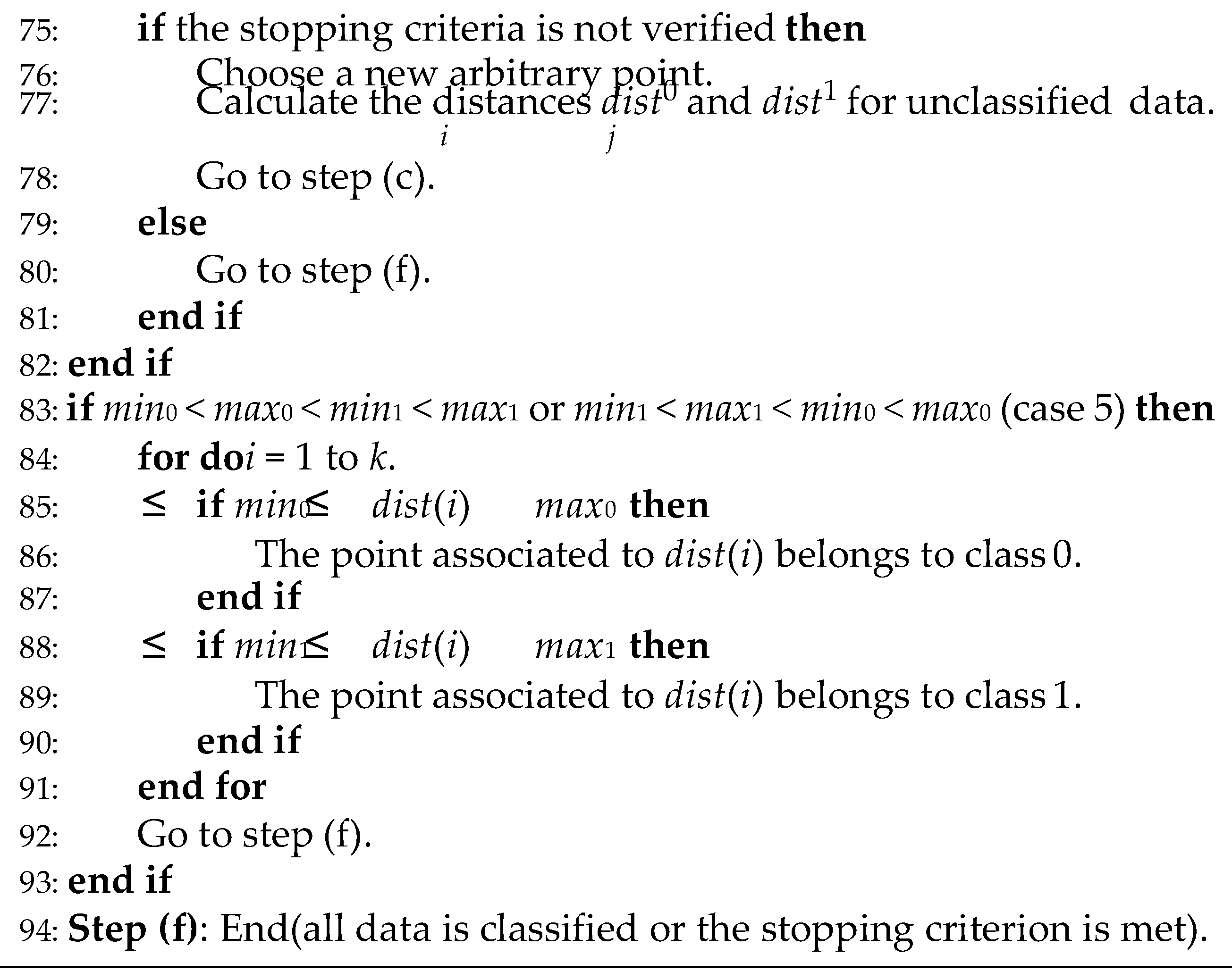
case 5: min0 < max0 < min1 < max1 or min1 < max1 < min0 < max0
- -
Training samples having distances within the interval [min0, max0] belong to class 0.
- -
Training samples having distances within the interval [min1, max1] belong to class 1.
- 5.
-
If the case that occurred in the previous step is case 1, 2, 3, or 4:
Choose another random point (x1, x2, . . . , xN ).
Using equations 4.1 and 4.2, compute the Euclidean distances between the chosen point and the unclassified samples within the training dataset for each respective class.
Go to step 3.
- 6.
The algorithm iterates through steps (c) to (e) until all data is classified (case 5) or the stopping criterion is met. It employs early stopping as its stopping criterion to effectively mitigate overfitting without compromising the accuracy of the algorithm [
40,
41,
42].
To address the overfitting issue, the difference between test accuracy and training accuracy is calculated. This difference should be minimal (less than 3% for example). If it exceeds this threshold, the training process is halted.
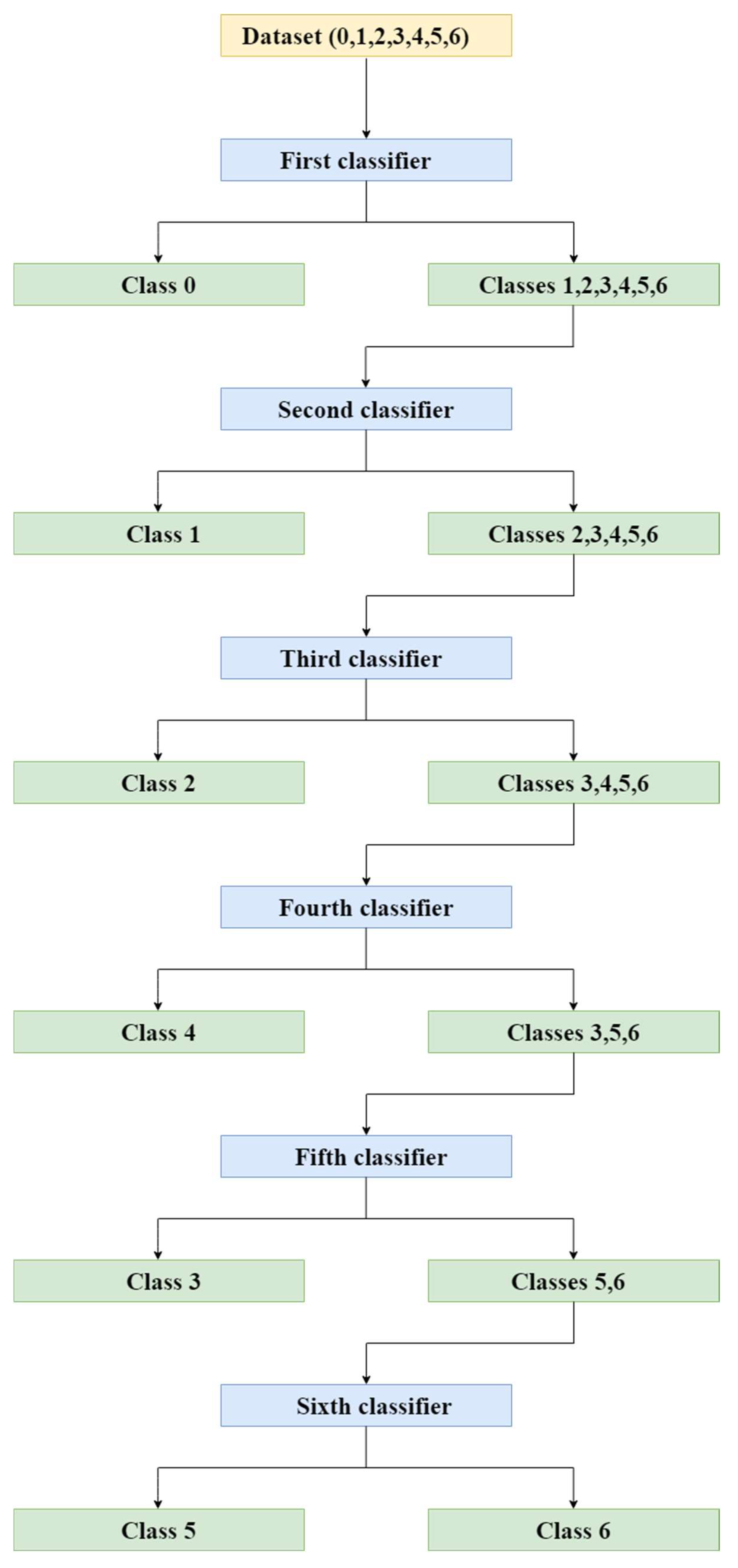
Figure 1 provides a graphical illustration of the proposed algorithm depicting a given possible situation.
The flowchart of the algorithm is given in
Figure 2.
The pseudo code of the proposed algorithm is given below:
Figure 1.
Flowchart of the proposed algorithm.
Figure 1.
Flowchart of the proposed algorithm.
Figure 2.
Flowchart of the proposed algorithm.
Figure 2.
Flowchart of the proposed algorithm.
Figure 3.
Impp for various operating states of the PVA.
Figure 3.
Impp for various operating states of the PVA.
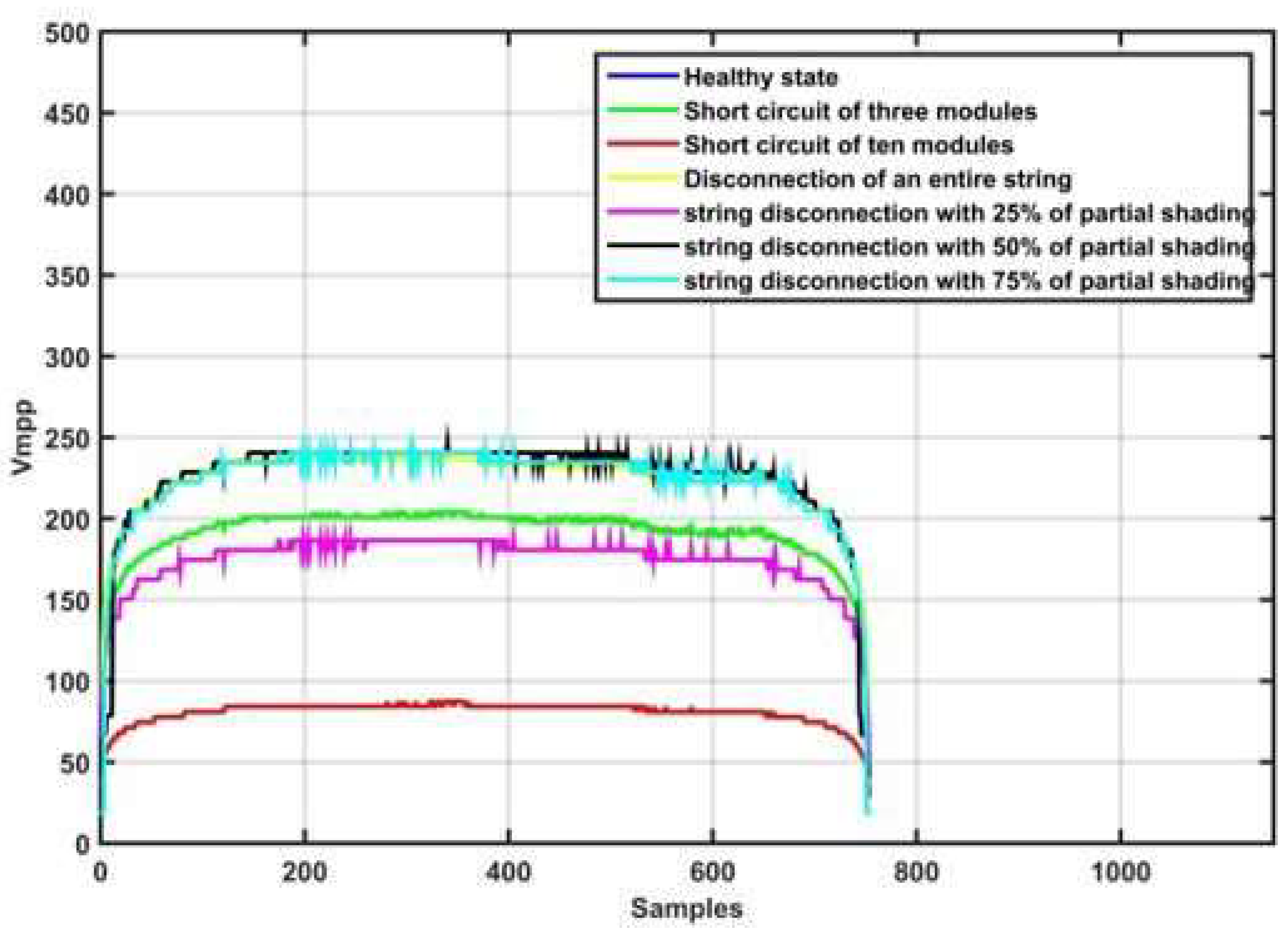
Figure 4.
Vmpp for various operating states of the PVA.
Figure 4.
Vmpp for various operating states of the PVA.
Figure 5.
Fault detection and diagnosis flowchart.
Figure 5.
Fault detection and diagnosis flowchart.
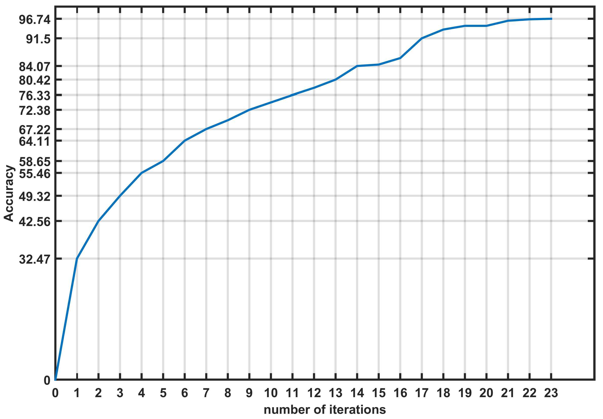
Figure 6.
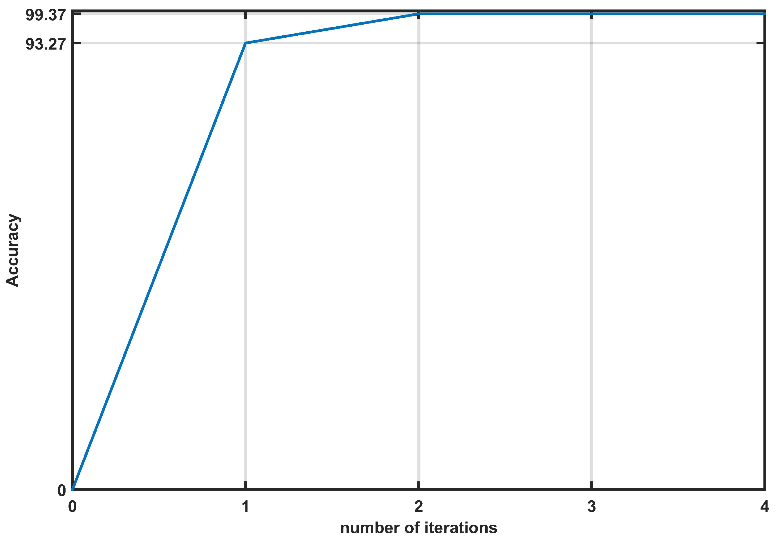
Evolution of accuracy for the first classifier.
Figure 6.
Evolution of accuracy for the first classifier.
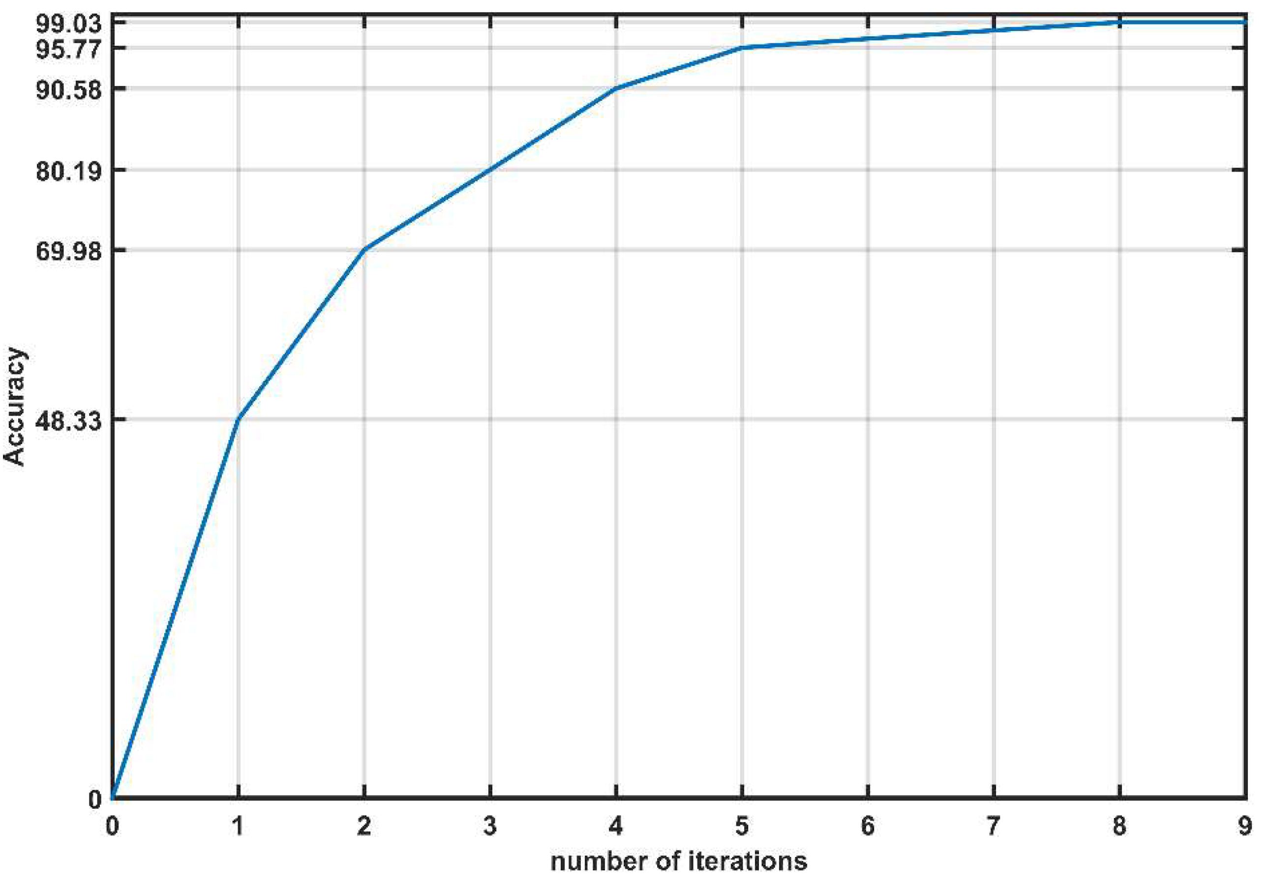
Figure 7.
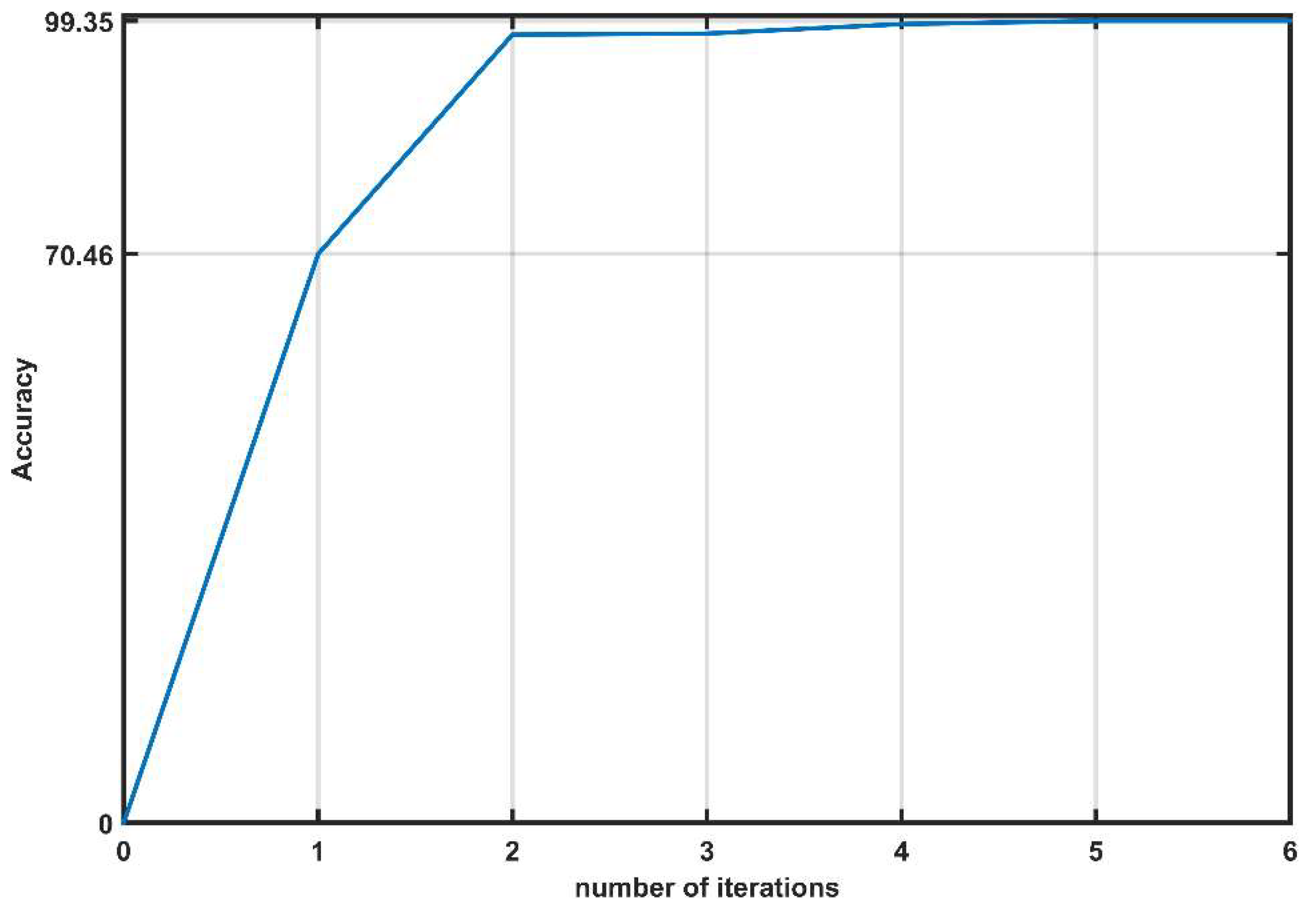
Evolution of accuracy for the second classifier.
Figure 7.
Evolution of accuracy for the second classifier.
Figure 8.
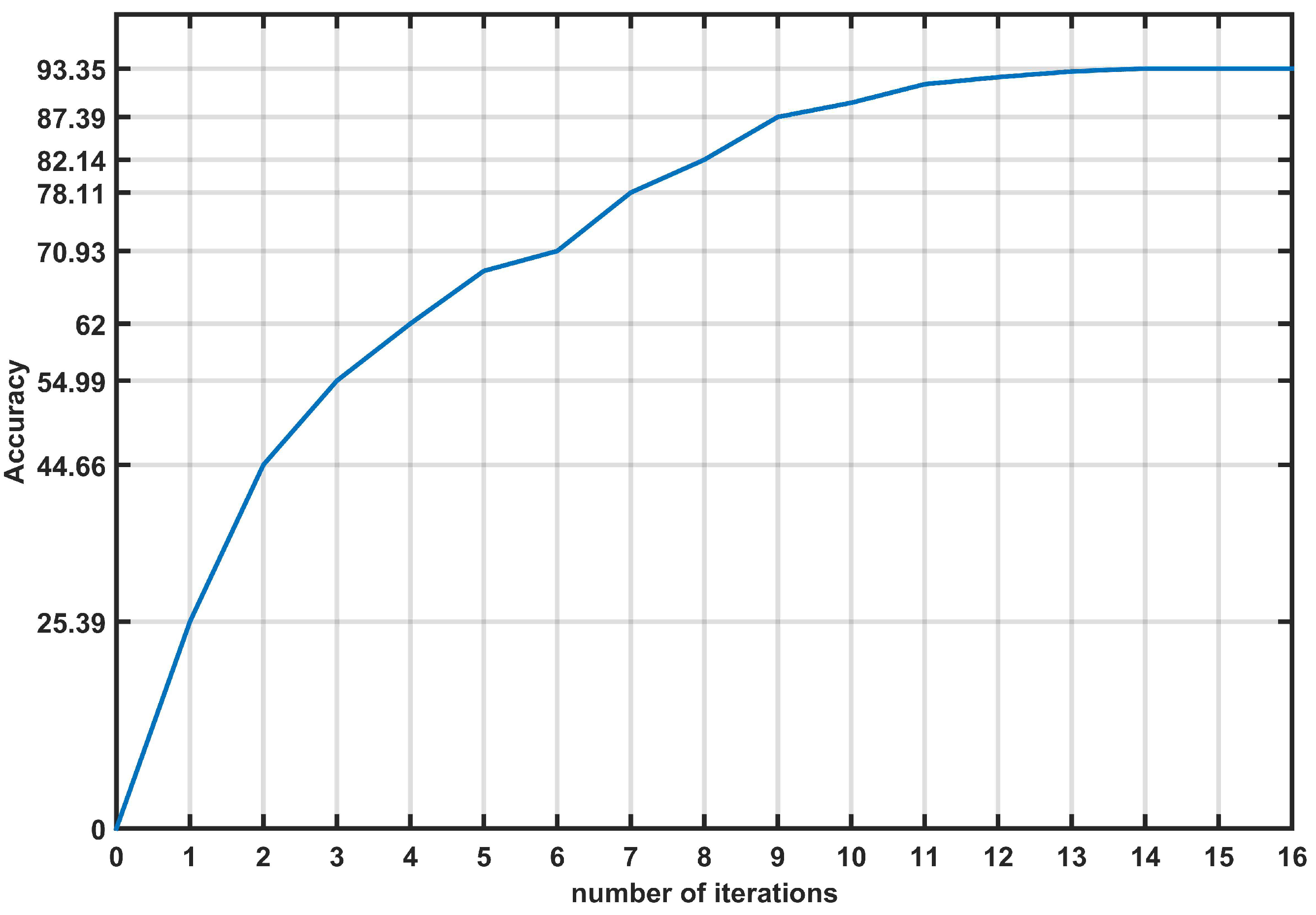
Evolution of accuracy for the third classifier.
Figure 8.
Evolution of accuracy for the third classifier.
Figure 9.
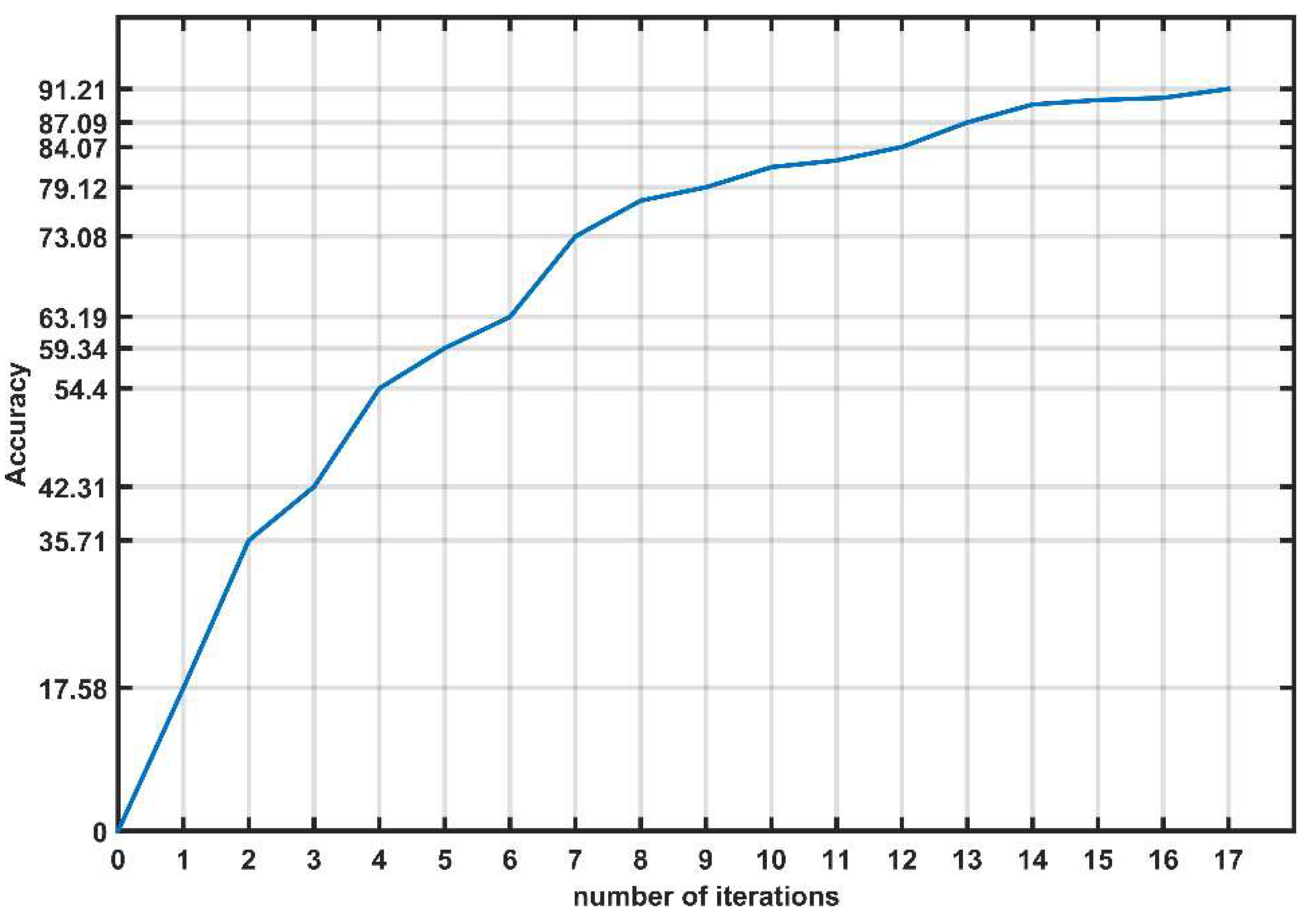
Evolution of accuracy for the forth classifier.
Figure 9.
Evolution of accuracy for the forth classifier.
Figure 10.
Evolution of accuracy for the fifth classifier.
Figure 10.
Evolution of accuracy for the fifth classifier.
Figure 11.
Evolution of accuracy for the sixth classifier.
Figure 11.
Evolution of accuracy for the sixth classifier.
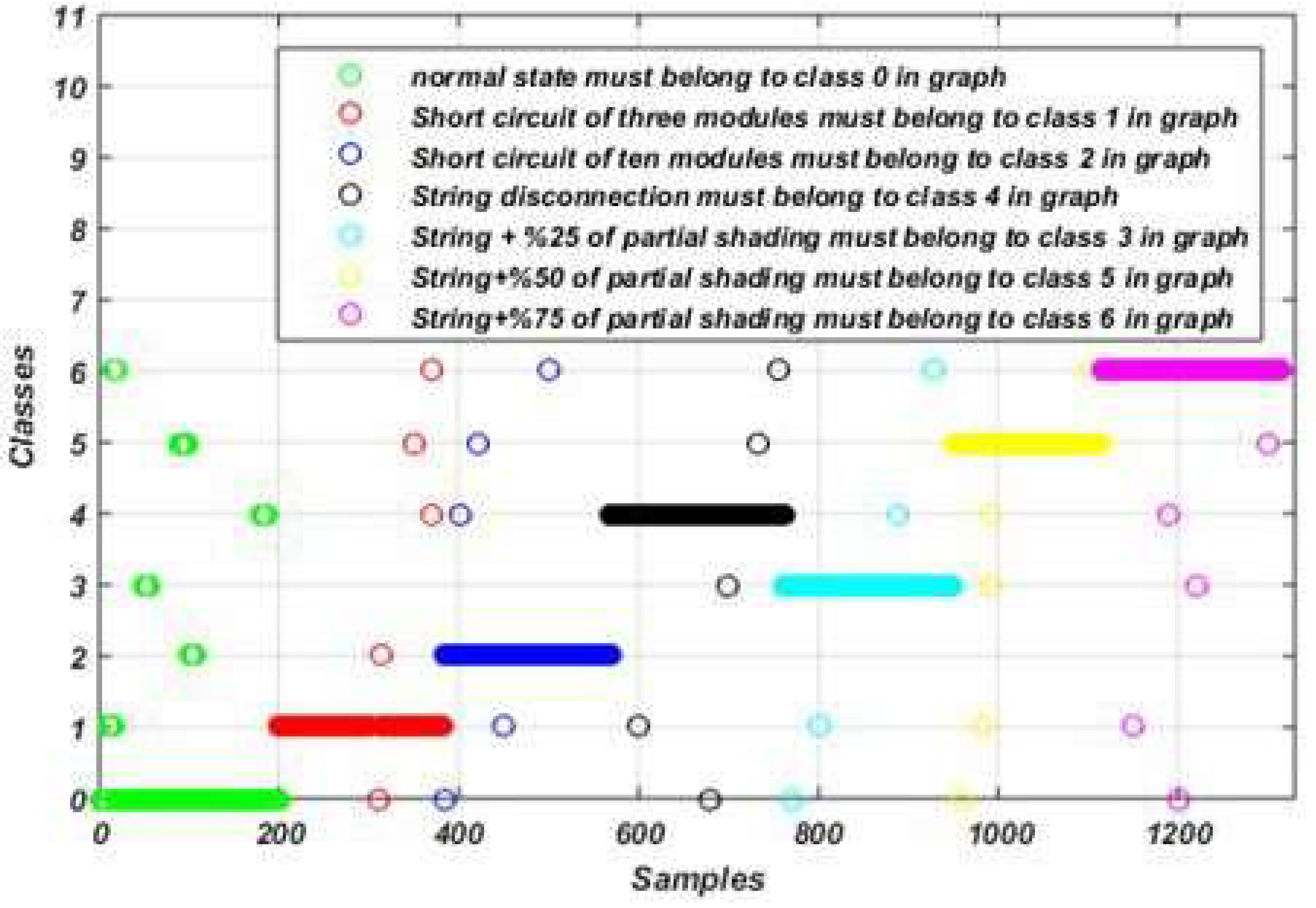
Figure 12.
Fault detection and diagnosis results using the proposed algorithm-based model.
Figure 12.
Fault detection and diagnosis results using the proposed algorithm-based model.
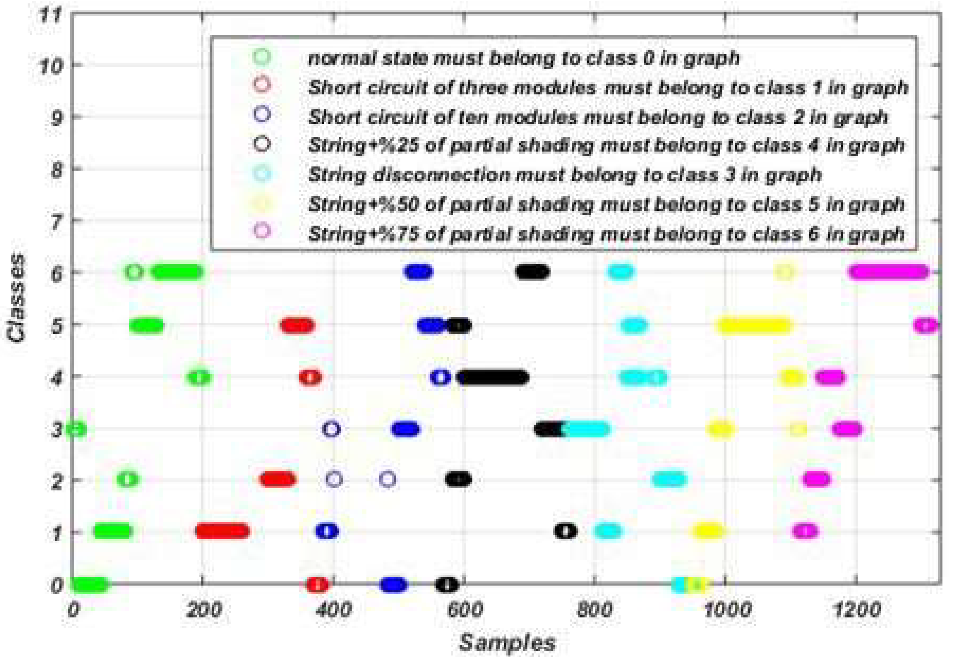
Figure 13.
Fault detection and diagnosis results using the SVM algorithm-based model.
Figure 13.
Fault detection and diagnosis results using the SVM algorithm-based model.
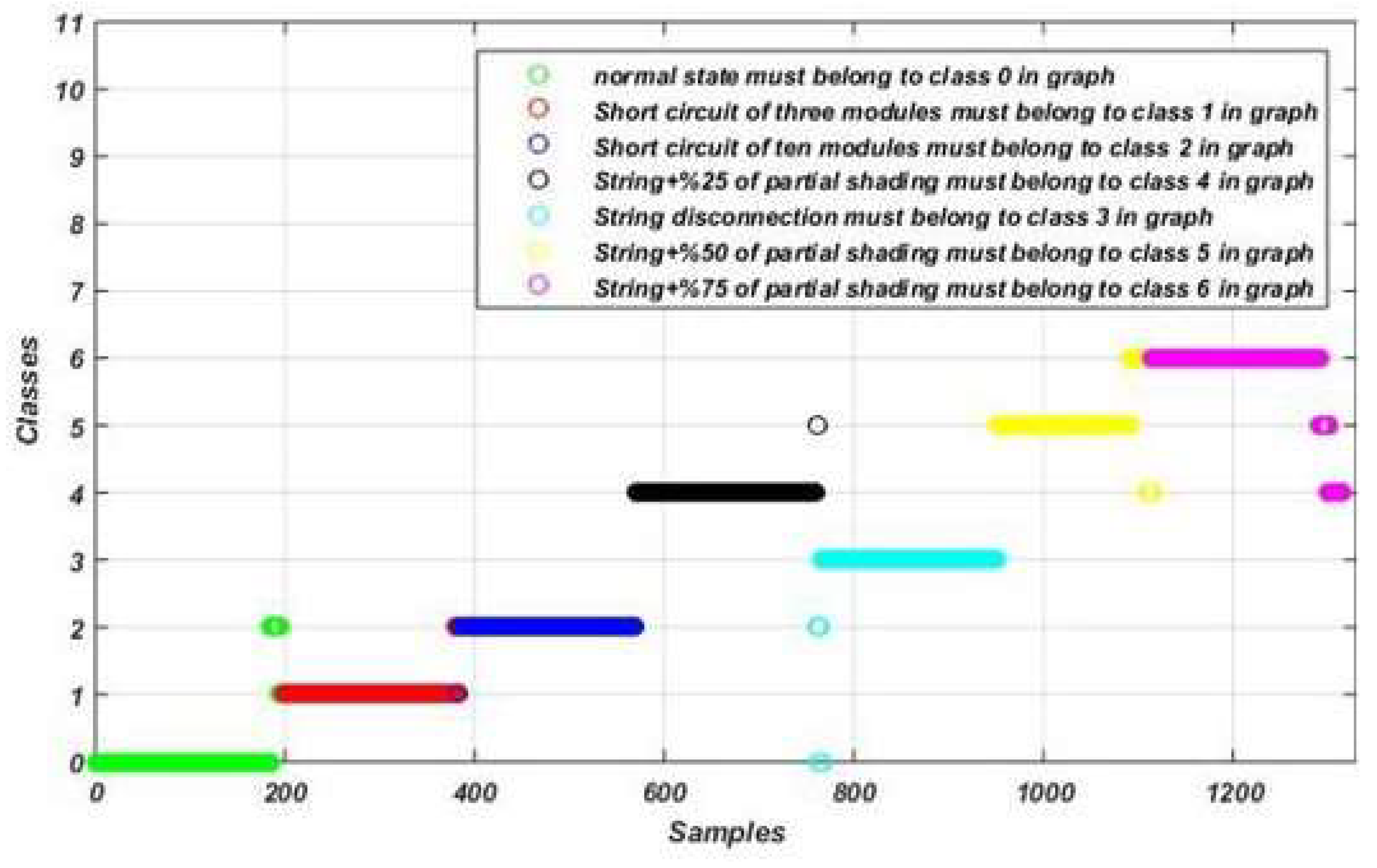
Figure 14.
Fault detection and diagnosis results using the DT algorithm-based model.
Figure 14.
Fault detection and diagnosis results using the DT algorithm-based model.
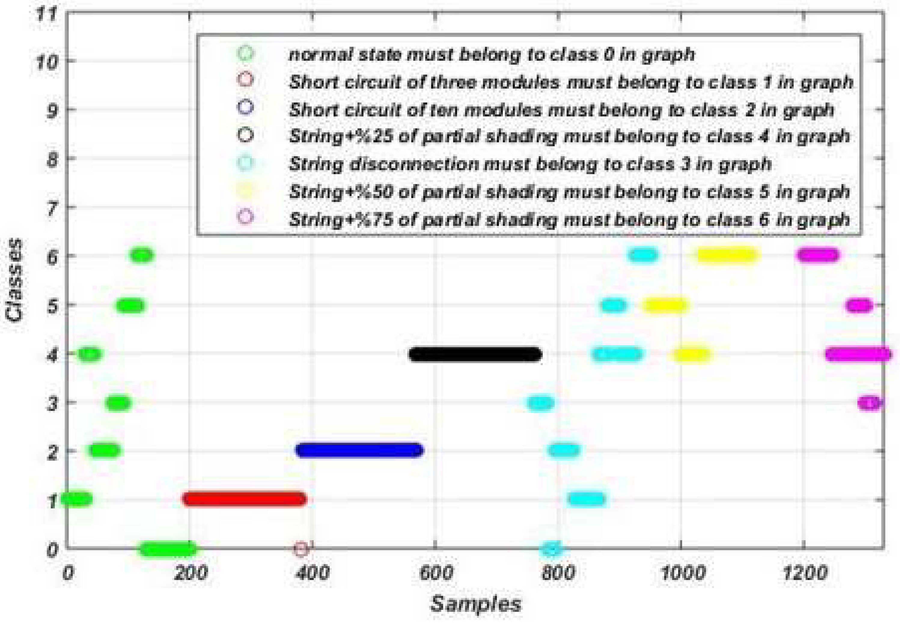
Figure 15.
Fault detection and diagnosis results using the RF algorithm-based model.
Figure 15.
Fault detection and diagnosis results using the RF algorithm-based model.
Figure 16.
Fault detection and diagnosis results using the KNN algorithm-based model.
Figure 16.
Fault detection and diagnosis results using the KNN algorithm-based model.
Table 1.
Operating states and their labels.
Table 1.
Operating states and their labels.
| Class name |
Label |
| Normal operation |
Class 0 |
| Short circuit of three modules |
Class 1 |
| Short circuit of ten modules |
Class 2 |
| String disconnection |
Class 3 |
| String disconnection with 25% of partial shading |
Class 4 |
| String disconnection with 50% of partial shading |
Class 5 |
| String disconnection with 75% of partial shading |
Class 6 |
Table 2.
Confusion matrix.
Table 2.
Confusion matrix.
| Real class labels |
Predicted label: A |
Predicted label: B |
| Class A |
TP |
FN |
| Class B |
FP |
TN |
Table 3.
Confusion matrices for the obtained model.
Table 3.
Confusion matrices for the obtained model.
| |
TP |
FN |
FP |
TN |
| Classifier 1 |
1107 |
19 |
29 |
168 |
| Classifier 2 |
947 |
3 |
4 |
178 |
| Classifier 3 |
762 |
1 |
3 |
183 |
| Classifier 4 |
570 |
3 |
1 |
190 |
| Classifier 5 |
354 |
13 |
10 |
179 |
| Classifier 6 |
177 |
20 |
5 |
155 |
Table 4.
Metrics values for the obtained model.
Table 4.
Metrics values for the obtained model.
| |
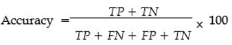
Accuracy (%) |
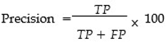
Precision (%) |
Recall (%) |
| Classifier 1 |
97 |
97 |
98 |
| Classifier 2 |
99 |
100 |
100 |
| Classifier 3 |
100 |
100 |
100 |
| Classifier 4 |
99 |
100 |
99 |
| Classifier 5 |
96 |
97 |
99 |
| Classifier 6 |
93 |
97 |
90 |
| Average values |
97.33
|
99 |
97 |
Table 5.
Confusion matrices for the obtained model using the four algorithms.
Table 5.
Confusion matrices for the obtained model using the four algorithms.
| |
SVM |
DT |
RF |
KNN |
| Classifier 1 |
TP |
1104 |
113 |
1119 |
1107 |
| |
FN |
15 |
6 |
8 |
12 |
| |
FP |
165 |
23 |
15 |
155 |
| |
TN |
34 |
176 |
176 |
44 |
| Classifier 2 |
TP |
1086 |
950 |
950 |
1078 |
| |
FN |
0 |
3 |
1 |
1 |
| |
FP |
122 |
3 |
1 |
1 |
| |
TN |
61 |
180 |
180 |
182 |
| Classifier 3 |
TP |
1021 |
765 |
764 |
892 |
| |
FN |
0 |
2 |
0 |
0 |
| |
FP |
103 |
0 |
1 |
0 |
| |
TN |
84 |
186 |
186 |
187 |
| Classifier 4 |
TP |
927 |
566 |
568 |
696 |
| |
FN |
0 |
3 |
1 |
0 |
| |
FP |
107 |
0 |
0 |
0 |
| |
TN |
90 |
196 |
196 |
196 |
| Classifier 5 |
TP |
796 |
364 |
371 |
508 |
| |
FN |
57 |
10 |
4 |
1 |
| |
FP |
131 |
7 |
3 |
167 |
| |
TN |
50 |
185 |
183 |
157 |
| Classifier 6 |
TP |
631 |
29 |
36 |
105 |
| |
FN |
112 |
172 |
175 |
73 |
| |
FP |
84 |
202 |
202 |
201 |
| |
TN |
90 |
|
102 |
|
Table 6.
Metrics values (in percentage) for the obtained model using the four algorithms.
Table 6.
Metrics values (in percentage) for the obtained model using the four algorithms.
| |
SVM |
DT |
RF |
KNN |
| Classifier 1 Accuracy |
86 |
98 |
99 |
87(K=7) |
| Precision |
87 |
98 |
99 |
88 |
| Recall |
99 |
99 |
100 |
99 |
| Classifier 2 Accuracy |
90 |
99 |
100 |
100(K=1) |
| Precision |
90 |
100 |
100 |
100 |
| Recall |
100 |
100 |
100 |
100 |
| Classifier 3 Accuracy |
91 |
100 |
100 |
100(K=3) |
| Precision |
91 |
100 |
100 |
100 |
| Recall |
100 |
100 |
100 |
100 |
| Classifier 4 Accuracy |
90 |
100 |
100 |
100(K=2) |
| Precision |
90 |
100 |
100 |
100 |
| Recall |
100 |
99 |
100 |
100 |
| Classifier 5 Accuracy |
82 |
97 |
99 |
76(K=35) |
| Precision |
86 |
98 |
99 |
75 |
| Recall |
93 |
97 |
99 |
100 |
| Classifier 6 Accuracy |
78 |
64 |
63 |
59(K=1) |
| Precision |
88 |
87 |
85 |
80 |
| Recall |
84 |
54 |
53 |
60 |
| Average values Accuracy |
85.33 |
97.16 |
93.50 |
87 |
| Precision |
88.65 |
91.50 |
97.16 |
90.50 |
| Recall |
96 |
93.50 |
92 |
93.16 |
Table 7.
Metrics average values.
Table 7.
Metrics average values.
| |
Accuracy (%) |
Precision (%) |
Recall (%) |
| The proposed |
|
|
|
| algorithm |
97.33
|
98.66
|
97.5
|
| SVM |
85.33 |
88.65 |
96 |
| DT |
93 |
97.16 |
91.50 |
| RF |
93.50 |
97.16 |
92 |
| KNN |
87 |
90.50 |
93.16 |