Submitted:
02 March 2025
Posted:
03 March 2025
You are already at the latest version
Abstract
Numerous high-resolution Euler-type methods have been proposed to resolve smooth flow scales accurately and to simultaneously capture the discontinuities. A disadvantage of these methods is the numerical viscosity of the shocks. In the shock, the flow parameters change abruptly at a distance equal to the mean free path of a gas molecule, which is much smaller than the cell size of the computational mesh. Due to the numerical viscosity, Euler-type methods stretch the parameter change in the shock over a few mesh cells. This paper describes a modification of the semi-Lagrangian Godunov-type method without numerical viscosity for shocks, which was proposed by the author in the previously published paper. In the previous article, a linear law for the distribution of flow parameters was employed for a rarefaction wave when modeling the Shu-Osher problem with the aim of reducing parasitic oscillations. Additionally, the nonlinear law derived from the Riemann invariants was used for the remaining test problems. This article proposes an advanced method, namely, a unified formula for the density distribution of rarefaction waves and modification of the scheme for modeling moderately strong shock waves. The obtained results of numerical analysis including the standard shock-tube problem of Sod, the Riemann problem of Lax, the Shu–Osher shock-tube problem and a few author’s test cases are compared with the exact solution, the data of the previous method and the Total Variation Deminishing (TVD) scheme results. This article delineates the further advancement of the numerical scheme of the proposed method, specifically presenting a unified mathematical formulation for an expanded set of test problems.
Keywords:
gas
; shock wave
; Riemann problem
; Godunov method
; Lagrange approach
; numerical viscosity
1. Introduction
Compressible flows simulation presents a significant challenge due to the existence of discontinuities in the fluid flow, including shocks, contact waves, and a wide range of continuous flow scales. To address these challenges, various high-resolution schemes have been developed to accurately resolve smooth flow scales while simultaneously capturing discontinuities. Notable examples include the artificial viscosity method [1,2], the total variation diminishing (TVD) method [3], the essentially non-oscillatory (ENO) scheme [4], and the weighted essentially non-oscillatory (WENO) scheme [5].
Harten et al. developed the ENO scheme [4,6,7,8], the first successful high-order method to allow the spatial discretization of hyperbolic conservation laws.This property is very useful for the numerical simulation of hyperbolic conservation laws because high-order numerical methods often cause false vibrations, especially near shocks or other interruptions. The spatial discretization of finite volumes of ENO has been studied [4], where it has been shown that it is uniformly accurate in the capturing of the location of any discontinuity in the flow. Subsequently, Shu and Osher [9,10] developed a finite difference ENO scheme. The main idea of the ENO scheme is to select the interpolation point stencil that suppresses the oscillations, i.e., to choose the best solution varying stencil, to approximate the cell boundary flow, and to avoid large false oscillations caused by interpolating data between discontinuities.
WENO schemes have been studied [5,11,12] to deal with potential numerical instability when selecting ENO stencils. The WENO method applies a convex combination of all ENO stencils, which obtains higher precision in smooth regions than the ENO method while maintaining the ENO property at discontinuities.
The mentioned above methods belong to the class of Euler-type methods. These methods [1,2,3,4,5,6,7,8,9,10,11,12,13] exhibit numerical viscosity in the presence of shocks. Additionally, there exist methods [14,15,16,17] that incorporate exact Riemann solutions while still being classified as Euler-type methods, which also exhibit numerical viscosity for shocks. Godunov et al. [14] proposed mitigating this issue by using moving grids; however, this approach significantly complicates the problem, particularly in multi-dimensional cases.
For highly rarefied gases, in particular, the direct simulation Monte Carlo (DSMC) method is applied, in the numerical scheme of which the fact of instantaneous change in flow parameters on shock waves is used [18].
In [19], we proposed a Lagrangian Godunov-type method that eliminates the numerical viscosity for shocks and provided a detailed description of the wall conditions. The method utilizes a fixed homogeneous grid. This paper presents a modified method that involves altering the formula for the density calculation in rarefaction waves. It was found that this formula allows obtaining good results for all types of test problems solved in [19]. While in work [19], two different formulas were used to obtain successful results: the linear law of the distribution of flow parameters in a rarefaction wave for the Shu and Osher shock tube problem [20] and the nonlinear law for the remaining problems of consideration. In addition, the following innovation is proposed here, which consists of considering an additional condition on the direction of the shock wave at the stage of calculating the acoustic substep. Moreover, this innovation, introduced into the scheme of the method, does not affect the results of the test problems already considered in [19], but manifests itself only in the numerical solution of the two last test cases of the interaction of two Riemann problems, presented in this work.
2. Materials and Methods
In the case of the one-dimensional scalar hyperbolic conservation law [13], the equations are given as follows:
Here, u is the convective velocity of flow, is the density, p is the pressure, is the internal specific energy, x is the direction, and t is the time.
The pressure is determined using the equation of state
where is the ratio of specific heat coefficients at constant pressure and volume. For air, .
Godunov et al. [14] proposed an iterative exact Riemann solver, which was implemented in a finite-difference scheme. Later, other researchers adopted a control volume method instead, while we employed the Lagrangian approach.
In this paper, as well as in a previous paper [19], the following method is proposed: The convection and acoustic stages are considered separately and are classified as distinct physical processes because the local acoustic velocity (i.e., sound speed) can vary significantly from the flow convection velocity. Therefore, we solve the following system during the acoustic stage:
and the Equation (2). The system (3) is derived from (1) by discarding the convective terms and can be expressed in a matrix form as follows:
where is the Jacobian matrix:
The matrix can be expressed as
where is the diagonal matrix of eigenvalues of the matrix .
Here is the sound velocity, which is determined as follows:
A corresponding left-eigenvector matrix , determined as
and a corresponding right eigenvectors matrix , defined as
Since
where is a diagonal identity matrix, multiplying Equation (4) from the left by and applying (11) results in the following
If , from (12) we can get the characteristic form
where
Here, an asterisk represents constant values. Equation (13) describes the motion of two waves with velocities and . The waves transfer the values and as given in (14), respectively.
The proposed Lagrangian approach can be used to solve the system of Equation (13). However, as in the previous paper [19], we use the Godunov exact solver to solve the full nonlinear systems (1) and (2). We then subtract the convective velocity from the solution to obtain the solution of Equation (3). For more details, see below.
We accept the time step at the acoustic stage in accordance with the Courant criterion
where is the shock acoustic velocity and is integer. For example, if , then the shock spreads through three grid cells during the acoustic stage.
During the convection stage, only the system with convective terms is solved:
as well as Equation (13).
The time step during the convection stage is taken to be similar to that of (15):
where is the shock convective velocity and is integer. For example, if , then the shock spreads through two grid cells at the convection stage. If , then the marching time steps is chosen so that
where and are integers.
2.1. A Methodological Scheme During the Acoustics Stage
During the acoustics stage, the system of Equation (3) is solved. Although the wave equation system (13) cannot be derived for a nonlinear problem, the fundamental properties of the linear system (13) are retained in the nonlinear system (3). The topologies of the nonlinear and linear systems are identical. This phenomenon corresponds to either a shock wave or a rarefaction wave [14]. Unfortunately, the variables and for the nonlinear system (3) are unknown. However, the exact solution of the Riemann problem for the nonlinear systems (1) and (2) can be determined using the Godunov method [14]. This solution is represented using the large variables: and for density, for speed, and for internal specific energy, for pressure, and and for the propagation frequency of shock or rarefaction waves. The subscripts and denote the left and right cells adjacent to the edge between them.
In the proposed method, and (14) are replaced by and , which are each transported by the local acoustic velocities and .
First, we must solve the Riemann problem using the Godunov method [14] for each pair of cells ( and ) with the corresponding data ( and ), respectively. Therefore, the values of the large variables are obtained and assigned to the grid cells as follows:
which causes the vector of the wave to spread to the left, along the negative direction of the x-axis; and:
which constitute the vector of the wave spreading along the negative direction of the x-axis (to the left); and:
which causes the vector of the wave to spread to the right, along the positive direction of the x-axis. In the case of a rarefaction wave, the variable D represents the wave velocity of the slower characteristic. For instance, for the right rarefaction wave, DR is determined as
where is the sound velocity for grid cell, which is determined according to the formula (8). For the left rarefaction wave is given as follows:
Examine a wave spreading in the positive x-direction (toward the right). The grid cells are examined in pairs. The coordinates of the cells after transfer during the acoustic stage for the right wave are determined as follows:
The solution to the problem is expressed in the following form:
- (1)
- If the conditions
- (2)
- If the condition
- (3)
- If
(3.1) if
then we have the shock.
(3.1 a) If
then
- if
then
- if
then
(3.1 b) If
then
- if
then
- if
then
The modification of the method proposed in this article, compared to work [19], consists of introducing the conditions “(3.1 a)” and “(3.1 b)”. Instead of checking these conditions, in [19] formulas (29), (30) were calculated, and formulas (31), (32) were not.
(3.2) If
then a rarefaction wave occurs, and the solution for is determined from the Riemann invariants of the hyperbolic conservation law as
It will be shown below that formula (35) using instead of the formula from [19] allows us to obtain a universal scheme of the method, with good results being obtained for all test problems considered in this work. In this case, parasitic sawtooth oscillations do not arise in the case of using formula (35) when solving the Shu and Osher problem, as well as test examples about the interaction of two Riemann problems.
Under conditions (1)–(3), if the solution has already been assigned to the grid cell at the given substep, it is replaced with a new solution obtained using the exact Riemann solver. In this instance, the solution already assigned will be denoted with the subscript R, while the next solution applied to this cell will be denoted with the subscript L The resulting new solution comes from the result of the Riemann problem with subscript R. Furthermore, when assigning a solution to the grid cell, the condition is checked to ensure that the spreading of these solutions with a local acoustic velocity does not overwrite the solution of the forward shock, if such a shock wave exists.
For the wave spreading in the negative x-direction (toward the left), and with transfer values , the conditions and expressions are derived in a similar manner.
After simulating wave spreading in both the left and right directions, each grid cell contains sets of transfer values, and , respectively, along with the solution from the previous time substep (see Figure 1). The Riemann problem for these values is solved three times using the Godunov exact solver. The first instance of solving the problem uses as the left-state data and as the right-state data (see Figure 2), the resulting right solution is saved for the later calculations. The second instance of solving the problem uses as the left-state data and as the right-state data (see Figure 3). The resulting left solution is then assigned as the right-state data for the third problem (see Figure 4). The previously saved solution is assigned to the data of the third problem on the left (see Figure 4). Finally, in the third instance, the problem is solved using the previously mentioned data (see Figure 4), resulting in the values of the large variables once again.
Since the pressure and convective velocity are identical on both the left and right sides, their values after the acoustic stage are given as
The density and energy values are determined as follows:
The solution at the acoustics stage is .
2.2. A Methodological Scheme During the Convection Stage
During the convection stage, the system of Equations (2) and (16) is solved. In the proposed method, the value is transported with the local convective velocity . In this approach, the results obtained from the acoustic stage serve as the initial input for the convection stage. Moreover, the grid cells were examined in pairs at the convection stage. The coordinates of the cells after transfer during the convection stage were determined as follows:
The variables here refer to the convection stage and further we omit subscript u.
The solution during the convection stage is expressed in the following form:
- (1)
- If the conditions
When applying solution (41) to the grid cells, the separate condition is verified to ensure that its spreading with the convection velocity does not overwrite the solution of the forward shock, if such a shock wave exists. At the start of the convection stage, the positions of the shock boundaries at the next time step are determined.
- (2)
- If the conditions
(2.1) If
then the solution is defined as follows:
(2.1 a) if
then
(2.1 b) if
then
(2.2) if
then
(2.2 a) if
then the discontinuity boundary is first determined as
and the solution is applied to cell to the left of the discontinuity boundary
and in cell to the right of the discontinuity boundary, the following values are applied:
(2.2 b) if
then the solution is expressed as follows:
- if
then
- if
then
- (3)
- If
It will be shown below that formula (55) using instead of the formula from [19] allows us to obtain a universal scheme of the method, with good results being obtained for all test problems considered in this work. In this case, parasitic sawtooth oscillations do not arise in the case of using formula (55) when solving the Shu and Osher problem, as well as test examples about the interaction of two Riemann problems.
Under conditions (1)–(3), if the solution has already been applied to the grid cell at the given substep, it is replaced with a new one when the pressure of the new solution is greater than the pressure of the solution already in the grid cell.
2.3. Wall Boundary Conditions
The main concept behind the choice of the following boundary conditions is to study the waves reflection mechanism from the wall. At the acoustics stage, when conditions (1)–(3) are met, the wave spreads to the right with velocity . Upon reaching the wall, it is reflected and transforms into a wave , which then spreads to the left of the wall with velocity . In this scenario, when the wave is distributed across the grid cells, the dam-break problem is solved using the Godunov method. In this algorithm, the variables on the left correspond to the data already applied to the cell, while the variables on the right represent . As a result, new values of the large variables are obtained and applied to the grid cells as
For the wave , which transforms into the wave after encountering a wall
During the convection stage, a wave reverses direction upon encountering the wall. Under conditions (1)–(3) of this stage, the wave spreads to the right with velocity . Upon reaching the wall, it is reflected and transforms into a wave that moves to the left with velocity . In this scenario, when the wave is distributed across the grid cells, the dam-break problem is solved using the Godunov method. In this algorithm, the variables on the left correspond to the data already applied to the cell, while the variables on the right represent . As a result, new values of the large variables are obtained and applied to the grid cells as shown in (57). If the wave spreads to the left, a similar line of reasoning yields the result expressed in formula (58).
3. Results
The first example is the standard shock-tube problem of Sod [21], with the following initial conditions:
The modeling region was defined as . The grid consisted of 100 cells, with a grid spacing of . The time step for the acoustics stage was determined based on the Courant criterion (15), with , meaning the shock spreads through a single grid cell during this stage. The time step for the convection stage was determined based on equation (17), with , indicating that the shock spreads through two grid cells during this stage. The marching time step was set to . The acoustics stage was executed over six time steps, with , followed by the convection stage, which was carried out after ten time steps, with .
The results after 110 marching time steps are presented in Figure 5, Figure 6 and Figure 7, where they are compared with the exact solution and the data obtained using the previous author's method [19]. Figure 5, Figure 6 and Figure 7 show the agreement between the results for the previous and modified methods and demonstrate that the numerical viscosity is not present in the shock. However, due to the accumulation of round-off errors, the shock is delayed by one grid cell at the observed time.
The second example is the Riemann problem of Lax [22], with the following initial conditions:
The modeling region was defined as . The grid consisted of 140 cells, with a grid spacing of h = 0.1. The time step for the acoustics stage was determined based on the Courant criterion (15), with , meaning the shock spreads through two grid cells during this stage. The time step for the convection stage was determined based on equation (17), with , indicating that the shock spreads through three grid cells during this stage. The marching time step was set to . The acoustics and convection stages were executed during each marching time step, i.e., .
The results are presented in Figure 8, Figure 9 and Figure 10, where they are compared with the exact solution and the data obtained using the previous author's method [19] at the time . Figure 8, Figure 9 and Figure 10 show the agreement between the results for the previous and modified methods and demonstrate that the numerical viscosity is not present in the shock. However, due to the accumulation of round-off errors, the shock is delayed by one grid cell at the observed time.
The third example is the Shu–Osher shock-tube problem.
The Shu–Osher problem [20] simulates the propagation of a normal shock front within a one-dimensional inviscid flow, incorporating artificial density fluctuations. The simulation is initialized with the following conditions:
The modeling region was defined as . Three types of grids were utilized: a coarse grid with 192 points, a fine grid with 384 points, and a finer grid with 1,000 points. The time step for the acoustics stage was determined based on the Courant criterion (15), with, meaning the shock spreads through two grid cells during this stage—for all grids. The time step for the convection stage was determined based on equation (17), with , indicating that the shock spreads through five grid cells during this stage—for all grids. The marching time step was set to for the coarse grid, for the fine grid, and for the finer grid. The acoustics and convection stages were executed during each marching time step, i.e., .
The results are presented in Figure 11, Figure 12 and Figure 13, where they are compared with the "exact" solution [20] at t = 0.178. The results indicate that the fine and finer grids provide greater accuracy compared to the coarse grid. The proposed method has greater accuracy than the previous one [19], as shown in Figure 12. However, due to the accumulation of round-off errors, the shock is delayed by a few grid cells for the coarse grid results at the observed time.
The fourth example is the double expansion wave problem [23], with initial conditions specified as follows:
The modeling region was defined as . Two types of grids were utilized: a coarse grid with 100 points, and a finer grid with 1,000 points; the grid step was and , respectively. The time step for the acoustics stage was determined based on the Courant criterion (15), with, meaning the shock spreads through seven grid cells during this stage—for all grids. The time step for the convection stage was determined based on equation (17), with , indicating that the shock spreads through two grid cells during this stage—for all grids. The marching time step was set to for the coarse grid, and for the finer grid. The acoustics and convection stages were executed during each marching time step, i.e., .
The results after 4 marching time steps for the coarse grid and after 40 marching time steps for the finer grid (t=0.0008) are presented in Figure 14, Figure 15, Figure 16, Figure 17, Figure 18 and Figure 19 , where they are compared with the exact solution. Figure 14, Figure 15 and Figure 16 demonstrate a strong correlation between the exact and numerical solutions for the double expansion wave problem, while Figure 17, Figure 18 and Figure 19 exhibit an even higher degree of agreement.
The fifth example presents a one-dimensional problem defined by specific initial conditions
In this case, at time , a thin wall was lowered at the channel section .
The modeling region was defined as . The grid consisted of 100 cells, with a grid spacing of . The time step for the acoustics stage was determined based on the Courant criterion (15), with, meaning the shock spreads through two grid cells during this stage. The time step for the convection stage was determined based on equation (17), with , indicating that the shock spreads through five grid cells during this stage. The marching time step was set to . The acoustics and convection stages were executed during each marching time step, i.e., .
The results, compared with the exact solution at , are presented in Figure 20, Figure 21 and Figure 22. Figure 20, Figure 21 and Figure 22 show the same results for the previous [19] and modified methods. In this case, the shock does not induce any delay, nor is there any numerical viscosity associated with it.
Furthermore, we consider two (sixth and seventh) test examples of the interaction of two Riemann problems with different initial conditions. The initial conditions for the sixth example for the simulation are
This is a more complicated problem proposed by Sod [21] (second and third lines of the formula), to which another discontinuity decay was added (using the first line of the formula (64)).
The modeling region was defined as . The grid consisted of 400 cells, with a grid spacing of . The time step for the acoustics stage was determined based on the Courant criterion (15), with , meaning the shock spreads through two grid cells during this stage. The time step for the convection stage was determined based on equation (17), with , indicating that the shock spreads through two grid cells during this stage. The marching time step was set to Δ. The acoustics and convection stages were executed during each marching time step, i.e., .
The results are presented in Figure 23, Figure 24, Figure 25, Figure 26, Figure 27 and Figure 28, comparing the proposed method with the previous approach [19] and the data obtained by Harten [3] using the ULT1C scheme at . It is important to note that more advanced numerical schemes, such as WENO [24,25], exhibit even higher numerical viscosity for shocks. Consequently, the ULT1C scheme was selected for comparison. Figure 23, Figure 24, Figure 25, Figure 26, Figure 27 and Figure 28 illustrate the absence of numerical viscosity for the shock, in contrast to Harten's method. The proposed scheme allows us to obtain more universal and accurate results than the previous method [19], and it has no sawtooth oscillations (dashed blue line).
The seventh example is the interaction of two Riemann problems with the initial conditions given by (65).
Also, this is a more complicated problem proposed by Sod [21] (second and third lines of the formula), to which another discontinuity decay (stronger than in (64)) was added (using the first line of the formula (65)).
The modeling region was defined as . The grid consisted of 400 cells, with a grid spacing of . The time step for the acoustics stage was determined based on the Courant criterion (15), with , meaning the shock spreads through three grid cells during this stage. The time step for the convection stage was determined based on equation (17), with , indicating that the shock spreads through eleven grid cells during this stage. The marching time step was set to Δ. The acoustics and convection stages were executed during each marching time step, i.e., .
The results are presented in Figure 23, Figure 24, Figure 25, Figure 26, Figure 27 and Figure 28, comparing the proposed method with the previous approach [19] and the data obtained by Harten [3] using the ULT1C scheme at . The proposed scheme allows to obtain the more universal and accurate results than the previous method [19] and it have no sawtooth oscillations (dashed blue line). While the TVD scheme shows strong numerical viscosity of the solution at the shock wave.
Figure 29.
Density plot for the two Riemann problems interaction (65): the ULT1C scheme of Harten (red dash dotted line), the previous method [19] (black solid line), and the present method (blue dashed line).
Figure 29.
Density plot for the two Riemann problems interaction (65): the ULT1C scheme of Harten (red dash dotted line), the previous method [19] (black solid line), and the present method (blue dashed line).
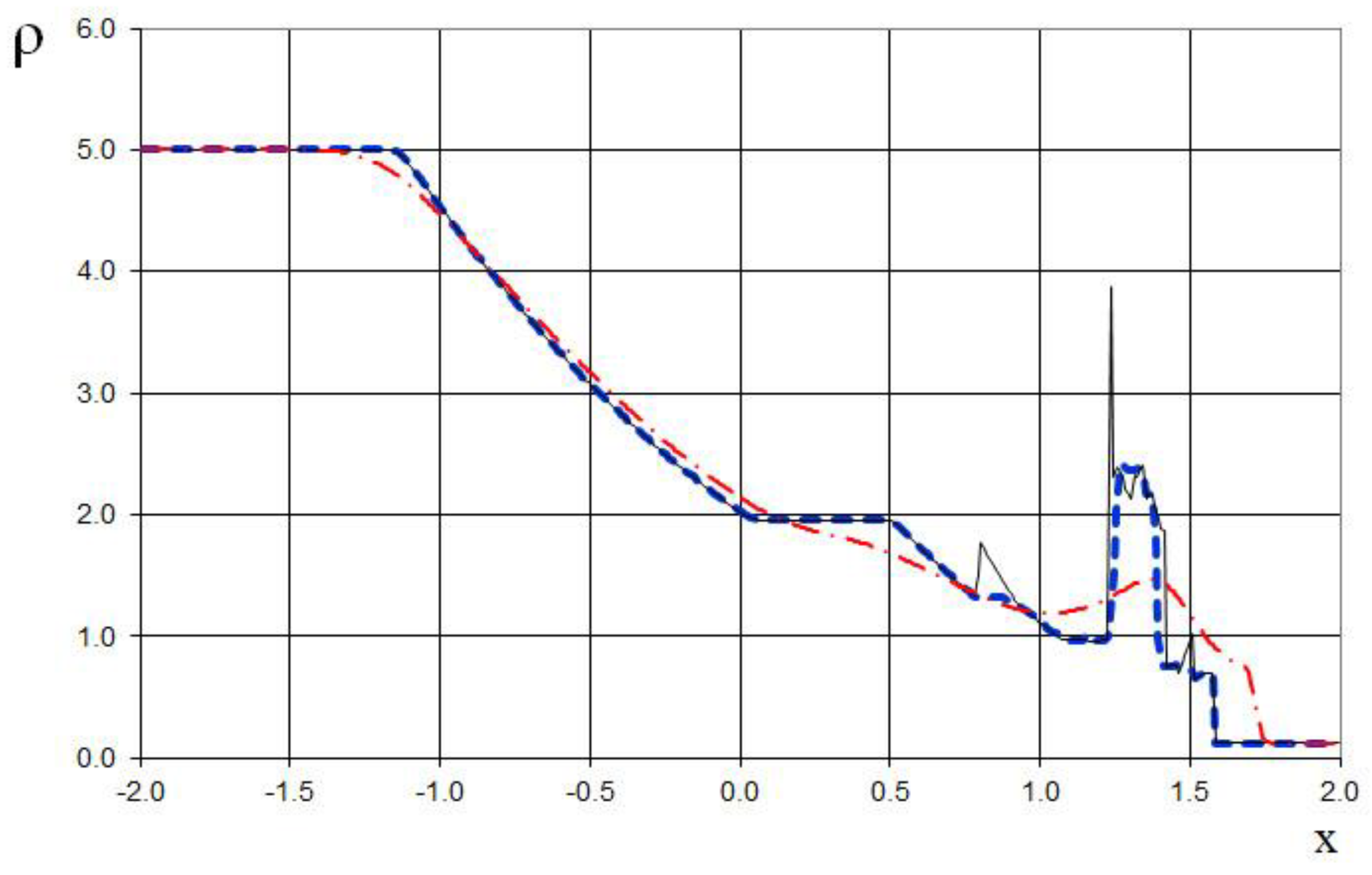
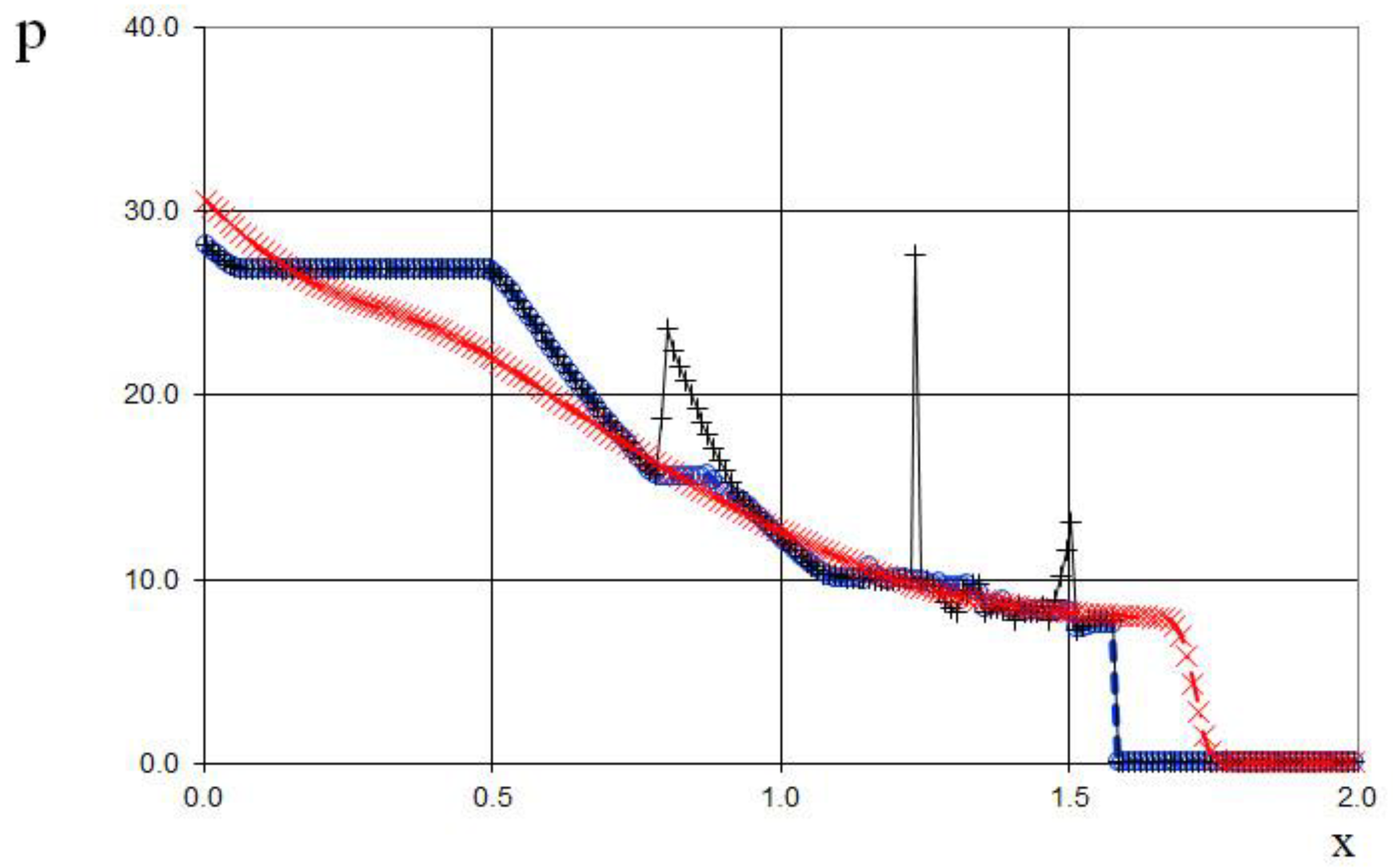
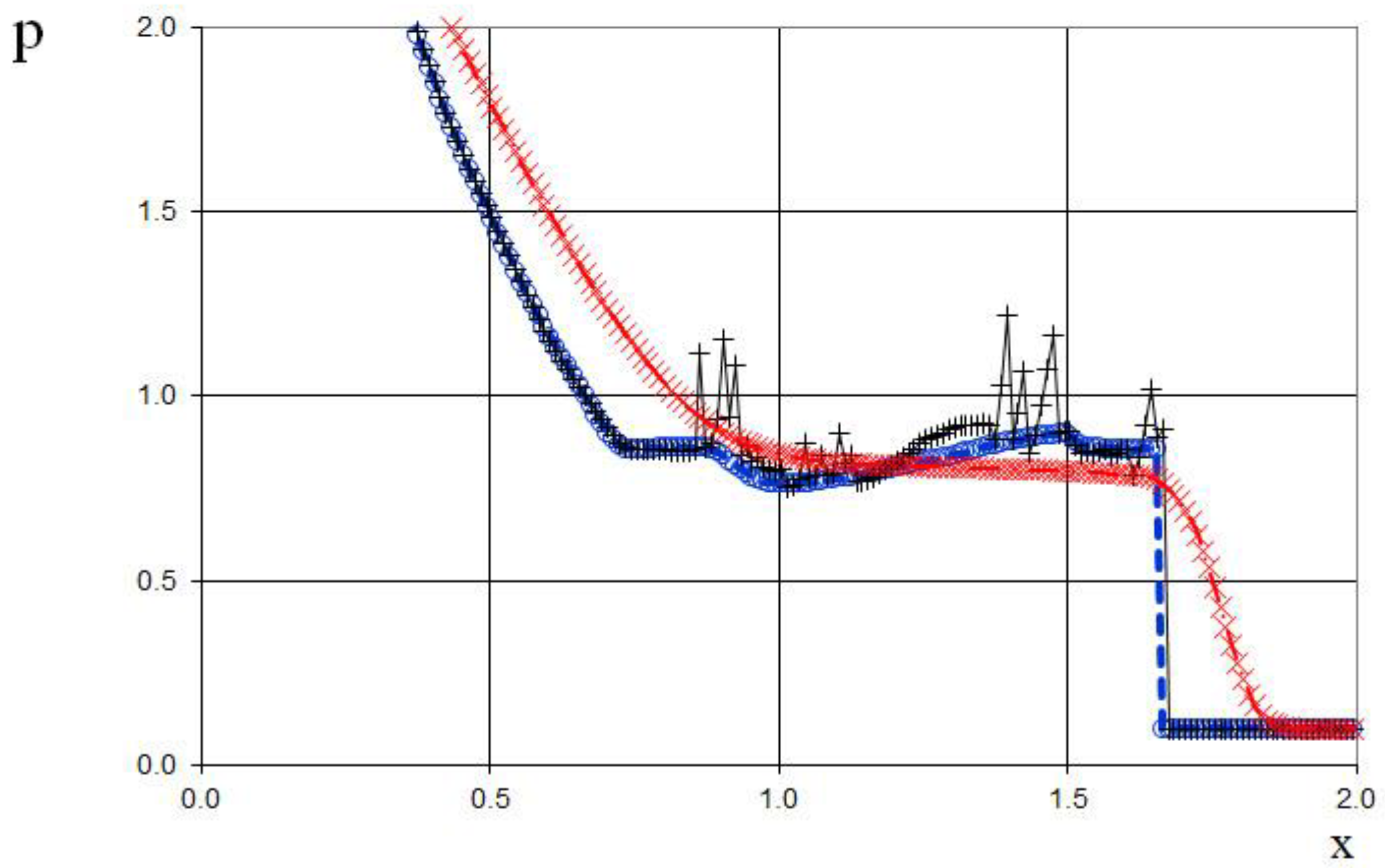
Figure 30.
Magnified view of density plot for the two Riemann problems interaction (65): the ULT1C scheme of Harten (red dash dotted line), the previous method [19] (black solid line), and the present method (blue dashed line).
Figure 30.
Magnified view of density plot for the two Riemann problems interaction (65): the ULT1C scheme of Harten (red dash dotted line), the previous method [19] (black solid line), and the present method (blue dashed line).
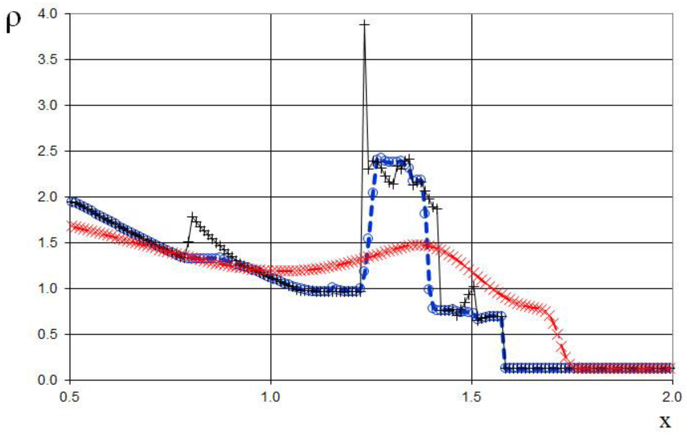
Figure 31.
Velocity plot for the two Riemann problems interaction (65): the ULT1C scheme of Harten (red dash dotted line), the previous method [19] (black solid line), and the present method (blue dashed line).
Figure 31.
Velocity plot for the two Riemann problems interaction (65): the ULT1C scheme of Harten (red dash dotted line), the previous method [19] (black solid line), and the present method (blue dashed line).
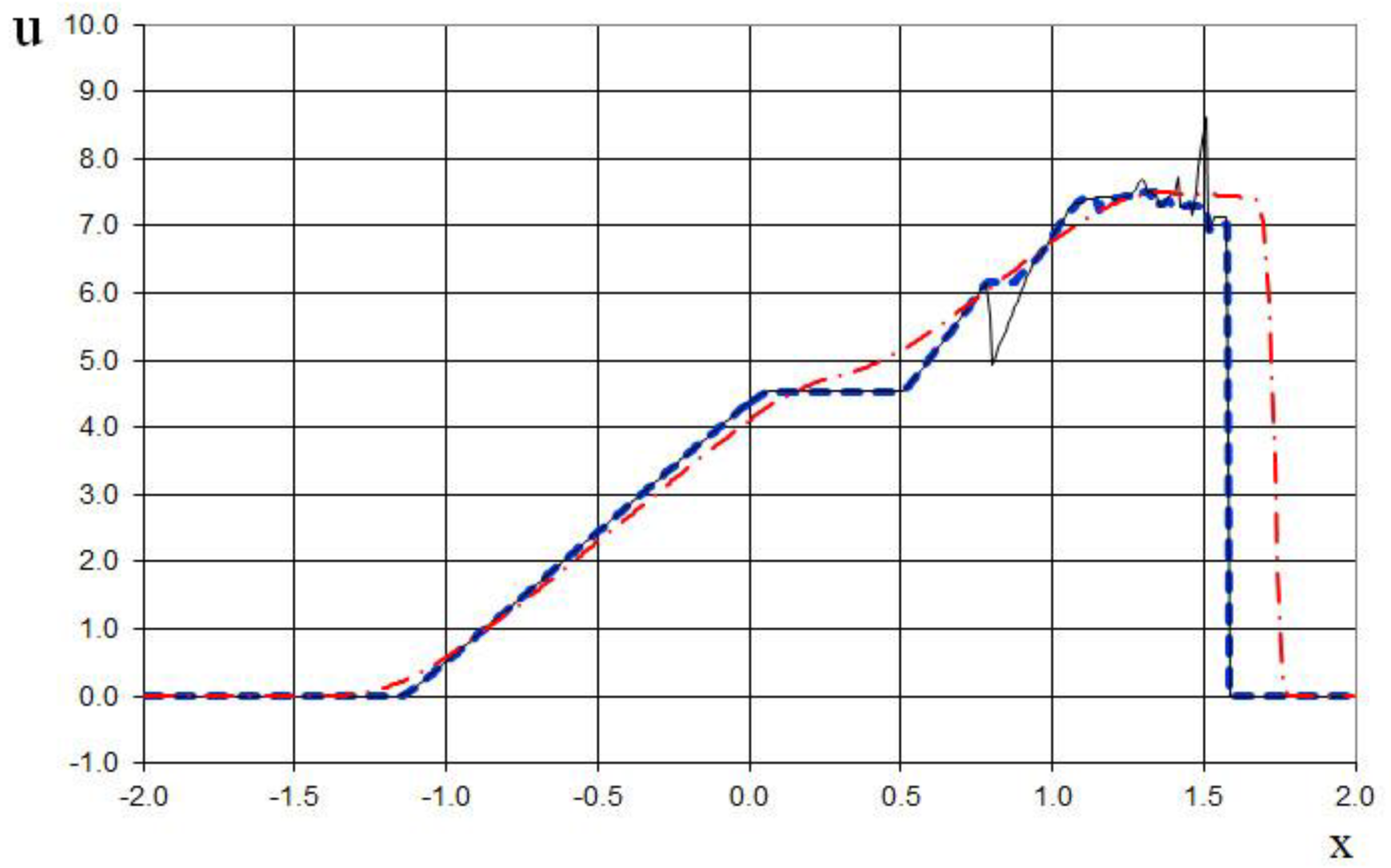
Figure 32.
Magnified view of velocity plot for the two Riemann problems interaction (65): the ULT1C scheme of Harten (red dash dotted line), the previous method [19] (black solid line), and the present method (blue dashed line).
Figure 32.
Magnified view of velocity plot for the two Riemann problems interaction (65): the ULT1C scheme of Harten (red dash dotted line), the previous method [19] (black solid line), and the present method (blue dashed line).
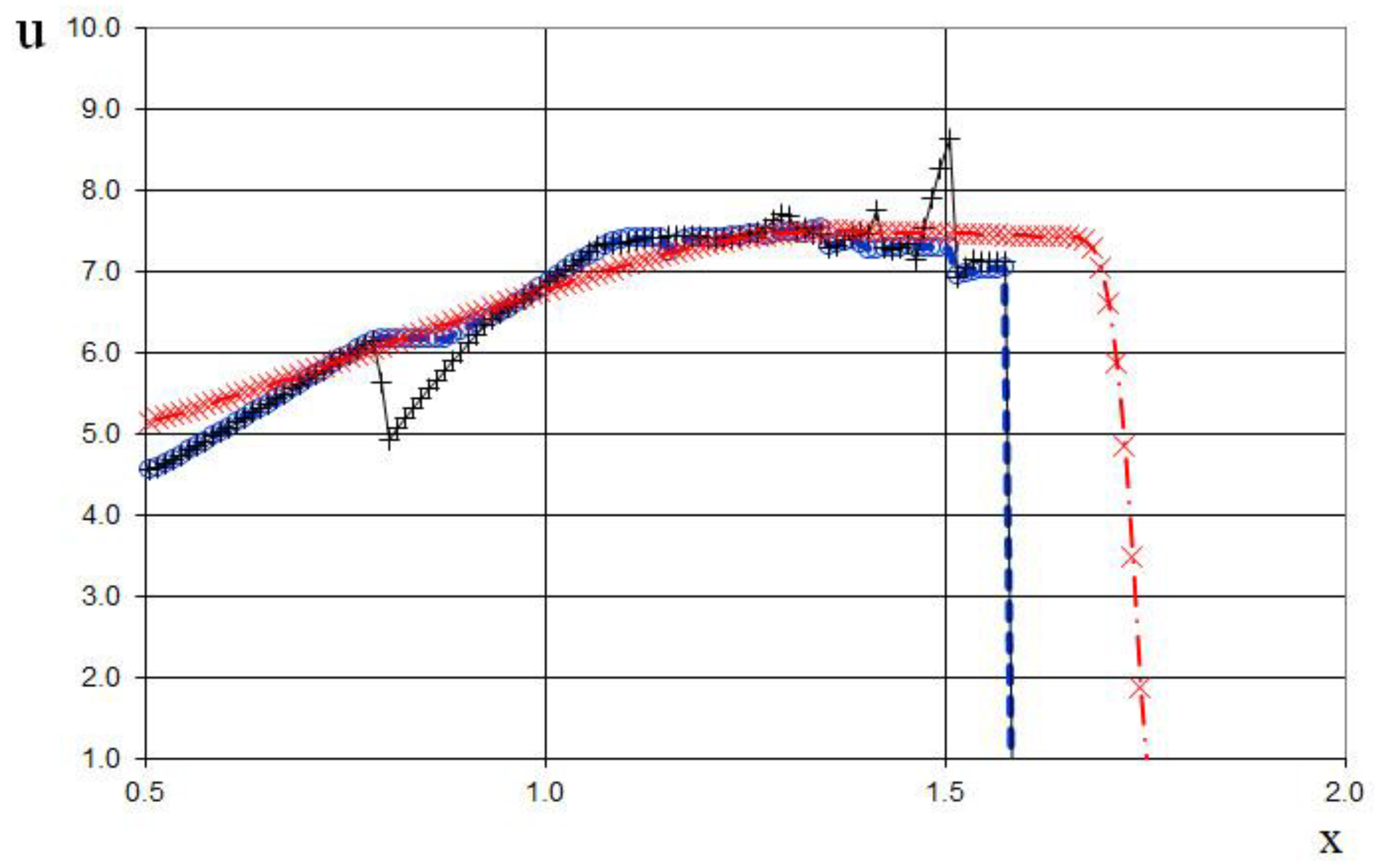
Figure 33.
Pressure plot for the two Riemann problems interaction (65): the ULT1C scheme of Harten (red dash dotted line), the previous method [19] (black solid line), and the present method (blue dashed line).
Figure 33.
Pressure plot for the two Riemann problems interaction (65): the ULT1C scheme of Harten (red dash dotted line), the previous method [19] (black solid line), and the present method (blue dashed line).
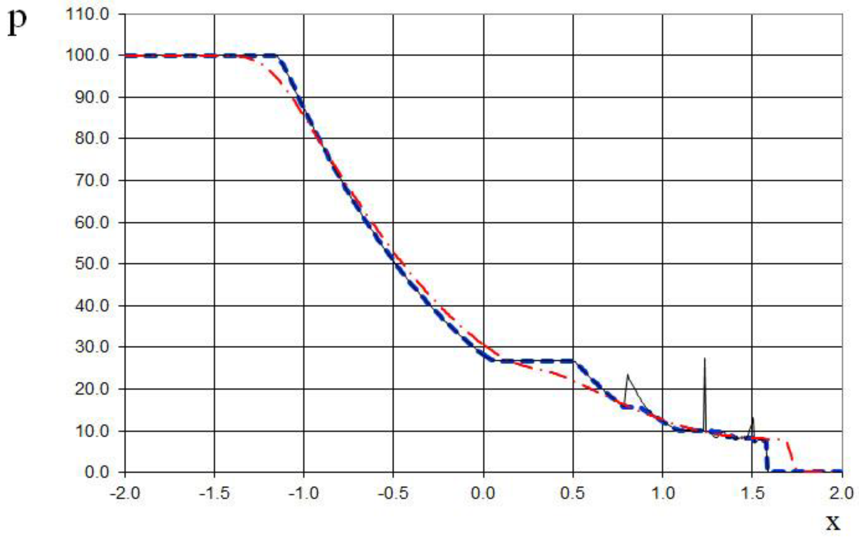
Figure 34.
Magnified view of pressure plot for the two Riemann problems interaction (65): the ULT1C scheme of Harten (red dash dotted line), the previous method [19] (black solid line), and the present method (blue dashed line).
Figure 34.
Magnified view of pressure plot for the two Riemann problems interaction (65): the ULT1C scheme of Harten (red dash dotted line), the previous method [19] (black solid line), and the present method (blue dashed line).
4. Discussion
The numerical solutions for the aforementioned well-known test cases were compared with the exact solutions, data from Harten’s method, and the results of the author's previous approach. The obtained results lead to the following conclusions:
(1) The primary advantage of the proposed method over the well-known TVD, ENO, and WENO methods is the elimination of the numerical viscosity (diffusion) for shocks;
(2) Over time, shocks or rarefaction waves may spread slightly slower or faster than in the exact solution. This discrepancy arises from rounding the wave front positions to the grid cell accuracy, a consequence of using a fixed homogeneous grid.
(3) The proposed scheme allows us to obtain more universal and accurate results than the previous method [19], and it has no sawtooth oscillations.
The accuracy of the proposed method for handling flow discontinuities is determined by the iterative Godunov exact solver. In the calculations, an iteration termination criterion of less than 10-5 is used to ensure convergence by measuring the pressure difference between consecutive iterations.
The directions for further research are connected with one-dimensional, two-dimensional Sedov problem modeling and two-dimensional Riemann problem simulations.
Funding
This research did not receive any specific grant from funding agencies in the public, commercial, or not-for-profit sectors.
Acknowledgments
I am grateful to Professor V.G. Shakhov and other anonymous referees for their insightful comments and advice, which have greatly improved the quality of this work.
Conflicts of Interest
The author declares no conflict of interest.
Nomenclature
| Symbol | Meaning |
| Convective velocity of flow | |
| Direction | |
| Time | |
| Time step, marching time step | |
| Tolerance associated with the comparison of the flow variables | |
| Machine arithmetic tolerance associated with the comparison of the coordinates | |
| Grid step | |
| Number of grid cells | |
| Convective velocity of a shock | |
| Integer coefficient in the formula for the time step at the convection stage | |
| Left boundary of a modeling area | |
| Right boundary of the modeling area | |
| Density | |
| Pressure | |
| Ratio of specific heat coefficients | |
| Sound velocity | |
| Transfer variables of wave equations | |
| Transfer vector variables | |
| Coordinate index | |
| Coordinate index | |
| Time index | |
| Pressure function for adiabatic law | |
| time step at the acoustics stage | |
| Acoustic velocity of a shock | |
| Integer coefficient in the formula for the time step at the acoustics stage | |
| Time step at the convection stage | |
| An integer showing how many times the time step at the acoustics stage is greater than the marching time step | |
| An integer showing how many times the time step at the convection stage is greater than the marching time step | |
| Internal specific energy | |
| Jacobian matrix | |
| Diagonal matrix of eigenvalues of the Jacobian matrix | |
| Matrix of corresponding left eigenvectors | |
| Matrix of corresponding right eigenvectors | |
| Diagonal identity matrix | |
| Constant sound velocity | |
| Constant density | |
| Density of the exact solution of the Riemann problem on the left | |
| Density of the exact solution of the Riemann problem on the right | |
| Velocity of the exact solution of the Riemann problem on the left | |
| Velocity of the exact solution of the Riemann problem on the right | |
| Internal specific energy of the Riemann problem on the left | |
| Internal specific energy of the Riemann problem on the right | |
| Pressure of the Riemann problem on the left | |
| Pressure of the Riemann problem on the right | |
| Velocity of the propagation of a shock or rarefaction wave of the Riemann problem on the left | |
| Velocity of the propagation of a shock or rarefaction wave of the Riemann problem on the right | |
| Local acoustic velocity of the Riemann problem on the left | |
| Local acoustic velocity of the Riemann problem on the right | |
| Density after the acoustics stage | |
| Pressure after the acoustics stage | |
| Velocity after the acoustics stage | |
| Internal specific energy after the acoustics stage | |
| Density after the convection stage | |
| Pressure after the convection stage | |
| Velocity after the convection stage | |
| Internal specific energy after the convection stage | |
| Velocity on the right | |
| Density for the initial conditions | |
| Pressure for the initial conditions | |
| Velocity for the initial conditions | |
| Pi |
References
- von Neumann J.; Richtmyer, R.D. A method for the numerical calculation of hydrodynamic shocks. J. Appl. Phys. 1950, 21, 232.
- Jameson, A. Analysis and design of numerical schemes for gas dynamics, 1: artificial diffusion, upwind biasing, limiters and their effect on accuracy and multigrid convergence. Int. J. Comput. Fluid Dyn. 1994, 4, 171–218.
- Harten, A. A high resolution scheme for the computation of weak solutions of hyperbolic conservation laws. J. Comput. Phys. 1983, 49, 357–393.
- Harten, A.; Engquist, B.; Osher, S.; Chakravarthy, S.R. Uniform high order accurate essentially non-oscillatory schemes, III. J. Comput. Phys. 1987, 71, 231–303.
- Liu, X.D.; Osher, S.; Chan, T. Weighted essentially non-oscillatory schemes. J. Comput. Phys. 1994, 115, 200–212.
- Harten, A. ENO schemes with subcell resolution. J. Comput. Phys. 1987, 83, 148–184.
- Harten, A.; Osher, S. Uniformly high order essentially non-oscillatory schemes I. SIAM J. Numer. Anal. 1987, 24, 279–309.
- Harten, A.; Osher, S.; Engquist, B.; Chakravarthy, S. Some results on uniformly high order accurate essentially non-oscillatory schemes. Appl. Numer. Math. 1986, 2, 347–377.
- Shu, C.-W.; Osher, S. Efficient implementation of essentially non-oscillatory shock-capturing schemes. J. Comput. Phys. 1988, 77, 439–471.
- Shu, C.-W.; Osher, S. Efficient implementation of essentially non-oscillatory shock-capturing schemes II. J. Comput. Phys. 1989, 83, 32–78.
- Jiang, G.-S.; Shu, C.-W. Efficient implementation of Weighted ENO schemes. J. Comput. Phys. 1996, 126, 202–228.
- Pawar, S.; San, O. CFD Julia: A Learning Module Structuring an Introductory Course on Computational Fluid Dynamics. Fluids, 2019, 4, P. 159. [CrossRef]
- Roe, P.L. Approximate Riemann solvers, parameter vectors, and difference schemes. J. Comput. Phys. 1997, 135, 250-258.
- Godunov, S.K. A difference scheme for numerical computation of discontinuous solution of hyperbolic equation, Mat. Sbornik 1959, 47, 271–306.
- LeVeque, R.J. Balancing source terms and flux gradients on high-resolution Godunov methods: the quasi-steady wave-propagation algorithm. J. Comput. Phys. 1998, 146, 346–365.
- Einfeldt, B. On Godunov-type methods for gas dynamics. SIAM Journal on Numerical Analysis. 1988, 25(2), 294–318.
- Wu, Y.Y.; Cheung, K.F. Explicit solution to the exact Riemann problem and application in nonlinear shallow-water equations. Int. J. Numer. Meth. Fluids. 2008, 57(11), 1649–1668. Bibcode:2008IJNMF..57.1649W. [CrossRef]
- Saba Basiri, Seyyed Mohammad Ghoreishi, Jaber Safdari, Sadegh Yousefi-Nasab, Three-dimensional simulation of gas flow for predicting the pressure and velocity profiles inside a gas centrifuge machine using the DSMC method. Vacuum. 2024, 219, Part A, P. 112664, ISSN 0042-207X. [CrossRef]
- Nikonov, V. A Semi-Lagrangian Godunov-Type Method without Numerical Viscosity for Shocks. Fluids. 2022, 7, P. 16. [CrossRef]
- Taylor, E.M.; Wu, M.; Martin, M.P. Optimization of Nonlinear Error for Weighted Essentially Non-Oscillatory Methods in Direct Numerical Simulations of Compressible Turbulence. J. Comput. Phys. 2007, 223, 384-397.
- Sod, G.A. A survey of several finite difference methods for systems of nonlinear hyperbolic conservation laws. J. Comput. Phys. 1978, 107, 1–31.
- Lax, P.D. Weak solutions of nonlinear hyperbolic equations and their numerical computation. Commun. Pure Appl. Math. 1954, 7, 159–193.
- Carmouze, Q.; Saurel, R.; Chiapolino, A.; Lapebie, E. Riemann solver with internal reconstruction (RSIR) for compressible single-phase and non-equilibrium two-phase flows. J. Comput. Phys. 2020, 408, 109-176.
- Feng, H.; Hu, F.; Wang, R. A New Mapped Weighted Essentially Non-oscillatory Scheme. J. Sci. Comput. 2012, 51, 449–473. [CrossRef]
- Fu, L.; Xiangyu, Y.H.; Nikolaus A.A. A new class of adaptive high-order targeted ENO schemes for hyperbolic conservation laws. J. Comput. Phys. 2018, 374, 724–751.
Figure 1.
Initial conditions prior to solving the three Riemann problems.
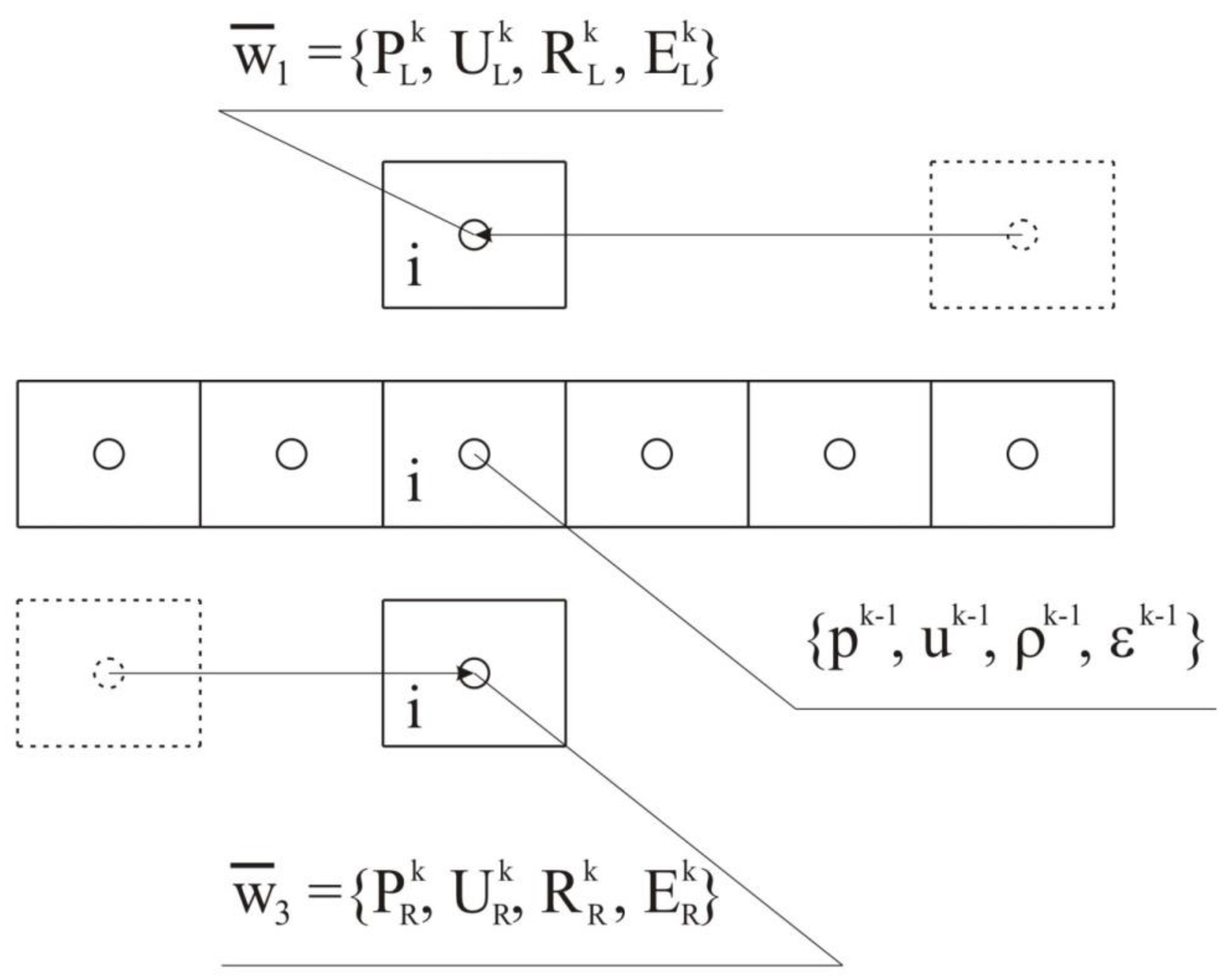
Figure 2.
The first Riemann problem.
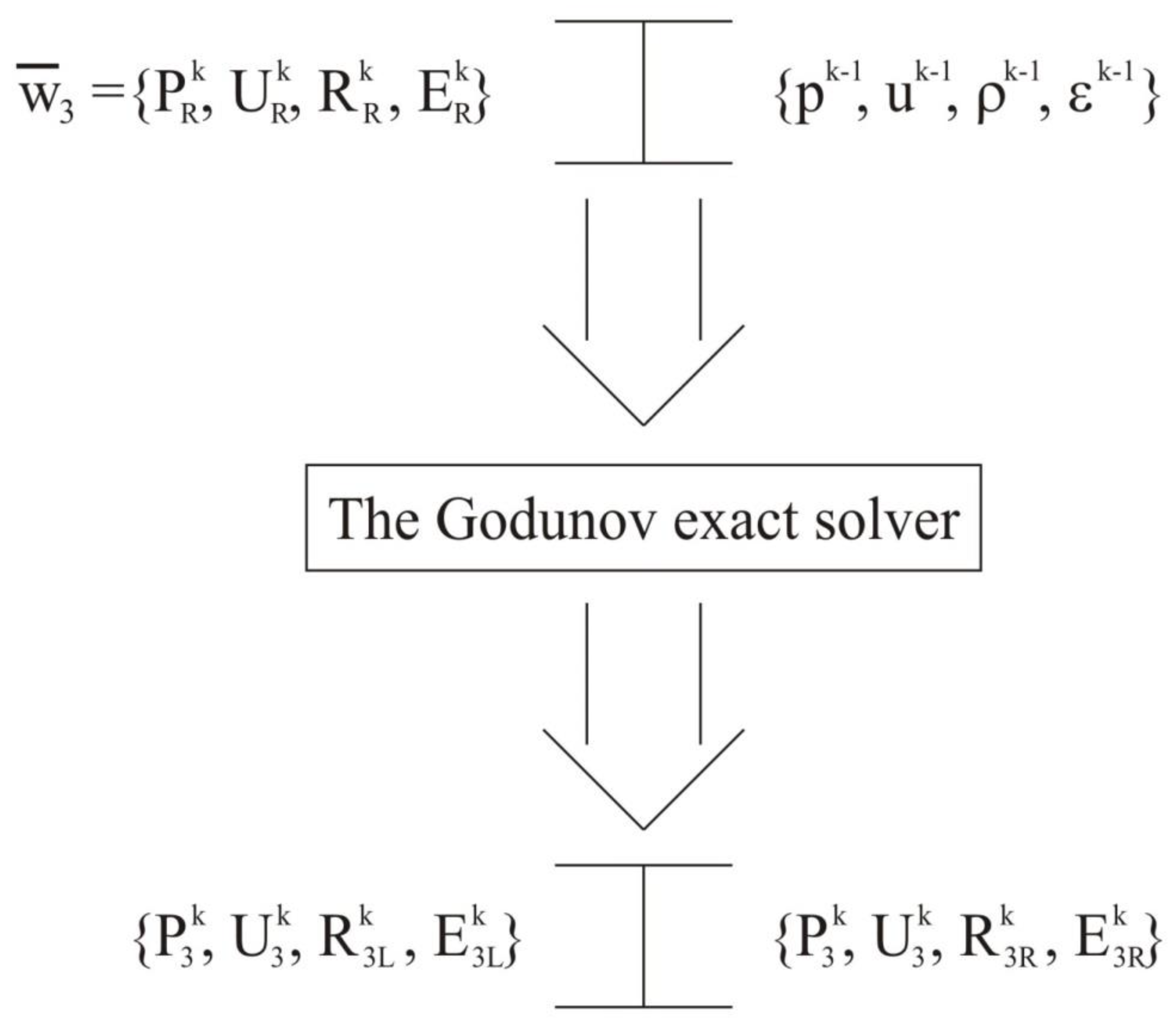
Figure 3.
The second Riemann problem.
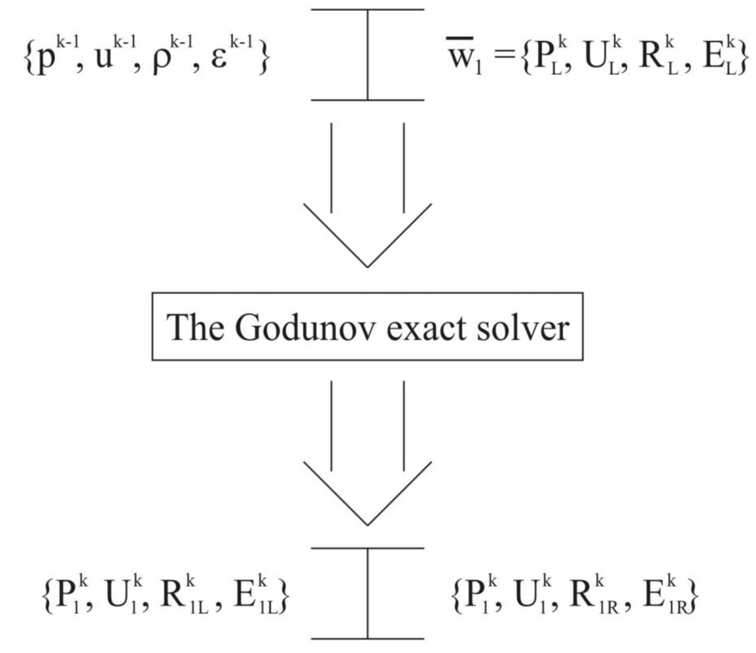
Figure 4.
The third Riemann problem.
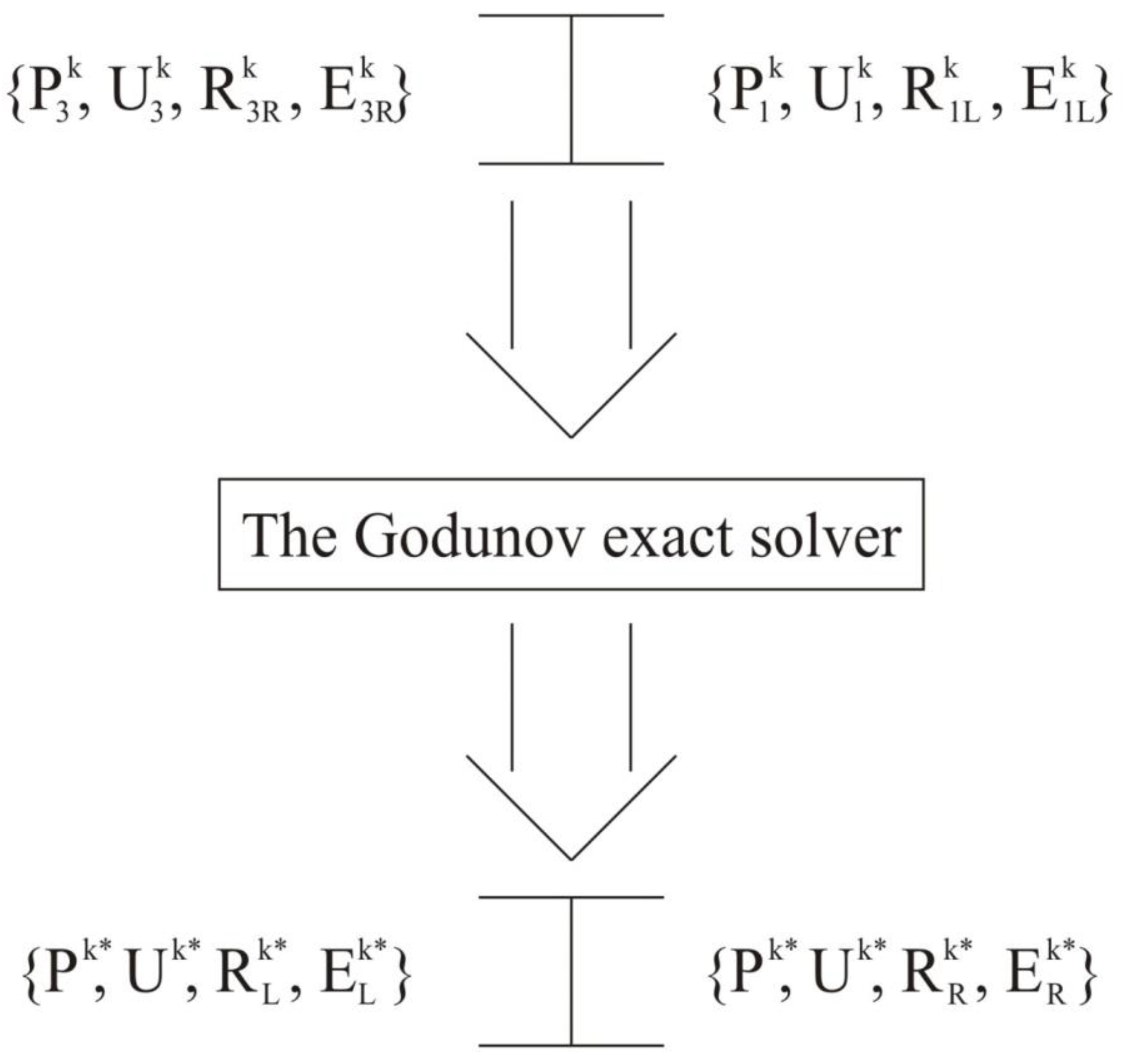
Figure 5.
Density plot for the shock-tube problem of Sod: the exact solution (line), the previous method [19] (cross), and the present method (circle).
Figure 5.
Density plot for the shock-tube problem of Sod: the exact solution (line), the previous method [19] (cross), and the present method (circle).
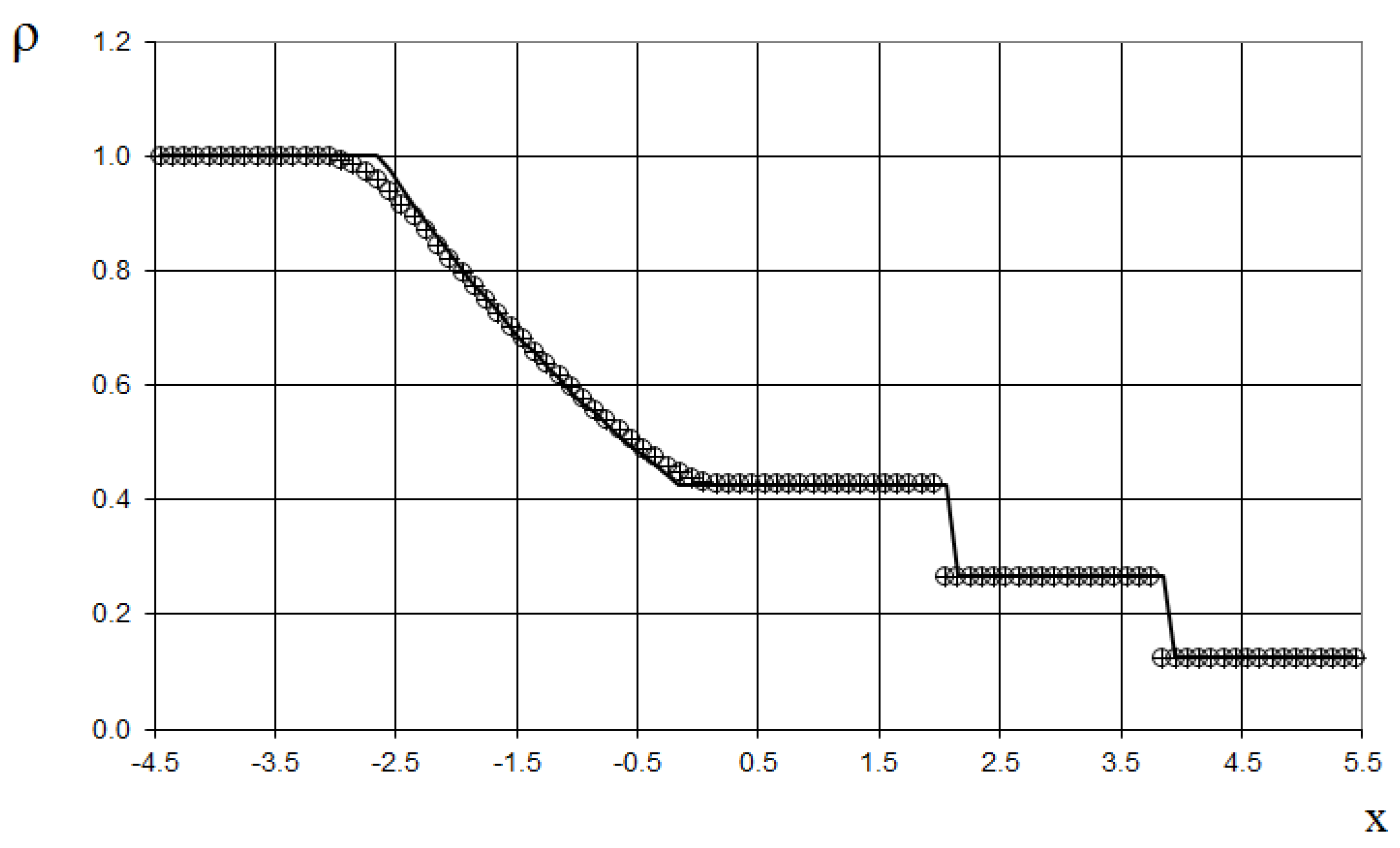
Figure 6.
Velocity plot for the shock-tube problem of Sod: the exact solution (line), the previous method [19] (cross), and the present method (circle).
Figure 6.
Velocity plot for the shock-tube problem of Sod: the exact solution (line), the previous method [19] (cross), and the present method (circle).
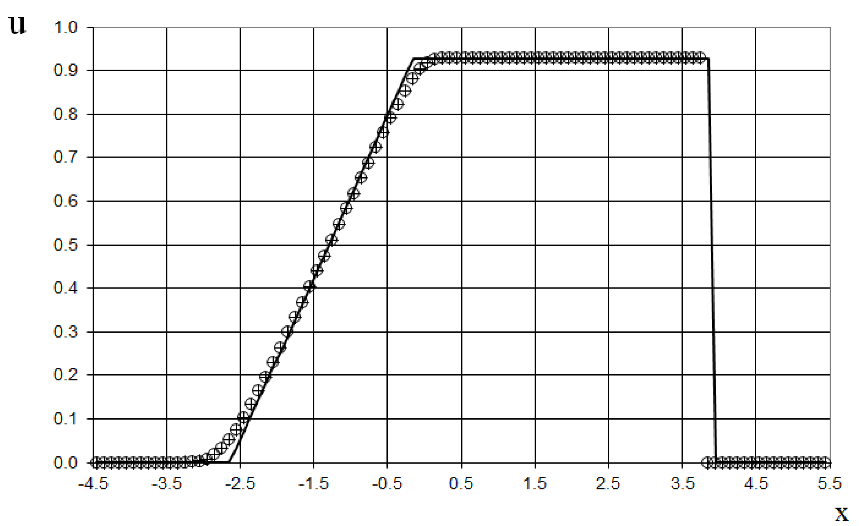
Figure 7.
Pressure plot for the shock-tube problem of Sod: the exact solution (line), the previous method [19] (cross), and the present method (circle).
Figure 7.
Pressure plot for the shock-tube problem of Sod: the exact solution (line), the previous method [19] (cross), and the present method (circle).
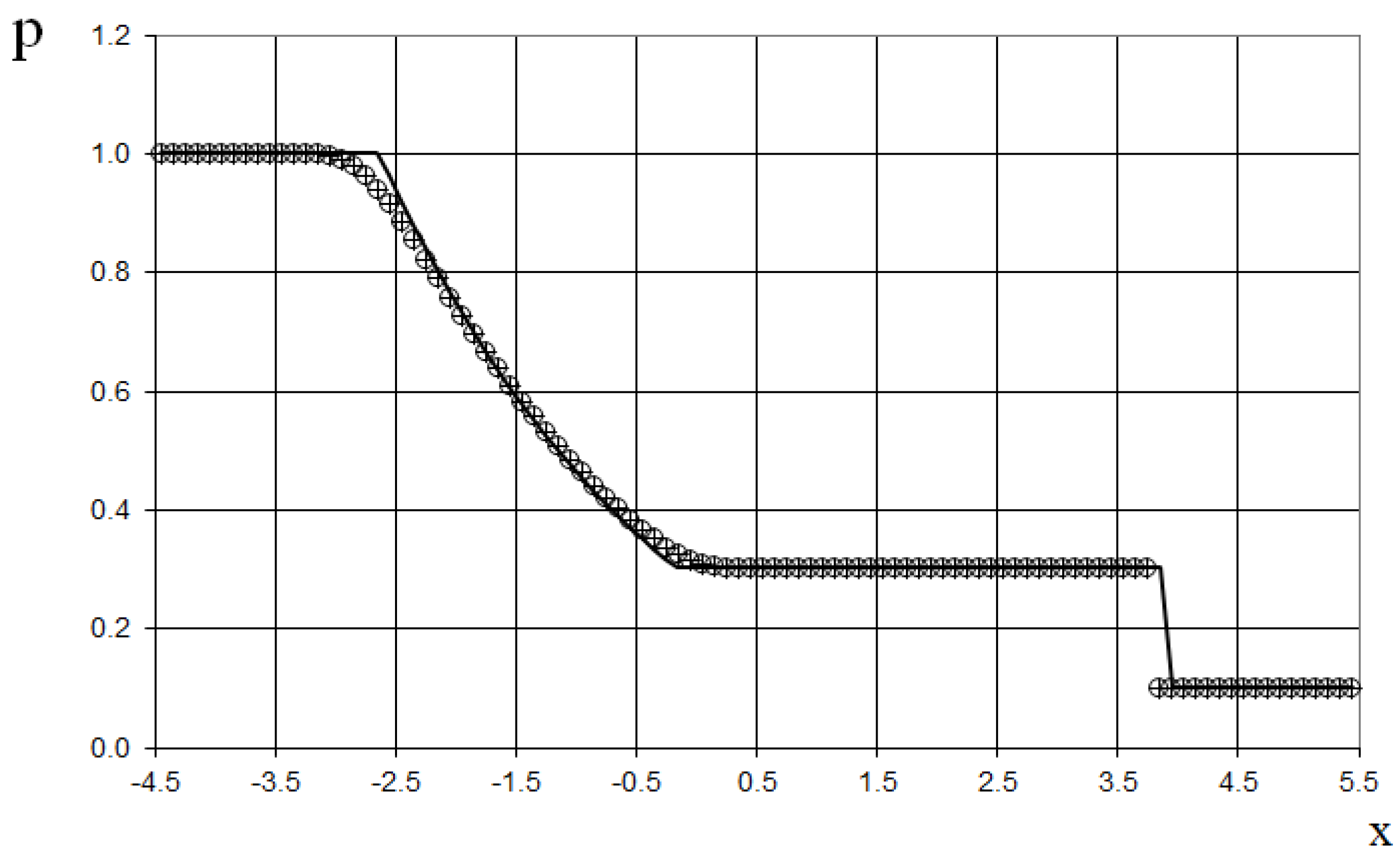
Figure 8.
Density plot for the Riemann problem of Lax: the exact solution (line), the previous method [19] (cross) , and the present method (circle).
Figure 8.
Density plot for the Riemann problem of Lax: the exact solution (line), the previous method [19] (cross) , and the present method (circle).
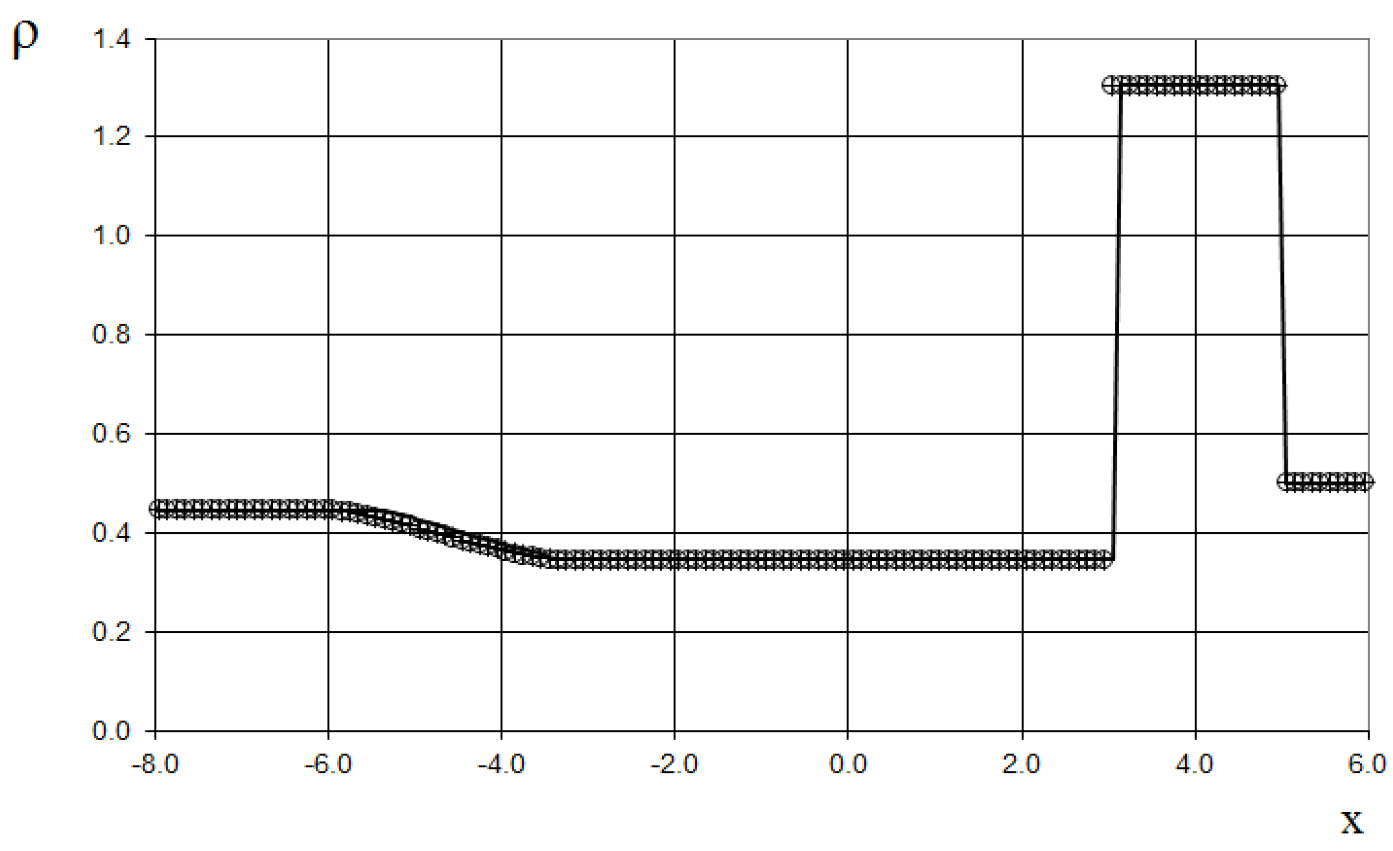
Figure 9.
Velocity plot for the Riemann problem of Lax: the exact solution (line), the previous method [19] (cross) , and the present method (circle).
Figure 9.
Velocity plot for the Riemann problem of Lax: the exact solution (line), the previous method [19] (cross) , and the present method (circle).
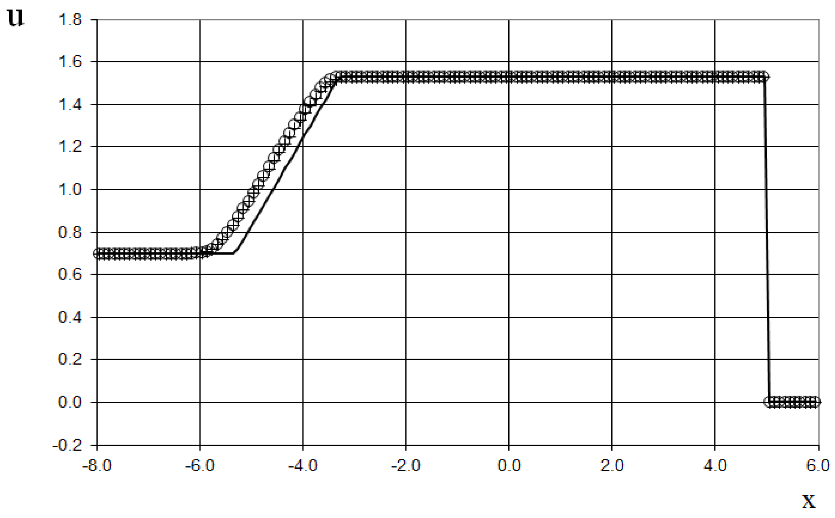
Figure 10.
Pressure plot for the Riemann problem of Lax: the exact solution (line), the previous method [19] (cross) , and the present method (circle).
Figure 10.
Pressure plot for the Riemann problem of Lax: the exact solution (line), the previous method [19] (cross) , and the present method (circle).
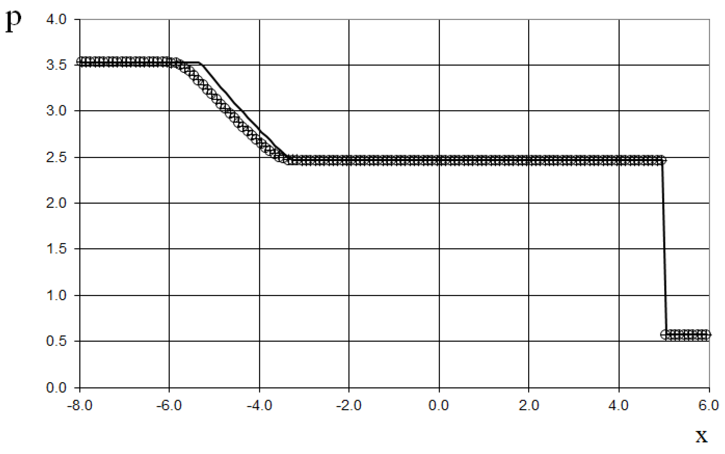
Figure 11.
Density plot for the Shu–Osher shock-tube problem (61), using the coarse grid (192 grid points): the “exact” solution [20] (line), the previous method [19] (cross), and the present method (circle).
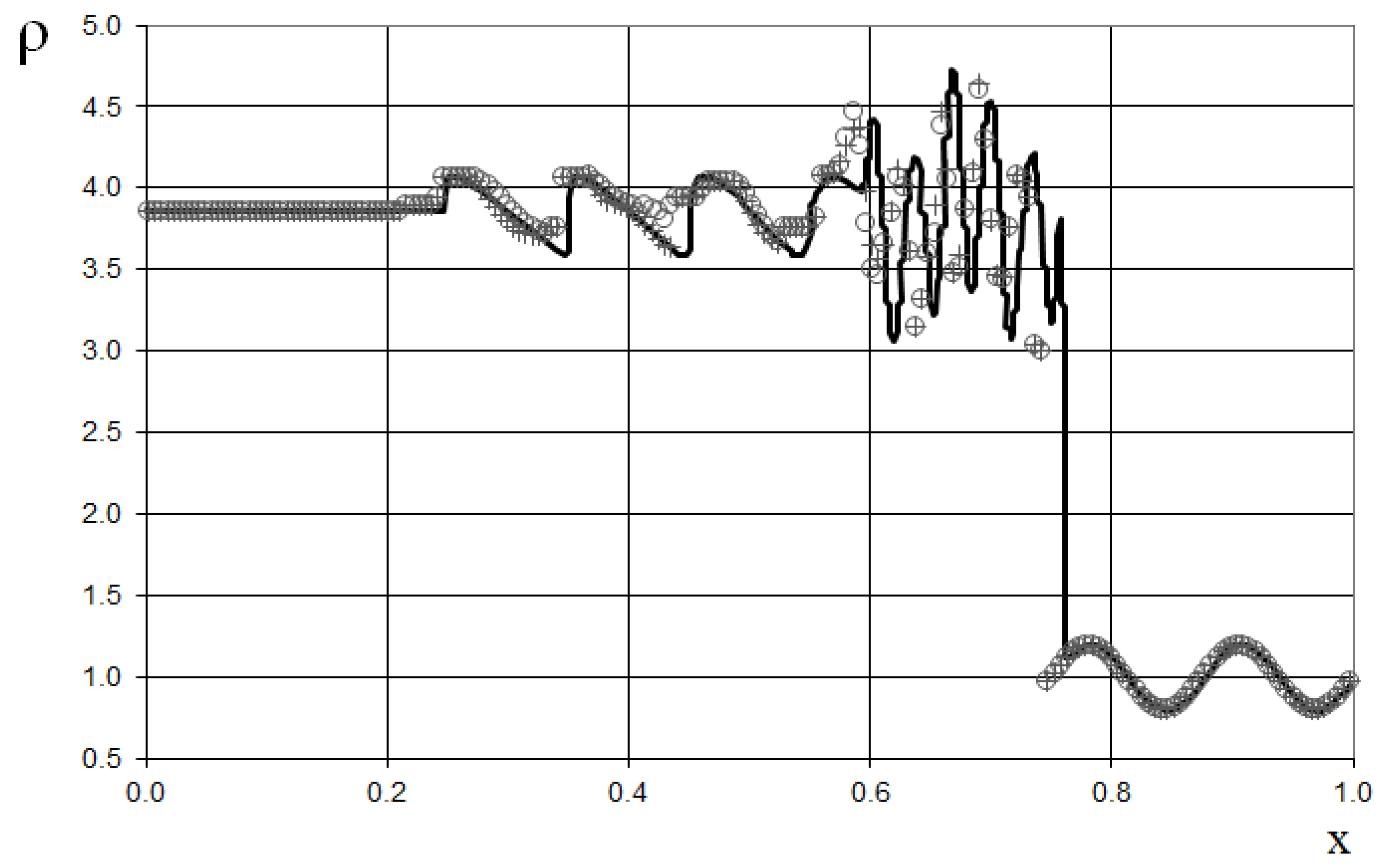
Figure 12.
Density plot for the Shu–Osher shock-tube problem, using the fine grid (384 grid points): the “exact” solution [20] (line), the previous method [19] (cross), and the present method (circle).
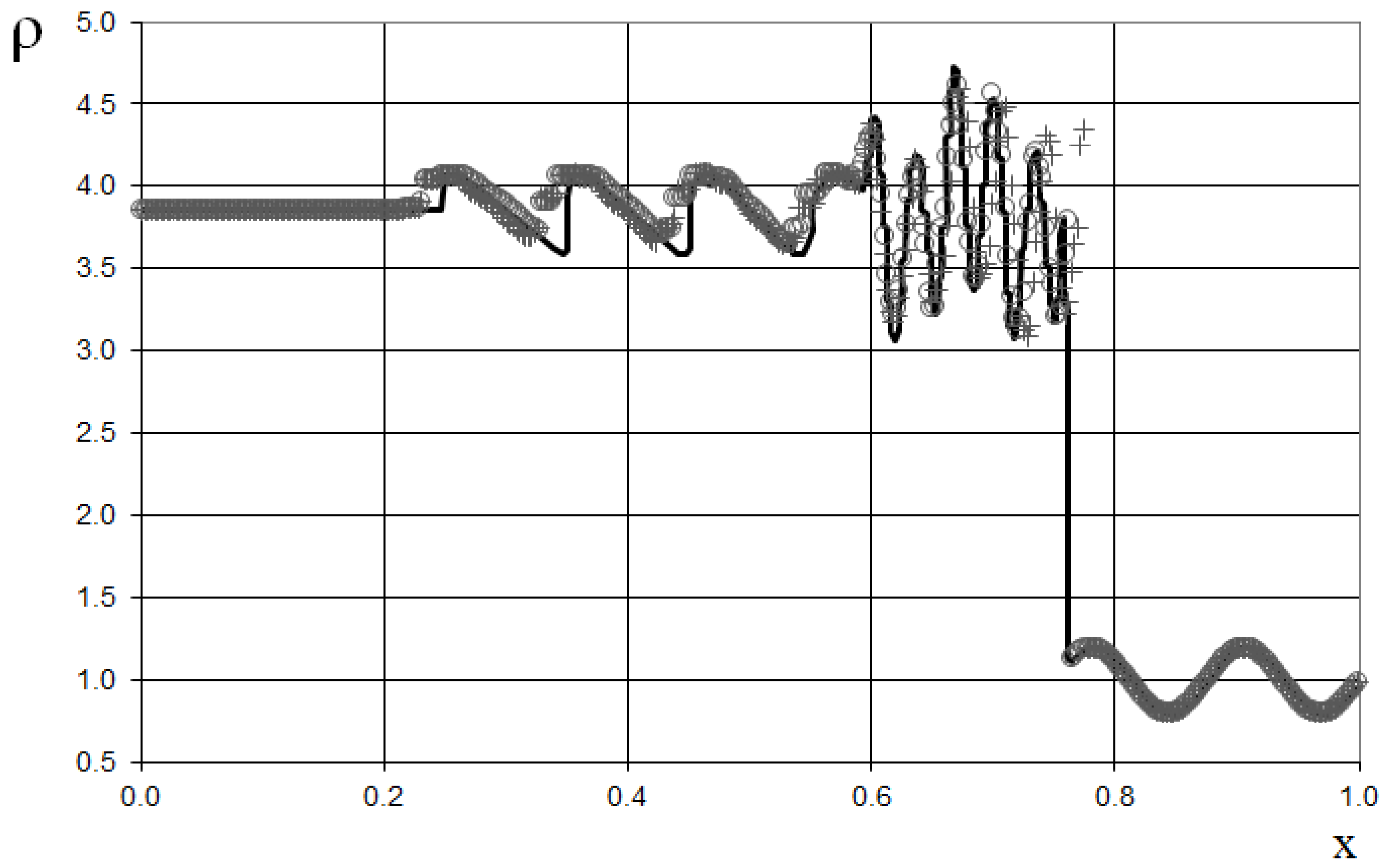
Figure 13.
Density plot for the Shu–Osher shock-tube problem, using the finer grid (1000 grid points): the “exact” solution [20] (line), the previous method [19] (cross), and the present method (circle).
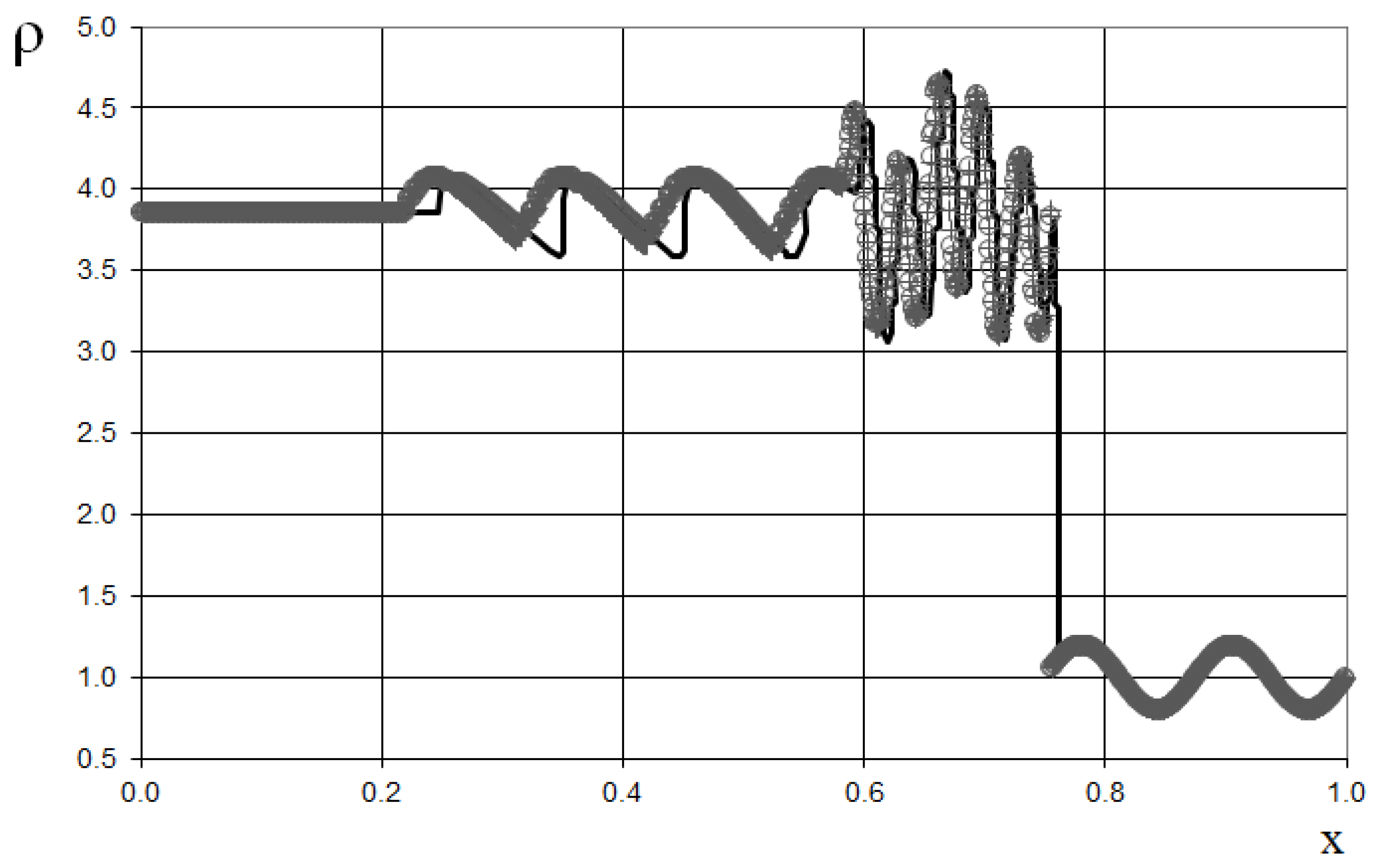
Figure 14.
Density plot for the double expansion wave problem (62) for the one-dimensional scalar hyperbolic conservation law, using the coarse grid (100 grid points): the exact solution [23] (line), the author's previous work method [19] (cross), and the present method (circle).
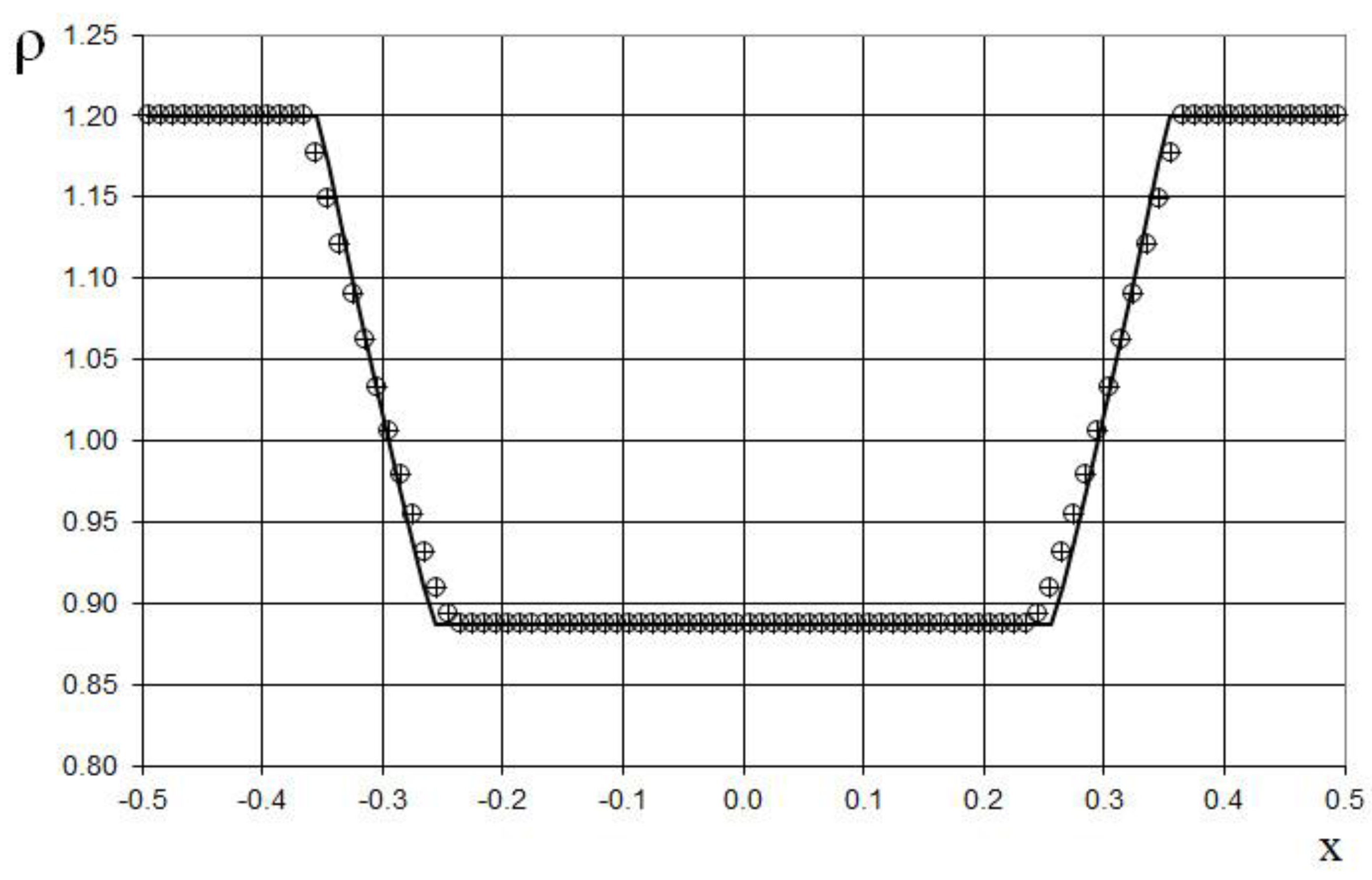
Figure 15.
Velocity plot for the double expansion wave problem (47) for the one-dimensional scalar hyperbolic conservation law, using the coarse grid (100 grid points): the exact solution [23] (line), the author's previous work method [19] (cross), and the present method (circle).
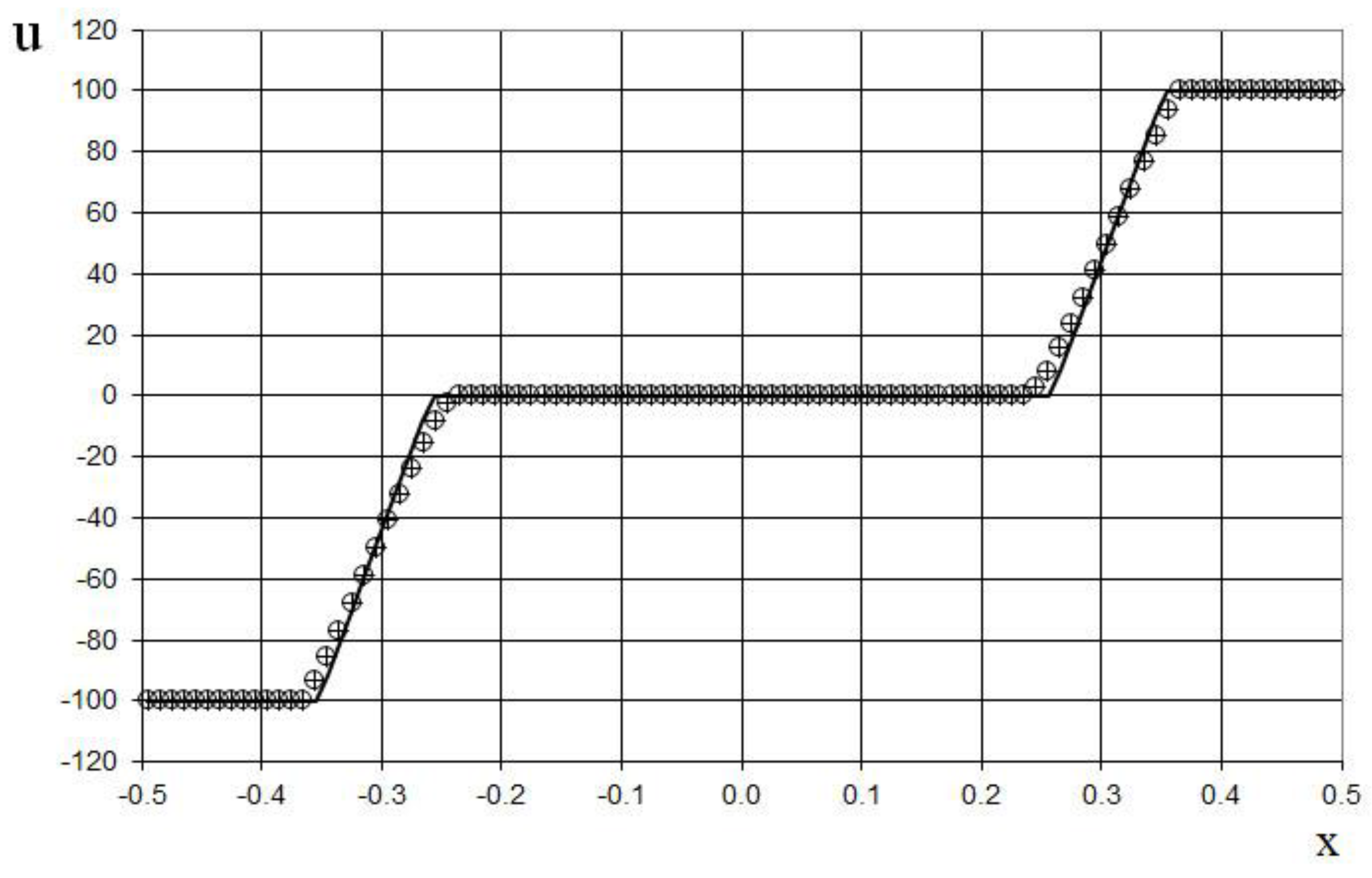
Figure 16.
Pressure plot for the double expansion wave problem (62) for the one-dimensional scalar hyperbolic conservation law, using the coarse grid (100 grid points): the exact solution [23] (line), the author's previous work method [19] (cross), and the present method (circle).
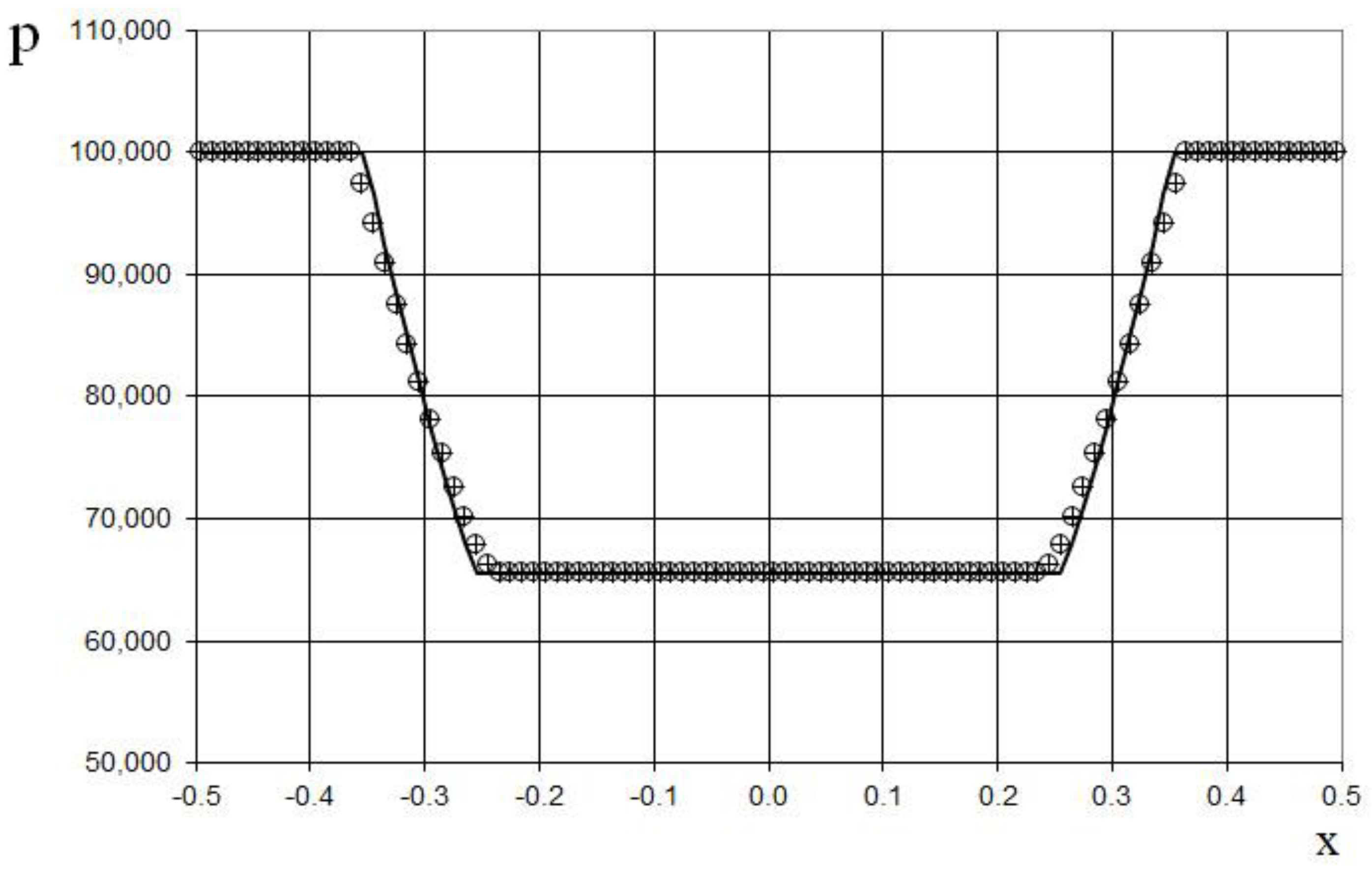
Figure 17.
Density plot for the double expansion wave problem (62) for the one-dimensional scalar hyperbolic conservation law, using the finer grid (1000 grid points): the exact solution [23] (black solid line), the author's previous work method [19] (black dotted line), and the present method (blue dashed line).
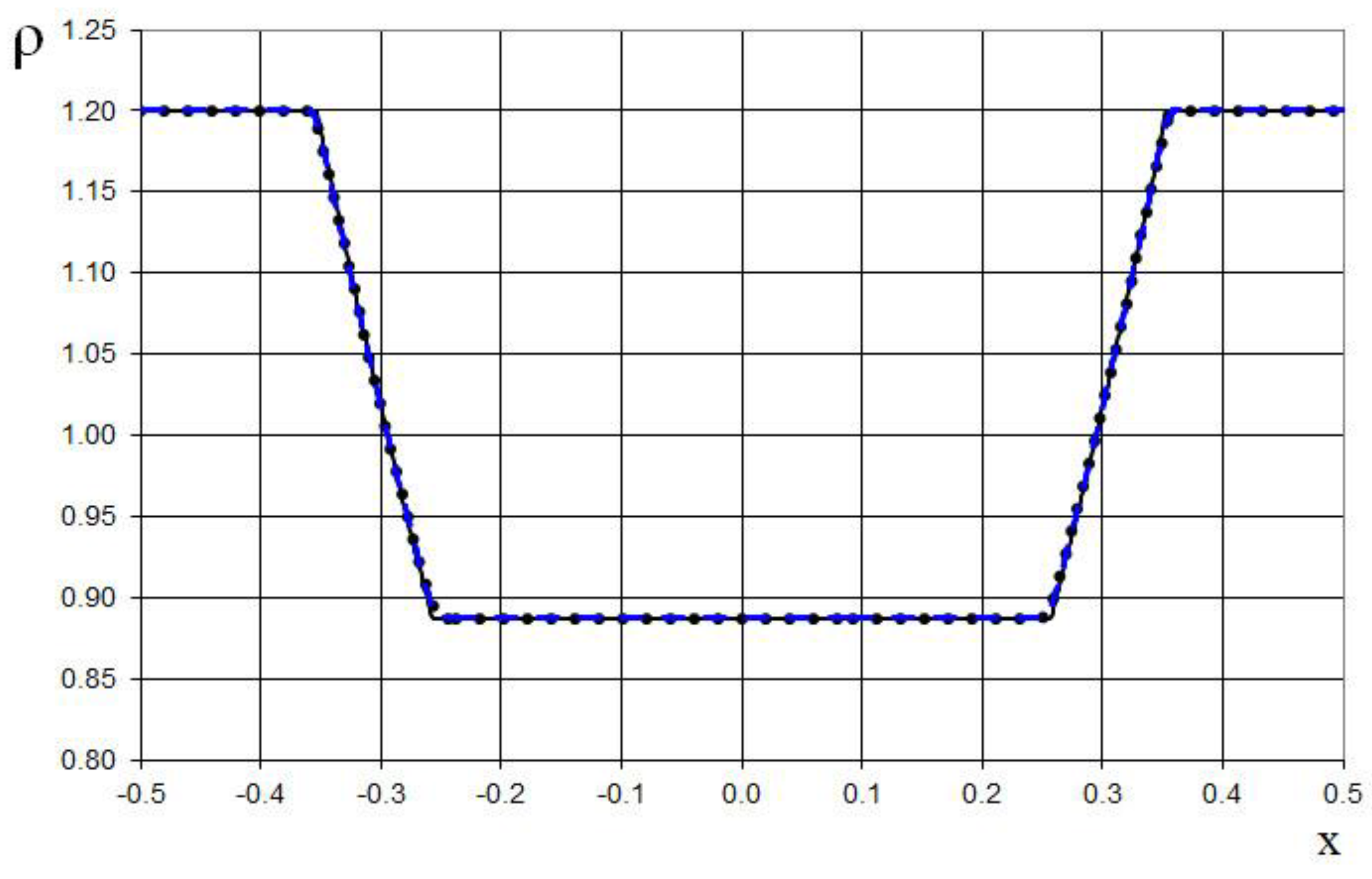
Figure 18.
Velocity plot for the double expansion wave problem (62) for the one-dimensional scalar hyperbolic conservation law, using the finer grid (1000 grid points): the exact solution [23] (black solid line), the author's previous work method [19] (black dotted line), and the present method (blue dashed line).
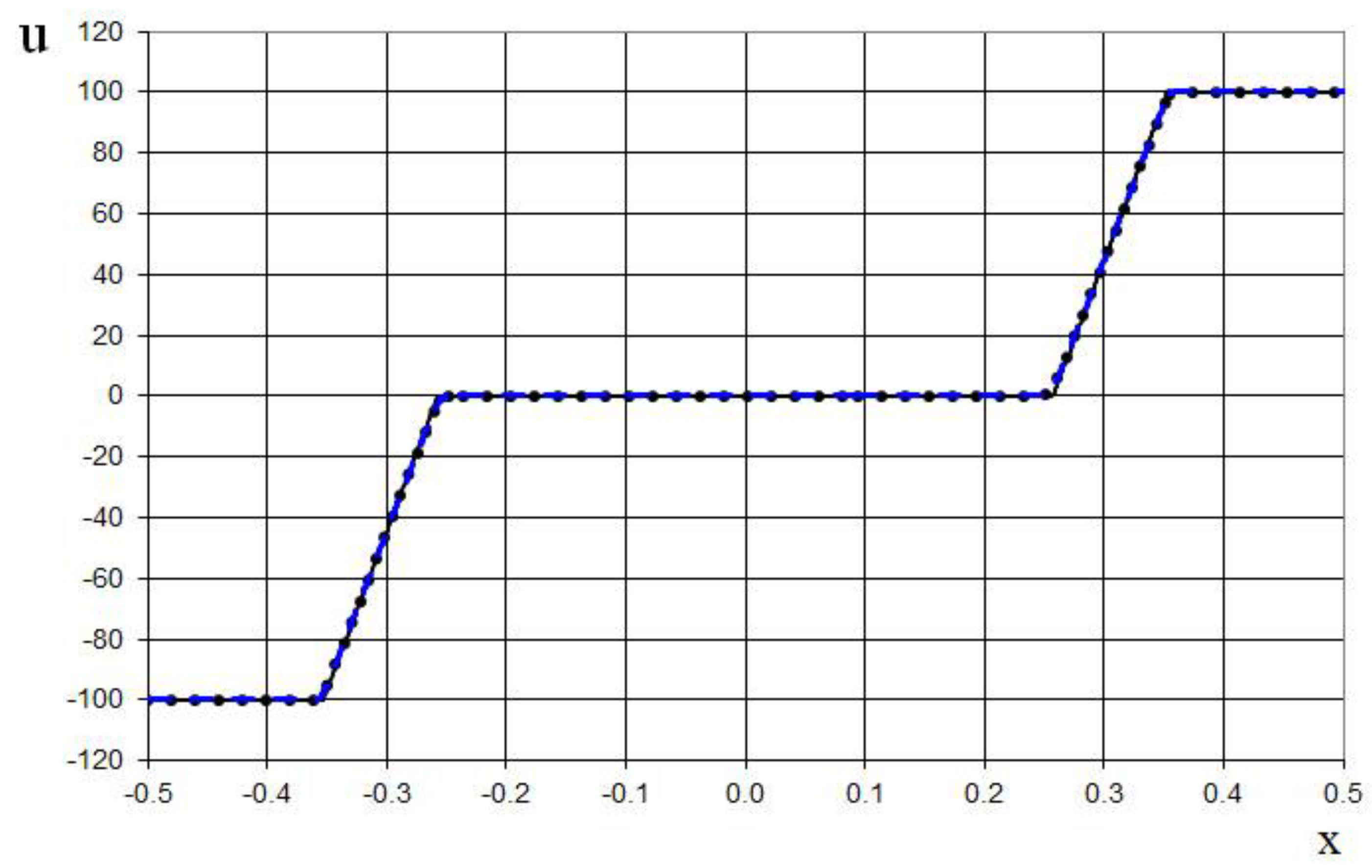
Figure 19.
Pressure plot for the double expansion wave problem (62) for the one-dimensional scalar hyperbolic conservation law, using the finer grid (1000 grid points): the exact solution [23] (black solid line), the author's previous work method [19] (black dotted line), and the present method (blue dashed line).
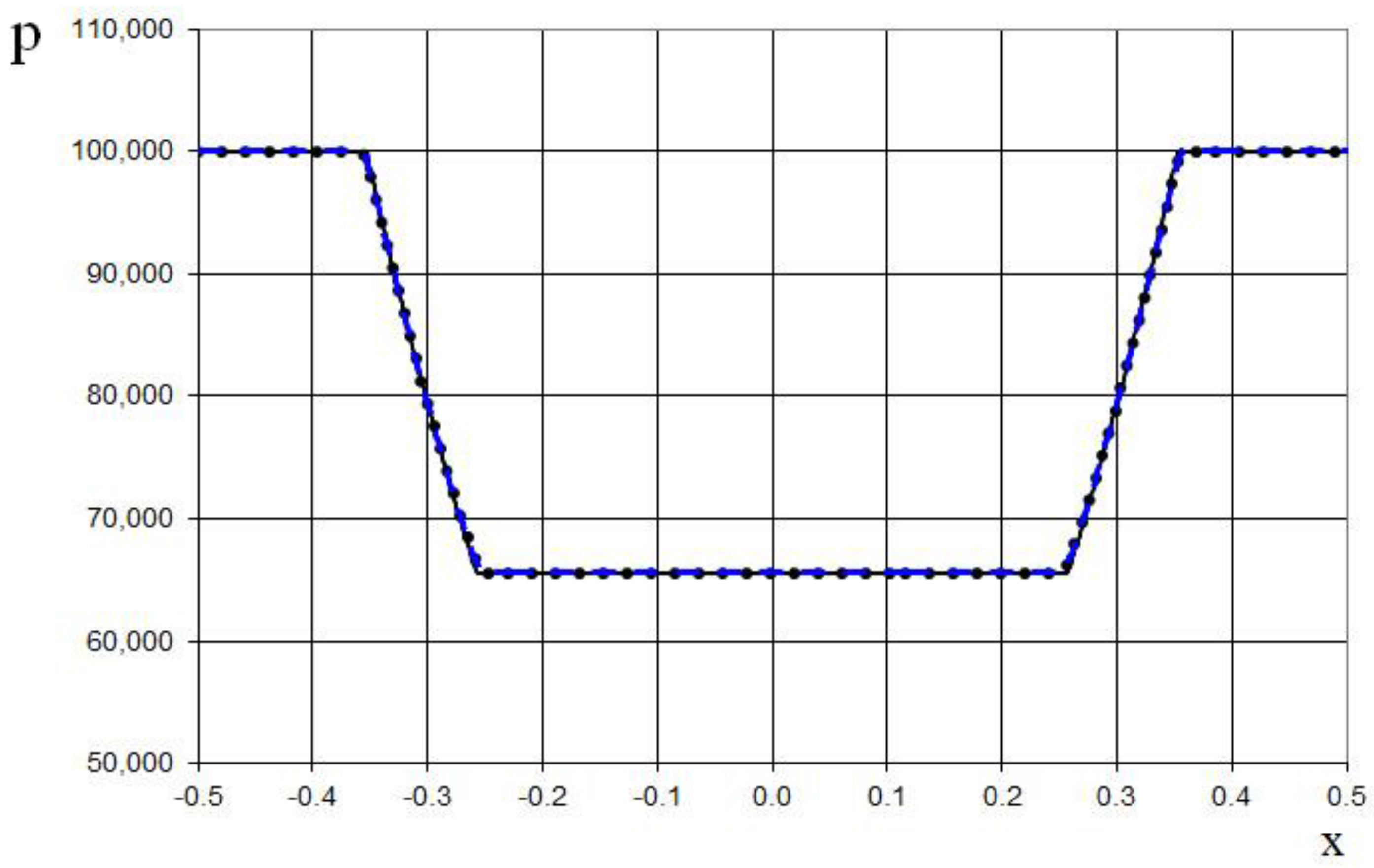
Figure 20.
Density plot for the problem (63): the exact solution (line), the previous method [19] (cross) , and the present method (circle).
Figure 20.
Density plot for the problem (63): the exact solution (line), the previous method [19] (cross) , and the present method (circle).
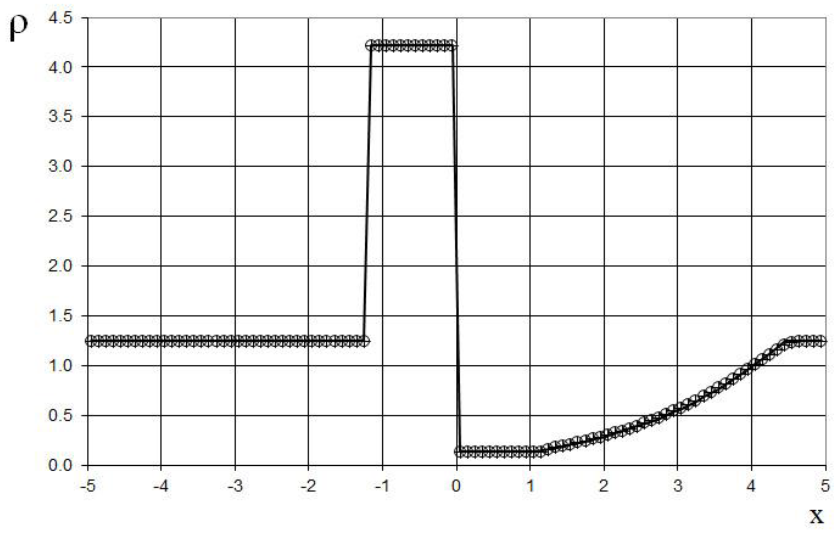
Figure 21.
Velocity plot for the problem (63): the exact solution (line), the previous method [19] (cross) , and the present method (circle).
Figure 21.
Velocity plot for the problem (63): the exact solution (line), the previous method [19] (cross) , and the present method (circle).
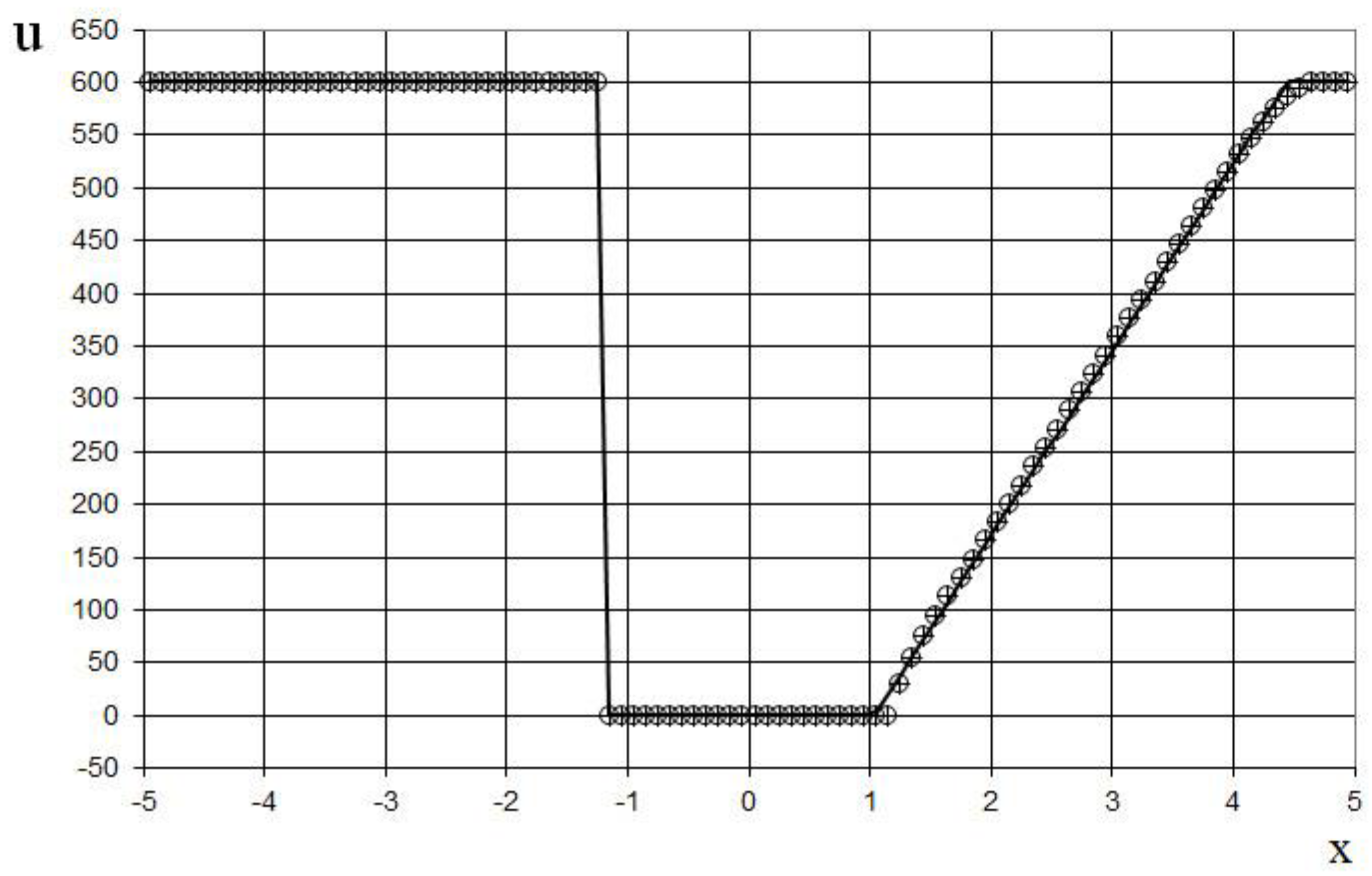
Figure 22.
Pressure plot for the problem (63): the exact solution (line), the previous method [19] (cross) , and the present method (circle).
Figure 22.
Pressure plot for the problem (63): the exact solution (line), the previous method [19] (cross) , and the present method (circle).
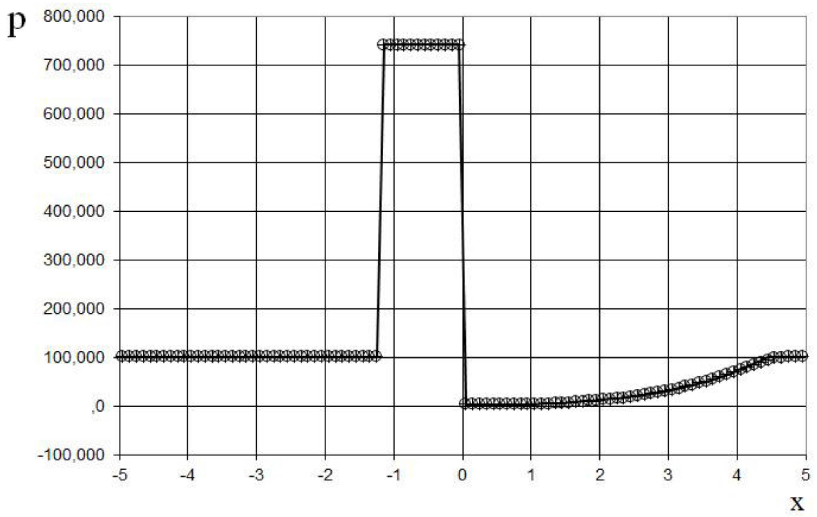
Figure 23.
Density plot for the two Riemann problems interaction (64): the ULT1C scheme of Harten (red dash dotted line), the previous method [19] (black solid line), and the present method (blue dashed line).
Figure 23.
Density plot for the two Riemann problems interaction (64): the ULT1C scheme of Harten (red dash dotted line), the previous method [19] (black solid line), and the present method (blue dashed line).
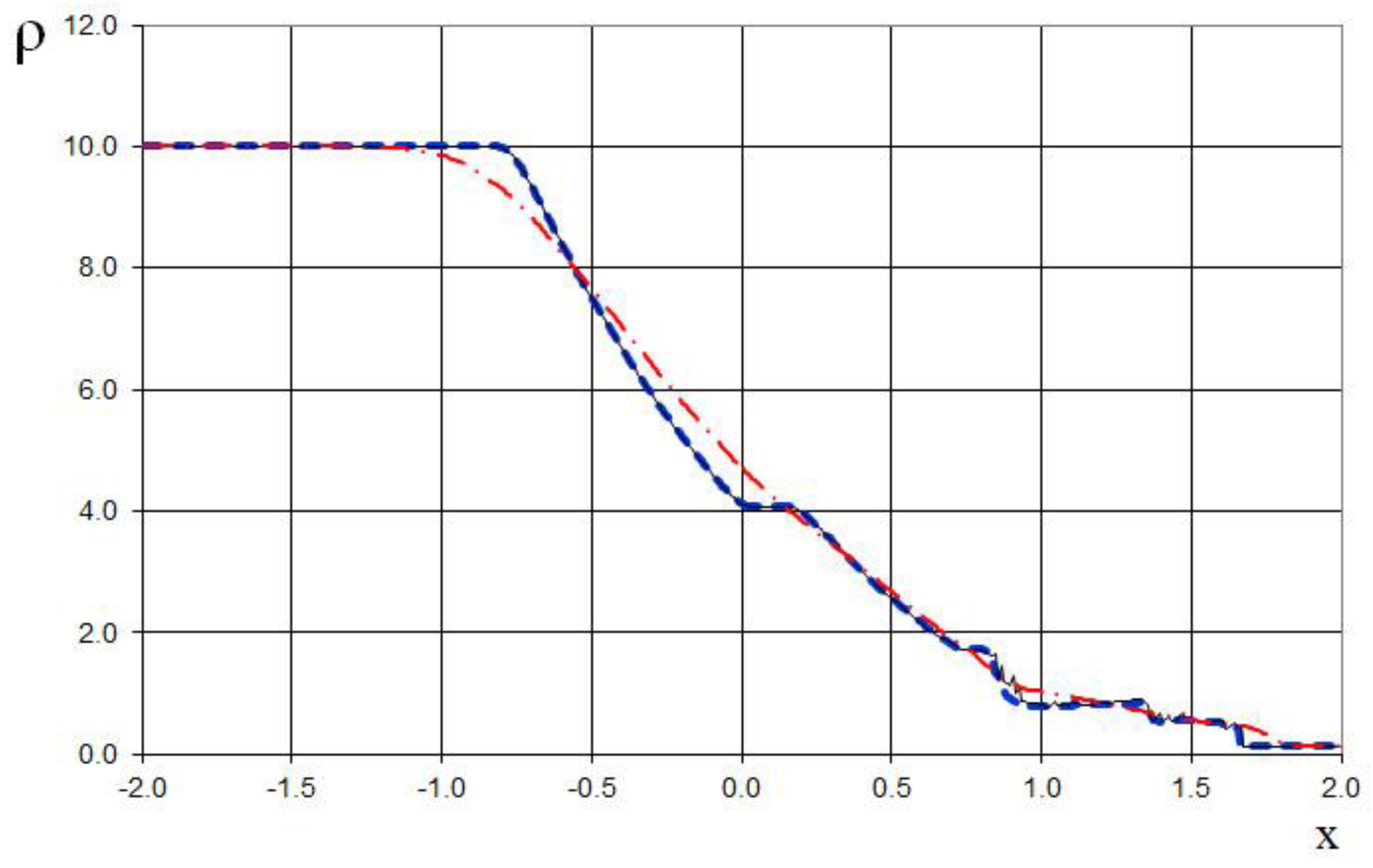
Figure 24.
Magnified view of density plot for the two Riemann problems interaction (64): the ULT1C scheme of Harten (red dash dotted line), the previous method [19] (black solid line), and the present method (blue dashed line).
Figure 24.
Magnified view of density plot for the two Riemann problems interaction (64): the ULT1C scheme of Harten (red dash dotted line), the previous method [19] (black solid line), and the present method (blue dashed line).
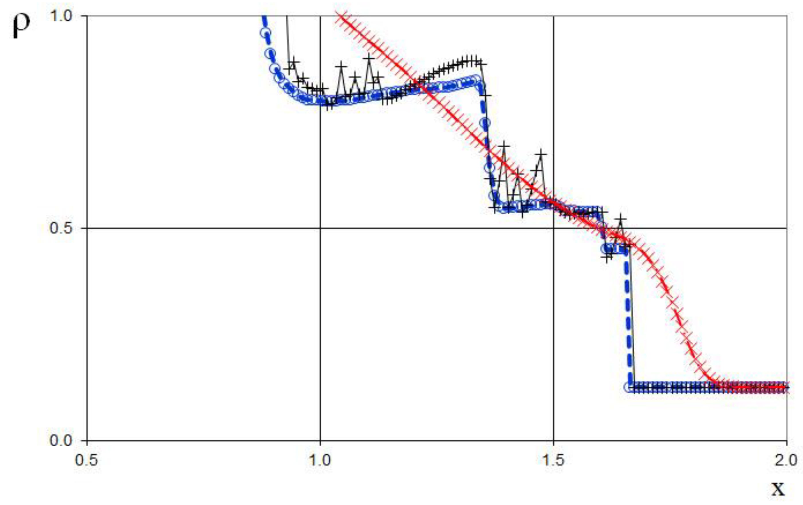
Figure 25.
Velocity plot for the two Riemann problems interaction (64): the ULT1C scheme of Harten (red dash dotted line), the previous method [19] (black solid line), and the present method (blue dashed line).
Figure 25.
Velocity plot for the two Riemann problems interaction (64): the ULT1C scheme of Harten (red dash dotted line), the previous method [19] (black solid line), and the present method (blue dashed line).
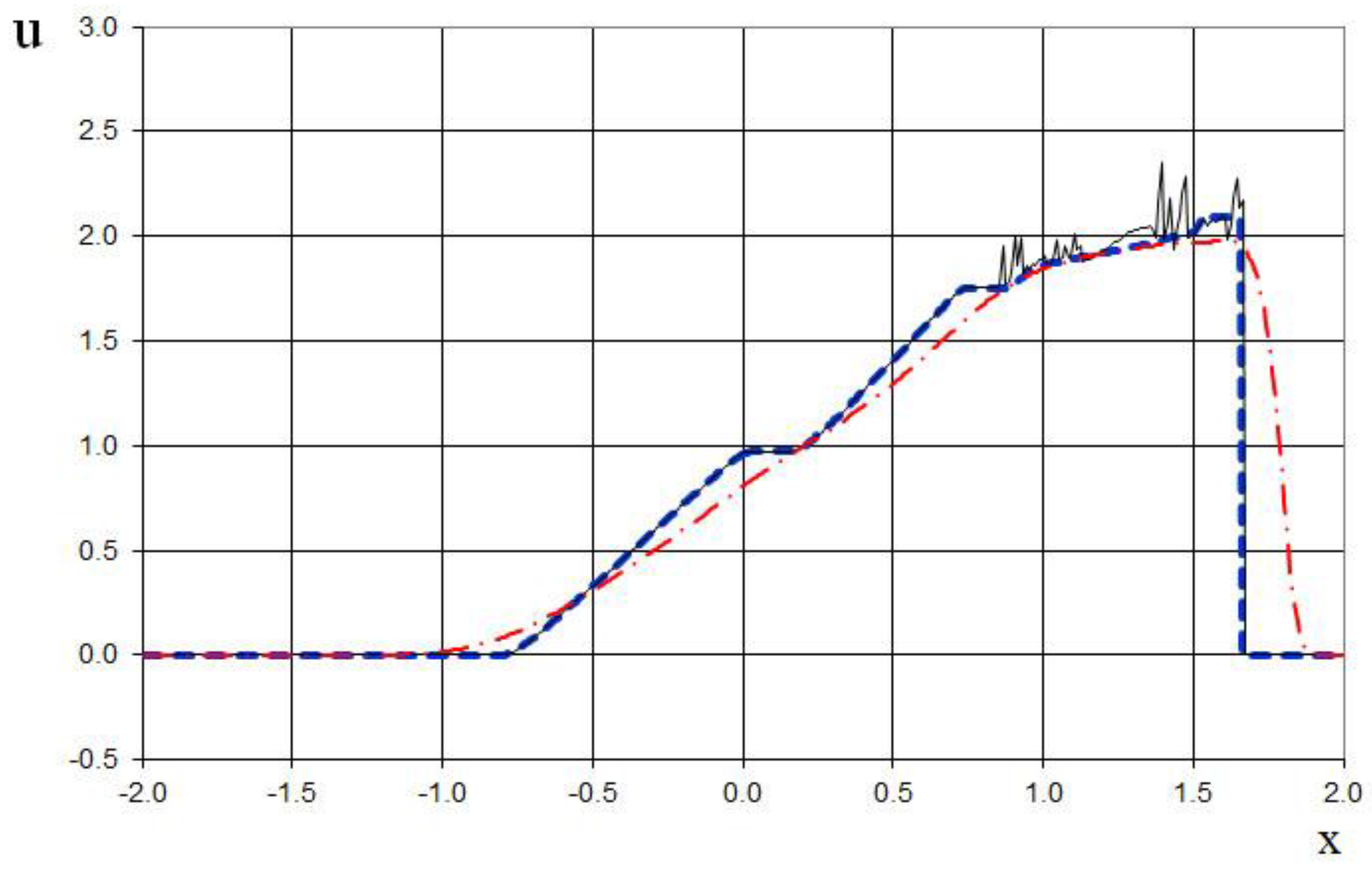
Figure 26.
Magnified view of velocity plot for the two Riemann problems interaction (64): the ULT1C scheme of Harten (red dash dotted line), the previous method [19] (black solid line), and the present method (blue dashed line).
Figure 26.
Magnified view of velocity plot for the two Riemann problems interaction (64): the ULT1C scheme of Harten (red dash dotted line), the previous method [19] (black solid line), and the present method (blue dashed line).
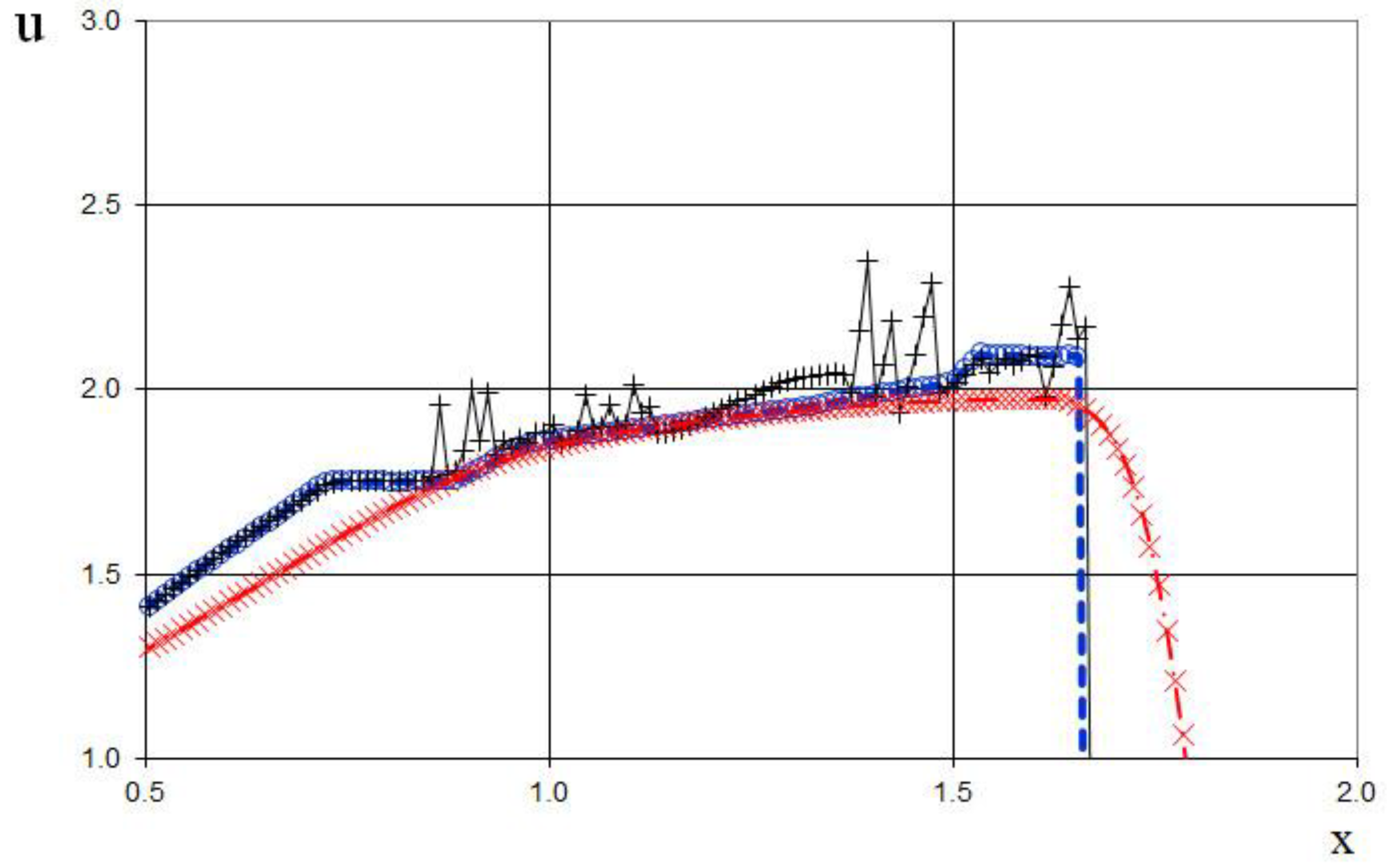
Figure 27.
Pressure plot for the two Riemann problems interaction (64): the ULT1C scheme of Harten (red dash dotted line), the previous method [19] (black solid line), and the present method (blue dashed line).
Figure 27.
Pressure plot for the two Riemann problems interaction (64): the ULT1C scheme of Harten (red dash dotted line), the previous method [19] (black solid line), and the present method (blue dashed line).
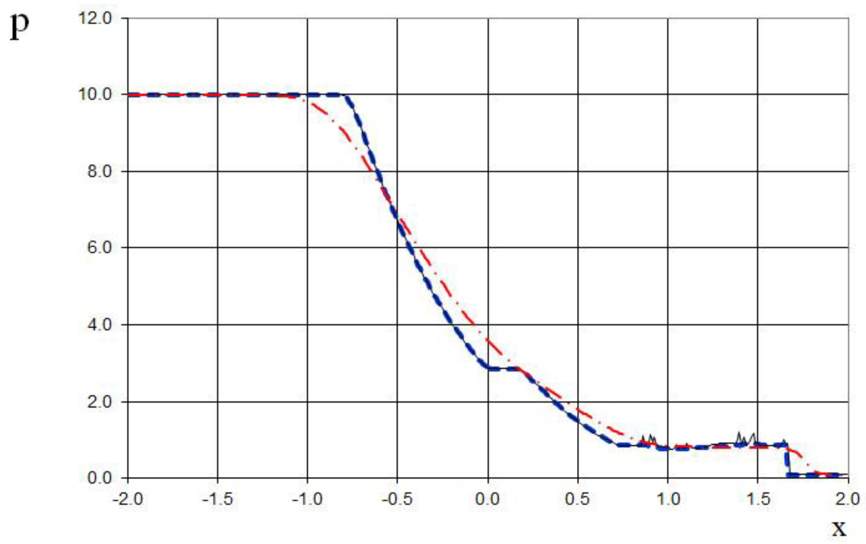
Figure 28.
Magnified view of pressure plot for the two Riemann problems interaction (64): the ULT1C scheme of Harten (red dash dotted line), the previous method [19] (black solid line), and the present method (blue dashed line).
Figure 28.
Magnified view of pressure plot for the two Riemann problems interaction (64): the ULT1C scheme of Harten (red dash dotted line), the previous method [19] (black solid line), and the present method (blue dashed line).
Disclaimer/Publisher’s Note: The statements, opinions and data contained in all publications are solely those of the individual author(s) and contributor(s) and not of MDPI and/or the editor(s). MDPI and/or the editor(s) disclaim responsibility for any injury to people or property resulting from any ideas, methods, instructions or products referred to in the content. |
© 2025 by the authors. Licensee MDPI, Basel, Switzerland. This article is an open access article distributed under the terms and conditions of the Creative Commons Attribution (CC BY) license (http://creativecommons.org/licenses/by/4.0/).
Copyright: This open access article is published under a Creative Commons CC BY 4.0 license, which permit the free download, distribution, and reuse, provided that the author and preprint are cited in any reuse.


